An Optimal Seismic Force Pattern for Uniform Drift Distribution

Abstract

The force distribution proposed by codes, which in many cases is framed in the equivalent static force procedure, likely leads to design structures with non-uniform drift distribution in terms of inter-storey drift and ductility demands. This can lead to an unbalanced drift demand at certain storeys. This phenomenon may also amass cyclic damage to the dissipative elements at this very storey, therefore increasing the probability of premature failure for low-cycle fatigue. This work proposes a new force design distribution that accounts for higher mode effects and limits the displacement concentration at any storey thus improving the dissipative capacity of the whole structures. The main advantage of the proposed method stands in its formulation, which allows to spare any previous set up with structural analyses. The proposed force distribution has been applied to multi-degree-of-freedom systems to check its effectiveness, and the results have been compared with other proposals. In addition, in order to obtain a further validation of the proposed force distribution, the results obtained by using a genetic algorithm have been evaluated and compared. Additionally, the results provided in this work validate the proposed procedure to develop a more efficient lateral load pattern.

1. Introduction

The designer, who designs—or retrofits—a structure which stands in a seismic prone area, must deal with the in-force law for what concerns all the safety checks. Many past seismic events, Northridge (1994), Kobe (1995), Chi-Chi, (1999), L’Aquila (2009), Christchurch (2011) have made apparent that a large number of buildings are still vulnerable to the earthquake effects. Nevertheless, they served as an example and many codes have adjusted their provisions, gaining benefits of feedback. Due to the dynamic nature of earthquakes, codes often provide designers with the equivalent static force approach, which happens to be a realistic estimate of the force that may stroke the structure during its life-cycle. This approach is also advantageous for preliminary design of structures. However, the structures that can be subjected to such a procedure must comply with the definition of regular structure, which mainly refers to mass and stiffness distributions throughout structures. Nevertheless, code provisions give other methods of analysis (e.g., mode superposition procedures, time history procedures) if the criteria of regularity are not fulfilled.

The lateral seismic-force distributions commonly proposed by seismic codes are generally based on a first-mode dynamic solution of lumped multi-degree-of-freedom (MDOF) elastic systems [1,2,3,4,5]. The base shear force $F_b$ for each horizontal direction is determined as a function of the global structural seismic mass M, and of the building location through the pseudo-acceleration design value $S_d$, which corresponds to the fundamental period of vibration $T_1$. According to codes, this base shear has to be distributed proportionally to the storey masses being recognised that first elastic mode shape is mostly predominant. As a consequence, the employment of such a load pattern does not guarantee the optimum use of materials in the nonlinear range of behaviour [6,7,8,9]. However, the common designer is pushed to use such force distributions by static analyses and also when non-linear analyses (e.g., pushover) are performed [10,11].

Non-linear dynamic analyses carried out on seismic resistant structures and also shaking table tests [12,13,14] designed according to a force distribution compliant with the Eurocode 8 (EC8) [5] have often pointed out that top storey structures are subjected to high inter-storey drift demand [15,16,17]. This effect increases as far as the number of storeys increases and was also proved by the findings of Ruiz-Garcia 2010 [18]. Furthermore, this work underlines a larger demand of residual displacements in the upper part of multi-storey buildings if the first-mode proportional force distribution is applied to design them. This could be likely due to higher mode effects [18]. To face this problem, many codes propose different patterns for horizontal force distributions, inter alia, UBC [19], ASCE 7-10 [20] and SEAOC 1999 [21], which are still framed in the equivalent force methods. One other effective force distribution is the one proposed by Chao et al. [1] in which a concentrated force of high magnitude is applied to the very top storey.

The distribution of forces structures are designed with plays a paramount role in the development of a collapse mechanism of global type [22,23,24,25]. In fact, more than in the structures designed according to the so-called hierarchy criteria, in structures designed by way of the kinematic theorem of plastic collapse extended to the second order effects the properly choice of a pattern of forces deeply affects the design outcomes and the structural response. The force distributions is summoned in the computation of virtual external work both in the case of first and second order effects. As a consequence the application of a force with higher magnitude at the top storey tends to redistribute the design moment required at each storey to assure a properly plastic distribution.

In this paper, a new design force distribution is proposed to overcome, on one hand, the limitation of the force distributions that deal merely with the first mode shape and on the other hand the problem of high inter-storey drift demands concentrated at any storey. The mathematical formulation that leads to the definition of the proposed design force distribution is provided and its general validity is underlined. As a matter of fact, the lateral load pattern follows straightforwardly from a linear combination of the excitation vectors—directly related to the mode shapes—which avoids any preliminary numerical analysis. Many simulations on MDOF systems have been performed to confirm the effectiveness of the proposed distribution and then compared with the other ones. Finally, a genetic algorithm is employed to provide a solution with general validity to compare with. The results show that the proposed distribution can slightly outdo the most efficient that can be found in the literature.

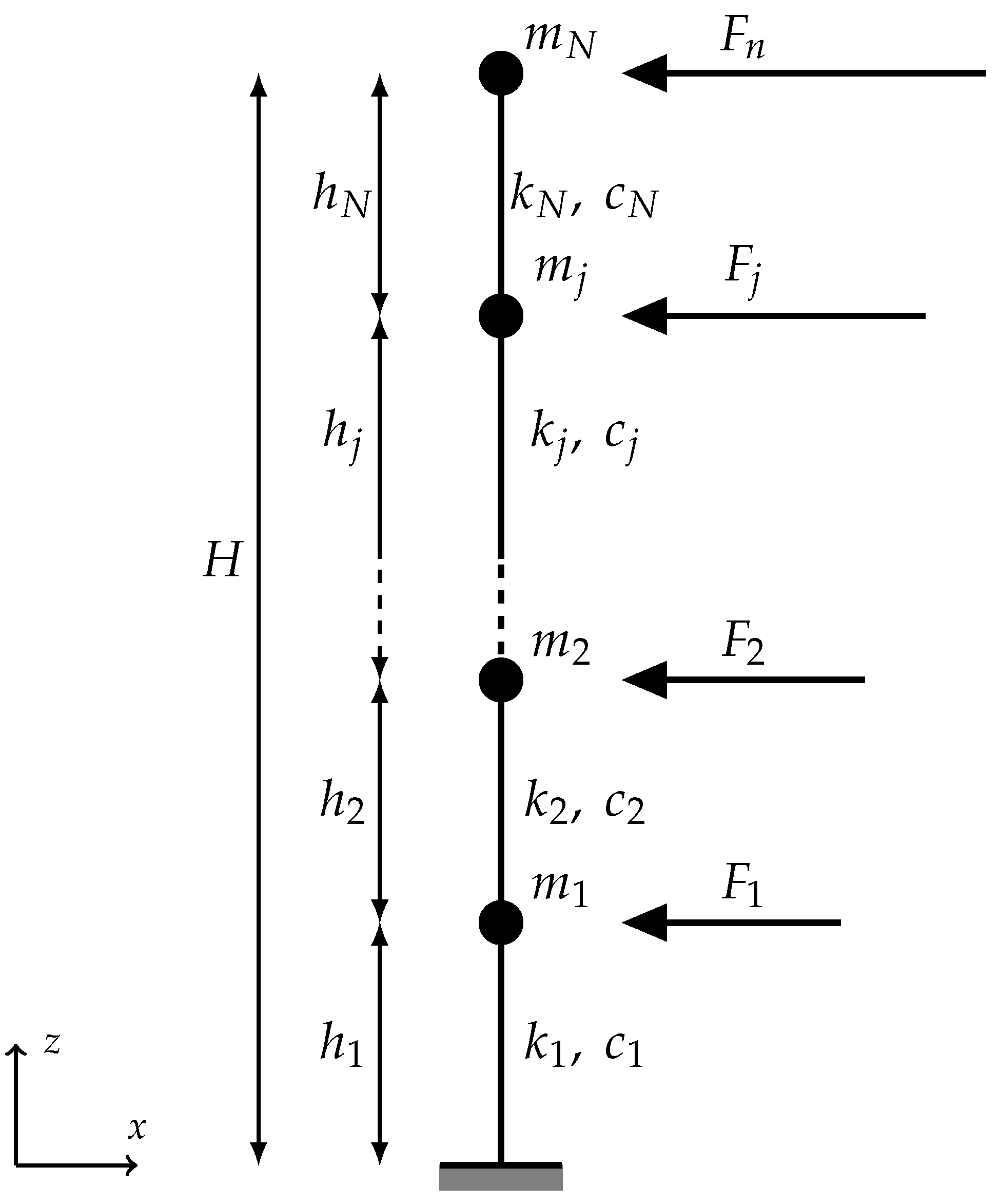
2. Shear-Building Model

The structural model herein considered is a shear-buildings model (SBM). SBM is a model very apt for emulating multi-storey structures which can be also characterised by different dynamic parameters [26]. It represents a model as simple as numerically efficient, which can be employed for time history analysis of multi-degree-of-freedom systems. It can reasonably catch the higher mode effects for the first few effective modes [27,28]. For these reasons, SBM can be suitable employed for studying the load pattern of the seismic actions.

Such a model allows to perform parametric analyses of structures with several degrees of freedom, subjected to dynamic analyses. Figure 1 shows the SBM with N storeys employed for investigating the effects of several height-wise force distributions. Each level of this model is characterised by a lumped mass $m_j$, a spring that connects the level with the one below, whose stiffness is $k_j$, a viscous damping parameter $c_j$ which accounts for mechanical energy dissipation due to the relative motion all over the structural elements. The stiffness $k_j$ at each level is proportioned by the storey shear force coming from the lateral force distribution under study, over the elastic deformation threshold (i.e., ${\delta }_{y.j}$) at each storey. The viscous damping coefficient $c_j$ are not directly tuned, though. Instead, the damping model adopted is the Rayleigh damping model which provides a value of $\xi$ assigned to both the first vibration mode and the ith vibration mode, whose cumulative participation mass is a fixed percentage of the total one.

For the analyses performed within this work the value of $\xi =0.05$ has been assigned to the first two vibration modes; the masses and the inter-storey heights are set to $m_j=m=64$ Mg and $h_j=h=3.00$ m for all the storeys. The value of the ${\delta }_{y.j}={\delta }_y$ is fixed to 0.010 h, even though this value is not used in the numerical model that is employed to solve the linear dynamic analyses. It is worth noting that the way the characteristics of structures have been chosen leads to fulfil the definition of regular structure as introduced in most of the code provisions. However, some of the structures involved in the next analysis may violate some criteria for regularity in elevation, for the non-code compliant load patterns do not take into account such constraints. The responses of the structures are evaluated by means of linear time history analyses performed within the OpenSEES framework [29], which is developed by the Pacific Earthquake Engineering Research Center (PEER).

The design influence of the lateral load patterns investigated in this study is analysed through linear time history dynamic analyses performed on a set of 942 ground motion records registered from 236 seismic events, all of them retrieved from the ground motion database of the Consortium of Organisations for Strong Motion Observation Systems (COSMOS) [30]. Their moment magnitudes range from $5.40$ to $7.20$, whereas the epicentre distances from 4.00 km, the closest, to 83.00 km, the farthest. Figure 2 depicts the mean spectrum of all the selected ground motions (red line) compared with the Eurocode8 spectrum, whose parameters are show the

Table 1. Values of the parameters describing the $Type1$ elastic response spectrum as defined in EC8.

$\mathit{Ground}\mathit{Type}$	S	${\mathit{T}}_{\mathit{B}}\left[\mathit{s}\right]$	${\mathit{T}}_{\mathit{C}}\left[\mathit{s}\right]$	${\mathit{T}}_{\mathit{D}}\left[\mathit{s}\right]$	${\mathit{a}}_{\mathit{g}}\left[\mathit{g}\right]$	$\mathit{\xi }$
B	$1.20$	$0.15$	$0.50$	$2.00$	$0.30$	$0.05$

.

The design procedure of the N-storey structures to be analysed fulfils the static procedure established in EC8, though lateral force distributions from different code provisions are involved in as well. It adopts design response spectra in order to define the global earthquake effects on structures. The spectrum considered is the one whose parameters are exposed in Table 1 and drawn in Figure 2, due to its agreement with the mean spectrum of the set of ground motions. It should be underlined that the total base shear V, which is distributed among the floors by considering the different height-wise distributions, is always evaluated according to EC8 spectrum, which goes:

$$V=S_d\left(T_1\right)m$$

(1)

where $S_d\left(T_1\right)$ is the ordinate of the design spectrum at period $T_1$; m is the total mass of the building; $T_1$ is the fundamental period of vibration of the building computed as:

$$T_1=C_t{H}^{\frac{3}{4}}$$

(2)

where $C_t=0.050$ and H equal to the height of the building.

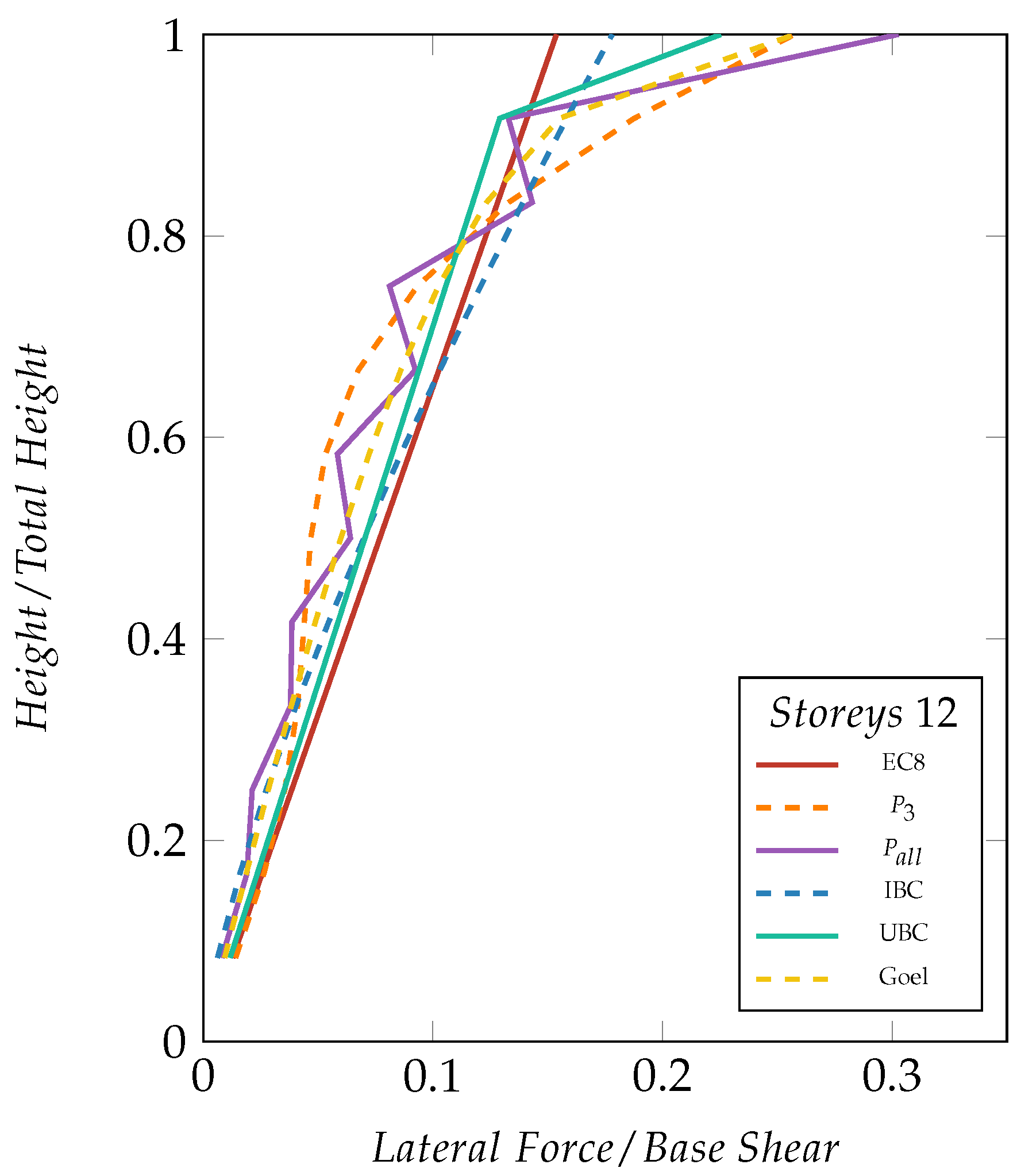
3. Lateral Load Patterns for Seismic Action

3.1. Background

The dynamic equilibrium of the SBM system in Figure 1 can be described by the following system of equations along with some initial conditions [3,31]:

$$\mathit{M}\ddot{\mathit{x}}+\mathit{C}\dot{\mathit{x}}+\mathit{K}\mathit{x}=-\mathit{M}\mathit{\iota }{\ddot{\mathit{u}}}_g$$

(3)

where $\mathit{M}$ is the mass matrix, $\mathit{C}$ is the damping matrix, $\mathit{K}$ is the stiffness matrix, $\mathit{x}$ is the displacements vector, $\mathit{\iota }$ (iota) is the influence vector which represents the displacements of the masses resulting from static application of a unit ground displacement, ${\ddot{\mathit{u}}}_g$ is the acceleration at the base.

In most of the applications, the system of Equation (3) with its boundary conditions can be solved by employing the linear transformation:

$$\mathit{x}\left(t\right)=\mathsf{\Phi }\mathit{q}\left(t\right)$$

(4)

where $\mathsf{\Phi }$ is the modal matrix whose columns are the eigenvectors ${\mathit{\varphi }}_i$, $\mathit{q}\left(t\right)$ is the vector of the displacements in the modal space. The most common way to find the eigenvectors of such a problem is exposed in the following. The free vibrations of a linear undamped MDOF system are described by:

$$\mathit{M}\ddot{\mathit{x}}+\mathit{K}\mathit{x}=\mathbf{0}$$

(5)

Such a system is set into motion from the initial conditions $\mathit{x}\left(0\right)$ and $\dot{\mathit{x}}\left(0\right)$. This circumstances joint with the lack of damping lead to expect the solution of Equation (5) to be periodic:

$$\mathit{x}\left(t\right)=\mathit{\varphi }{e}^{\mathrm{i}\omega t}$$

(6)

where $\mathit{\varphi }$ is an N-dimensional vector of constants, called mode shape, $\omega$ is the frequency of vibration, $\mathrm{i}$ is the imaginary unit. The values of $\omega$ which are solutions of (5) are called the natural frequencies. Either introduction of Equation (6) in (5) and considering the mass matrix $\mathit{M}$ to be non-singular give:

$$(inv\left(\mathit{M}\right)\mathit{K}-{\omega }^2\mathit{I})\mathit{\varphi }{e}^{\mathrm{i}\omega t}=\mathbf{0}$$

(7)

where $\mathit{I}$ is the identity matrix. The solutions of the homogeneous system, as presented in Equation (7), are obtained from the roots of the determinant in the parentheses, where $\omega$ is unknown. In fact, ${\omega }^2$ fulfils the definition of eigenvalue for the matrix $inv\left(\mathit{M}\right)\mathit{K}$. Its positive root identifies the natural frequency and the corresponding eigenvector is the mode shape. As often happens in structural analysis, the matrices $\mathit{M}$ and $\mathit{K}$ are symmetric with real elements, which assure that there exists N real eigenvalues along with their corresponding egenvectors such that the next relationship is satisfied:

$$inv\left(\mathit{M}\right)\mathit{K}{\mathit{\varphi }}_i={\omega }^2{\mathit{\varphi }}_i$$

(8)

This approach is known as modal analysis.

In the modal space, Equation (3) take form as:

$${\ddot{q}}_i+2{\xi }_i{\omega }_i{\dot{q}}_i+{\omega }_i^2{q}_i=-{\ddot{u}}_g{\mathsf{\Gamma }}_{i}i\in [1,\dots ,N]$$

(9)

where ${\xi }_i$ are the damping ratios of the various natural modes, ${\omega }_i$ are the circular angular frequencies, ${\mathsf{\Gamma }}_i$ are the modal participation factors, N is the number of the dynamic degrees of freedom.

At this stage, it is fairly possible to back transform the solution of the uncoupled equations in the Equation (9) in the original spatial coordinate system, that is, solving separately several SDOF systems. It is convenient, however, to consider the response spectrum approach, whose interest is solely focused on the maximum of $q_i$, which is the maximum displacement corresponding to each mode yields to:

$${\mathit{u}}_{i.max}={\mathsf{\Gamma }}_i\frac{T_i^2}{4{\pi }^2}{A}_i(T_i,{\xi }_i){\mathit{\varphi }}_i$$

(10)

where $T_i$ is the period corresponding to the eigenvalue ${\omega }_i$, $A_i$ is the value of the pseudo-acceleration.

Finally, the displacement pattern in Equation (10) can be linearly transformed into the seismic static forces, which are regarded as to the forces that produce the displacements evaluated by means of dynamic analyses [32]. Additionally, once the modal analysis has been carried out, the internal forces are evaluated through the response spectrum analysis:

$${\mathit{f}}_i={\mathsf{\Gamma }}_i{A}_i\mathit{M}{\mathit{\varphi }}_i$$

(11)

Let us now focus on the building structure model herein considered. The mass matrix $\mathit{M}$ turns to be diagonal and the vector $\iota$ equal to $\mathbf{1}$. Such circumstances leads to a special form for Equation (11):

$${\mathit{f}}_{i,j}=\frac{w_j{\mathit{\varphi }}_{i,j}}{{\sum }_j{w}_j{\mathit{\varphi }}_{i,j}}{\mathsf{\Gamma }}_i{L}_i{A}_i$$

(12)

where the $w_j$ represent the mass at the jth storey, the term ${\mathsf{\Gamma }}_i{L}_i{A}_i$, which comes from Equation (11), is the base shear force at the ith mode. Note that the ${\mathsf{\Gamma }}_i{L}_i$ is also called the effective modal mass corresponding to the ith vibration mode. The forces evaluated through (12) simulate exclusively the peak response—displacements and internal forces—of the seismic lateral actions [3].

3.2. Code Compliant Lateral Load Pattern

3.2.1. Eurocode 8—EC8

Eurocode 8: Design of structures for earthquake resistance (EC8) is the reference code of European zone since 2004 by the European Committee for Standardization (CEN). EC8 fully enforces on the lateral force method, as many other code provisions do. The base shear force V, which represent the seismic action effects, has to be distributed along the height of the building. The height-wise shape can be either done by means of the Equation (12) or the following:

$$F_x=\frac{\left(s_x{w}_x\right)}{{\sum }_{j=1}^n{s}_j{w}_j}V$$

(13)

where $s_j$ are the displacements of the masses $w_j$ in the fundamental mode shape. $F_x$ represent the seismic action to be used at each level of the structure.

3.2.2. Uniform Building Code—UBC

The Uniform Building Code, volume 2, “Structural Engineering Design Provisions” issued by the International Conference of Building Officials (ICBO), 1997 edition, often referred to as UBC-97, grounds on equivalent static force approach when regular structures are addressed [33]. The earthquake loads are given for use with load and resistance factor design. The total base shear $(V-F_t)$ is distributed over the height by the formula:

$$F_x=\frac{(V-F_t)\left(w_x{h}_x\right)}{{\sum }_{j=1}^n{w}_j{h}_j}$$

(14)

where, V is the base shear force, $w_j$ and $w_x$ are the weights at a particular level; $h_j$ and $h_x$ are the height of a particular level above the shear base; $F_t$ represents the extra force to be applied at the top level. The magnitude of such a force is computed by $F_t=0.07TV\le 0.25V$, where T is the building period. The UBC-97 states that the $F_t$ takes the greater participation of higher modes into account in the response of longer period structures, i.e., $T>0.70$ s.

3.2.3. International Building Code—IBC

Although 2000 International Building Code (IBC) is extensively similar to UBC-97, and although they are both based on equivalent lateral force procedure for seismic design of buildings, they are fairly different in the seismic provisions [34]. In fact, the vertical distribution of seismic forces of IBC at any x level is a portion of the total base shear:

$$F_x=\frac{w_x{h}_x^k}{{\sum }_{j=1}^n{w}_j{h}_j^k}V$$

(15)

where the parameter $k=0.75+0.5T$, which is limited from below by $1.00$ and from above by $2.00$. For structures with $T<0.50$ s, i.e., $k=1.00$, $\mathit{F}$ shapes a straight line, if masses are evenly distributed over the height. Conversely, for structures with $T>2.50$ s, i.e., $k=2.00$, the forces shape a parabolic distribution with the vertex at the base. The parabolic distribution of the IBC also shifts more forces towards the top. Again, the IBC provisions state for tall regular buildings where the participation of higher modes is significant, the forces have to be shifted towards the top of the building.

3.3. Other Lateral Load Pattern

Goel et al., 2010—Goel

Based on an former proposal by Lee and Goel (2001) [35], and based on the format of the IBC/NEHRP provisions, Goel et al. [36] suggested the following pattern for shear force distribution:

$$F_x\left(T\right)=({\beta }_x-{\beta }_{x+1}){\left(\frac{w_N{h}_N}{{\sum }_{j=1}^N{w}_j{h}_j}\right)}^{\alpha T^{-0.2}}V,{\beta }_x={\left(\frac{{\sum }_{j=x}^N{w}_j{h}_j}{w_N{h}_N}\right)}^{\alpha T^{-0.2}},i\in \left[1,2,\dots n\right]$$

(16)

where $\alpha$ is a parameter set to $0.75$, ${\beta }_{N+1}$ is set equal to 0. However similar to what IBC proposed, the approach proposed by Goel et al. comes from averaging the shear distribution of several non-linear dynamic analyses, which were performed on real structures. The shape of the lateral force distribution takes into account extra information about the structures by means of the fundamental period of vibration. This results in an force-shape quite dissimilar from the first mode shape.

3.4. Proposed Load Pattern—$P^{all}$ & $P^3$

Considering a load case where the lateral forces share the same pattern $p\left(t\right)$, the spatial distribution of the applied forces can be considered to be proportional to a non-time dependent vector $\mathit{s}$ excitation vector [3] as follows:

$$\mathit{s}=\mathit{M}\mathit{\iota }$$

(17)

From the modal expansion of this last vector, the contribution of the ith mode to $\mathit{s}$ can be assessed by:

$${\mathit{s}}_i={\mathsf{\Gamma }}_i\mathit{M}{\mathit{\varphi }}_i$$

(18)

Standing on this, it is possible to define the vector $\widehat{\mathit{b}}$, which is intended as a load pattern, by means of a linear combination of the n ${\mathit{s}}_i$ vectors obtained through the Equation (18) [37]:

$$\widehat{\mathit{b}}=\frac{\alpha {\mathit{s}}_{\mathbf{1}}+\beta {\mathit{s}}_{\mathbf{2}}+\cdots +\psi {\mathit{s}}_{\mathit{n}}}{\left|\right|\alpha {\mathit{s}}_{\mathbf{1}}+\beta {\mathit{s}}_{\mathbf{2}}+\cdots +\psi {\mathit{s}}_{\mathit{n}}\left|\right|}$$

(19)

where $\alpha ,\beta ,\dots ,\psi$ are some scalars chosen in $\mathrm{I}\mathrm{R}$. One can note that the denominator is just for normalisation purpose. The arbitrary of the coefficients in the combination allows for differently weighing the contribution of each mode shape and also to include a different number of mode. Such a circumstances will be exploited to compare the effectiveness of considering the effects of higher modes of vibration.

The scalars that weight each modal contribution to the excitation vector have been set up using the function $f\left(m\right)=-1^m$, where $m\in \mathbb{N}$. This mirrors the properties of sign for the eigenvectors for the $N^{t}h$ element of each vector. Therefore, Equation (19) can be generalised using the following expression:

$$\begin{array}{cc}\hfill F_x=\widehat{\mathit{b}}=& -\frac{\mathit{b}}{\left|\mathit{b}\right|}\hfill \end{array}$$

(20a)

$$\begin{array}{cc}\hfill b_j\left(x\right)=\sum _{i=1}^x{(-1)}^i{s}_{i,j},& x\in \mathbb{N}\cup x\le N\hfill \end{array}$$

(20b)

It is important to stress that the shape of the vector $\mathit{b}$, which can be intended as a lateral load pattern, can be obtained performing a modal analysis. It requires indeed to compute the eigenvalues and the related eigenvectors, which can be accomplished with a programming language. This formulation, which introduces x as a free parameter, makes possible to generate different load patterns on account of how many mode shapes are involved in. For instance, if $x=1$ is introduced in (20b), it gives back the first mode shape vector ${\varphi }_1$. On the other hand, further values of x give back different shapes.

In the following, two proposed lateral force distributions given by Equation (20a) will be studied. The first one, which is called $P^3$, is obtained with $x=3$, that is, the first three vibration modes are accounted for. The latter, which is called $P^{all}$, is obtained with $x=N$ and all the vibration modes are taken into account.

4. Results and Discussion

To compare the 6 above listed load patterns, a 12-storey SBM is designed to be subsequently analysed through time-history analyses. The shear force at each storey, which comes from the aforementioned load patters under study, is turned into stiffness through:

$$k_j=V_j/{\delta }_{y.j}$$

(21)

where $k_j$ is the stiffness to be assigned at the storey spring, $V_j$ is the storey shear force and ${\delta }_{y.j}$ is the yielding threshold. All the N $V_j$ storey shear forces make up the vector $\mathit{V}$, vector of the storey shear forces.

4.1. Adopted Design Procedures

For what concerns the patterns picked out from code provisions ($EC8$, $UBC$, $IBC$), the design procedure is solved in a closed form for codes provide simplified rules to evaluate the fundamental period of structures and, as a consequence, the base shear, i.e., the total horizontal forces, can be evaluated as reported in the Equations (1) and (2). The shapes of the lateral forces induced on structures by seismic events in Equations (13)–(15) are indeed given once the masses and inter-storey heights are defined. Then, by means of Equation (21), the values to be assigned to the elastic springs are computed.

It must be noted that the code provisions methodology for the assessment of the fundamental period of structures relies on an empirical formula, which does allow to attain this preliminary information regardless of structures [38]. However, either the proposed procedure and the one proposed by Goel et al. have been designed considering the actual dynamic characteristics of the structures. To do that, for Goel, $P^3$, $P^{all}$, the formulae must be iterate by the two-steps design-&-modal analysis procedure. The design of the SBM systems is hence done by an iterative procedure for $P^3$, $P^{all}$ and Goel because the period of vibration has been evaluated on the designed structure. Algorithms 1 and 2 show the pseudocodes of the numerical procedures that have been coded to design the structures with the non-code compliant lateral load pattern.

Once the input parameters are defined (i.e., number of storeys N, mass m, inter-storey height h, the base shear force V and the plastic threshold ${\delta }_y$), the procedure Algorithm 1 starts with a tentative period of vibration $T_1$. Its definition comes from the proposal of $EC8$ (Equation (2)), which, however little differences, is quite common among codes. It should be noted that whatever the initial value the procedure is stable and leads to the same result. Afterwards, once the lateral force distribution $\mathit{F}$ has been computed, the values of the $k_j$ are estimated through Equation (21) and hence the structure is assigned. Therefore, the structure undergoes modal analysis to obtain its actual periods of vibration. At this point, the loop ends and the procedure goes back to the definition of a new value of $\mathit{F}$, whose input parameter is updated to the actual one.

Although Algorithm 2 may appear different, it traces the same essential steps of the previous one. It is worth noticing that this procedure requires an extra input parameter, which is used to consider a different number of mode shapes for computing the lateral force distribution. The variable $N_{modes}$ indeed refers to the number of mode shapes to be included in Equation (20b). In this work, the value $N_{modes}=3$ is used to generate $P^3$ whereas $N_{modes}=N$ for $P^{all}$. Prior to define the structure, a tentative lateral force distribution $\mathit{F}$ is assumed, which allows for designing and performing the modal analysis. It is now possible to compute the lateral force distribution, which therefore makes feasible the evaluation of the exit statement. Unless the exit statement is fulfilled, the procedure goes on seeking for convergence.

It is essential to point out that the procedures, which were coded in Matlab scripts [39], deliver the matrices of stiffness K in a few loops. The eigen values are evaluated by solving Equation (8) considering the diagonal matrix $\mathit{M}$, whose generic elements are $m_{j,j}=m$. The stiffness matrix $\mathit{K}$ is built considering that the diagonal elements are $k_{j,j}=k_j+k_{j+1}$ and the off-diagonal elements are $-k_{j-1,j}=-k_{j,j-1}=k_j$ with $j\in [1,N]$. It should be noted that when j is out of its range, the element is assumed to be 0. The assessment of eigenvalues and related eigenvectors is performed by means of the Cholesky factorization, which exploits the $LU$ decomposition. If applied to tri-diagonal matrices, and such is the instance, the decomposition is very efficient as the computational cost reduces to $O\left(N\right)$ flops.

Algorithm 1: Pseudocode for Goel design-procedure.

Algorithm 2: Pseudocode for $P^3$ and $P^{all}$ design-procedures.

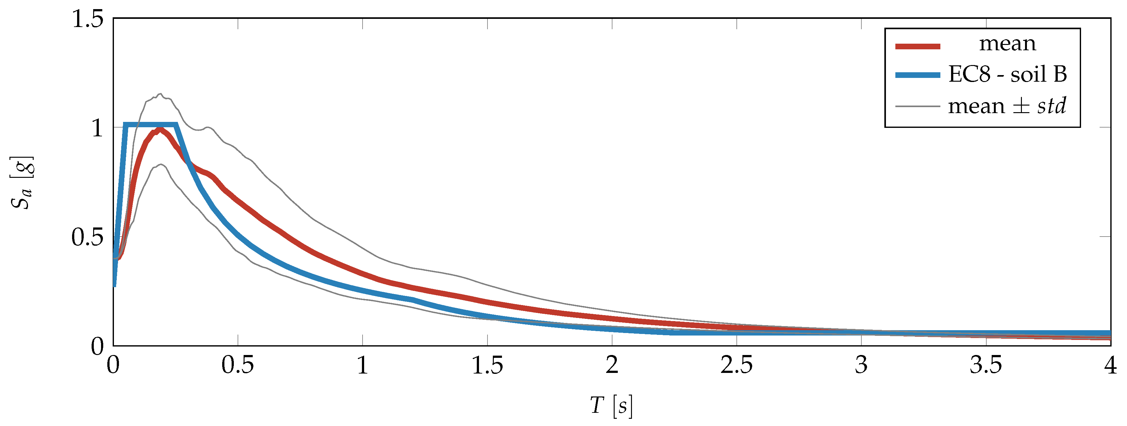
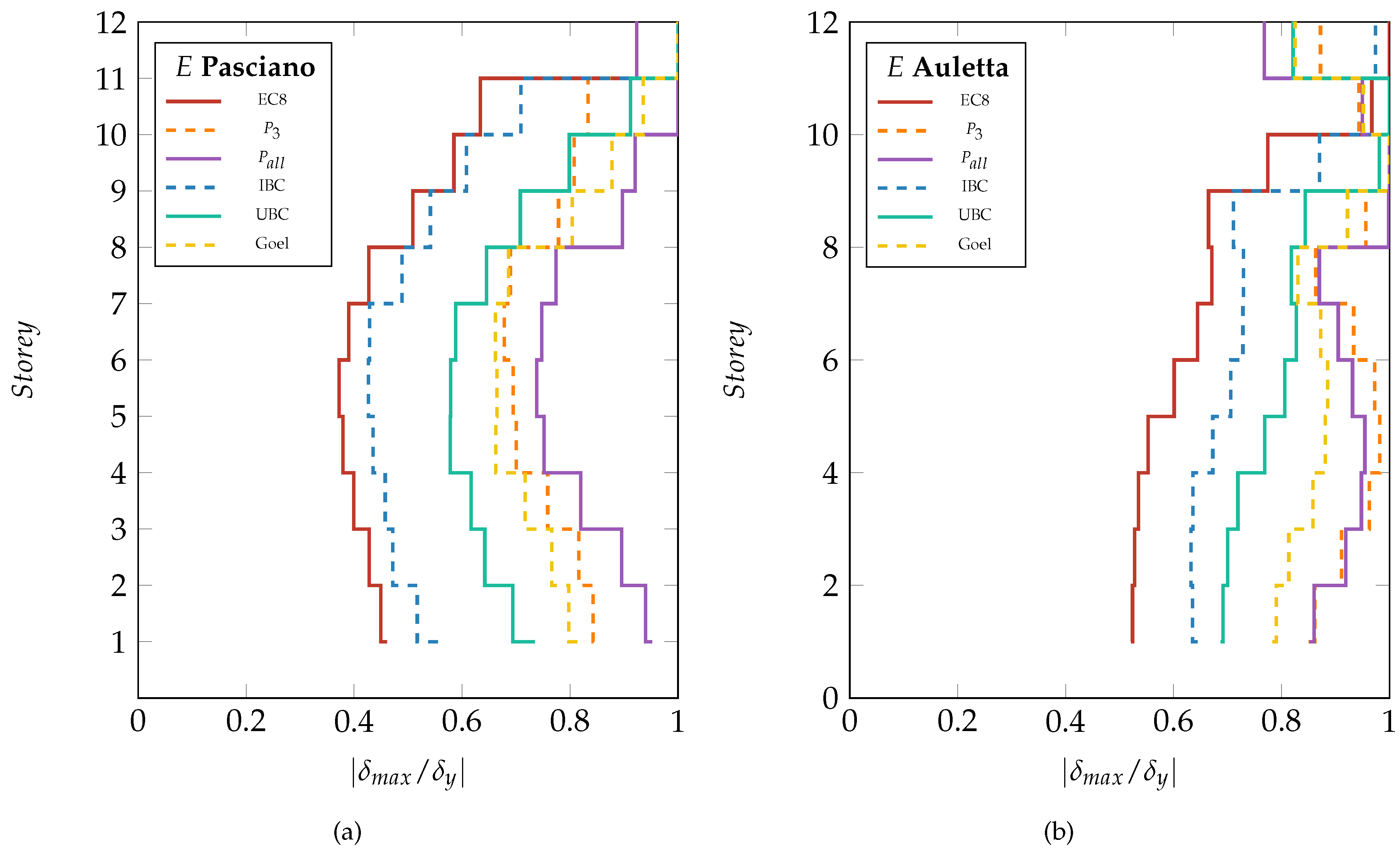
4.2. Effect of Earthquake Excitation and Comparison

Figure 3 depicts the shape of the lateral patterns employed for the seismic design of the 12-storey SBM, whose masses and inter-storey heights are constant all over the levels, as specified before. All the distributions prescribe force increasing with the height. $IBC$ (blue dashed line), which shapes forces according to a super-linear curve, shifts little force to the upper levels of the structure. The remaining distributions are characterised by a conspicuous shift of force to the upper storeys. This circumstances may be explained by a hunch about the floor accelerations, which tend to increase along with the height of the structure. Meanwhile $UBC$ (green solid line) and $IBC$ definitely state that a shift of force to the upper levels is due to higher mode effects are taken into account, the shape of Goel (orange dashed line) comes directly from observation of the shear pattern induced by ground motions on real structures. Eventually, the proposed load patterns $P^3$ and $P^{all}$ can naturally account for more vibration mode effects for their shapes come from superposition of the effect of many mode shapes.

Therefore, the 6 load patterns under study were used to design 6 structures, respectively. The structures were set up following the procedures exposed in Section 4.1 and subjected to two different earthquake ground motions. The results of such analyses are hence gathered into the vector ${\mathit{\delta }}_{max}$, whose element are the maximum inter-storey drift at each level ($|{\delta }_{max,j}|$) occurred during the dynamic analysis of the structure. The multipliers that modify the amplitude of the two ground motions are set such that to lead structures to exhibit a maximum displacement equal to ${\delta }_y$. Note that the two earthquakes used for Figure 4 were randomly singled out from the ground motion ensemble to show the dependence of the structural response on the earthquake variability.

Figure 4a,b report on the x-axis the maximum dimensionless relative displacement at each level $|{\delta }_{max,j}/{\delta }_y|$ corresponding to each storey. Each curve reported in the two panels depicts the data related to a different load pattern, as reported in the legends, used for design purposes. Figure 4a,b refer to the SOUTHERN ITALY 1980—Pasciano cimitero—HNN and the CENTRAL ITALY 2016—Auletta (Petina)—HNN strong motions, respectively. Figure 4 shows that the structures, which have been designed with load patterns prescribing larger forces at the topmost storey, give better results in term of maximum relative displacement distribution. The distribution $IBC$, which is slightly different from $EC8$, outdoes the first-mode-proportional pattern, even if it additionally accounts for the second mode. These first two also share another flaw which is the fact that the maximum relative displacement is always attained at the last floor. Regarding the $UBC$ code provision, it gives reasonable results in term of dispersion around the mean, and it tends to move down the position where the structure attains the maximum displacement. Lastly, the $P^3$, $P^{all}$ and Goel distributions give the best results, providing the hard proof to substantiate the need of considering higher mode effects. Obviously, for lateral resisting structures where the dissipative devices are all over evenly located, the optimum deflected shape would be having all dimensionless relative displacements equal to 1 with a consequent 0-dispersion. As it can be observed from the two panels, the response of the system is strongly dependent on the characteristics of the earthquake records.

The same 6 structures, whose results are reported in Figure 4, have been undergone the whole set of accelerograms (ref. Section 2). Figure 5 collects the results of the linear dynamic analyses averaged over the 942 ground motions. Figure 5a, which reports the mean of the maximum dimensionless relative displacement $|{\overline{\delta }}_{max}/{\delta }_y|$, which is the average of all the $|{\delta }_{max}|$, against the relative height, shows substantial agreement with what is reported in Figure 4. EC8 ans IBC perform the worst, highlighting the crisis, which is related to displacements, at the very top storey in 933 out of 942 simulations. As for the remaining lateral force distributions, the aggregated results draw the same fashion of the previous ones. However, the average process narrows the gap amongst them, proving that they behave almost equally. That is more apparent from the value of the coefficient of variation ($CoV$) of each line reported in the legend.

Additionally, panel Figure 5b shows the cumulative distribution function (CDF) for the random variable G, whose elements g are defined for each deflected shape by means of:

$$g=\frac{1}{N}\sum _{j=1}^N{\left({\overline{\delta }}_j-\overline{\mu }\right)}^2$$

(22)

where $\overline{\delta }$ is the dimensionless deflected shape corresponding to each linear dynamic analysis, $\overline{\mu }$ is the dimensionless average value of the deflected shape. The vector $\overline{\delta }$ is built considering the maximum relative displacement at each storey, then the value of g elements is evaluated through the Equation (22). So that the vector $\mathit{G}$ is a vector that collects all the terms belonging to the analysis of each ground motion and it is composed of 942 elements, one per each ground motion. The results depicted in panel Figure 5b make even clearer the performance exhibited by the structures designed according to the 6 load patterns under study. Again, the worst are EC8 ans IBC whereas the others confirm their aptitude for taking into account dynamic properties of structures.

Figure 6 shows the results of the same analysis performed in the previous paragraph bur the number of storeys. Structures with 9, 15 and 20 storeys were designed with the 6 lateral load patterns under study and hence analysed in the same fashion of the 12-storey structure. The displacement demands are pretty much the same that have been seen before. The $UBC$, $P^3$, $P^{all}$ and Goel keep giving good results, proving that they are able to catch the effects of higher modes. The $CoVs$ depicted in the legend for each curve help make out the differences. For instance, the $CoV$ for $P^3$ and Goel rises from about 0.15 for the nine-storey structure to 0.17 for the 20-storey structure, which means that the displacement demand is quite constant while increasing the height of the structure.

5. Optimum Load Pattern for Seismic Action

Within the elastic range, to determine the optimum load pattern for seismic actions on an SBM, the reference solution of the problem is found by means of an iterative procedure. It should be pointed out that the solution of the problem is represented by a desirable pattern of relative inter-storey drift, that can be changed at will. In this case the reference solution is represented by a pattern of relative displacement characterised by a constant value ${\overline{\delta }}_j$, i.e., the same relative displacements for all storeys. This optimisation problem is addressed by means of heuristic optimisation techniques [40,41,42,43], which are based on the common analysis&redesign procedure [44]. Amongst the members of such a class of algorithms, the genetic algorithm (GA) has been chosen for the aim of this work.

5.1. Genetic Algorithms (GA)

Genetic algorithms were firstly developed by Holland [45] and then extended by Goldberg [46]. GAs are random-based population-based meta-heuristic algorithms, mostly known as a model of the natural selection process that is observed in nature. This method is entrusted to solve difficult optimisation problems, which is already known the answer to. The GA has been chosen because of its ability to work with small populations. Additionally, it almost does not need of any knowledge about the initial state of the system.

The algorithm begins with pseudo-randomly seeding the initial population ${\mathit{P}}^0$ over the search space, whose size is about 100. Each member of the population, i.e., an individual $\mathit{p}$, represents the pattern of the lateral forces, which is characterised by a chromosome length, that is, the number of storeys.

Secondly, the fitness of each individual is evaluated by means of the fitness function, which is defined as follow (step 1 in Algorithm 3):

$$f(\mathit{p},E,\rho )=\frac{1}{\mu }\sqrt{\frac{1}{N-1}\sum _{j=1}^N{({\overline{\delta }}_j-{\delta }_j(\mathit{p},E,\rho ))}^2}$$

(23)

where $\mu$ is the mean of the vector $\mathit{\delta }$, N is the number of storeys, $\overline{\mathit{\delta }}$ is target vector of relative displacements, $\mathit{\delta }(\mathit{p},E,\rho )$ is the vector that collects the maximum relative displacement at each storey of the structure, which depends on the lateral force distribution $\mathit{p}$, the ground motion E, and the scale factor $\rho$ that modifies the amplitude of the ground motion. As for the value of $\rho$, it is evaluated for each simulation such that the value of $max\left(\mathit{\delta }\right)$ is equal to a fixed value ${\delta }_{max}$. As for the target vector $\overline{\mathit{\delta }}$, this represents the target distribution of the maximum relative displacements which, for this work, corresponds to relative inter-storey displacement uniformly distributed, or rather mean of $\mathit{\delta }$ equal to ${\delta }_{max}$ and nought standard deviation.

Thirdly, based on how good each individual fits the exact solution, the population is rearranged in such way the most apt individuals to give good fitness are likely to being duplicated (step 2 in Algorithm 3). The algorithm involved in this phase is the tournament which randomly mixed up the best chromosomes to be recombined. In fact, during crossover, bit of the best chromosomes are selected and mixed up (step 3 in Algorithm 3). The technique involved in this step is the one-step, which randomly fix one pivot in each array corresponding to the winner chromosomes.

Lastly, prior to applying the fitting test to the new population, the mutation is applied to it (step 4 in Algorithm 3). It is managed by a boolean operator which randomly alters the population to explore genetic diversity from one generation to the next. The probability of mutation is tuned by means of a threshold value, which defines the mutation rate for each element of the population. As a safeguard measure, the best individual of the population is always preserved from one generation to the next. The exit statement is fulfilled when the fitness of an individual is less than a certain tolerance ($tol$ in Algorithm 3), delivering the solution to the optimisation problem (step 5 in Algorithm 3).

Algorithm 3: Pseudocode for GA.

5.2. Results

The algorithm herein proposed has been applied to the a 12-storey SBM structure, whose parameters are exposed in Section 2. The GA has been set to find the lateral load pattern whose maximum relative displacements best fits the vector $\overline{\mathit{\delta }}$, which is characterised by all the elements equal to ${\overline{\delta }}_j={\delta }_y$. In other word, the relative deflected shape of the structure under ground motion excitation is a straight line, according to the theory of uniform deformation theory. The population of the GA indeed represents the lateral force distributions to be used for design purpose. In fact, each individual of the population corresponds to a different structure, which is designed with the same procedure exposed in Section 4 and briefly collected in the steps 1.1–1.4 in Algorithm 3. Therefore, the structures are subjected to linear dynamic analyses by means of self-developed code, which was firstly validated against OpenSEES’s solutions [29].

The GA algorithm has been coded in a Matlab program [39]. The code has been mainly written according to what Rice and Nyman [47] suggest in their work. The goodness of each individual is evaluated by means of the fitness function defined as Equation (23). It must be noted that the way the fitness function is defined allows to consider it as the coefficient of variation of that very vector, which represents the lateral force distribution. Therefore, the error that characterises the output of the GA can be tuned by means of the value $tol$, which is set to $4\%$. In order to reduce the run-time of the procedure, the loops of the program were parallelised and run on a multi-core Xeon CPU. Actually, this procedure has been repeated for each ground motion in the whole set of records (942) employed for the assessment of the performance of the 6 investigated lateral force distributions. The procedure proved to converge to the solution after about 150 iterations for most of the ground motions, with a maximum of 8 cycles without any reduction in the value of the fitness function. This was mainly accomplished by imposing as an initial population the lateral force distribution $P^{all}$, which was found to be more appropriate as a solution of this problem from the analyses performed in the previous section. It must be mentioned that 13 procedures out of the 942 considered could not reach the exit threshold (4%). Those simulations were hence stopped after 50 cycles without any improvement, providing an average $CoV$ around 10%.

The results provided by the GA have been collected into the 2 panels in Figure 7. Figure 7a depicts the dimensionless maximum relative displacement $|{\overline{\delta }}_{max}/{\delta }_y|$ distributions of the solutions provided by the GA (thin grey lines) for all the ground motions. Moreover, the mean value of the whole data-set is depicted (red line), which is quite close to the target vector $\overline{\mathit{\delta }}$ (black dashed line). Figure 7b depicts the lateral load patterns provided by the GA (thin grey lines), each corresponding to a different strong motion. All these curves share an higher force to the last two storeys whereas downward the lateral forces can have some negative values. That is not to worry about at all. The dynamic characteristics of each earthquake make the procedure explore and recognise this changing (dropping) in stiffness of the structure useful in equalising the relative displacement demand. However, as is shown by the mean line (red line) that is not the main trend for the lateral forces, even if the first floors of the structures are engaged by forces whose magnitude is low.

It is worth comparing the solution provided by the GA with the load patterns involved in the analyses carried out for this work. Figure 8a,b compare the seismic design load patterns of $EC8$, $UBC$, $P^{all}$, Goel and the corresponding normalised stiffness patterns, respectively, with the range that comes from the GA analysis (dashed red lines). The $EC8$ proposal do not fit the findings of the GA and indeed displays an evident disagreement on the magnitude of the force to be applied at the last floor. This deed could alone explain the bad performance of the $EC8$ load patterns. Conversely, the $UBC$, $P^{all}$, and Goel proposals are inside the range, however differently. The force at the topmost level of the $UBC$ proposal shows a good agreement with the mean value of the GA load pattern whereas the forces to be applied to the other storeys almost trace the $EC8$’s. Additionally, $UBC$ proposal strictly follows the lower bound of the GA solution in term of stiffness pattern. Such a circumstances points explicitly out that the extra force at the top storey is of vital importance for structures under dynamic seismic load if a evenly distributed inter-storey drift is sought. $P^{all}$, and Goel dimensionless stiffness patterns are still close one each other and inside the GA’s range proposed as a reference solution.

6. Conclusions

A massive numerical investigation was carried out to evaluate the ability to provide equal inter-storey drifts of several seismic design load patterns, either selected from code provisions and literature proposals. Additionally, a criteria for deriving a load pattern for uniform inter-storey drift distribution, which inherently accounts for higher mode contributions, was proposed. The performance of the two load patterns, which were built with the proposed procedure, were compared with the other lateral patterns collected from code provisions and the literature. It was demonstrated that the proposed method can produce a lateral load distribution as good as the ones proposed in the literature, irrespective of the height of the building.

The proposed formulation has a more general field of application if compared with the one proposed by Goel et al. [36]. In fact, this lateral force distribution was set up by performing a series of analyses on steel moment resisting frames (MRFs), eccentrically braced frames (EBFs) and concentrically braced frames and using 20 ground motions. Obviously, if the set of considered ground motion changes, the result could change. Similarly, if the structure is different from the one considered in the analyses, the validity of the distribution proposed by Goel et al. cannot be assured. On the contrary, the lateral force distribution herein proposed can be extended to a number of structural schemes and do not rely on preliminary tune-procedures which make the load pattern apt only for that specific case.

The results of linear dynamic analyses performed on structures designed according to 6 different load patterns prove that higher mode effects must be taken into account someway. The $EC8$ and $IBC$ proposals demonstrate to be blind to this and indeed they perform poorly, amassing all the displacement demand in the uppermost storey. The $UBC$ proposal, as simple as it is, gives satisfactory performance close to the lateral force distributions which consider more accurate approaches. As a matter of fact, the force distributions Goel, $P^3$, $P^{all}$ prove the need of stiffen the upper storeys of structures to assure a proper distribution of displacement. Moreover, the extension of the analyses to structures with a different number of storeys showed that the seismic design load patterns $UBC$, Goel, $P^3$, $P^{all}$ have a steady behaviour as well. In fact, the $CoVs$ of the average results are slightly sensitive to the height of structures.

In order to verify the insight gained from the statistics on the linear dynamic analyses results, the optimum load pattern for each ground motion was find by means of a genetic algorithm. The load patterns obtained from it were treated as a reference solution of the problem under study and the results provided by such a procedure confirmed the results obtained by applying the considered load patterns. It can be concluded that there is a need of an extra force to be applied to the uppermost storey of structures, which is crystal clear if the $EC8$ and $UBC$ are alone inspected. In fact, the only remarkable difference is definitely the extra force at the topmost level, which makes the latter load patterns fit the range found by means of the genetic algorithm.

The results provided along this paper and related to the performance of either the proposed procedure and the proposal of Goel et al. make evident that the two patterns are both efficient options. However, it is important to underline their different genesis, albeit a common aim. The two lateral load patterns attempt to equalise the inter-storey drift of structures, according to the theory of uniform deformation. In addition, the procedure proposed by Goel et al. has been successfully extended to steel structures in order to guarantee also an uniform ductility demand. Presently, the proposed procedure has been investigated considering the shear building model which additionally fulfils all the criteria for regular structures. This was employed as to ensure the viability of the code provisions and hence make a fair comparison among all the lateral load patterns considered. Eventually, the procedure proposed in this work needs to meet validation proof against more sophisticated and detailed model of structures. The procedure does not allow for a simplified form however. In the development of this research activity, further studies should be carried out in the future in order to validate the proposed approach. In particular, nonlinear time history analyses will be carried out using accelerograms with spectral content adjusted to the response spectrum adopted for the design procedure. Additionally, the proposed procedure will be applied to more accurate models of structures, e.g., moment resisting frames, concentrically braced frames.

References

1. Chao, S.-H.; Goel, S.C.; Lee, S.-S. A Seismic Design Lateral Force Distribution Based on Inelastic State of Structures. Earthq. Spectra 2007, 23, 547–569. [Google Scholar] [CrossRef] [Green Version]
2. Applied Technology Council. Tentative Provisions for the Development of Seismic Regulations for Buildings; Report ATC 3-06, NBS Special Publication 510, NSF Publication 78-08; National Science Foundation: Washington, DC, USA, 1978.
3. Chopra, A.K. Dynamics of Structures—Theory and Applications to Earthquake Engineering, 4th ed.; Prentice Hall: Englewood Cliffs, NJ, USA, 2012. [Google Scholar]
4. Clough, R.W.; Penzien, J. Dynamics of Structures, 2nd ed.; McGraw-Hill, Inc.: New York, NY, USA, 1993. [Google Scholar]
5. Eurocode 8. EN 1998-1: Design of Structures for Earthquake Resistance—Part 1: General Rules, Seismic Actions and Rules for Buildings; British Standards Institution: London, UK, 2004. [Google Scholar]
6. Ganjavi, B.; Hajirasouliha, I.; Bolourchi, A. Optimum Lateral Load Distribution for Seismic Design of Nonlinear Shear-Buildings Considering Soil-Structure Interaction. Soil Dyn. Earthq. Eng. 2016, 88, 356–368. [Google Scholar] [CrossRef]
7. Jallad, J.; Mekhilef, S.; Mokhlis, H.; Laghari, J.; Badran, O. Application of Hybrid Meta-Heuristic Techniques for Optimal Load Shedding Planning and Operation in an Islanded Distribution Network Integrated with Distributed Generation. Energies 2018, 11, 1134. [Google Scholar] [CrossRef]
8. Palacios-Quiñonero, F.; Rubió-Massegú, J.; Rossell, J.M.; Rodellar, J. Design of Distributed Multi-Actuator Systems with Incomplete State Information for Vibration Control of Large Structures. Designs 2018, 2, 6. [Google Scholar] [CrossRef]
9. Hajirasouliha, I.; Moghaddam, H. New Lateral Force Distribution for Seismic Design of Structures. J. Struct. Eng. 2009, 135, 906–915. [Google Scholar] [CrossRef]
10. Faggiano, B.; Formisano, A.; Castaldo, C.; Fiorino, L.; Macillo, V.; Mazzolani, F.M. Appraisal of Seismic Design Criteria for Concentric Bracing Steel Structures According to Italian and European Codes. Ing. Sismica 2016, 13, 42–50. [Google Scholar]
11. Costanzo, S.; D’Aniello, M.; Landolfo, R. Critical Review of Seismic Design Criteria for Chevron Concentrically Braced Frames: The Role of the Brace-Intercepted Beam. Ing. Sismica 2016, 13, 72–89. [Google Scholar]
12. Fiorino, L.; Shakeel, S.; Macillo, V.; Landolfo, R. Seismic Response of CFS Shear Walls Sheathed with Nailed Gypsum Panels: Numerical Modelling. Thin-Walled Struct. Elsevier Sci. 2018, 122, 359–370. [Google Scholar] [CrossRef]
13. Fiorino, L.; Macillo, V.; Landolfo, R. Shake Table Tests of a Full-Scale Two-story Sheathing-Braced Cold-formed Steel Building. Eng. Struct. Elsevier Sci. 2017, 151, 633–647. [Google Scholar] [CrossRef]
14. Campiche, A.; Shakeel, S.; Macillo, V.; Terracciano, M.T.; Bucciero, B.; Pali, T.; Fiorino, L.; Landolfo, R. Seismic Behaviour of Sheathed CFS Buildings: Shake Table Tests and Numerical Modelling. Ing. Sismica 2018, 35, 106–123. [Google Scholar]
15. Dell’Aglio, G.; Montuori, R.; Nastri, E.; Piluso, V. Consideration of Second-order Effects on Plastic Design of Steel Moment Resisting Frames. Bull. Earthq. Eng. 2019, 35, 3041–3070. [Google Scholar] [CrossRef]
16. Dell’Aglio, G.; Montuori, R.; Nastri, E.; Piluso, V. A Critical Review of Plastic Design Approaches for Failure Mode Control of Steel Moment Resisting Frames. Ing. Sismica 2017, 34, 82–102. [Google Scholar]
17. Moghaddam, H.; Hosseini, G.; Seyed, M.; Hajirasouliha, I. More efficient lateral load patterns for seismic design of steel moment-resisting frames. Proc. Inst. Civ. Eng. Struct. Build. 2018, 171, 487–502. [Google Scholar] [CrossRef]
18. Ruiz-Garcia, J. On the Influence of Strong-Ground Motion Duration on Residual Displacement Demands. Earthq. Struct. 2010, 1, 327–344. [Google Scholar] [CrossRef]
19. ICBO. Uniform Building Code; International Conference of Building Officials: Whittier, CA, USA, 1997. [Google Scholar]
20. ASCE. Minimum Design Loads for Buildings and Other Structures; ASCE/SEI Standard 7-10; American Society of Civil Engineers: Reston, VA, USA, 2010. [Google Scholar]
21. Seismology Committee of Structural Engineers Association of California (SEAOC). Recommended Lateral Force Requirements and Commentary, 7th ed.; SEAOC: Sacramento, CA, USA, 1999. [Google Scholar]
22. Piluso, V.; Montuori, R.; Nastri, E.; Paciello, A. Seismic Response of MRF-CBF Dual Systems Equipped with Low Damage Friction Connections. J. Constr. Steel Res. 2019, 154, 263–277. [Google Scholar] [CrossRef]
23. Piluso, V.; Pisapia, A.; Castaldo, P.; Nastri, E. Probabilistic Theory of Plastic Mechanism Control for Steel Moment Resisting Frames. Struct. Saf. 2019, 76, 95–107. [Google Scholar] [CrossRef]
24. Montuori, R.; Nastri, E.; Piluso, V. Influence of the Bracing Scheme on Seismic Performances of MRF-EBF Dual Systems. J. Constr. Steel Res. 2017, 132, 179–190. [Google Scholar] [CrossRef]
25. Longo, A.; Montuori, R.; Piluso, V. Moment Frames—Concentrically Braced Frames Dual Systems: Analysis of Different Design Criteria. Struct. Infrastruct. Eng. 2016, 12, 122–141. [Google Scholar] [CrossRef]
26. Hajirasouliha, I.; Pilakoutas, K. General Seismic Load Distribution for Optimum Performance-Based Design of Shear-Buildings. J. Earthq. Eng. 2012, 16, 443–462. [Google Scholar] [CrossRef]
27. Diaz, O.; Mendoza, E.; Esteva, L. Seismic Ductility Demands Predicted by Alternate Models of Building Frames. Earthq. Spectra 1994, 10, 465–487. [Google Scholar] [CrossRef]
28. Qin, S.; Zhang, Y.; Zhou, Y.-L.; Kang, J. Dynamic Model Updating for Bridge Structures Using the Kriging Model and PSO Algorithm Ensemble with Higher Vibration Modes. Sensors 2018, 18, 1879. [Google Scholar] [CrossRef] [PubMed]
29. McKenna, F.; Scott, M.H.; Fenves, G.L. Nonlinear Finite-Element Analysis Software Architecture Using Object Composition. J. Comput. Civ. Eng. 2010, 24, 95–107. [Google Scholar] [CrossRef]
30. COSMOS. Strong-Motion Virtual Data Center. Available online: https://www.strongmotion.org/ (accessed on 16 March 2019).
31. Rade, A.D. Structural Dynamics And Modal Analysis. Fed. Univ. Uberlandia Sch. Mech. Eng. 2012, 16, 443–462. [Google Scholar]
32. Fardis, M.N. Analysis of Building Structures for Seismic Actions. In Seismic Design of Concrete Buildings to Eurocode 8; CRC Press: London, UK, 2015; p. 420. [Google Scholar]
33. Di Julio, R.M. Linear Static Seismic Lateral Force Procedures. In The Seismic Design Handbook; Naeim, F., Ed.; Springer: New York, NY, USA, 2001; pp. 247–273. [Google Scholar]
34. ICBO. UBC-IBC Structural (1997–2000): Comparison & Cross Reference; International Conference of Building Officials: Whittier, CA, USA, 2000; Volume 1, p. VI-233. [Google Scholar]
35. Lee, S.S.; Goel, S.C.; Shih-Ho, C. Performance-Based Design of Steel Moment Frames Using Target Drift and Yield Mechanism; Report No. UMCEE 01-17; University of Michigan: Ann Arbor, MI, USA, 2001. [Google Scholar]
36. Goel, S.C.; Liao, W.; Reza, B.M.; Shih-Ho, C. Performance-based Plastic Design (PBPD) Method for Earthquake-Resistant Structures: An Overview. Struct. Des. Tall Spec. Build. 2009, 19, 115–137. [Google Scholar] [CrossRef]
37. Tagliafierro, B.; Nastri, E. Seismic design lateral force distributions based on elastic analysis of structures. AIP Conf. Proc. 2019, 2116, 260022. [Google Scholar]
38. Crowley, H.; Pinho, R. Revisiting Eurocode 8 formulae for periods of vibration and their employment in linear seismic analysis. Earthq. Eng. Struct. Dyn. 2010, 39, 223–235. [Google Scholar] [CrossRef]
39. The MathWorks, Inc. MATLAB Release 2019a; The MathWorks, Inc.: Natick, MA, USA, 2019. [Google Scholar]
40. Storn, R.; Price, K. Differential Evolution—A Simple and Efficient Heuristic for global Optimization over Continuous Spaces. J. Glob. Optim. 1997, 11, 341–359. [Google Scholar] [CrossRef]
41. Sivakumar, P.; Rajaraman, A.; Knight, G.; Ramachandramurthy, S.D. Object-Oriented Optimization Approach Using Genetic Algorithms for Lattice Towers. J. Comput. Civ. Eng. 2004, 18, 162–171. [Google Scholar] [CrossRef]
42. Fan, G.-F.; Peng, L.-L.; Zhao, X.; Hong, W.-C. Applications of Hybrid EMD with PSO and GA for an SVR-Based Load Forecasting Model. Energies 2017, 10, 1713. [Google Scholar] [CrossRef]
43. Dreidy, M.; Mokhlis, H.; Mekhilef, S. Application of Meta-Heuristic Techniques for Optimal Load Shedding in Islanded Distribution Network with High Penetration of Solar PV Generation. Energies 2017, 10, 150. [Google Scholar] [CrossRef]
44. Spillers, W.R. Sequential Linear Programming and the Incremental Equations of Structures. In Structural Optimization; Springer: New York, NY, USA, 2009; pp. 49–76. [Google Scholar]
45. Holland, J.H. Adaptation in Natural and Artificial Systems: An Introductory Analysis with Applications to Biology, Control, and Artificial Intelligence; U Michigan Press: Oxford, UK, 1975; p. 183. [Google Scholar]
46. Goldberg, D.E. Genetic Algorithms in Search, Optimization and Machine Learning; Addison-Wesley Longman Publishing Co.: Boston, MA, USA, 1989; p. 432. [Google Scholar]
47. Rice, O.; Nyman, R. Efficiently Vectorized Code for Population Based Optimization Algorithms. RN 2013, 13, 21. [Google Scholar]
Figure 1. General model that represents an N-storeys structure with its fundamental parameters.
Buildings 09 00231 g001
Figure 2. Mean spectrum of the 942 ground motions retrieved from the COSMOS database (red line) with its standard deviation (light grey lines). The blue line represents the EC8 elastic spectrum.
Buildings 09 00231 g002
Figure 3. Lateral load pattern used to design the 12-storey SBM.
Buildings 09 00231 g003
Figure 4. Maximum dimensionless inter-storey displacement distribution of the 12-storey SBM designed according to the load patterns. from dynamic time history analysis with the earthquake SOUTHERN ITALY 1980—Pasciano cimitero—HNN (a) and CENTRAL ITALY 2016—Auletta (Petina)—HNN (b).
Buildings 09 00231 g004
Figure 5. Mean maximum dimensionless inter-storey displacement distribution of the 12-storey SBMdesigned according to the load patterns (a) and CDF of the variance of the deflected shapes (b).
Buildings 09 00231 g005
Figure 6. Mean maximum dimensionless inter-storey displacement distribution of the nine-storey (a), 15-storey (b) and 20-storey (c) SBM designed according to the 6 load patterns.
Buildings 09 00231 g006
Figure 7. (a) Maximum dimensionless inter-storey displacement patterns for the 942 ground motions on the 12-storey SBMobtained from the GA proposed procedure. (b) Obtained lateral force distributions.
Buildings 09 00231 g007
Figure 8. Lateral load patterns used to design the 12-storey SBM (a) and the related dimensionless stiffness patterns (b) compared with the solution provided by the GA.
Buildings 09 00231 g008