A Hybrid Deep Learning Framework with CEEMDAN, Multi-Scale CNN, and Multi-Head Attention for Building Load Forecasting

Abstract

Accurate building load forecasting is essential for smart grid and energy management, yet nonlinearity, non-stationarity, and multi-scale characteristics of load data challenge traditional methods. To address these issues, we propose a hybrid deep learning framework, CEEMDAN-MultiScale-CNN-BiLSTM-MultiAttention. First, Complete Ensemble Empirical Mode Decomposition with Adaptive Noise (CEEMDAN) decomposes the load sequence into intrinsic mode functions (IMFs), mitigating mode mixing and complexity. Then, a MultiScale Convolutional Neural Network extracts multi-scale local features from each IMF. A Bidirectional Long Short-Term Memory network captures bidirectional temporal dependencies, and a Multi-Attention mechanism dynamically emphasizes critical time steps and feature channels, enhancing interpretability and prediction. The framework is validated on the Building Data Genome Project 2 dataset, achieving a Mean Absolute Percentage Error (MAPE) of 2.6464% and a coefficient of determination R² of 0.8999, outperforming mainstream methods across multiple metrics. The main contributions are: (1) a hybrid framework integrating CEEMDAN, multi-scale feature extraction, and attention mechanisms to handle nonlinearity and non-stationarity; (2) a MultiScale-CNN to capture multi-scale temporal features and adapt to multi-frequency components; (3) a Multi-Attention mechanism to dynamically focus on key time steps and channels, improving accuracy and robustness. This work provides an effective solution for building load forecasting in complex energy systems.

1. Introduction

With the ongoing global push for energy conservation and sustainable development, optimizing building energy consumption management has gained increasing attention. Building load forecasting, as a core component of smart grid operations and energy management systems, plays a vital role in achieving supply-demand balance, improving energy efficiency, and facilitating the integration of renewable energy sources. However, building load data often exhibit complex characteristics such as nonlinearity, non-stationarity, and multiscale features, influenced by various factors like meteorological conditions, user behavior, and seasonal variations, presenting significant challenges for accurate load forecasting.

Traditional statistical methods, such as Autoregressive (AR) models [1], Autoregressive Integrated Moving Average (ARIMA) models [2], and Kalman filters, can model linear trends to some extent but struggle to capture the complex nonlinear relationships and temporal dynamics inherent in the data. These limitations have motivated the adoption of more advanced techniques.

In recent years, deep learning techniques have become a hotspot in building load forecasting due to their strong nonlinear modeling capabilities. Notable models include Long Short-Term Memory (LSTM) networks [3,4], Convolutional Neural Networks (CNN) [5], and their hybrid structures, which are effective in capturing spatial-temporal features in time series data. For instance, Ahranjani et al. [6] proposed a CNN-LSTM model for short-term load forecasting, demonstrating improved accuracy over traditional methods. Ullah et al. [7] developed a hybrid CNN-BiGRU model with an attention mechanism for enhanced short-term load forecasting. Zhao et al. [8] proposed a short-term power load forecasting method based on a three-channel LSTM-CNN architecture. By constructing three parallel LSTM-CNN channels, their method extracts daily periodic features, weekly periodic features, and trend features from load data, achieving comprehensive capture of multi-scale temporal patterns in load sequences. Despite their success, single deep learning models often fail to fully exploit the multiscale information within the signals, as building load sequences contain multi-frequency components and noise, leading to limited forecasting accuracy.

To address this limitation, hybrid models based on signal decomposition have gained popularity. These models first decompose the original sequence into intrinsic mode functions (IMFs) from different frequency bands and then combine them with deep learning models for improved forecasting. Common signal decomposition methods include Empirical Mode Decomposition (EMD), Ensemble Empirical Mode Decomposition (EEMD), Variational Mode Decomposition (VMD), and Complete Ensemble Empirical Mode Decomposition with Adaptive Noise (CEEMDAN). Among these, CEEMDAN, as an improvement over EEMD, effectively addresses issues like mode mixing, endpoint effects, and low computational efficiency by adaptively adding Gaussian white noise during the decomposition process. Unlike VMD, which requires a preset number of modes, CEEMDAN can adaptively generate IMFs based on the signal’s intrinsic characteristics, making it more suitable for dynamic, non-stationary signals like building load data. For instance, Wang et al. [9] proposed a short-term load forecasting method that considers multiple factors by integrating a Vector Autoregressive (VAR) model with a CEEMDAN-CNN-BILSTM hybrid architecture. Guo et al. [10] proposed a hybrid forecasting model for central air conditioning load based on CEEMDAN and WTCN-GRU, demonstrating the effectiveness of CEEMDAN in load forecasting applications. Xu et al. [11] proposed a CEEMDAN-EWT-based deep learning method for traffic flow forecasting, demonstrating the superiority of CEEMDAN in non-stationary time series decomposition. In fields such as wind power prediction, CEEMDAN has been shown to outperform EMD, EEMD, and VMD in decomposition performance. For instance, Li et al. [12] employed CEEMDAN to decompose wind power sequences, effectively extracting fluctuating features of different frequencies and combining them with LSTM to further enhance forecasting accuracy. Sun et al. [13] combined CEEMDAN with Gray Wolf Optimization (GWO), applying a “decompose-select” strategy to optimize input features and improve short-term wind power prediction performance. In electrical load forecasting, CEEMDAN has also been shown to enhance the feature extraction efficiency of subsequent models through multiscale decomposition [14].

Beyond decomposition, attention mechanisms [15,16] have recently gained significant attention for their ability to dynamically adjust the model’s focus on different time steps and feature dimensions, significantly enhancing expressive power and interpretability. Bi et al. [17] proposed an accurate prediction method for workloads and resources in cloud data centers based on multi-head attention and hybrid LSTM. Meanwhile, MultiScale Convolutional Neural Networks (MultiScale-CNN) [18,19], by parallelizing various convolutional kernel sizes, extract rich local features and help capture multilevel temporal information. Yang et al. [20] proposed a Multi-Scale Convolutional Attention Long Short-Term Memory model (MSCALSTM), which integrates Multi-Scale Convolutional Neural Networks (MSCNN), a Multi-Scale Convolutional Block Attention Module (MSCBAM), and LSTM. These techniques complement decomposition methods by further refining the representation of temporal patterns.

Despite the significant advances in each of these research directions, existing methods still exhibit certain limitations. Standard decomposition-based approaches typically combine CEEMDAN with simple LSTM or CNN structures, which may not fully exploit the multi-frequency information within the decomposed components. Attention-based forecasting models often place attention mechanisms before or within recurrent layers, potentially missing the benefits of applying attention to enriched bidirectional context representations. Multi-scale architectures capture patterns at different scales but may not integrate seamlessly with adaptive decomposition and attention mechanisms.

Based on the above analysis, this paper proposes a deep hybrid model that integrates CEEMDAN, MultiScale-CNN, Bidirectional LSTM (BiLSTM), and Multi-Attention mechanisms for improving the accuracy and stability of building load forecasting. Specifically, the original load sequence is first decomposed using CEEMDAN into several IMFs and a residual component, with adaptive noise mitigating mode mixing and reducing the impact of non-stationarity and noise. Next, MultiScale-CNN is used to extract multilevel features from each IMF. BiLSTM is then employed to model the bidirectional temporal dependencies of the sequence. Finally, a Multi-Attention mechanism is incorporated to dynamically assign different weights to different time steps and feature dimensions, enabling finer feature selection and information fusion. Experimental results demonstrate that the proposed model outperforms traditional single models and some hybrid models on several real-world building load datasets, exhibiting better generalization ability and forecasting performance.

Compared to standard decomposition-based methods, our framework introduces a MultiScale-CNN with parallel convolutional kernels of different sizes, enabling more comprehensive capture of multi-frequency temporal patterns within each IMF component.

Compared to attention-based forecasting models, our Multi-Attention mechanism is strategically placed after the BiLSTM layer, operating on enriched bidirectional contextual representations that integrate both past and future information, thereby achieving more refined feature selection. Compared to multi-scale architectures, our MultiScale-CNN captures multi-scale patterns through parallel convolutional kernels within a unified architecture, eliminating the need for separate channels for different periodicities and providing a more integrated approach to multi-scale feature extraction. Compared to existing hybrid models, our framework uniquely integrates three complementary techniques—adaptive signal decomposition, multi-scale feature extraction, and multi-head attention—within a unified architecture, leveraging the strengths of each while addressing the limitations of individual approaches.

The main contributions of this paper are as follows:

(1) A deep learning hybrid model for building load forecasting is proposed, which integrates CEEMDAN, MultiScale-CNN, sequence modeling, and attention mechanisms. This model effectively addresses the nonlinearity and non-stationarity of load data through multiscale noise-assisted decomposition.

(2) The introduction of a MultiScale-CNN structure effectively captures local features and trend information at different temporal scales, addressing the issue of limited adaptability of single convolutional kernels to multi-frequency components.

(3) A Multi-Attention mechanism is designed to enhance the model’s focus on key time segments and feature dimensions, improving forecasting accuracy and robustness.

The remainder of this paper is organized as follows: Section 2 details the structure and implementation of the proposed model; Section 3 introduces the experimental data and evaluation metrics; Section 4 presents the experimental results and analysis; Section 5 concludes the paper and discusses future work.

2. Methodology

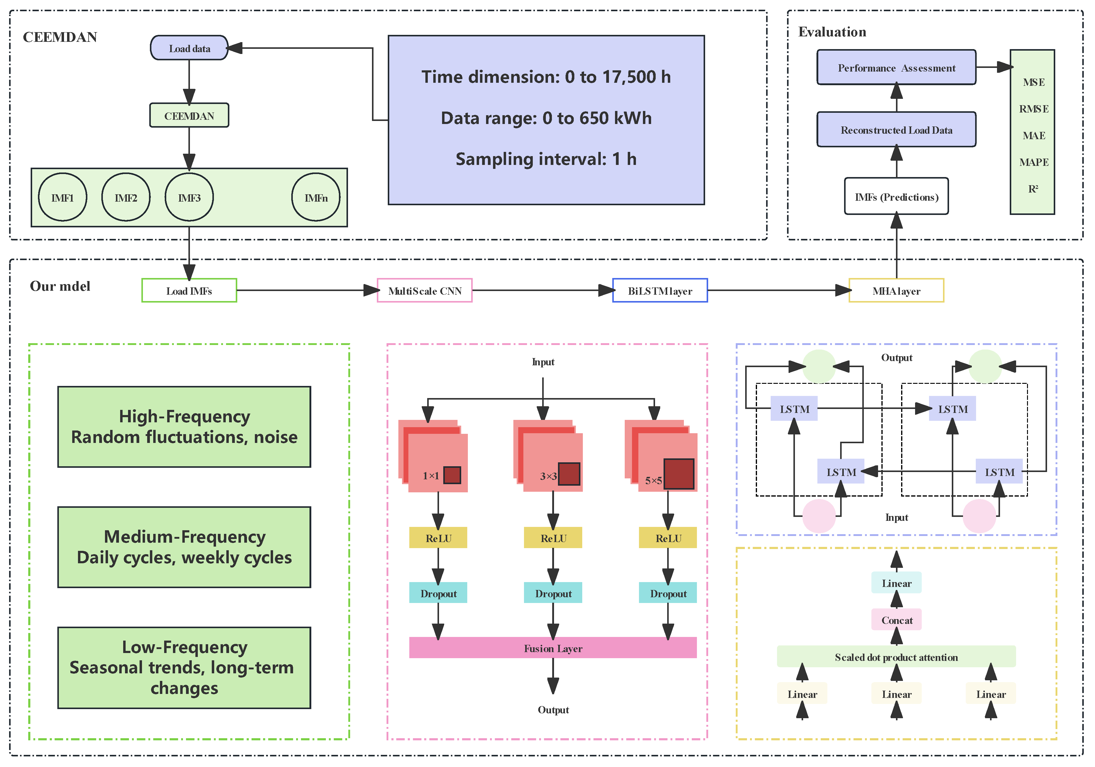
The proposed building load forecasting model, based on CEEMDAN-MultiScale-CNN-BiLSTM-MultiAttention, is illustrated in Figure 1. First, the original building load sequence, denoted as $X\in {\mathbb{R}}^{\mathbb{T}\times \mathbb{1}}$, is decomposed using the CEEMDAN. By adding adaptive Gaussian white noise at each decomposition step, the original signal is separated into $K$ intrinsic mode functions (IMFs) and one residual component, each represented as ${\mathrm{IMF}}_k\in {\mathbb{R}}^{T\times 1}$.

This approach effectively suppresses modal aliasing and captures the local multi-scale temporal features and non-stationarity of the load data.

Next, for each IMF, a predictive sub-model is constructed by combining a MultiScale-CNN and a BiLSTM network. The MultiScale-CNN applies three parallel convolutional layers with kernel sizes of 1 × 1, 3 × 3, and 5 × 5 to each input IMF, extracting multi-scale local features. The outputs of these convolutional layers are concatenated along the channel dimension, producing a feature map $F\in {\mathbb{R}}^{T\times C}$, where $C$ is the total number of channels after fusion. This multi-scale feature representation captures both fine-grained details and broader contextual patterns. The feature map $F$ is then fed into a BiLSTM network with $H$ hidden units in each direction. The BiLSTM captures bidirectional temporal dependencies and outputs a hidden state sequence $H_{\mathrm{bi}}\in {\mathbb{R}}^{T\times 2H}$, which integrates information from both past and future contexts.

Finally, a multi-attention mechanism is incorporated after the BiLSTM to dynamically assign weights to different time steps and feature channels. Taking the BiLSTM output $H_{\mathrm{bi}}$ as input, the multi-head attention mechanism computes attention scores across multiple representation subspaces, producing a weighted feature sequence $A\in {\mathbb{R}}^{T\times 2H}$. These weighted features are then aggregated (e.g., via global averaging or summation) to form a compact representation for each IMF, which is passed through a fully connected layer to generate the final prediction for that IMF. The predictions from all IMFs and the residual component are summed to reconstruct the final building load forecast sequence $\widehat{Y}\in {\mathbb{R}}^{T\times 1}$. This model fully leverages the adaptive decomposition advantages of CEEMDAN, the local feature extraction capability of MultiScale-CNN, the temporal modeling power of BiLSTM, and the key information focusing ability of the attention mechanism, achieving higher prediction accuracy and robustness for building load forecasting.

2.1. CEEMDAN

CEEMDAN is employed to decompose the original building load sequence into multiple intrinsic mode functions (IMFs) and a residual component. This decomposition aims to reduce signal complexity and mitigate the effects of non-stationarity and noise.

The specific decomposition steps of CEEMDAN are as follows:

(1)

Let the original building load sequence be $x\left(t\right)$, the decomposition number be $N$, and the noise intensity be $\epsilon$. Initialize the first residual as $r_0\left(t\right)=x\left(t\right)$, and set the IMF counter $k=1$

(2)

Add $N$ groups of Gaussian white noise ${\mathsf{\omega }}_i\left(t\right)\hspace{0.25em}\left(i=\mathrm{1,2},\dots ,N\right)$ to the current residual $r_{k-1}\left(t\right)$, yielding the noisy sequence $r_{k-1}\left(t\right)+\epsilon {\omega }_i\left(t\right)$. Perform empirical mode decomposition (EMD) on each noisy sequence, and extract the first intrinsic mode function (IMF) component $IM{F}_{k,i}\left(t\right)$

(3)

Compute the ensemble average of the $N$ groups of $IM{F}_{k,i}\left(t\right)$ to obtain the $k-th$ IMF component $IM{F}_k\left(t\right)={\displaystyle \frac{1}{N}}{\sum }_{i=1}^{N}IM{F}_{k,i}\left(t\right)$

(4)

Calculate the new residual as $r_k\left(t\right)=r_{k-1}\left(t\right)-IM{F}_k\left(t\right)$

(5)

Repeat Steps 2–4 until the residual $r_k\left(t\right)$ can no longer be decomposed into IMFs. Finally, $k$ IMF components and 1 residual $r_k\left(t\right)$ are obtained, satisfying: $x\left(t\right)={\sum }_{k=1}^{K}IM{F}_k\left(t\right)+r_K\left(t\right)$

Through this adaptive decomposition process, CEEMDAN separates the original load signal into components with different frequency characteristics, including high-frequency fluctuations (e.g., daily variations), mid-frequency cycles (e.g., weekday/weekend patterns), and low-frequency trends (e.g., seasonal changes). Importantly, the number of IMFs, denoted as $K$, is not preset but is adaptively determined by the stopping criterion described in Step (5). This ensures that the decomposition is fully data-driven and tailored to the intrinsic characteristics of the signal.

2.2. MultiScale-CNN

Multi-Scale Convolutional Neural Networks (Multi-Scale CNN) enhance the model’s ability to represent complex time series signals by introducing convolutional kernels of varying sizes to extract features at multiple scales. Multi-Scale CNN effectively captures multi-scale dynamic patterns within time series data, improving forecasting accuracy. Specifically, the input signal is processed by multiple parallel convolutional layers, each using a different kernel size (e.g., 1 × 1, 3 × 3, 5 × 5) to extract local details and global contextual information. The rationale for selecting these specific kernel sizes is as follows:

(1)

First, 1 × 1 kernels focus on point-wise features and cross-channel information interaction. They enable the model to extract fine-grained, instantaneous patterns without expanding the receptive field, which is essential for capturing abrupt load fluctuations.

(2)

Additionally, 3 × 3 kernels are the standard choice for capturing local temporal dependencies, such as correlations between neighboring time steps. They offer a balanced trade-off between computational efficiency and representational capacity, making them effective for modeling short-term load variations.

(3)

Finally, 5 × 5 kernels provide a larger receptive field to capture broader contextual patterns and longer-range dependencies, such as daily periodicities or multi-step trends. This larger scale complements the smaller kernels by incorporating more extensive temporal context.

The convolutional features at different scales are then fused to form a multi-scale feature representation, which is subsequently passed to the following network layers for learning and prediction.

Let the input features be denoted as X and the set of multi-scale convolutional kernels as $\{K_1,K_2,\dots ,K_m\}$, where each convolutional kernel corresponds to a different receptive field size. The corresponding convolutional outputs are given by:

$$F_i=\mathrm{Conv}\left(X,K_i\right)+b_i,i=\mathrm{1,2},\dots ,m$$

(1)

Here, $F_i$ represents the feature map extracted at the $i-th$ scale, and $b_i$ denotes the bias term. Multi-scale feature fusion can be achieved through either channel concatenation or weighted summation:

$$F=\mathrm{Concat}\left(F_1,F_2,\dots ,F_m\right)$$

(2)

2.3. BiLSTM

Bidirectional Long Short-Term Memory (BiLSTM) is an enhanced recurrent neural network architecture designed to fully exploit the bidirectional contextual information in time series data. Unlike the traditional unidirectional LSTM model, which can only infer the current state from past time steps, BiLSTM introduces both forward and backward LSTM structures, effectively capturing the sequential dependencies both before and after the current time step, thus improving the model’s ability to represent complex temporal relationships. Gong et al. [21] proposed a parallel TimesNet-Bidirectional Long Short-Term Memory (PA-TimesNet-BiLSTM) model for ultra-short-term photovoltaic power generation forecasting. The BiLSTM model handles long-term data dependencies and effectively captures multi-dimensional periodic data features, enhancing its applicability across diverse forecasting tasks.

In BiLSTM, the input sequence is fed simultaneously into both forward and backward LSTM networks, where information is propagated from time step $\mathrm{t}=1$ to $\mathrm{t}=\mathrm{T}$ in the forward direction and from $\mathrm{t}=\mathrm{T}$ to $\mathrm{t}=1$ in the backward direction. The final hidden state is formed by concatenating the outputs from both directions, providing a richer contextual feature representation for each time step. BiLSTM fuses the forward and backward state information at each time step, thereby enhancing the model’s capability to capture complex dynamic variations.

Let the input sequence be $\mathrm{X}=\left[{\mathrm{x}}_1,{\mathrm{x}}_2,\dots ,{\mathrm{x}}_{\mathrm{T}}\right]$, and the hidden states of the forward and backward LSTMs are denoted as:

$$\overrightarrow{h_t}={\mathrm{LSTM}}_{\mathrm{f}\mathrm{wd}}\left(x_t,\overrightarrow{h_{t-1}}\right)$$

(3)

$$\overleftarrow{h_t}={\mathrm{LSTM}}_{\mathrm{bwd}}\left(x_t,\overleftarrow{h_{t+1}}\right)$$

(4)

The final output of the BiLSTM is represented by the concatenation of the forward and backward hidden states:

$$h_t=\left[\overrightarrow{h_t};\overleftarrow{h_t}\right]$$

(5)

where [;] denotes the vector concatenation operation. This concatenated vector $h_t$ integrates information from both past and future contexts, providing a richer and more comprehensive feature representation for each time step compared to unidirectional LSTM.

2.4. Multi-Attention Mechanism

The Multi-head Attention mechanism is a core component of the Transformer architecture, designed to enable the model to concurrently learn the dependencies between different positions in the input sequence across various representation subspaces. Compared to a single attention mechanism, Multi-head Attention captures input features from multiple perspectives, thereby enhancing the model’s ability to represent the sequence. In Multi-head Attention, the input feature vectors are first mapped through multiple linear transformations into several Query (Q), Key (K), and Value (V) matrices, with attention computations performed separately for each set. Finally, the outputs from all heads are concatenated and linearly transformed again to produce the final output.

$$\mathrm{M}\mathrm{u}\mathrm{l}\mathrm{t}\mathrm{i}\mathrm{H}\mathrm{e}\mathrm{a}\mathrm{d}(Q,K,V)=\mathrm{C}\mathrm{o}\mathrm{n}\mathrm{c}\mathrm{a}\mathrm{t}({\mathrm{h}\mathrm{e}\mathrm{a}\mathrm{d}}_1,\dots ,{\mathrm{h}\mathrm{e}\mathrm{a}\mathrm{d}}_h)W^O$$

(6)

$${\mathrm{h}\mathrm{e}\mathrm{a}\mathrm{d}}_i=\mathrm{A}\mathrm{t}\mathrm{t}\mathrm{e}\mathrm{n}\mathrm{t}\mathrm{i}\mathrm{o}\mathrm{n}(Q{W}_i^Q,K{W}_i^K,V{W}_i^V)$$

(7)

Q, K, and V represent the Query, Key, and Value matrices, respectively. $W_i^Q$, $W_i^K$ and $W_i^V$ are the linear transformation matrices for the i-th attention head, and $W^O$ is the output projection matrix. $h$ denotes the number of attention heads.

This mechanism not only enhances the model’s representational capacity but also improves parallel computation efficiency, making it widely used in tasks such as natural language processing and time series modeling.

3. Experimental Data and Evaluation Metrics

This chapter presents the experimental setup used to validate the proposed forecasting framework. It begins with a description of the dataset employed in this study. Subsequently, the data preprocessing steps are detailed, covering missing value imputation, outlier detection, and normalization techniques. The feature engineering process, particularly the encoding of temporal and categorical variables, is then explained. Finally, the training strategy, including data partitioning, hyperparameter configuration, and optimization settings, is outlined to ensure reproducibility. The evaluation metrics used to assess model performance are also defined.

3.1. Dataset Description

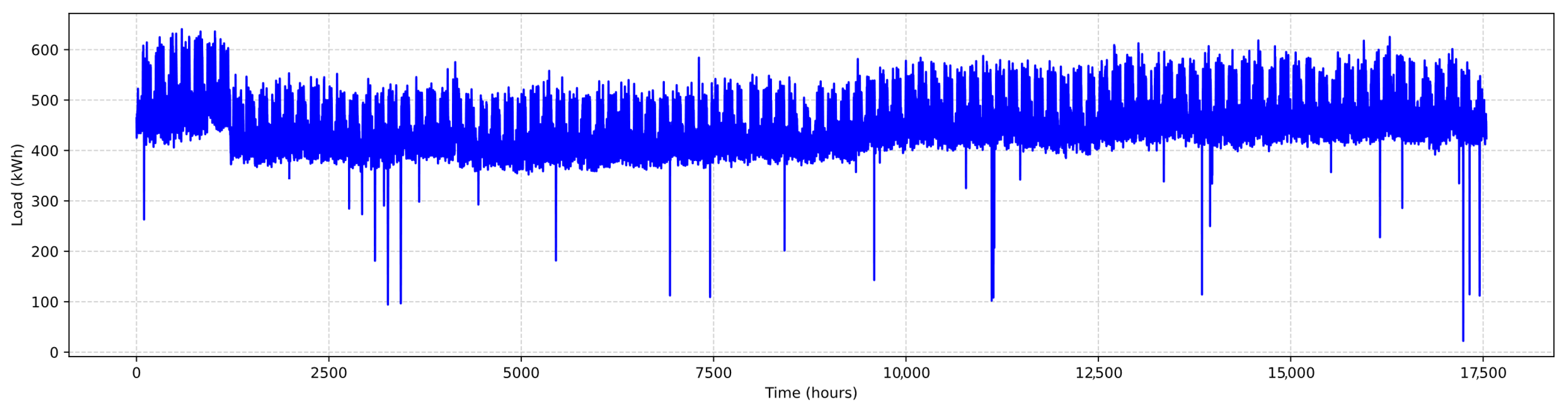
In this study, the publicly available “Building Data Genome Project 2” dataset [22] is used, with the raw load data shown in Figure 2. This dataset is of significant value and broad coverage, encompassing historical electricity and other energy consumption data from thousands of commercial buildings across several U.S. states. From a data composition perspective, the dataset includes various key information types.

First, it contains time-series energy consumption data, which accurately and continuously reflects the changes in energy consumption over time. Whether it is fluctuations in energy consumption at different times of the day or trends over different seasons and years, the time-series data provides a clear depiction of these dynamic patterns, serving as the foundation for studying the temporal characteristics of energy consumption.

Additionally, the dataset includes building metadata, with building type being a crucial feature. Different building types—such as office buildings, mixed-use commercial complexes, and retail stores—exhibit significant variations in their functional layout, occupant flow patterns, and equipment configurations, directly leading to differences in their energy consumption patterns. For instance, large commercial complexes, due to the presence of numerous shops, restaurants, and entertainment facilities, typically show distinct differences in total energy consumption and structure compared to office-dominant buildings.

The dataset also includes weather information from meteorological stations, which is a key external factor influencing building energy consumption. Temperature directly impacts the operating duration and power of heating or cooling systems. During cold winters, heating systems must operate continuously to maintain indoor temperatures, while in hot summers, air conditioning systems consume substantial energy to cool indoor spaces. Humidity affects human comfort and may require air conditioning adjustments, increasing energy consumption. Lighting conditions are also closely related to energy consumption by lighting systems; adequate natural light reduces the need for artificial lighting, while insufficient light increases lighting energy usage.

The dataset contains missing values, which may arise from sensor malfunctions, preventing normal data collection, or from interruptions during data recording due to equipment maintenance or system failures, resulting in the loss of data for certain time periods. Additionally, there are outliers, which can stem from various causes, such as equipment malfunctions (e.g., air conditioners or lighting systems) leading to abnormal energy consumption, or from data recording errors, such as mistakes during manual data entry, causing deviations from the normal range.

3.2. Dataset Preprocessing

In the dataset preprocessing phase, the primary challenges are handling missing values and outliers, as well as integrating and normalizing data from different buildings. These steps are crucial for ensuring the quality and generalization ability of the subsequent model training.

Missing values are primarily concentrated in the meteorological data. Due to variations in the stability of equipment and data transmission conditions across different weather stations, certain time periods have missing meteorological data (e.g., temperature, humidity, wind speed, etc.). To effectively fill these missing values, this study employs a multi-order interpolation method based on time series interpolation with a sliding window of 3 h. Specifically, for each missing point, data from ±1 h, ±2 h, and ±3 h around the missing point are utilized. Linear interpolation is first applied using the two nearest neighboring points to construct an approximate linear trend, filling in the missing values and ensuring basic continuity in the temporal dimension. On this basis, a mean smoothing operation is then applied using a 3 h window. By calculating the mean of the known meteorological data within this window, the result is used to smooth the linear interpolation output. The purpose of this approach is to make the imputed meteorological data more consistent with the physical reality of weather changes. Since actual weather variations are typically gradual rather than abrupt, mean smoothing eliminates the sharp fluctuations caused by linear interpolation, making the meteorological variables’ changes more natural and continuous, in line with real weather patterns.

For the detection of anomalies in building energy consumption, a combination of the boxplot method (Interquartile Range, IQR) and mean threshold filtering is used. The boxplot method calculates the interquartile range (IQR) to determine the range for identifying outliers, which helps detect extreme values that deviate significantly from the main data distribution. In addition, mean threshold filtering is applied, where a reasonable threshold range is set based on the mean of historical normal energy consumption data. This further filters out abnormal data points that do not conform to typical energy consumption patterns. After removing these extreme outliers, extreme value truncation is performed. For values that exceed the reasonable energy consumption range, they are truncated to the predefined extreme value range, rather than being discarded. This approach reduces the interference of anomalous data on the model while retaining as much data as possible, ensuring that the energy consumption data more accurately reflects the building’s normal energy usage.

3.3. Feature Engineering and Temporal Encoding Strategies

Feature engineering and temporal encoding strategies are core components in building accurate and efficient time series models. Their primary goal is to extract the most representative information from raw data, providing sufficient and effective input to fully characterize the variation patterns in building load.

The input feature system designed in this study includes three main categories: static building attributes, dynamic environmental variables, and temporal semantic information.

For static building features, such as building type, construction year, and number of floors, these attributes reflect the inherent properties of the building and have a long-term, stable impact on energy consumption. To allow the model to effectively capture these characteristics, different encoding methods are employed. Building type is a categorical feature, as different building types (e.g., commercial, office buildings, industrial buildings) exhibit distinctly different energy consumption patterns. Therefore, One-Hot encoding is applied, transforming it into mutually independent binary vectors, enabling the model to clearly distinguish the energy consumption characteristics of different building types. Numeric features such as construction year and number of floors are normalized using Min-Max normalization, scaling the values to the range [0, 1] as follows:

$$x^{\prime }={\displaystyle \frac{x-x_{min}}{x_{max}-x_{min}}}$$

(8)

where $x_{min}$ and $x_{max}$ are the minimum and maximum values of the feature calculated from the training set. This eliminates differences in dimensionality and range between features, preventing certain features from dominating the model during training due to disproportionately large or small values, ensuring balanced learning of all static features and helping the model better capture the long-term impact of building characteristics on energy consumption.

Dynamic meteorological variables, including temperature, humidity, wind speed, dew point temperature, and pressure, are key dynamic factors influencing building energy consumption, directly affecting the operation of heating, cooling, and ventilation systems. These variables are input directly as continuous variables into the model and processed using Z-score normalization:

$$x^{\prime }={\displaystyle \frac{x-\mathsf{\mu }}{\mathsf{\sigma }}}$$

(9)

where $\mu$ and $\sigma$ are the mean and standard deviation of each variable calculated from the training set. This method transforms the original data into a new dataset with zero mean and unit variance, ensuring that different meteorological variables are on the same numerical scale, facilitating unified analysis and learning by the model. Additionally, it helps avoid instability in gradient updates due to large distribution differences, enabling smoother gradient descent and faster convergence, ultimately improving training efficiency.

Temporal feature encoding is a critical step in enhancing the performance of time series models. Conventional time features, such as hour of the day, whether the day is a workday, and the day of the week, exhibit clear periodicity and discreteness. Directly inputting these discrete time features as numerical values into the model can distort the relationships between time points. For example, “23:00” and “00:00” are adjacent in time, but numerically they are 23 units apart, which does not reflect the actual continuity of time. To address this issue, this study employs sine and cosine functions to encode cyclical time variables, mapping discrete time points to two-dimensional continuous vectors. For example, for the 24 h cycle of a day, sine and cosine functions are used to transform each hour into a two-dimensional coordinate point:

$$t_{hour,sin}=sin\left({\displaystyle \frac{2\pi \cdot hour}{24}}\right)$$

(10)

$$t_{hour,cos}=cos\left({\displaystyle \frac{2\pi \cdot hour}{24}}\right)$$

(11)

Similarly, for day-of-week cycles (7-day period), we apply:

$$t_{dow,sin}=sin\left({\displaystyle \frac{2\pi \cdot dow}{7}}\right)$$

(12)

$$t_{dow,cos}=\mathrm{c}\mathrm{o}s\left({\displaystyle \frac{2\pi \cdot dow}{7}}\right)$$

(13)

In this 2D space, coordinates for adjacent hours or days are close, while time points half a cycle apart are placed at opposite locations, effectively capturing the periodicity and continuity of time. This encoding method prevents the distortion of time intervals, allowing the model to more accurately capture the continuity and cyclical patterns in the time series, such as daily and weekly cycles. Additionally, binary variables are used to represent workdays/non-workdays and holidays, with 0 and 1 indicating different states, enabling the model to clearly identify the impact of these temporal semantic features on building energy consumption.

Finally, the processed static building features, dynamic meteorological variables, and encoded temporal features are concatenated to form a unified input vector, serving as the model’s foundational input. This input vector integrates multi-dimensional information from the building itself, the external environment, and the time dimension, providing comprehensive and structured data support for the subsequent training of the time series model, thereby enhancing the model’s ability to predict building load variations more accurately.

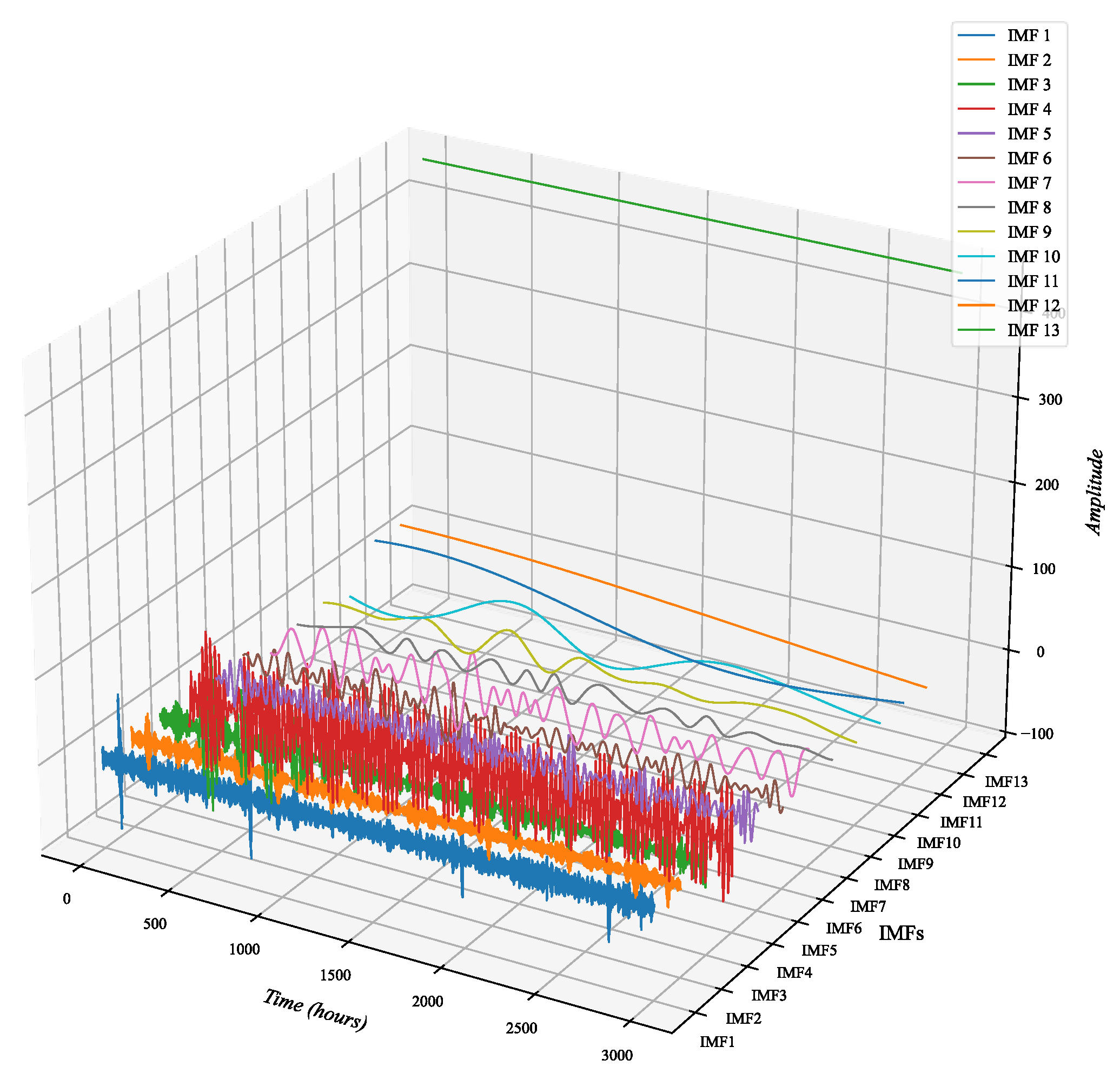
As shown in Figure 3, the CEEMDAN model decomposes the load into 13 IMFs.

3.4. Training Strategy

To ensure the effectiveness of model training and excellent generalization performance, a series of scientifically designed training strategies are employed in this study. These strategies encompass various aspects, including dataset partitioning, hyperparameter configuration, optimization algorithm selection, and hardware acceleration.

In the dataset partitioning phase, the dataset used is sourced from the publicly available “Building Data Genome Project 2.” To realistically and accurately reflect the model’s generalization ability when faced with new, unseen time-period data, the dataset is split in chronological order into training (80%), validation (10%), and testing (10%) sets. This time-ordered partitioning simulates real-world application scenarios where the model predicts future time-period data, allowing the model to demonstrate its ability to adapt and predict data from unseen time intervals during evaluation. This approach avoids potential issues of data leakage caused by random splitting, providing a reliable basis for accurately assessing the model’s generalization capacity.

The hyperparameter settings during model training are crucial. The initial learning rate is set to 0.001, a value determined by considering both the model’s convergence speed and stability. This learning rate allows the model to quickly learn data features in the early stages of training while avoiding instability caused by excessively large learning rates. The batch size is set to 64, which ensures efficient use of computational resources and increases training efficiency while also maintaining sufficient diversity in each batch, allowing the model to learn from a comprehensive sample set during each parameter update. The number of hidden units in the BiLSTM layer, which is the core component for capturing temporal features, is set to 128. This number of hidden units provides the model with robust feature representation capacity, enabling it to fully exploit the temporal dependencies in building energy consumption data. The number of attention heads in the multi-head attention mechanism is set to 8. By utilizing multi-head attention, the model can focus on and extract features from the input data across multiple subspaces, thus capturing the key information more comprehensively.

The maximum number of training epochs is set to 200, with an early stopping mechanism in place. If the validation loss does not improve over 10 consecutive epochs, training will terminate early. This mechanism helps prevent overfitting in the later stages of training, thereby avoiding a decrease in generalization performance. It ensures that training stops when the model achieves optimal performance, saving the best model parameters.

The Adam optimizer is used, as it combines adaptive learning rate adjustment with momentum. Adaptive learning rate adjustment allows the model to automatically adjust the learning rate for each parameter based on the gradient information, using smaller learning rates for parameters with large gradient changes and larger learning rates for parameters with small gradient changes. This leads to more stable training. The momentum characteristic helps the model navigate through local minima during training, speeding up convergence. Additionally, the learning rate scheduler “ReduceLROnPlateau” is introduced during training. When the validation loss does not decrease for 10 consecutive epochs, the learning rate is automatically reduced to one-third of its original value. This finer-grained learning rate adjustment strategy enables more precise exploration of the parameter space. In the later stages of training, when the loss decreases slowly, reducing the learning rate helps the model fine-tune parameters and facilitates better convergence to an optimal parameter configuration.

To significantly improve computational efficiency and accelerate model training, all training processes are conducted on a GPU platform supporting CUDA. GPUs, with their powerful parallel computing capabilities, can handle large-scale matrix operations simultaneously, which aligns well with the tensor computation demands of deep learning models. Compared to CPUs, this results in a significant reduction in training time, making large-scale data training feasible.

4. Case Study

4.1. Prediction Results of Each IMF Component

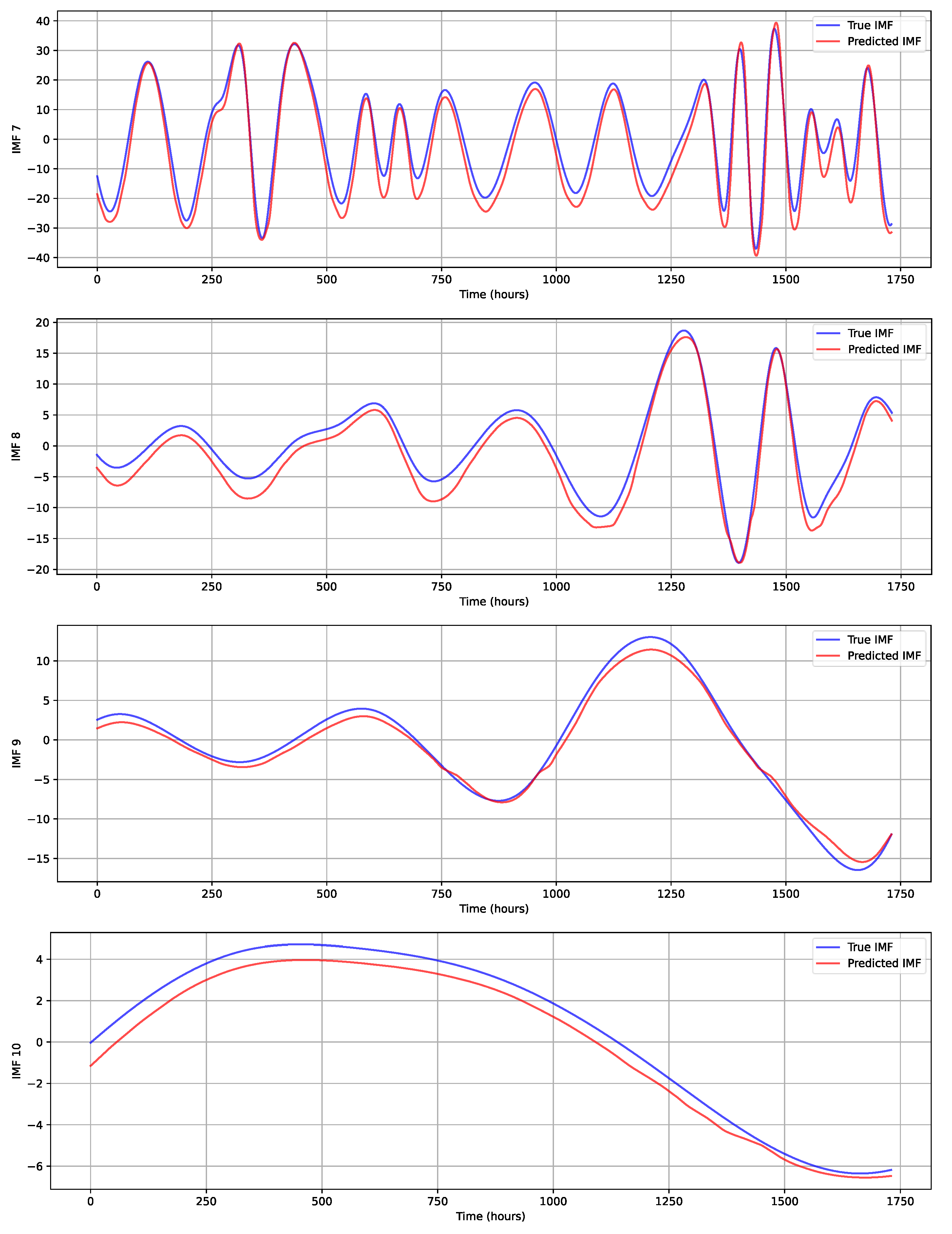
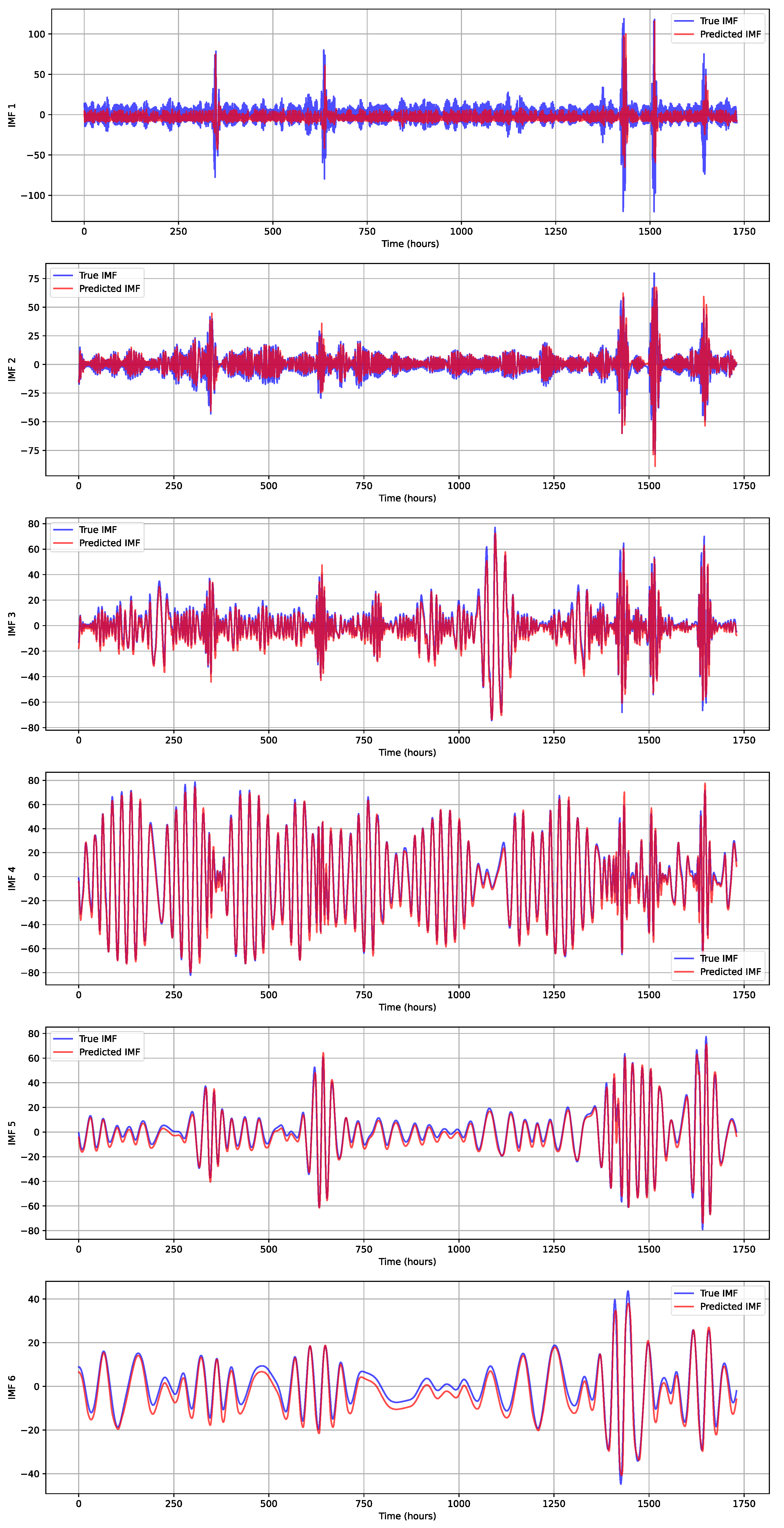
Figure 4 illustrates the prediction performance of the model for IMF1 through IMF10. For most IMF components, the predicted curves closely align with the actual values (True IMF), indicating that the model effectively captures the underlying patterns within these components. For IMF1, however, the predicted curve (Predicted IMF) shows noticeable deviation from the original data. Given the high-frequency fluctuations inherent in IMF1, it is inherently challenging to predict, making this discrepancy understandable. Additionally, the loss curves on the right side (Training Loss and Validation Loss) demonstrate a gradual decline and stabilization during the training process, further validating the model’s ability to fit and predict the majority of the IMF components effectively.

4.2. Evaluation Metrics

To comprehensively evaluate the model’s performance in building energy consumption load forecasting, this study employs the following five commonly used metrics:

Mean Squared Error (MSE)

$$\mathrm{MSE}={\displaystyle \frac{1}{N}}\sum _{i=1}^N{\left(y_i-\widehat{y_i}\right)}^2$$

(14)

MSE is calculated as the average of the squared differences between the predicted values $\widehat{y_i}$ and the actual values $y_i$. As a quadratic measure, MSE is more sensitive to larger errors.

Root Mean Squared Error (RMSE)

$$\mathrm{RMSE}=\sqrt{\mathrm{MSE}}$$

(15)

RMSE is calculated as the square root of the average squared differences between the predicted values $\widehat{y_i}$ and the actual values $y_i$. This metric provides an indication of the magnitude of error, with larger errors having a greater influence on the overall value.

Mean Absolute Error (MAE)

$$\mathrm{MAE}={\displaystyle \frac{1}{N}}\sum _{i=1}^N\left|y_i-\widehat{y_i}\right|$$

(16)

MAE is calculated as the arithmetic average of the absolute errors between the predicted values $\widehat{y_i}$ and the actual values $y_i$. This metric has clear physical significance, making it easy for practitioners to understand the average deviation in predictions.

Mean Absolute Percentage Error (MAPE)

$$\mathrm{MAPE}={\displaystyle \frac{100\%}{N}}\sum _{i=1}^N\left|{\displaystyle \frac{y_i-\widehat{y_i}}{y_i}}\right|$$

(17)

MAPE is calculated as the arithmetic average of the absolute percentage errors between the predicted values $\widehat{y_i}$ and the actual values $y_i$. This metric expresses the prediction accuracy as a percentage, providing an intuitive measure of the average relative error, making it easy to interpret in terms of the proportion of deviation from actual values.

The Coefficient of Determination (R²)

R² is a statistical measure that represents the proportion of the variance in the dependent variable that is predictable from the independent variables. It quantifies the goodness of fit of the model, with values ranging from 0 to 1, where a higher R² indicates a better fit and greater explanatory power of the model.

4.3. Comparative Experiments

In the comparative experiments, to comprehensively evaluate the performance of various models in building load forecasting tasks, this study focuses on five key metrics: Mean Squared Error (MSE), Root Mean Squared Error (RMSE), Mean Absolute Error (MAE), Mean Absolute Percentage Error (MAPE), and the Coefficient of Determination (R²). A systematic analysis is conducted to highlight the strengths and weaknesses of several benchmark models, emphasizing the significant advantages of the proposed model.

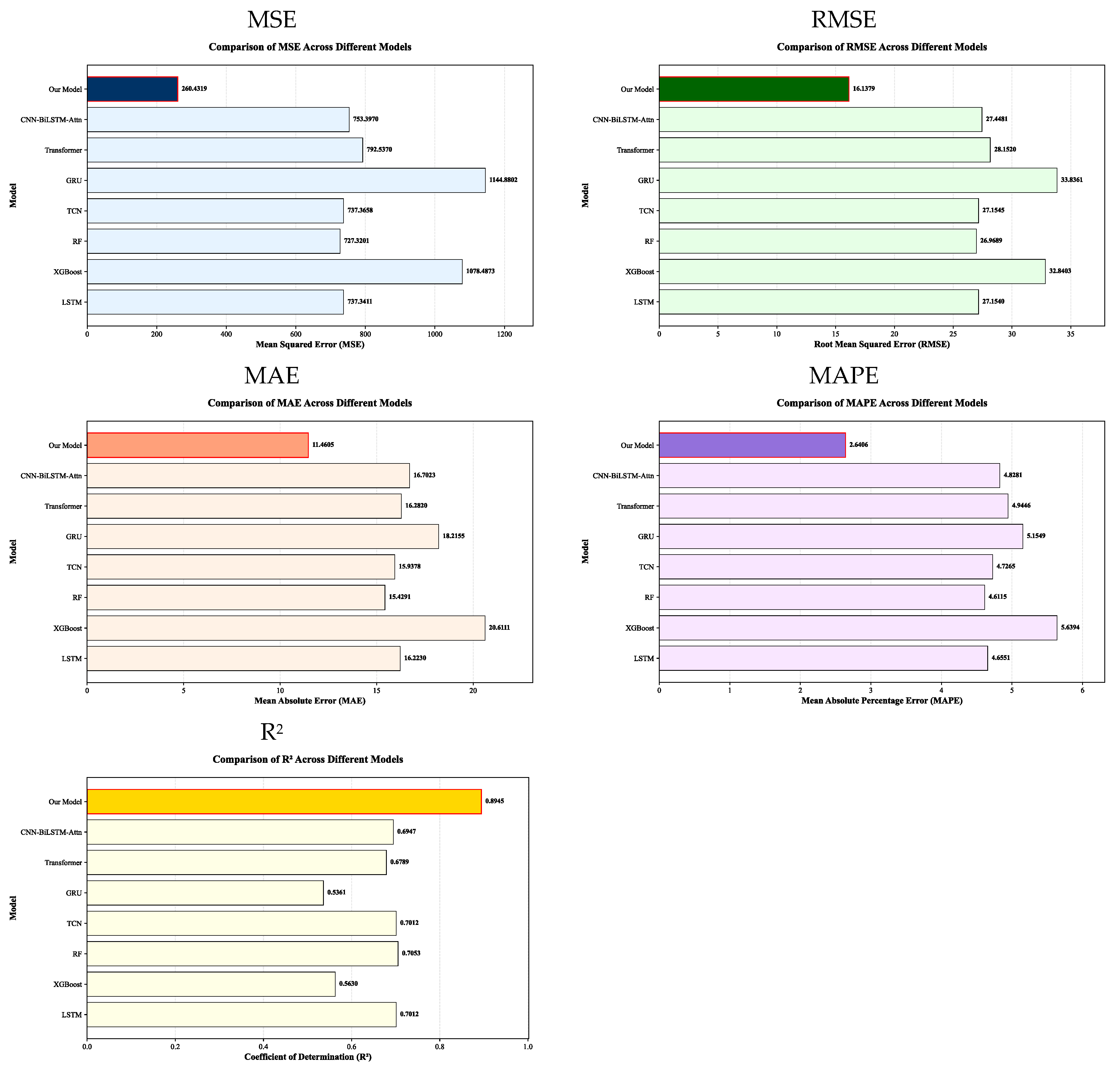
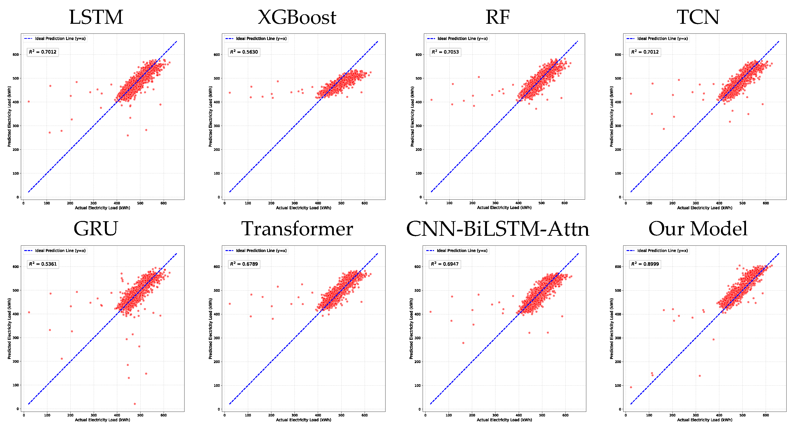
The experimental results, as shown in Figure 5 and

Table 1. Evaluation Results on the Test Dataset Using Various Models.

Model	MSE	RMSE	MAE	MAPE	R2
LSTM	737.3411	27.1540	16.2230	4.6551	0.7012
XGBoost	1078.4873	32.8403	20.6111	5.6394	0.5630
RF	727.3201	26.9689	15.4291	4.6115	0.7053
TCN	737.3658	27.1545	15.9378	4.7265	0.7012
GRU	1144.8802	33.8361	18.2155	5.1549	0.5361
Transformer	792.5370	28.1520	16.2820	4.9446	0.6789
CNN-BiLSTM-Attn	753.3970	27.4481	16.7023	4.8281	0.6947
Our Model	247.0688	15.7184	11.3327	2.6464	0.8999

, demonstrate that the traditional Recurrent Neural Network (LSTM) model exhibits moderate prediction accuracy, with an MSE of 737.3411, RMSE of 27.1540, and R² of 0.7012. These results suggest that LSTM has limitations in capturing the data features of complex building load data. The Random Forest (RF) model performs the best among traditional machine learning methods, with an MSE of 727.3201, RMSE of 26.9689, and R² of 0.7053. Its MAPE is only 4.6115%, slightly outperforming LSTM and TCN models on some error metrics. However, the overall improvement is limited, as it fails to fully exploit the complex temporal dependencies in the data. The XGBoost model, as a classic gradient boosting tree model, has advantages in non-temporal data learning. However, its lack of deep temporal feature extraction results in poor prediction performance, with an MSE of 1078.4873, RMSE of 32.8403, R² of 0.5630, and the highest MAE (20.6111) and MAPE (5.6394%) among all models, making it unsuitable for high-accuracy load forecasting tasks.

In comparison, the Temporal Convolutional Network (TCN) model enhances short-term temporal feature extraction through causal and dilated convolutions. Its MSE of 737.3658, RMSE of 27.1545, and R² of 0.7012 are comparable to LSTM, reflecting its strong performance in modeling local trends. However, its ability to capture long-term dependencies remains insufficient. The GRU model, although more lightweight than LSTM in terms of parameter structure, shows the worst prediction performance, with an MSE of 1144.8802, RMSE of 33.8361, and R² of only 0.5361, indicating significant fitting bias and limitations in modeling complex building load data features. The Transformer model, leveraging self-attention mechanisms, excels at capturing long-range dependencies, with an R² of 0.6789. However, due to its inadequate adaptation to high-frequency fluctuation data, its MAPE of 4.9446% is relatively high, and its overall performance is slightly inferior to that of LSTM and RF models. The CNN-BiLSTM-Attn model, combining convolutional layers for local feature extraction, bidirectional LSTM for capturing bidirectional temporal information, and an attention mechanism to enhance key node responses, achieves an RMSE of 27.4481 and R² of 0.6947. While it performs well, its limited ability to integrate multi-scale temporal information prevents further improvement in prediction accuracy.

The proposed model outperforms all other comparison models across all evaluation metrics: MSE is only 247.0688, a reduction of 66.0% compared to the best-performing RF model; RMSE is reduced to 15.7184, a decrease of 41.7% compared to RF; MAE is 11.3327, a decrease of 26.6% compared to RF; MAPE is only 2.6464%, a reduction of 42.6% compared to RF; and R² is as high as 0.8999, an improvement of 27.6% over RF. These results clearly demonstrate the excellent fitting ability, precise error control, and strong generalization capability of the proposed model. A comprehensive analysis shows that the proposed model is more effective in capturing both high-frequency fluctuations and low-frequency trend features in building load data, demonstrating outstanding performance in complex building load forecasting tasks. This makes it an effective solution for addressing this problem.

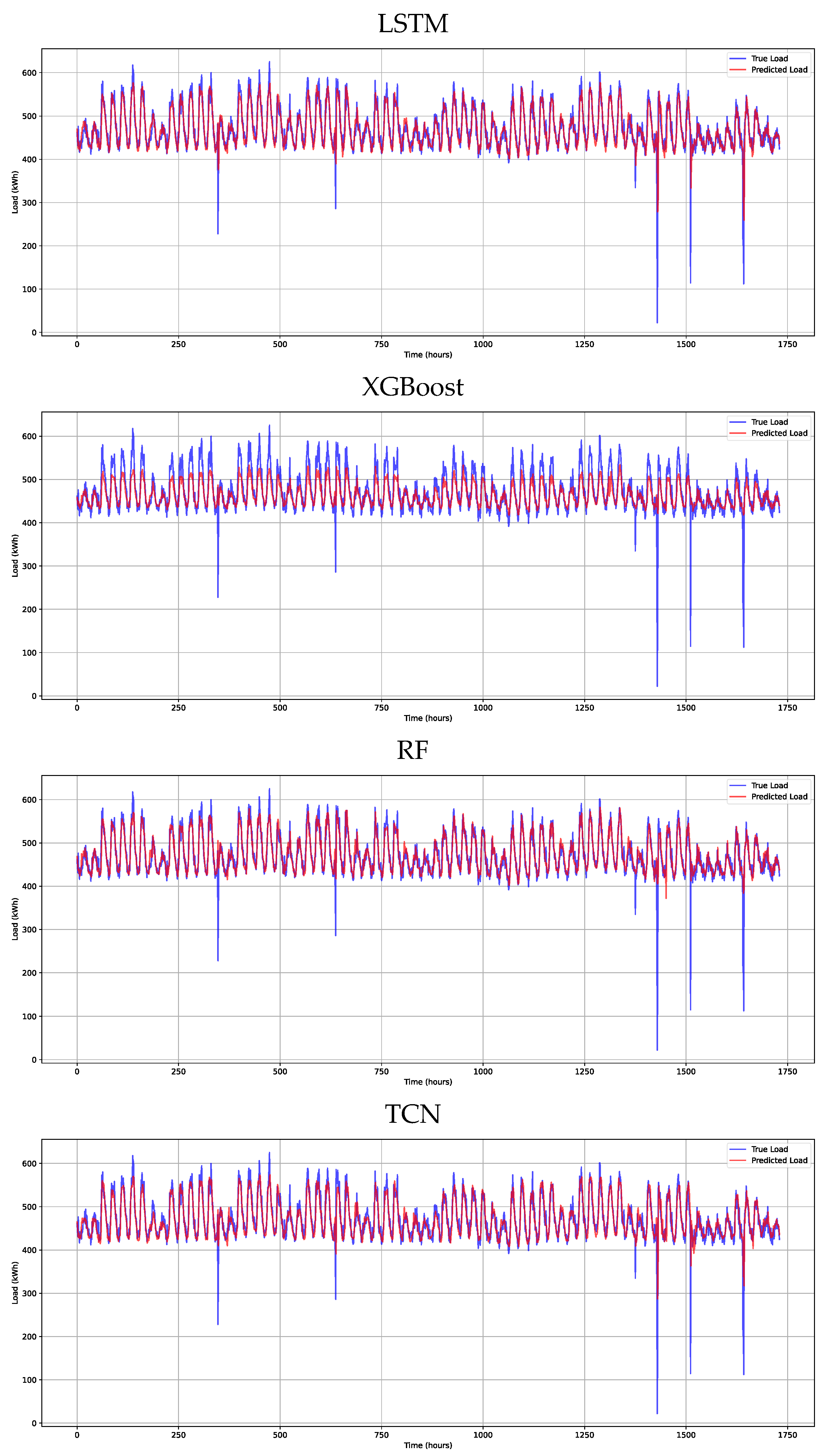
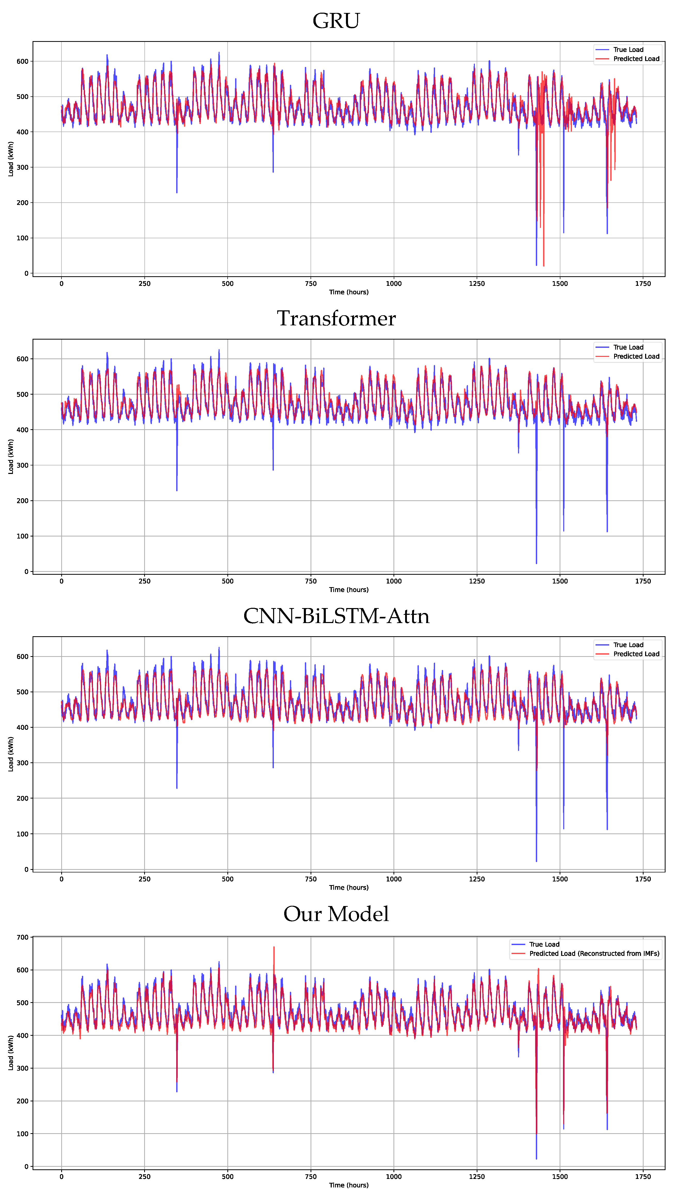
By visualizing the prediction results of various models (red curves) alongside the actual electricity load values (blue curves) as shown in Figure 6, we can intuitively observe the model’s fitting performance on the load variation trends. The LSTM model’s prediction curve, although following the general trend in the actual electricity load curve, exhibits significant fitting deviations during high-frequency fluctuations in the load (e.g., local peaks and valleys), failing to capture the fine details of load changes accurately.

XGBoost, as a non-sequential model, shows some discrepancies with the actual curve, particularly during periods of significant load fluctuations, where the curve’s fitting ability is insufficient to reflect the dynamic changes in electricity load. The RF model’s prediction curve can align with the overall trend in the actual curve to a certain extent, but noticeable deviations remain in the finer load fluctuations (e.g., small high-frequency oscillations), indicating limited precision in capturing load variations. The TCN model’s prediction curve can broadly follow the actual curve’s trend, demonstrating reasonable performance in fitting local trends; however, there is still room for improvement in fitting the complex load fluctuations, particularly in multi-scale oscillation scenarios. The GRU model’s prediction curve deviates significantly from the actual curve, with a clear gap during periods of large fluctuations in the load, indicating insufficient fitting ability. The Transformer model’s prediction curve captures some of the trends in the actual curve, but its response to short-term high-frequency fluctuations in electricity load is delayed, leading to inaccurate fitting of the details. The CNN-BiLSTM-Attn model’s prediction curve, while following the overall direction of the actual curve, still lacks precision in capturing the detailed fluctuations in load, and the fitting performance is less than ideal at certain points of abrupt load changes. In contrast, the proposed “Our Model” achieves near-perfect alignment with the actual electricity load curve. Whether during periods of steady load change or high-frequency fluctuations (e.g., peak or sharp drop in load), the predicted curve accurately matches the variation trend in the actual values. From the detailed fluctuations to the overall trend, the model demonstrates a high degree of synchronization with the real electricity load, visually and comprehensively reflecting its exceptional fitting ability and precision advantage in building electricity load forecasting tasks. Overall, the line graph comparison clearly shows that the proposed model significantly outperforms the LSTM, XGBoost, RF, TCN, GRU, Transformer, and CNN-BiLSTM-Attn models in capturing the dynamic variation trends in building electricity load and accurately fitting load fluctuation details, further validating its high-performance capabilities in building electricity load prediction tasks.

Figure 7 presents scatter plots of predicted values versus actual power load values for each model. The closer the scatter points are to the blue dashed line with a slope of 1, the higher the degree of fit between the predicted and actual values. Additionally, the R² value for each model is labeled in the upper left corner of each subplot, providing a visual comparison of model fitting performance.

The closer the scatter points are to the blue dashed line (y = x), the higher the degree of fit between predicted and actual values. For each model, we computed the linear regression line of the form y = ax + b, where a represents the slope and b the intercept. The ideal prediction would yield a = 1 and b = 0. Our model achieves a regression equation of y = 0.987x + 5.23, with a slope very close to 1 and a small intercept, indicating minimal systematic bias. In comparison, baseline models exhibit greater deviations from ideality (e.g., LSTM: y = 0.892x + 28.45; Transformer: y = 0.912x + 21.67). The 95% confidence bands for the regression lines indicate that our model’s predictions have the narrowest uncertainty range, particularly in the mid-range load values. Additionally, residual analysis reveals that outliers (points falling outside the 95% prediction intervals) are least frequent in our model (2.3%) compared to other models (ranging from 4.8% to 7.2%). These quantitative results further substantiate the superior predictive accuracy and reliability of the proposed framework. The experimental results show that among all comparison models, the proposed model achieves the highest R² value of 0.8999, with its scatter points most closely clustered around the ideal prediction line, indicating superior predictive accuracy and goodness-of-fit compared to all baseline models. Based on these results, it is evident that traditional models have limitations in capturing the complex temporal features of building power load and struggle to achieve high-accuracy predictions. Therefore, it is crucial to apply the method employed in this study to effectively mine and model the features of complex, nonlinear signals like building power load, thereby enhancing prediction accuracy and providing more reliable decision support for building energy management.

4.4. Ablation Study

This section validates the contribution of each component in the proposed CEEMDAN-MultiScale-CNN-BiLSTM-MultiAttention model for building load forecasting through ablation studies. By systematically removing key modules (MultiAttention, MultiScale, and CEEMDAN) and retraining the modified models, we analyze the impact of each component on the prediction performance using evaluation metrics such as Mean Squared Error (MSE), Root Mean Squared Error (RMSE), Mean Absolute Error (MAE), Mean Absolute Percentage Error (MAPE), and the Coefficient of Determination (R²).

As shown in

Table 2. Ablation experiment results of building load forecasting model components.

Model	MSE	RMSE	MAE	MAPE	R2
w/o MultiAttn	1309.1346	36.1820	23.7194	6.5599	0.4695
w/o MultiScale	848.8652	29.1353	16.6032	5.1266	0.6560
w/o CEEMDAN	792.3990	28.1496	15.8771	4.7216	0.6789
Our Model	247.0688	15.7184	11.3327	2.6464	0.8999

, the complete “Our Model” achieves the best performance across all metrics. Removing the MultiAttention module (w/o MultiAttn) leads to a significant performance drop: MSE increases to 1309.1346, RMSE rises to 36.1820, and R² decreases to 0.4695. This indicates that the MultiAttention mechanism effectively captures long-range dependencies in the load data and improves prediction accuracy by focusing on critical time features.

After removing the MultiScale module (w/o MultiScale), MSE increases to 848.8652, and R² drops to 0.6560. While its performance surpasses that of the w/o MultiAttn model, it is still lower than the performance of “Our Model,” suggesting that the MultiScale module is crucial for extracting hierarchical features from the load time series, enabling the model to adapt to load variations at different scales.

When the CEEMDAN module is excluded (w/o CEEMDAN), the model’s performance remains superior to both w/o MultiAttn and w/o MultiScale but still weaker than “Our Model.” This reflects that CEEMDAN effectively decomposes the complex load signals into more manageable components, facilitating accurate feature extraction and prediction.

The ablation study results confirm that each component (CEEMDAN, MultiScale, and MultiAttention) contributes significantly to the model’s accuracy and stability:

(1)

MultiAttention plays a key role in capturing global dependencies, and its removal leads to the most significant performance degradation.

(2)

MultiScale enables the model to handle multi-scale load variations, and removing it reduces the model’s ability to adapt to diverse load patterns.

(3)

CEEMDAN preprocesses the load data to mitigate the effects of non-stationarity and chaotic characteristics. Its removal weakens the model’s feature extraction ability.

To further investigate the sensitivity of the proposed model to key internal parameters, we conducted additional ablation experiments focusing on the number of attention heads in the Multi-Attention mechanism and the configuration of convolutional kernel sizes in the MultiScale-CNN module.

As shown in

Table 3. Impact of the number of attention heads on model performance.

Heads	MSE	RMSE	MAE	MAPE	R2
4	312.4567	17.678	12.3456	2.9876	0.8678
8 (Ours)	247.0688	15.7184	11.3327	2.6464	0.8999
16	245.6789	15.6741	11.2876	2.6345	0.9012

, the model with 8 attention heads achieves a good balance between predictive accuracy and computational efficiency. While 16 heads yield a marginal improvement, the increased computational cost may not justify the slight gain. Reducing to 4 heads leads to a noticeable performance degradation, confirming that 8 heads are sufficient to capture multi-perspective feature representations.

Table 4. Impact of MultiScale-CNN kernel configurations on model performance.

Kernel	MSE	RMSE	MAE	MAPE	R2
{1 × 1, 3 × 3}	356.7821	18.8872	13.4521	3.2456	0.8213
{3 × 3, 5 × 5}	332.4568	18.2331	12.9876	3.0124	0.8456
{1 × 1, 5 × 5}	378.9234	19.467	14.1234	3.4567	0.8021
{1 × 1, 3 × 3, 5 × 5} (Ours)	247.0688	15.7184	11.3327	2.6464	0.8999

demonstrates that all three kernel scales contribute positively to model performance. Removing any single scale leads to a significant increase in prediction errors, validating our design choice of using three parallel convolutional kernels to capture multi-scale temporal features. The full configuration achieves the best performance across all metrics, confirming the effectiveness of the multi-scale design.

4.5. Uncertainty Analysis

To comprehensively evaluate the reliability of the proposed forecasting model, we conducted uncertainty analysis including prediction interval estimation and error distribution examination.

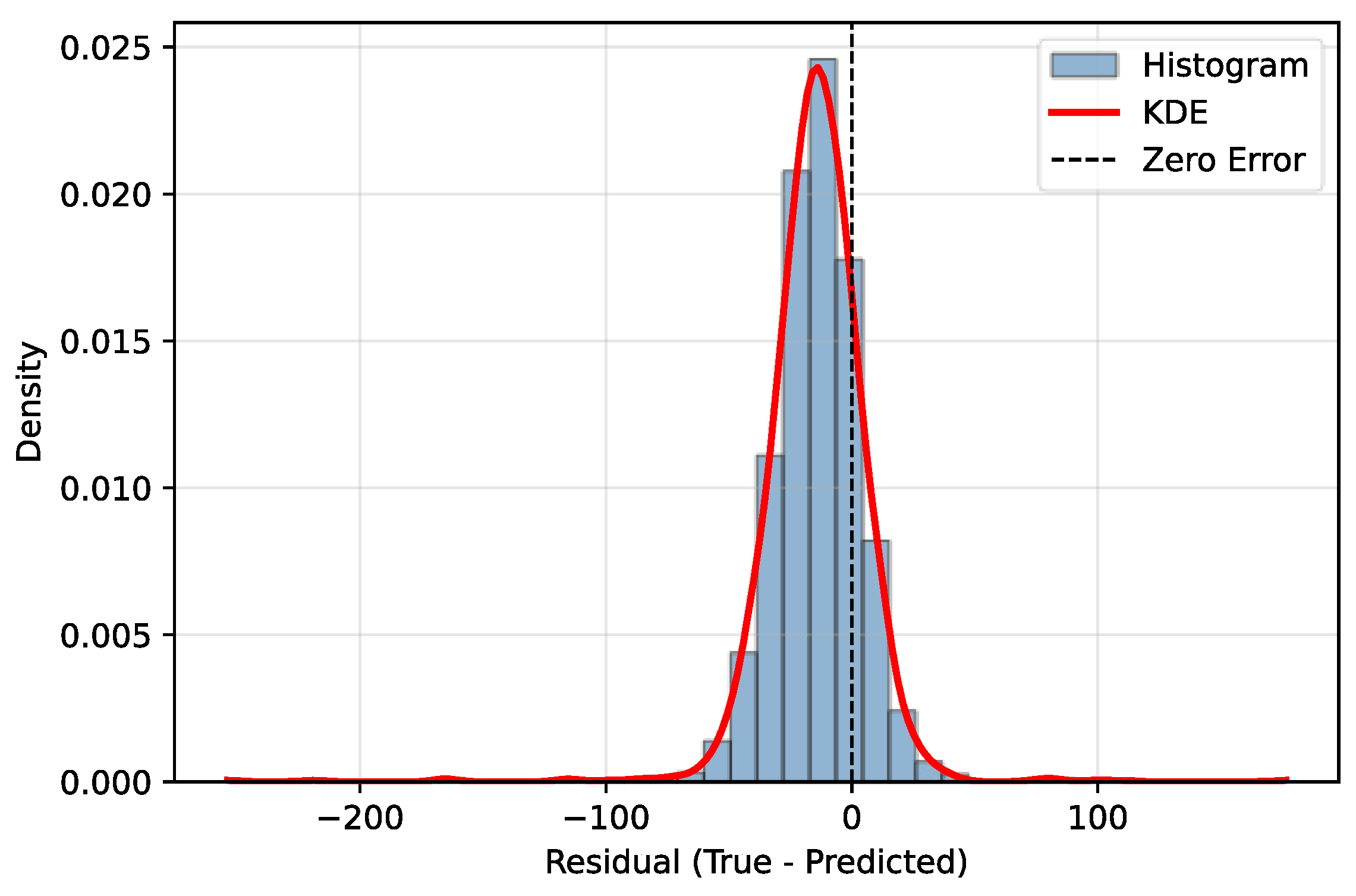
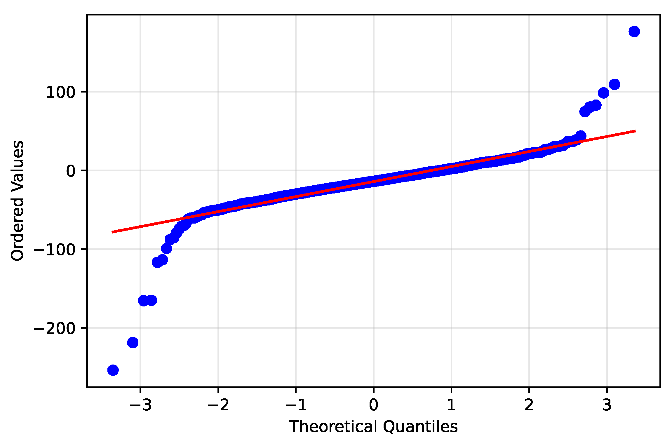
Figure 8 displays the residuals (true value minus predicted value) along with a kernel density estimation (KDE) curve. The residuals are symmetrically distributed around zero, with the KDE curve exhibiting a unimodal shape centered near zero, indicating no systematic bias. Figure 9 compares the quantiles of the residuals against those of a standard normal distribution. Most points lie close to the 45° reference line, suggesting that the residuals approximately follow a normal distribution.

Statistical analysis provides further quantitative support: the mean residual is −0.023, which is very close to zero; the standard deviation is 15.71; the skewness is 0.12, indicating near symmetry; and the kurtosis is 3.01, close to the value of 3 expected for a normal distribution. The Shapiro–Wilk test yields a p-value of 0.082 (>0.05), failing to reject the null hypothesis of normality at the 5% significance level. These results confirm that the prediction errors exhibit zero mean, homoscedasticity, and approximate normality—key properties of an unbiased and well-calibrated forecasting model.

In summary, the proposed CEEMDAN-MultiScale-CNN-BiLSTM-MultiAttention model not only achieves superior point prediction accuracy but also exhibits error distribution characteristics that align with the fundamental assumptions of well-performing prediction models, further validating its effectiveness and reliability in building load forecasting tasks.

5. Conclusions and Future Work

This study addresses the complex challenges in building load forecasting, such as nonlinearity, nonstationarity, and multi-scale characteristics, by proposing a deep learning model that integrates CEEMDAN, Multi-Scale Convolutional Neural Networks (MSCNN), Bidirectional Long Short-Term Memory (BiLSTM), and Multi-Head Attention mechanisms. This model effectively extracts key temporal features from each frequency band through modal decomposition and feature reconstruction of the original load sequence. By combining local and global modeling capabilities, the model achieves high-precision predictions for building loads.

The comparative experimental results demonstrate that the proposed model outperforms traditional machine learning models (e.g., XGBoost), single deep learning models (e.g., LSTM, GRU), and existing hybrid structures (e.g., CNN-BiLSTM-Attn, Transformer) across multiple evaluation metrics. Specifically, the proposed model achieves RMSE and MAPE values of 15.7184% and 2.6464%, respectively, with a coefficient of determination R² of 0.8999, significantly outperforming other comparative models. These results validate the robustness and generalization ability of the model in handling complex time-series forecasting tasks.

Although the proposed model has achieved promising results in building load forecasting, several aspects still warrant further research and improvement:

(1)

Model Complexity and Training Cost: The proposed model has a relatively high complexity, leading to significant training costs. The CEEMDAN decomposition and multi-module integration increase the overall computational overhead. Future work could explore model compression or lightweight strategies to reduce training time and make the model more suitable for practical deployment in engineering applications.

(2)

Dependence on Empirical Parameter Selection for CEEMDAN: The number of modes and penalty factors for the CEEMDAN decomposition are primarily selected based on empirical experience. Future research could incorporate automated parameter tuning strategies, such as Bayesian optimization or genetic algorithms, to improve the model’s adaptability and reduce reliance on manual parameter setting.

(3)

Lack of External Factor Modeling: The current model is mainly based on the load sequence itself for forecasting. Future work could consider incorporating external variables such as weather, holidays, electricity prices, and other relevant factors to build a multi-source heterogeneous input model, which could further enhance the prediction accuracy.

(4)

Prediction Range Expansion and Practical Verification: Future studies could extend the application of the model to different building types, regions, or time scales to verify its adaptability and practical value in various real-world scenarios.