Calculation of Buffer Zone Size for Critical Chain of Hydraulic Engineering Considering the Correlation of Construction Period Risk

Abstract

Due to their large scale, long duration, complex geological conditions, and multiple stakeholders, water conservancy engineering projects are subject to diverse, interrelated, and uncertain risk factors that affect the construction timeline. Traditional critical chain buffer calculation methods, such as the cut-and-paste method and the root variance method, typically assume the independence of risks, which limits their effectiveness in addressing schedule delays caused by correlated risk events. To overcome this limitation, this paper proposes a novel critical chain buffer calculation approach that explicitly incorporates risk correlation analysis. A fuzzy DEMATEL-ISM-BN model is employed to systematically identify the interrelationships and influence pathways among schedule risk factors. Bayesian network inference is then used to quantify the overall occurrence probability while accounting for risk correlations. By integrating critical chain management theory, risk impact coefficients are introduced to improve the traditional root variance method, resulting in a buffer calculation model that captures interdependencies among schedule risks. The effectiveness of the proposed model is validated through a case study of the X Pumped Storage Power Station. The results indicate that, compared with conventional methods, the proposed approach significantly enhances the robustness of project schedule planning under correlated risk conditions while appropriately increasing buffer sizes. Consequently, the adaptability and reliability of schedule control are improved. This study provides novel theoretical tools and practical insights for schedule risk management in complex engineering projects.

1. Introduction

In the field of project management, the Critical Chain Method (CCM) is a widely recognized approach for project planning and execution. By incorporating mechanisms such as project buffers and feeding buffers, CCM effectively addresses inherent task uncertainties and mitigates the impact of human factors, including the “student syndrome.” Determining appropriate buffer sizes is crucial for minimizing planned project duration while maximizing the probability of on-time completion. Consequently, buffer sizing represents an issue of substantial theoretical interest and practical significance.

The development of buffer estimation methods has progressed from empirical simplifications to increasingly sophisticated approaches. Early representative methods include the cut-and-paste technique proposed by Goldratt et al. [1], which defines the project buffer as half the sum of the safety times of activities on the critical chain, and Newbold’s [2] root variance method, which is derived from the central limit theorem. Subsequent studies extensively examined the applicability and rationality of these foundational approaches. For instance, Herroelen et al. [3,4], based on monitoring data from projects of different scales, found that although the cut-and-paste method is computationally simple, it tends to produce overly conservative buffers and is more suitable for small-scale projects. Hoel et al. [5] employed Monte Carlo simulation to determine buffer sizes as the deviation between completion durations at specified confidence levels and the mean duration, thereby reducing dependence on managerial judgment. In recent years, research on buffer estimation has shifted toward more multidimensional and refined methodologies. On the one hand, scholars have sought to more accurately characterize the fuzziness and uncertainty of activity durations. Kołodziej et al. [6] applied fuzzy logic models to buffer estimation to reduce overall project duration, while Fatemeh et al. [7] used triangular interval fuzzy sets to flexibly quantify activity uncertainty. Li et al. [8] further explored data-driven approaches for dynamic buffer adjustment. On the other hand, the research scope has expanded to incorporate multiple constraints, including resources, information, and human factors. Wu et al. [9] improved scheduling efficiency in multi-project environments by jointly optimizing resource and buffer allocation. Nie et al. [10,11,12] conducted a series of studies integrating multi-objective and multi-resource constraints with relay potential, various forms of information entropy, and flexible resource substitution efficiency in buffer zones. Zhang Junguang et al. [13,14] introduced the concepts of resource time value and activity elasticity to guide the configuration and consumption of resource buffers. Huang Jianwen et al. [15] proposed a buffer setting method that explicitly considers resource flexibility, while Zhang Junguang et al. [16] further developed a milestone-based phased buffer monitoring strategy from the perspective of activity- and phase-level risk measurement. These studies have substantially enriched the theoretical and methodological foundations of buffer management. However, a common limitation of these mainstream approaches is their implicit assumption that the risk factors affecting project duration are independent or can be linearly aggregated. Multi-criteria decision analysis (MCDA) methods are widely used in engineering risk studies to rank the importance of risk factors and identify priorities, owing to their ability to integrate multidimensional evaluation information. However, MCDA methods generally yield static weights or ranking results, which limits their ability to capture causal dependencies among risk factors and to represent probabilistic risk propagation mechanisms. Moreover, such methods are not well suited to directly supporting quantitative critical chain buffer calculations. Regardless of whether statistical root mean square variance methods, Monte Carlo simulation, or more advanced approaches incorporating fuzziness, entropy, resource constraints, or multi-criteria decision analysis (MCDA) for risk prioritization are employed, existing buffer calculation methods have not systematically integrated inter-risk correlations, chain reactions, or nonlinear interactions. Consequently, the resulting buffers may be insufficient to fully absorb the compounded and amplified uncertainty arising from interconnected risk networks. In contrast, DEMATEL and ISM are well suited to revealing causal structures among risk factors, while Bayesian networks excel at probabilistic reasoning under uncertainty. Together, these methods are well aligned with the research objective of this study, namely the calculation of buffer zones based on risk associations.

In engineering project schedule risk analysis, another important research stream focuses on the interrelationships and influence mechanisms among risk factors. To examine complex risk networks, scholars have employed a variety of systems analysis methods. For instance, Bai Libiao et al. [17] applied the Analytic Network Process (ANP) to analyze interactive relationships among schedule risk indicators in highway project portfolio construction and integrated System Dynamics (SD) to develop a risk level assessment model. Liu Junyan [18] introduced Bayesian networks (BNs) into schedule risk analysis by establishing a BN–CPM model to infer correlations among risk factors. Huang Jianwen et al. [19] combined the Interpretive Structural Model (ISM) with System Dynamics to investigate the transmission pathways of schedule risks in underground cavern complex construction. Huang Ying et al. [20] considered both linkage uncertainty and project characteristic uncertainty in buffer setting. Based on the Work Breakdown Structure (WBS) and a risk checklist approach, they identified schedule uncertainties in metro station construction projects, established an uncertainty indicator system, and determined safety factors for buffer size calculation.

Overall, these approaches have contributed to revealing the structural complexity, causal relationships, and dynamic evolution of project schedule risk systems. However, a notable limitation persists: analytical models that focus on risk identification and assessment are often weakly integrated with project schedule management tools oriented toward planning and decision-making, such as the Critical Chain Method (CCM). Consequently, analytical outputs—such as risk priority rankings and inter-factor correlation structures—cannot be readily or quantitatively translated into input parameters for critical chain buffer sizing. This disconnect substantially constrains the practical applicability of risk analysis results in supporting final buffer-setting decisions.

In recent years, buffer estimation methodologies have continued to evolve and can generally be classified into three categories. First, approaches grounded in statistical principles—such as root mean square variance methods and Monte Carlo simulation—typically assume the independence of risk events and therefore have limited capability to capture risk correlations. Second, fuzzy theory–based methods are effective in handling uncertainty but largely overlook the structural relationships among risks. Third, approaches based on entropy theory or resource flexibility broaden the dimensions of buffer configuration; however, they still lack quantitative modeling of interconnections within the risk system. In addition, although MCDA methods can be used to rank risk importance, their analytical outputs cannot be directly transformed into quantitative input parameters for critical chain buffer calculations. Overall, existing studies exhibit notable deficiencies in addressing risk interdependencies, particularly due to the absence of a systematic framework that integrates risk structural analysis with dynamic buffer configuration. A comparison of current key chain buffer research methods is shown in

Table 1. A Comparative Study of Current Key Chain Buffer Research Methods.

Method	Consider Uncertainty	Consider Risk Association	Major Shortcomings
Cut-and-Paste Method	No	No	Buffer size is prone to becoming excessively large.
Root Mean Square Method, Monte Carlo Method	Yes	No	Assuming risk independence
Fuzzy CCM	Yes	No	Unmodeled structural relationships
AHP, TOPSIS	Part	Part	Partial sorting, difficult to quantify transmission

.

Based on a comparative review of the existing research background and methodologies, previous studies have made notable progress in critical chain buffer setting, uncertainty characterization, and schedule risk analysis. However, most of these studies implicitly assume the independence of risk factors, which makes it difficult to capture the structural interconnections and transmission effects among schedule risks in complex engineering projects. At the same time, although some approaches are capable of ranking risks or conducting qualitative risk analyses, their results are often difficult to translate directly into quantitative decision-making inputs required for critical chain buffer determination. Consequently, how to effectively embed the structural characterization of schedule risk interdependencies into the critical chain buffer calculation process remains an open research question. To address this issue, this study conducts systematic research centered on the core question: How do schedule risk interdependencies influence critical chain buffer setting? Considering the interrelated nature of risk factors in practice, this paper identifies schedule risk factors in water conservancy projects using the X Pumped Storage Power Station as a case study and constructs an integrated methodological framework based on fuzzy DEMATEL, ISM, and Bayesian networks. Through quantitative evaluation of both individual risk factors and their interrelationships, this study further explores buffer calculation methods for construction schedules in water conservancy projects. Specifically, this study focuses on critical chain buffer determination in hydraulic engineering projects and undertakes the following research tasks: (1) systematically identifying schedule risk factors in hydraulic engineering construction and establishing a six-dimensional risk framework encompassing construction, design, client, supervision, natural, and social factors; (2) integrating fuzzy DEMATEL, ISM, and Bayesian network methods to construct a risk correlation structural model, clarify causal relationships and hierarchical pathways among risk factors, and enable quantitative inference of risk occurrence probabilities; (3) incorporating critical chain management theory and introducing risk impact coefficients to improve the traditional root mean square variance method, thereby proposing a buffer calculation model that explicitly accounts for risk correlation structures; (4) validating the proposed model through a case study of the X Pumped Storage Power Station and conducting comparative analyses with conventional buffer estimation approaches.

2. Calculation Model for Critical Chain Buffer Size Considering the Risk Association of Construction Period

To address the aforementioned research gaps, this chapter first outlines the decision-making logic of the constructed methodological framework. The research approach follows a three-tiered progressive process: “risk structure identification—risk correlation quantification—buffer zone decision-making.” First, the fuzzy DEMATEL method identifies the causal attributes and relative importance of schedule risk factors, providing a quantitative foundation for subsequent structural modeling. Second, the ISM method is integrated to construct a hierarchical correlation structure of risk factors, which is then mapped into a Bayesian network topology to enable probabilistic inference of risk correlation effects. Finally, the risk impact results from the above model are incorporated into the critical chain buffer calculation model, transforming risk correlation analysis into engineering schedule decision-making.

2.1. Identification of Risk Factors in Construction Period

During engineering construction, both schedule and safety risks are influenced by multiple stakeholders and a range of complex, multidimensional factors. From the perspective of construction participants, risks may arise from insufficient experience with key construction technologies—such as large underground cavern group support, high-pressure steel pipe welding and installation, and steep inclined shaft excavation—as well as from delays in critical processes caused by shortages of essential resources (e.g., specialized equipment) and uncertainties induced by changes in construction plans. Design-related risks primarily affect the early stages of a project. Design errors, defects, or calculation inconsistencies may lead to significant discrepancies between design schemes and actual construction conditions, resulting in large-scale design modifications or rework and consequently disrupting the construction schedule. Organizational and coordination deficiencies among multiple parties—including owners, designers, contractors, and supervisors—as well as external stakeholders, such as local governments and supporting enterprises, can further exacerbate communication barriers, leading to project delays or resource idling. Supervision-related risks may occur when supervisory bodies lack sufficient technical competence or exhibit cognitive biases, potentially leading to misjudgment of construction schemes or the imposition of unreasonable acceptance requirements. Inadequate supervision and inspection, together with delayed acceptance procedures, can cause process interruptions, while ineffective communication with stakeholders may distort information and amplify problems, directly affecting critical chain activities. In addition, external natural factors—including adverse construction conditions, extreme weather events, unforeseen disasters, and construction-induced geological hazards—may affect the project’s critical path through force majeure events. Social factors, such as policy adjustments, changes in ecological protection requirements, disputes over land compensation and resettlement, interruptions in external resource supply (e.g., construction electricity, blasting materials, and equipment), and work stoppages caused by environmental impacts (e.g., vibration, noise, and pollution affecting nearby residents), further interact to influence overall project progress.

2.2. Determination of Construction Period Risk Factors

After analysis of construction period risk factors [21], the risk factors affecting the project construction period are shown in

Table 2. Risk factor system affecting project progress.

	Level 1 Risk	Level 2 Risk
Risk factor system affecting project progress	Construction Party Factors X1	Insufficient construction experience X11
		Untimely resource supply X12
		Construction plan changes X13
	Design Party Factors X2	Design errors or defects X21
		Delayed drawing supply X22
		Design changes X23
		Insufficient geotechnical investigation depth X24
	Owner Party Factors X3	Untimely payment of project funds X31
		Insufficient owner organization and coordination capability X32
	Supervision Party Factors X4	Outdated supervision techniques and methods X41
		Improper coordination and communication with the constructor or owner X42
		Inadequate implementation of work responsibilities and oversight X43
	Natural Factors X5	Extreme weather conditions X51
		Geological disasters X52
	Societal Factors X6	Impact of major social events X61
		Issues with land acquisition and resident relocation compensation X62
		Interruption of external resource supply X63
		Restrictions from surrounding residential environment X64

.

2.3. Construction of Construction Period Risk Correlation Structure Model Based on Fuzzy DEMATEL-ISM-BN

The primary concept of the fuzzy DEMATEL-ISM-BN model is as follows: First, based on the established risk factor system, the fuzzy DEMATEL method is adopted to address the inherent ambiguity in expert judgment. Experts’ assessments of the direct influence relationships among risk factors are quantified using triangular fuzzy numbers, and the Converting Fuzzy data into Crisp Scores (CFCS) defuzzification algorithm is subsequently applied to transform the fuzzy evaluations into a crisp direct influence matrix. Subsequently, the comprehensive influence matrix D is calculated, from which the influence degree (e_i), affectedness degree (f_i), centrality (M_i), and causality degree (N_i) of each risk factor are derived. This process enables the identification of key risk factors and their causal characteristics within the system.

Second, by integrating DEMATEL and ISM, the comprehensive influence matrix is transformed into an accessibility matrix through appropriate threshold setting, thereby capturing the transmission relationships among risk factors. By iteratively analyzing the reachability and antecedent sets, the complex risk system is decomposed into distinct hierarchical levels, ultimately yielding a multi-level hierarchical explanatory structure of schedule risk factors. This structure intuitively reveals the interaction pathways and hierarchical relationships among risks and provides a structural foundation for subsequent Bayesian network construction.

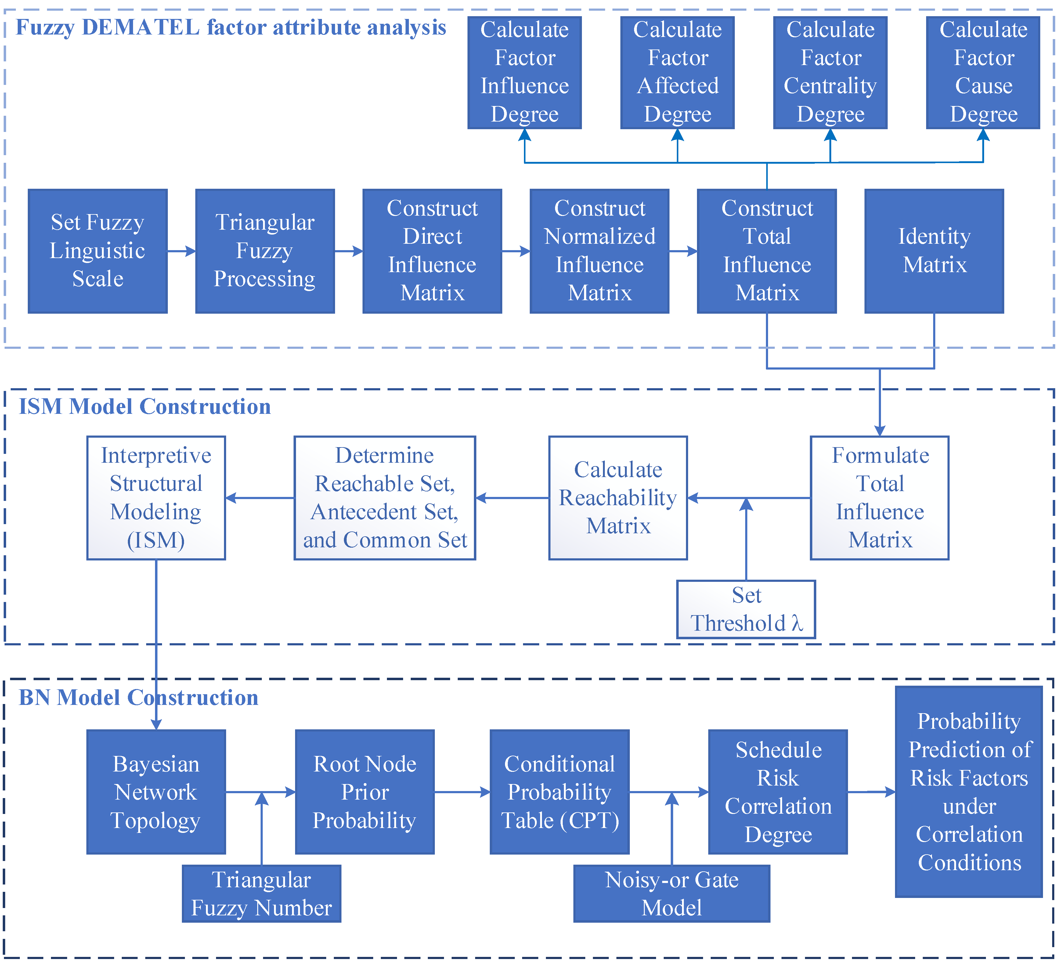
Finally, the hierarchical structure obtained from ISM is mapped onto the topology of a Bayesian network. The prior probabilities of root nodes are determined by aggregating triangular fuzzy numbers derived from expert assessments, while the conditional probabilities of non-root nodes are calculated using the Noisy-OR gate model. By leveraging the probabilistic inference capability of Bayesian networks, the posterior occurrence probabilities of risk factors can be computed under given prior information. Furthermore, the quantitative effects of state changes in individual risk factors on related nodes can be evaluated, enabling dynamic and probabilistic analysis of risk correlation effects. The specific model framework is shown in Figure 1.

2.3.1. Fuzzy DEMATEL Factor Attribute Analysis

Based on the theory of triangular fuzzy numbers, natural language variables are used to provide fuzzy evaluations for each factor, thereby determining their importance and interrelationships. Building on relevant research [22], five levels of influence degree were established. As the score increased, the strength of the influence between factors grew, and conversely, it weakened when the score decreased. The influence of each factor on itself was defined as “NO.” The triangular fuzzy numbers corresponding to each level, along with their descriptions, are presented in

Table 3. Triangular fuzzy number semantic conversion level table.

Fuzzy Level Description	Triangular Fuzzy Number
Very low impact—NO	(0.0, 0.1, 0.3)
Low impact—VL	(0.1, 0.3, 0.5)
Medium impact—L	(0.3, 0.5, 0.7)
High impact—H	(0.5, 0.7, 0.9)
Extremely high impact—VH	(0.7, 0.9, 1.0)

.

A total of n experts are invited to rate the mutual influence of each risk factor at the time of occurrence according to the above five influence degree levels, and then the scoring results are converted into the form of triangular fuzzy numbers in sequence. Let $(l_{ij}^k,m_{ij}^k,r_{ij}^k)$ represent the scoring result of the k-th expert on the influence degree of the i-th factor on the j-th factor in the factor set, where $k\in \left\{k\right|1,2,\dots ,n\}$. The CFCS method is applied to defuzzify the fuzzy numbers of expert scores. The processing steps are shown in Equations (1)–(7).

(1) To accommodate the structural characteristics of triangular fuzzy numbers, the normalization process is defined as shown in Equations (1)–(3).

$$x_{lij}^k={\displaystyle \frac{l_{ij}^k-\min l_{ij}^k}{\max r_{ij}^k-\min l_{ij}^k}}$$

(1)

$$x_{mij}^k={\displaystyle \frac{m_{ij}^k-\min m_{ij}^k}{\max r_{ij}^k-\min l_{ij}^k}}$$

(2)

$$x_{rij}^k={\displaystyle \frac{r_{ij}^k-\min l_{ij}^k}{\max r_{ij}^k-\min l_{ij}^k}}$$

(3)

(2) As shown in Equations (4)–(6), the normalized triangular fuzzy number is transformed into a left standard value ${x^{*}}_{lij}^k$ and a right standard value ${x^{*}}_{rij}^k$, based on which the overall standard value ${x^{*}}_{ij}^k$ is calculated.

$${x^{*}}_{lij}^k={\displaystyle \frac{x_{mij}^k}{1+x_{mij}^k-x_{lij}^k}}$$

(4)

$${x^{*}}_{rij}^k={\displaystyle \frac{x_{rij}^k}{1+x_{rij}^k-x_{mij}^k}}$$

(5)

$$x_{ij}^k={\displaystyle \frac{{x^{*}}_{lij}^k(1-{x^{*}}_{lij}^k)+{x^{*}}_{rij}^k{x^{*}}_{rij}^k}{1-{x^{*}}_{lij}^k+{x^{*}}_{rij}^k}}$$

(6)

(3) Defuzzification. Equation (7) illustrates the calculation and conversion of the k-th expert’s score result on the degree of effect of the i-th factor on the j-th factor to the clear value $b_{ij}^k$:

$$b_{ij}^k=\min l_{ij}^k+x_{ij}^k\times (\max r_{ij}^k-\min l_{ij}^k)$$

(7)

Equation (8) is used to determine the average score of the i-th factor on the j-th factor after all experts’ fuzzy scores on the effect of the i-th factor on the j-th factor are transformed into unambiguous scoring values, as indicated in Equation (8):

$$b_{ij}={\displaystyle \frac{1}{n}}{\displaystyle \sum _{k=1}^n{b}_{ij}^k}$$

(8)

(4) Establishment of a direct influence matrix. According to the influence of horizontal column factors on vertical column factors, Equation (9) illustrates how the direct influence matrix B is created by filling up the matrix with the previously defuzzified impact values between factors.

$$B={\left[b_{ij}\right]}_{n\times n}$$

(9)

(5) Calculation of the normalized influence matrix. The row sum maximum normalization method is used to normalize the matrix B, and the normalization directly affects the matrix G, as shown in Equation (10).

$$G={\displaystyle \frac{1}{\underset{1\le i\le n}{\max }{\displaystyle \sum _j^n}{b}_{ij}}}B$$

(10)

(6) Establishment of a comprehensive impact matrix. The direct and indirect influence relationships between all elements are depicted in the comprehensive influence matrix. The comprehensive influence matrix D can be obtained by continuously multiplying the normalized direct influence matrix G, as shown in Equation (11).

$$D=(G+G^2+\cdots +G^n)={\displaystyle \sum _{n=1}^{\infty }{G}^n}={\displaystyle \frac{G}{I-G}}$$

(11)

where the identity matrix is denoted by I.

(7) Each factor’s impact degree, affectedness degree, centrality, and causality may be computed using the complete influence matrix D. The total effect of a particular factor on all other risk factors in the system is represented by the influence degree e_i; a larger value indicates a stronger ability of the factor to exert influence on the system. The calculation formula is given as follows:

$$e_i={\displaystyle \sum _{j=1}^n{d}_{ij}}\hspace{1em}(i=1,2,\dots ,n)$$

(12)

The affectedness degree f_i. represents the total impact that a given risk factor receives from all other risk factors in the system. A higher value of f_i. indicates that the factor is more susceptible to influences from other factors. The calculation formula is given as follows:

$$f_i={\displaystyle \sum _{i=1}^n{d}_{ij}}\hspace{1em}(i=1,2,\dots ,n)$$

(13)

The degree of the center M_i stands for an individual factor’s total significance inside the complicated system as a whole. It is calculated as the total of its impacted and influence degrees. A higher value of M_i means that the factor has a bigger influence on the system’s overall changes. The following is the expression for the calculation formula:

$$M_i=e_i+f_i$$

(14)

The causality degree N_i reflects the tendency of an individual factor with respect to its influencing role within the system. It is calculated as the difference between the influence degree and the affectedness degree of the factor. A higher value of N_i suggests that the factor is more likely to act as a catalyst for system change. Factor I is categorized as a cause factor when N_i > 0; otherwise, it is recognized as an effect factor. The following is the expression for the calculation formula:

$$N_i=e_i-f_i$$

(15)

The outputs of this section include the centrality and causal attributes of each risk factor, which serve as the basis for defining the risk stratification criteria in the subsequent ISM modeling.

2.3.2. ISM Construction Based on Fuzzy DEMATEL

Although the fuzzy DEMATEL method can quantify the strength of influence and causal attributes among risk factors, its results are primarily presented in matrix form, which makes it difficult to intuitively represent the hierarchical transmission relationships among risks. To further elucidate the hierarchical structure and transmission pathways within the risk system, the ISM method is introduced to structurally reorganize the DEMATEL outputs.

(1) Generate the reachability matrix. Equation (16) addresses a limitation of the fuzzy DEMATEL method—namely, its inability to capture the self-influence of variables—by integrating the comprehensive influence matrix with the identity matrix I to construct the overall influence matrix O. Considering that the influence among certain factors may be relatively weak, a threshold value λ is introduced to optimize matrix O. Using Equation (17), the elements of the matrix are then converted into binary values (0 or 1), thereby yielding the reachability matrix K.

$$O={\left[o_{ij}\right]}_{n\times n}=I+D$$

(16)

$$k_{ij}=\left\{\begin{array}{ll}1,\hfill & o_{ij}\ge \lambda \hfill \\ 0,\hfill & o_{ij}<\lambda \hfill \end{array}\right.$$

(17)

(2) Divide factor hierarchy. The reachability set L(k_i) is the set of factors corresponding to the column with a value of 1 in the i-th row of the reachability matrix K. The antecedent set Q(k_i) is the set of factors corresponding to the row with a value of 1 in the i-th column of the reachability matrix K. First, determine the highest-level factor. h_i is the highest-level factor if there is a factor hi that satisfies Formula (18). Next, simplify the attainable matrix K by eliminating the rows and columns that correspond to h_i from the matrix. Repeatedly perform the above operations until all factors are hierarchized and the final hierarchical structure is constructed.

$$L(h_i)=Q(h_i)\cap L(h_i)$$

(18)

(3) The factor correlation structure is constructed using the reachability matrix, in which the rows and columns correspond to individual risk factors and the matrix elements represent the causal relationships among them. When the element in the i-th row and j-th column equals 1, a directed relationship from factor i to factor j is indicated. Based on the results of factor stratification, directed edges are drawn from lower-level factors to higher-level factors.

To enhance the parsimony and interpretability of the model, transitive reduction is applied to eliminate redundant cross-level transmission paths. Specifically, when indirect transmission paths between two risk factors already exist, the corresponding direct links are removed. This procedure highlights the principal structural relationships within the system and facilitates clearer visualization of the associative connections among risk factors.

The hierarchical risk structure obtained in this section not only reveals the transmission pathways of schedule risks but also provides direct structural evidence for defining node dependencies in the Bayesian network, thereby establishing the topological foundation for subsequent Bayesian network construction.

2.3.3. Prediction of Occurrence Probability of Risk Factors Under Risk Correlation Conditions

The fuzzy DEMATEL-ISM model effectively clarifies the connections and hierarchical structures between factors and constructs a correlation framework. However, the analytical results are limited to the structural level and do not quantify the extent of risk correlation under uncertain conditions. Given the inherent uncertainty and probabilistic characteristics of project schedule risks, this study maps the hierarchical structure derived from ISM into a Bayesian network (BN) topology. Triangular fuzzy numbers and the Noisy-OR gate model are employed to estimate the associated probability parameters. By leveraging the inference capability of the BN, the relationships among risk factors are quantified using probabilistic distributions [23]. This approach enables probabilistic inference of risk interdependencies while preserving the consistency of the underlying causal logic.

(1) Structure mapping

Both the ISM and Bayesian network (BN) models use directed relationships to represent interactions among variables, making their topological structures well suited for integration. In line with the principles of quantifiability, logical rigor, scientific rationality, and systematic completeness, nodes at different hierarchical levels in the ISM are mapped to root, intermediate, and leaf nodes within the BN topology.

(2) Parameter calculation

Once the BN topology is established, the methods used to estimate node parameters directly influence the validity and accuracy of model evaluation. Given the inherent uncertainty and fuzziness of engineering problems, this study adopts a hybrid approach that combines case statistics and expert judgment, integrates fuzzy set theory with the Noisy-OR gate model, and refines the probability estimation process. Consequently, the proposed model enables more scientifically grounded and rational inference and analysis.

(1) Prior probability calculation

Utilizing the concept of triangular fuzzy numbers, in conjunction with expert evaluation results, the grade standard for the root node’s prior probability is defined, with its linguistic value represented by triangular fuzzy numbers. The evaluation levels of “extremely high,” “high,” “medium,” “low,” and “very low” are used to assess the likelihood of each risk factor, with the corresponding triangular fuzzy numbers defined as follows: (0.7, 0.9, 1.0), (0.5, 0.7, 0.9), (0.3, 0.5, 0.7), (0.1, 0.3, 0.5), and (0.0, 0.1, 0.3). Here, $(l_i^k,m_i^k,r_i^k)$ is used to represent the k-th expert’s rating result of the probability of occurrence of the i-th factor in the factor set, where $k\in \left\{k\right|1,2,\dots ,n\}$. In the same way, the CFCS method of Equations (1)–(7) is used to defuzzify the expert rating fuzzy numbers to obtain the prior probability of each root node.

(2) Determination of conditional probability

The Noisy-OR Gate model can solve the conditional probability of non-root nodes with less workload and optimize the calculation process under the condition of determining the Bayesian network topology and expert scoring. The Noisy-OR model assumes that each parent node can independently affect the state change of the child node. Let C be a set of parent nodes. The nodes in the set are independent of each other. Y is the only child node corresponding to the set C. First, it is necessary to determine the probability of the occurrence of a child node in the state of a single parent node, as shown in Equation (19):

$$P_i=(Y\mid {\overline{C}}_1,{\overline{C}}_2,{\overline{C}}_3,\cdots ,C_i,\cdots ,{\overline{C}}_n)$$

(19)

In the formula, C_i represents the occurrence of node events, ${\overline{C}}_i$ represents the non-occurrence of node events, and P_i represents the probability that Y occurs if and only if C_i occurs. The other terms in the conditional probability table of node Y can be determined by using Equation (20):

$$1-P_i={\displaystyle \prod _{C_i\in C}(1-P_i})$$

(20)

When any parent node occurs, the conditional probability of the child node can be calculated according to Equation (21):

$$P(Y)={\displaystyle \sum _{i=1}^n{P}_i}\times P(C_i)\times \overline{P(C_n)}$$

(21)

(3) Calculation of correlation degree

In Bayesian networks, the degree of correlation between nodes can be quantified using the Euclidean distance based on conditional probability distribution information [24]. Specifically, the Euclidean distance is calculated by measuring variations in the posterior probability distributions of child nodes resulting from changes in the state of a parent node, in accordance with the characteristics of the network’s conditional probability structure. The detailed procedure is as follows:

(1) Probability Distribution Extraction: For the target node and its parent, extract the conditional probability distribution of the child nodes in different states of the parent node;

(2) Distance calculation: Calculate the distance value D* according to the Euclidean formula for the probability distribution vector of the child node before and after the parent node state changes, as shown in Equation (22):

$$D^{*}=\sqrt{{\displaystyle \sum _{i=1}^n{(p_i-q_i)}^2}}$$

(22)

In the formula, p_i and q_i represent the probabilities of each state of the child node under two different parent node conditions. A larger Euclidean distance D* indicates that changes in the parent node’s state result in greater perturbations of the child node’s probability distribution, reflecting a stronger correlation between the parent and child nodes.

(4) Occurrence probability prediction

Using the forward inference function, the causal paths from parent to child nodes are followed. By inputting the prior probabilities of root nodes and the conditional probabilities of non-root nodes, the posterior probabilities of the risk factors can be calculated using the Bayesian inference formula. Specifically, this yields the probability P_c of each risk factor resulting from causal propagation.

The probability of risk occurrence obtained through Bayesian network inference is used as a key input parameter for calculating the risk impact coefficient in subsequent buffer zone analysis.

2.4. Buffer Size Calculation

Within the critical chain management framework, buffer sizing is essentially an engineering decision whose rationality depends on how comprehensively sources of schedule uncertainty are characterized. In real-world projects, schedule risks rarely occur independently; instead, interdependencies among risks can lead to cumulative or amplified effects. Therefore, it is necessary to introduce correction mechanisms that capture risk correlation characteristics beyond those addressed by traditional statistical methods.

2.4.1. Process Safety Time

The time of the process was estimated based on the Beta distribution. The crystal ball software was used for simulation to determine the predicted process duration values T_95% and T_50% corresponding to the confidence levels of 95% and 50%, respectively [25,26,27]. Calculate the safety time of Process a:

$$S{T}_a=T_{95\%}-T_{50\%}$$

(23)

The initial buffer bufferl of route l is:

$$buffe{r}_l=\sqrt{{\displaystyle \sum _{a=1}^n{(S{T}_a)}^2}}$$

(24)

2.4.2. Critical Chain Buffer Calculation Under Risk Correlation

In the literature [28], the impact of risk events on activities is determined by both the probability of occurrence and the severity of the events. In risk management, the product of these two factors is referred to as risk exposure. Therefore, this paper employs the DEMATEL model to analyze the attributes, importance, and interrelationships of risk factors affecting project progress and calculates the comprehensive impact M_i of each factor on the entire system. Using the fuzzy DEMATEL-ISM-BN model for the construction period risk correlation structure, the probability P_c of each risk factor resulting from causal transmission is determined. After normalizing M_i, the risk impact coefficient [28] of schedule risk on the entire system is calculated as follows:

$$\vartheta ={\displaystyle \sum _{c=1}^m{M}_c}\cdot P_c$$

(25)

In the formula, M_c is the normalized value of M_i, and $\vartheta$ is the risk impact coefficient of schedule risk on the entire complex system. There are m risk factors that affect the project progress.

The buffer size is calculated by a modified root variance method taking risk correlation into account. The project buffer PB and the import buffer FB are, respectively:

$$PB=\left(1+\vartheta \right)\sqrt{{\displaystyle \sum _{a=1}^n{(S{T}_a)}^2}}$$

(26)

$$FB=\left(1+\vartheta \right)\sqrt{{\displaystyle \sum _{a=1}^n{(S{T}_a)}^2}}$$

(27)

3. Example Analysis

3.1. Project Overview

Using the construction of a pumped storage power station as a case study, the network planning diagram is developed based on a comprehensive analysis of historical data from similar projects and on-site investigations. The project consists of 20 processes, with a planned construction duration of 1998 days. The basic project information is summarized in

Table 4. Basic Information of a Certain Pumped Storage Power Station Construction Project.

Activity Number	Activity Name	Immediate Predecessor Activity	Immediate Successor Activity	Three-Parameter β Distribution
				a	m	b
B	Construction preparation	-	C, D, E, F	170	180	190
D	Ventilation hole	B	G	275	290	305
C	Construction support holes for the tailwater system	B	H	220	235	250
G	Upper Layer Excavation of the Powerhouse	D	I, L	400	415	430
E	Diversion horizontal tunnel construction branch tunnel	B	J	130	145	160
F	Excavation of Upper/Lower Reservoir	B	Q	130	140	150
I	Middle and Lower Layer Excavation of the Powerhouse	G	M	220	235	245
H	Tailrace Tunnel Construction	C	K	280	290	300
M	Powerhouse Floor Slab Concrete Pouring	I	O	23	25	28
J	Diversion horizontal tunnel	E	N	105	110	117
K	Tailwater water filling test	H, L	U	25	28	35
O	Construction of the tail water pipe of the unit	M	R	105	110	120
N	Construction of branch tunnel plugs in the horizontal tunnel of water diversion	J	P	98	105	110
R	Unit volute installation and pressure water test	O	S	100	108	115
P	Water diversion system filling and drainage test	N	U	35	45	55
Q	Filling of Upper/Lower Reservoir	F	U	1135	1150	1165
S	Concrete pouring for unit volute layer, turbine layer, busbar and generator layer	R	T	107	115	120
T	Unit installation	S	U	390	380	400
U	Unit debugging and trial operation	K, T, P, Q	-	130	140	145

, and the progress planning diagram is shown in Figure 2, where L denotes a virtual activity.

The process list, logical relationships, and time parameters presented in Table 4 form the quantitative foundation of this case study. The identification of each process, together with its immediate predecessor and successor relationships, is derived from a comprehensive review of historical construction data from similar pumped storage power stations, the project’s construction organization design documents, and validation by on-site engineering technicians. This ensures that the network structure accurately reflects the typical construction logic and critical path characteristics of this type of project. The duration of each process is estimated using a three-point approach (a, m, b) based on the Beta distribution. These values are derived from the State Grid Xinyuan Group Co., Ltd. (Beijing, China), Science and Technology Project (SGXYTS00GCJS2400157), incorporating research on similar project durations to reasonably represent the uncertainty in process timelines. This table provides the foundational data for subsequent Monte Carlo simulations, critical chain identification, and buffer zone estimation.

3.2. Determine the Critical Route

Based on the established fundamental process information, Figure 2 provides a visual representation of the schedule network plan for this case study. This network serves as the basis for subsequent risk analysis and critical chain identification. By translating the logical relationships among processes defined in Table 4 into a visual network topology, the diagram clarifies the overall project structure and provides the foundation for subsequent Monte Carlo simulations. It establishes both the geometric framework and logical structure required to identify the critical path and calculate process safety margins. Simulation analyses conducted on this network enable the effective mapping of the abstract duration risk factors identified in Section 2 onto specific project elements. Consequently, the results obtained from the risk association model can be directly applied to buffer zone calculations for this project.

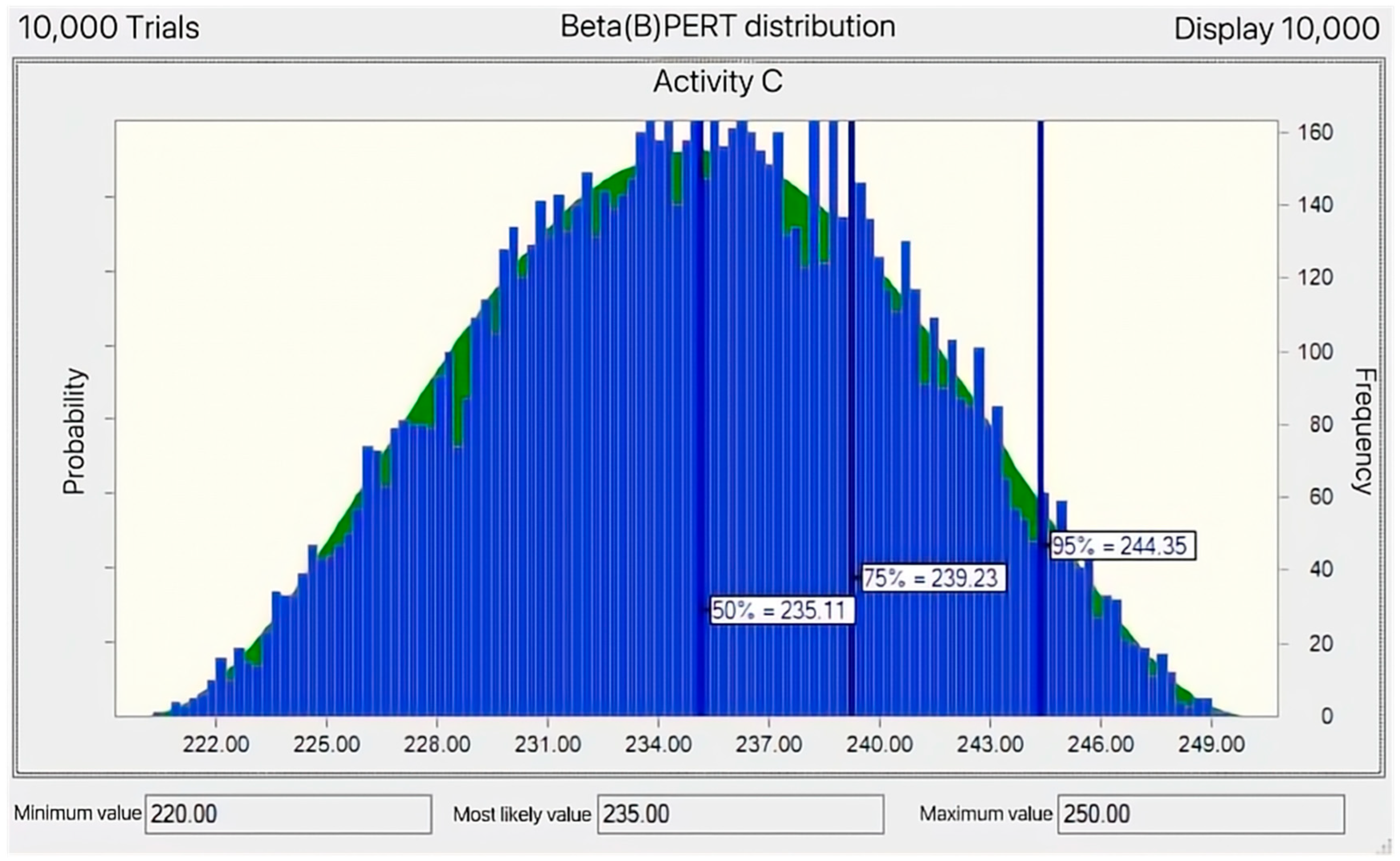
Based on the progress network schedule, the Monte Carlo Crystal Ball software was used to conduct 10,000 Beta(B)PERT distribution simulations for each process of this project. With T_50% as the normal duration of each process and T_95% as the safe completion time, the network progress plan after the simulation is shown in Figure 3. Taking process C as an example, the simulation distribution of process C is shown in Figure 3. For the normal duration of C, T_50% = 235.11 (days) and T_95% = 244.35 (days). According to Equation (23), ST_C = 244.35 − 235.11 = 9.24 (days). The critical route after simulation is B-D-G-I-M-O-R-S-T-U.

3.3. Calculation of Construction Period Risk Correlation Structure Model Based on Fuzzy DEMATEL-ISM-BN

3.3.1. Analysis of Project Progress Risk Factors Based on Fuzzy DEMATEL

Based on the 18 schedule risk factors and corresponding codes defined in the risk factor system for the pumped storage power station project (Section 2.2), a panel of experts was selected for evaluation. All participating experts hold senior technical titles (professor-level senior engineer or associate professor) and have more than ten years of experience in project management, design, or construction of pumped storage power stations or large-scale water conservancy and hydropower projects. Their professional backgrounds cover construction management, engineering design, project supervision, and client-side project management, ensuring a multidimensional and comprehensive understanding of the relevant risk factors. Expert selection was based on field relevance, depth of project experience, and representativeness of professional roles. The assessment adopted a combined approach using structured questionnaires and the Delphi method. In the first round, experts independently conducted fuzzy evaluations according to clearly defined risk factors and the assessment scale shown in Table 3. The research team subsequently compiled the responses and provided anonymized preliminary statistical feedback, enabling experts to discuss areas of divergence. Comparative analysis of expert scores across multiple rounds indicates that the dispersion of indicator scores decreased significantly after the second round, reflecting improved stability and convergence of expert opinions. Although expert judgment is inevitably influenced by individual experience, knowledge structure, and professional background, this study mitigated potential bias by emphasizing professional diversity during expert selection. Moreover, the anonymous, multi-round feedback mechanism of the Delphi method facilitated convergence through systematic comparison of differing viewpoints. As a result, the expert judgment outcomes demonstrate good stability and robustness within the given sample size while preserving opinion diversity.

This study defines the linguistic variables representing levels of influence as follows: no influence (NO), very low influence (VL), low influence (L), high influence (H), and very high influence (VH). Experts were asked to assess the degree of influence between risk factors, resulting in the collection of ten initial scoring matrices. The linguistic variables in these matrices were subsequently transformed into corresponding triangular fuzzy numbers for quantitative analysis.

(1) Construct a comprehensive impact matrix of risk factors during the construction period of pumped storage power stations

Using Equations (1)–(9), MATLAB R2022b software was employed to defuzzify the triangular fuzzy numbers in the ten scoring matrices and to compute the mean influence of each factor on the others, thereby obtaining the direct influence matrix. The row sums of the direct influence matrix were then calculated, and the maximum value was selected as the normalization benchmark. Normalization was performed according to Equation (10) to derive the normalized influence matrix. Subsequently, iterative multiplication was carried out in accordance with Equation (11), yielding the comprehensive influence matrix D, which is presented in

Table 5. Comprehensive impact matrix D.

	X11	X12	X13	X21	X22	X23	X24	X31	X32
X11	0.0841	0.2226	0.2471	0.1062	0.1077	0.1576	0.0761	0.1023	0.1157
X12	0.0692	0.1323	0.1632	0.0663	0.0764	0.0972	0.0628	0.0950	0.0885
X13	0.0822	0.1978	0.1447	0.0721	0.0844	0.1671	0.0684	0.0985	0.0963
X21	0.0775	0.1662	0.2465	0.0760	0.1435	0.2236	0.0917	0.0925	0.0985
X22	0.0676	0.1255	0.1992	0.0658	0.0775	0.1725	0.0689	0.0802	0.0860
X23	0.0726	0.1658	0.2351	0.0699	0.1040	0.1083	0.0695	0.0931	0.0923
X24	0.0811	0.1799	0.2486	0.1385	0.1597	0.2366	0.0763	0.0968	0.1031
X31	0.1251	0.2730	0.2153	0.0876	0.1049	0.1330	0.0822	0.1134	0.1938
X32	0.1201	0.2418	0.2606	0.0999	0.1739	0.2062	0.0949	0.1872	0.1518
X41	0.0693	0.1204	0.1226	0.0655	0.0754	0.0936	0.0621	0.0790	0.0880
X42	0.0771	0.1321	0.1344	0.0671	0.0789	0.0982	0.0635	0.0829	0.1186
X43	0.0841	0.1371	0.1393	0.0656	0.0753	0.0948	0.0618	0.0791	0.0871
X51	0.0741	0.2355	0.1725	0.0719	0.0827	0.1050	0.0681	0.0893	0.0946
X52	0.0697	0.2147	0.1799	0.0675	0.0777	0.0998	0.0640	0.0835	0.0888
X61	0.1063	0.2573	0.2474	0.0980	0.1184	0.1496	0.0928	0.1856	0.2267
X62	0.0997	0.2129	0.2021	0.0916	0.1103	0.1377	0.0867	0.1919	0.2071
X63	0.0671	0.2149	0.1601	0.0647	0.0745	0.0949	0.0613	0.0932	0.0862
X64	0.0901	0.1882	0.1840	0.0843	0.1024	0.1274	0.0799	0.1160	0.2043
	X41	X42	X43	X51	X52	X61	X62	X63	X64
X11	0.0938	0.1547	0.2270	0.0751	0.0785	0.0727	0.0966	0.1556	0.0950
X12	0.0746	0.1122	0.1432	0.0626	0.0655	0.0607	0.0798	0.1986	0.0786
X13	0.0842	0.1425	0.1947	0.0680	0.0710	0.0658	0.0866	0.1488	0.0854
X21	0.0823	0.1192	0.1346	0.0707	0.0739	0.0685	0.0900	0.1338	0.0887
X22	0.0718	0.1035	0.1159	0.0618	0.0646	0.0599	0.0786	0.1135	0.0775
X23	0.0768	0.1116	0.1265	0.0659	0.0689	0.0638	0.0839	0.1777	0.0827
X24	0.0861	0.1245	0.1404	0.0740	0.0774	0.0717	0.0942	0.1405	0.0928
X31	0.1013	0.1820	0.2112	0.0819	0.0856	0.0793	0.1115	0.2750	0.1088
X32	0.1304	0.2690	0.2397	0.0940	0.0982	0.0910	0.2129	0.2238	0.1965
X41	0.0805	0.1697	0.2171	0.0619	0.0647	0.0599	0.0789	0.1076	0.0778
X42	0.1127	0.1133	0.2007	0.0633	0.0661	0.0613	0.0833	0.1187	0.0817
X43	0.1367	0.1467	0.1233	0.0616	0.0644	0.0597	0.0785	0.1091	0.0774
X51	0.0789	0.1132	0.1269	0.0702	0.1478	0.0658	0.0865	0.1895	0.0852
X52	0.0741	0.1068	0.1202	0.0939	0.0690	0.0618	0.0812	0.1447	0.0800
X61	0.1167	0.2404	0.2542	0.0925	0.0967	0.0896	0.1926	0.2810	0.1810
X62	0.1092	0.2428	0.2314	0.0864	0.0903	0.0837	0.1298	0.2189	0.2299
X63	0.0711	0.1026	0.1154	0.0611	0.0639	0.0592	0.0779	0.1168	0.0768
X64	0.1016	0.2440	0.2161	0.0796	0.0832	0.0771	0.2146	0.1530	0.1189

.

The comprehensive impact matrix D shown in Table 5 indicates the strength of mutual influence among the 18 schedule risk factors. This matrix enables preliminary identification of several structural characteristics within the risk system. Firstly, examining the row-wise sum (impact degree e_i), factors X₃₂ (Insufficient owner organization and coordination capability), X₆₁ (Impact of major social events), X₃₁ (Untimely payment of project funds), and X₁₃ (Construction plan changes) exert prominent driving influences across the entire system, acting as pivotal ‘hubs’ triggering risk chain reactions. Secondly, analyzing the column dimension (impact susceptibility f_i), factors X₁₃, X₁₂ (Untimely resource supply), X₆₃ (Interruption of external resource supply), and X₄₃ (Inadequate implementation of work responsibilities and oversight) emerge as highly susceptible ‘vulnerable points’ prone to being affected by other risks. The status of each factor is largely contingent upon changes in other factors within the system. Of particular significance, certain factors—such as X₁₃—exhibit both high influence and high susceptibility. This finding indicates that such factors act not only as critical risk outcomes but also as intermediate nodes in risk propagation, thereby warranting focused attention in risk management. This observation is consistent with the results reported in Reference [17]. Accordingly, the comprehensive influence matrix provides a robust quantitative basis for subsequent calculations of factor centrality and causality, thereby facilitating the clarification of causal attributes and the hierarchical structure of risks.

(2) Calculate centrality and cause degree

Determine the precise impact link between components by calculating the influence degree e_i, affected degree f_i, center degree M_i, and cause degree N_i of each risk factor produced by the fuzzy DEMATEL approach using the complete influence matrix D and combining Formulae (12)–(15). The calculation results are shown in

Table 6. Fuzzy DEMATEL analysis parameter results.

Risk Factor	Influence Degree ei	Affected Degree fi	Center Degree Mi	Center Degree Normalization Mc	Factor Attributes
X11	2.268335978	1.516999587	3.785335565	0.049481693	Causative factor
X12	1.726773506	3.418137671	5.144911177	0.067253989	Outcome factor
X13	1.958575296	3.502644638	5.461219933	0.07138876	Outcome factor
X21	2.077438299	1.458478477	3.535916776	0.046221305	Causative factor
X22	1.69045158	1.827981652	3.518433232	0.045992761	Outcome factor
X23	1.868612324	2.503288098	4.371900422	0.057149236	Outcome factor
X24	2.222153417	1.330865459	3.553018876	0.046444863	Causative factor
X31	2.565092349	1.959824864	4.524917214	0.059149463	Causative factor
X32	3.092057317	2.227592619	5.319649936	0.069538164	Causative factor
X41	1.694077643	1.68267882	3.376756463	0.04414077	Causative factor
X42	1.753838139	2.798851871	4.55269001	0.059512508	Outcome factor
X43	1.68170746	3.138569085	4.820276546	0.063010384	Outcome factor
X51	1.958006854	1.324386576	3.28239343	0.042907262	Causative factor
X52	1.777273391	1.429600688	3.206874079	0.041920077	Causative factor
X61	3.026742772	1.251436212	4.278178984	0.055924115	Causative factor
X62	2.762505917	1.95736113	4.719867047	0.061697836	Causative factor
X63	1.661714572	3.006615387	4.668329959	0.061024146	Outcome factor
X64	2.464501923	1.914545902	4.379047825	0.057242667	Causative factor

.

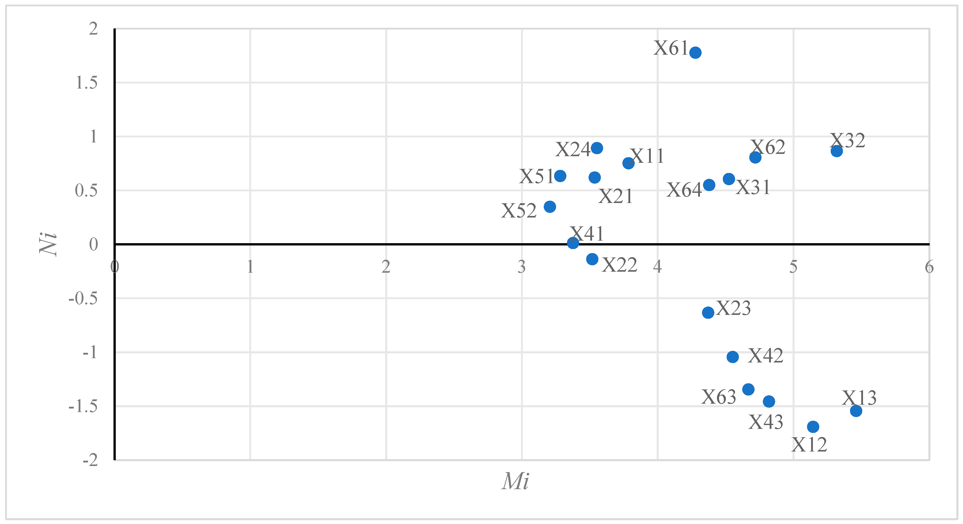
Table 6 presents the influence, affectedness, centrality, and causality of each risk factor calculated using the fuzzy DEMATEL method. The centrality ranking reveals that X₁₃ (Construction plan changes), X₃₂ (Insufficient owner organization and coordination capability), and X₁₂ (Untimely resource supply) occupy the top three positions, indicating that these factors constitute the core hubs influencing the project schedule system. Of particular note, both X₁₃ and X₁₂ exhibit high centrality coupled with negative causality. This corroborates a common phenomenon in engineering practice: frequent alterations to construction plans and delays in supplying critical resources often stem from the cumulative effects of multiple preliminary risks (such as design errors, inadequate coordination, or external events), rather than being isolated initial risk sources. This finding aligns with project management literature asserting that ‘schedule deviations typically manifest as consequences rather than causes’ (Reference [17]). Causality analysis further distinguishes factors into causal and consequential elements. For instance, X₃₂ and X₆₁ (Impact of major social events) exhibit significant positive causality, acting as key independent variables driving systemic risk evolution. This provides quantitative grounds for subsequent ISM stratification and prioritization of risk control measures.

(3) Analyze security risk factor attributes based on fuzzy DEMATEL

The centrality degree represents the overall influence of a factor within the system, with higher values indicating a greater impact on the system as a whole. The causality degree reflects the causal attribute of a factor. Based on the fuzzy DEMATEL results for each risk factor presented in Table 6, a causal relationship diagram of risk factors is constructed, as shown in Figure 4, where the vertical axis represents causality and the horizontal axis represents centrality.

3.3.2. Construction of Security Risk Correlation Structure Based on ISM

(1) Reachable matrix construction based on fuzzy DEMATEL

Based on the comprehensive influence matrix D calculated in Section 3.3.1 and applying Equation (16), the overall influence matrix O is derived. Subsequently, multiple calculations are conducted to select an appropriate threshold λ, using the full impact matrix D’s mean and standard deviation added together to calculate the final threshold λ. Following screening and optimization, the reachability matrix K is obtained, as shown in

Table 7. Reachable matrix K.

	X11	X12	X13	X21	X22	X23	X24	X31	X32	X41	X42	X43	X51	X52	X61	X62	X63	X64
X11	1	1	1	0	0	1	0	0	0	0	1	1	0	0	0	0	1	0
X12	0	1	1	0	0	0	0	0	0	0	0	1	0	0	0	0	1	0
X13	0	1	1	0	0	1	0	0	0	0	1	1	0	0	0	0	1	0
X21	0	1	1	1	1	1	0	0	0	0	0	1	0	0	0	0	1	0
X22	0	1	1	0	1	1	0	0	0	0	0	0	0	0	0	0	0	0
X23	0	1	1	0	0	1	0	0	0	0	0	1	0	0	0	0	1	0
X24	0	1	1	1	1	1	1	0	0	0	1	1	0	0	0	0	1	0
X31	1	1	1	0	0	1	0	1	1	0	1	1	0	0	0	0	1	0
X32	1	1	1	0	1	1	0	1	1	1	1	1	0	0	0	1	1	1
X41	0	0	1	0	0	0	0	0	0	1	1	1	0	0	0	0	0	0
X42	0	1	1	0	0	0	0	0	0	0	1	1	0	0	0	0	0	0
X43	0	1	1	0	0	0	0	0	0	1	1	1	0	0	0	0	0	0
X51	0	1	1	0	0	0	0	0	0	0	0	1	1	1	0	0	1	0
X52	0	1	1	0	0	0	0	0	0	0	0	1	0	1	0	0	1	0
X61	0	1	1	0	0	1	0	1	1	0	1	1	0	0	1	1	1	1
X62	0	1	1	0	0	1	0	1	1	0	1	1	0	0	0	1	1	1
X63	0	1	1	0	0	0	0	0	0	0	0	0	0	0	0	0	1	0
X64	0	1	1	0	0	1	0	0	1	0	1	1	0	0	0	1	1	1

.

Table 7 presents the reachability matrix K obtained by applying the threshold λ. This matrix constitutes a critical transformation step linking the fuzzy DEMATEL analysis with the Interpretive Structural Model (ISM). The distribution of binary entries in the matrix intuitively reveals both direct and indirect influence pathways among risk factors. Moreover, the sparse structure of the matrix reflects the asymmetry and selectivity of risk correlations, indicating that strong associations do not exist among all factors. This finding is consistent with the understanding that risk propagation in practical engineering systems follows specific pathways. By providing clear binary relationship inputs for subsequent hierarchical classification, the matrix ensures logical continuity from numerical assessment to structural modeling within the ISM framework.

(2) Establish a hierarchical structure of schedule risk factors

Based on the hierarchical analysis procedures applied to the reachability matrix K, the schedule risk factors of the pumped storage power station construction project are stratified into different levels. The results of the first-level stratification are presented in

Table 8. ISM first-level division results.

Risk Factor	Reachable Set Li	Antecedent Set Qi	Intersection	Hierarchy
X11	X11, X12, X13, X23, X42, X43, X63	X11, X31, X32	X11	-
X12	X12, X13, X43, X63	X11, X12, X13, X21, X22, X23, X24, X31, X32, X42, X43, X51, X52, X61, X62, X63, X64	X12, X13, X43, X63	The first floor
X13	X11, X12, X13, X23, X42, X43, X63	X11, X12, X13, X21, X22, X23, X24, X31, X32, X41, X42, X43, X51, X52, X61, X62, X63, X64	X11, X12, X13, X23, X42, X43, X63	The first floor
X21	X12, X13, X21, X22, X23, X43, X63	X21, X24	X21	-
X22	X12, X13, X22, X23, X43, X63	X21, X22, X24, X32	X22, X23	-
X23	X12, X13, X23, X43, X63	X11, X13, X21, X22, X23, X24, X31, X32, X61, X62, X64	X13, X23	-
X24	X12, X13, X21, X22, X23, X24, X41, X43, X63	X24	X24	-
X31	X11, X12, X13, X23, X31, X32, X42, X43, X63	X31, X61, X62	X31	The first floor
X32	X11, X12, X13, X22, X23, X31, X32, X41, X42, X43, X62, X63, X64	X31, X32, X61, X62, X64	X31, X32, X62, X64	The first floor
X41	X13, X41, X42, X43	X32, X41, X43	X41, X43	-
X42	X12, X13, X42, X43	X11, X13, X21, X24, X31, X32, X41, X42, X43, X61, X62, X64	X13, X42, X43	-
X43	X12, X13, X41, X42, X43	X11, X12, X13, X21, X23, X24, X61, X62, X41, X42, X43, X51, X52, X61, X62, X64	X12, X13, X41, X42, X43	The first floor
X51	X12, X13, X43, X51, X52, X62	X51	X51	-
X52	X12, X13, X43, X52, X63	X51, X52	X52	-
X61	X12, X13, X23, X31, X32, X42, X43, X61, X62, X63, X64	X61	X61	-
X62	X12, X13, X23, X31, X32, X42, X43, X62, X63, X64	X32, X61, X62, X64	X62, X64	-
X63	X12, X13, X63	X11, X12, X13, X21, X23, X24, X31, X32, X51, X52, X61, X62, X63, X64	X12, X13, X63	The first floor
X64	X12, X13, X23, X32, X42, X43, X62, X63, X64	X32, X61, X62, X64	X32, X62, X64	-

.

Table 8 details the process and outcomes of the first-level classification within the ISM methodology. This iteration identified X₁₂, X₁₃, X₄₃, and X₆₃ as first-level factors, indicating that within the current system architecture, these factors remain unaffected by the remaining factors in the system (i.e., the intersection of their reachable set and antecedent set equals their own reachable set). These factors occupy the most directly observable positions within the hierarchical structure. This process rigorously embodies the core principle of the ISM method—namely, decomposing complex systems into multi-level hierarchical structures—thereby laying a solid foundation for the subsequent construction of multi-level hierarchical models and for understanding the terminal effects of risk propagation.

Table 9. Hierarchical distribution of risk factors.

Hierarchy	Risk Factor
1	X12, X13, X43, X63
2	X22, X23, X42, X52
3	X51, X11, X21, X41, X64
4	X24, X32
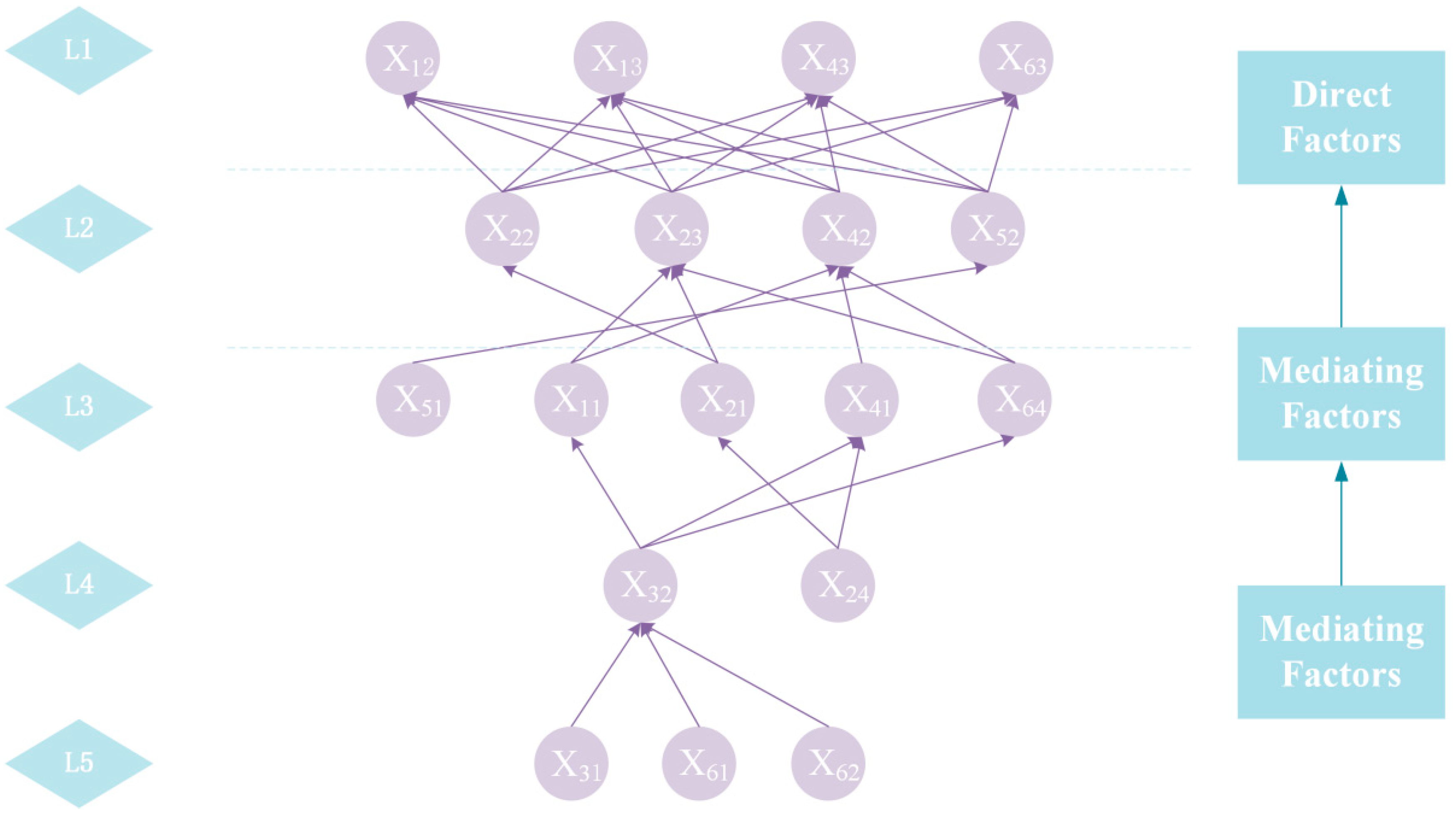
5	X31, X61, X62

summarizes all five risk tiers ultimately derived from the ISM analysis, clearly revealing the multi-layered influence structure among schedule risk factors. From the fifth-tier causal layer (e.g., X₆₁, X₆₂) to the first-tier outcome layer, a complete risk transmission chain is formed. For instance, X₆₁ (major social events) and X₆₂ (land acquisition and resettlement issues) at Level 5, as deep-seated causes, drive risks at Level 4 involving the client and design parties (X₃₂ and X₂₄). These factors subsequently influence lower-level risks associated with construction execution and site supervision, ultimately manifesting at Level 1 as direct schedule delays, such as resource interruptions and design modifications. This multi-tiered structure demonstrates that project delays do not arise from isolated events but result from the sequential transmission and accumulation of risk factors across multiple levels, ranging from external environments and organizational management to on-site execution. This finding deepens the understanding of the systemic complexity of schedule risks in hydraulic engineering projects and provides structured evidence for the development of tiered and prioritized risk response strategies. Specifically, focusing solely on surface-level outcomes is insufficient; effective risk management requires proactive intervention in the underlying driving factors. This perspective is consistent with the principles of systemic risk management.

Based on the hierarchical division results in Table 9, directed connections are established according to the positions of “1” in the reachability matrix K, and transitive simplification eliminates unnecessary cross-level transmission pathways. Lastly, as seen in Figure 5, a risk explanation structure model is built to specify the risk association structure.

Figure 5 visually presents the multi-level hierarchical explanatory structure model for construction schedule risk factors, constructed using the fuzzy DEMATEL-ISM approach. This model clearly parses the inherently complex risk system into five distinct tiers, revealing the complete pathway of risk transmission from deep-seated root causes to surface-level symptoms in a top-down manner. Factors at the fifth tier (X₃₁, X₆₁, X₆₂) constitute the fundamental drivers of the entire risk system, representing ‘deep-seated causes’ requiring strategic or externally coordinated attention. Factors at levels four to two (e.g., X₃₂, X₂₄) serve as ‘intermediate hubs’ for risk transmission and amplification, while first-level factors (e.g., X₁₂ Untimely resource supply, X₁₃ Construction plan changes) represent the ‘direct manifestations’ at the end of the risk chain—‘symptomatic indicators’ requiring immediate monitoring and response during project execution. This structural model not only validates the causal attributes (N_i) identified in the preceding DEMATEL analysis but, more significantly, provides a direct logical framework for constructing the subsequent Bayesian network topology. This ensures a seamless transition from qualitative structural analysis to quantitative probabilistic reasoning. The ultimate significance of this diagram lies in its ability to transform abstract risk “correlations” into concrete, visually explicit, and hierarchically organized “conduction pathways.” In doing so, it provides project managers with a clear and actionable roadmap for implementing systematic risk interventions that target root causes before surface-level symptoms emerge.

3.3.3. Calculation of Construction Period Risk Correlation Degree Based on ISM-BN

(1) ISM mapping to establish the BN structure.

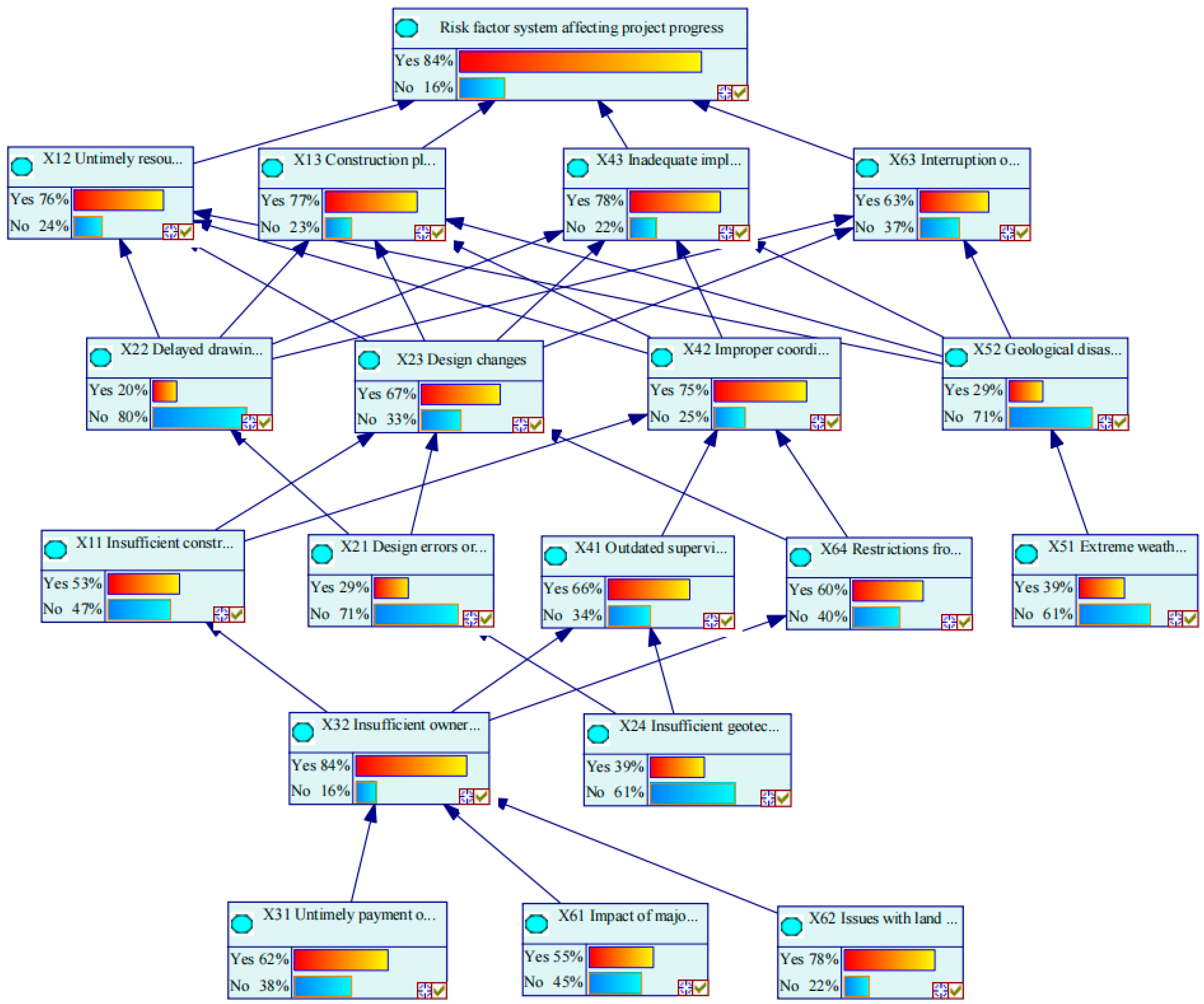
Based on the engineering progress risk correlation structure obtained in Section 3.3.2, the risk interaction network is transformed into a Bayesian Network (BN) topological structure through multi-level hierarchical mapping. Interactions between nodes are defined as one-to-one causal connections, and the overall engineering construction progress risk is represented as a leaf node at the top level of the network. The BN model is constructed and visualized using the Bayesian network software GeNIe 4.0.

This study assumes that the causal structure among risk factors in the Bayesian network can be characterized by the results of the Interpretive Structural Model (ISM) analysis. This assumption ensures logical consistency in the network structure; however, it also implies that the inference results are, to some extent, dependent on the initial structural configuration. If implicit associations or dynamic evolutionary relationships among risk factors are not explicitly identified, they may affect the probabilistic inference outcomes. Consequently, the rationality and validity of the Bayesian network structure play a critical role in determining the reliability of the final analysis results.

(2) Projection of progress risk occurrence probability

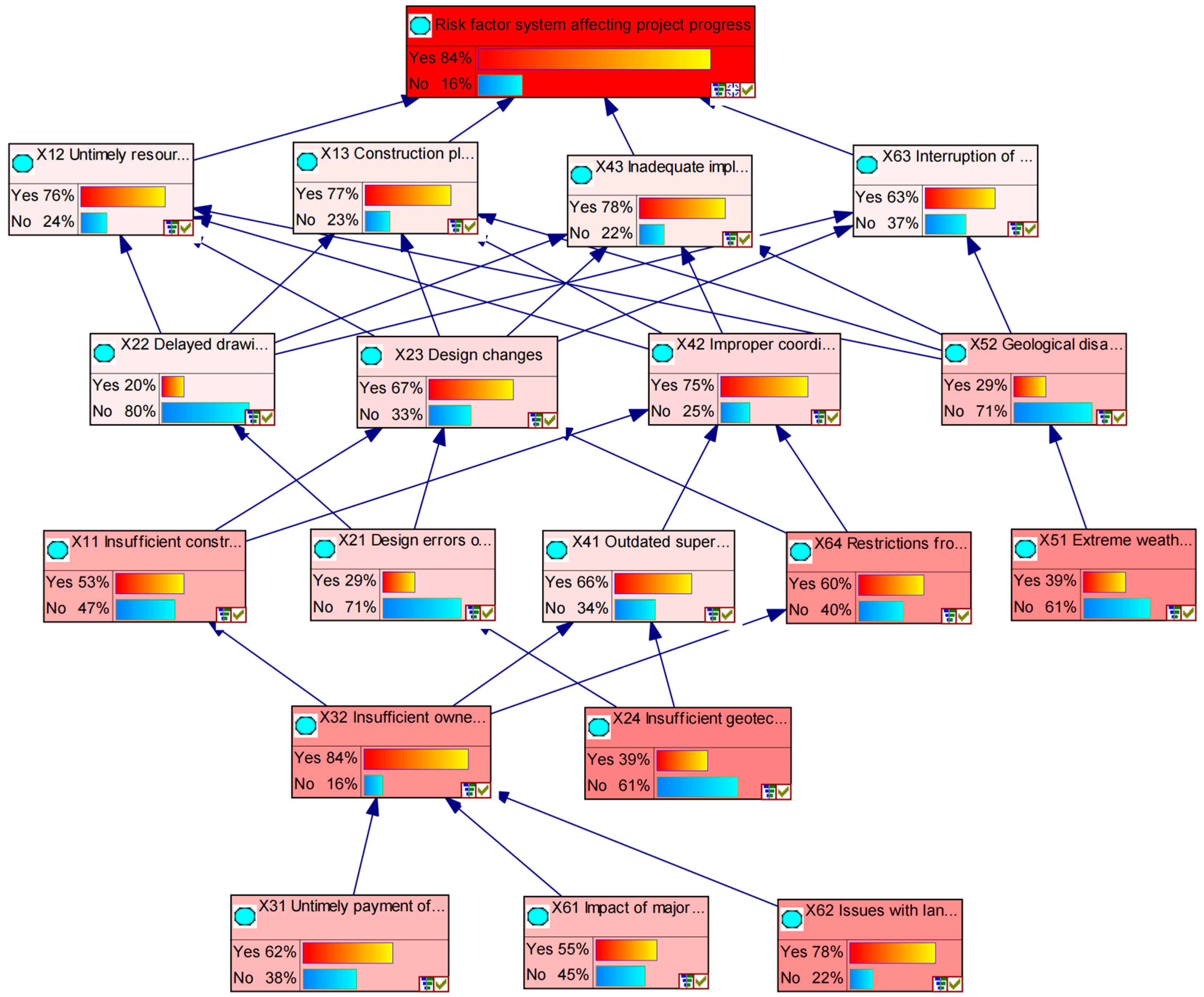
Building on the content discussed in Section 3.3.2, ten experts were invited to assess the occurrence probabilities of the risk factors, integrating construction case data with their extensive professional experience and domain knowledge. Equations (1) and (8) were employed to process the experts’ linguistic assessments by converting them into prior probability levels for the root nodes using the corresponding triangular fuzzy numbers. The prior probability findings for the root nodes X₃₄, X₅₃, X₆₄, X₃₁, X₅₁, X₅₂, and X₆₁ were then computed. The Noisy-OR model is subsequently employed to compute the occurrence probabilities of child nodes under different parent node states, thereby constructing the corresponding conditional probability tables. These probability parameters are then imported into the Bayesian network model in GeNIe for parameter learning. Using forward causal inference, the posterior probability distributions of the 18 risk factors are derived. Finally, the occurrence probability information for each factor is exported and aggregated for subsequent analysis. The reasoning results are presented in Figure 6:

(3) Sensitivity Analysis

The final event construction schedule risk is set to ‘target’, and a sensitivity analysis is conducted on each node within the model. The results are shown in Figure 7.

The color intensity in the diagram visually reflects the sensitivity of each risk factor to its overall impact on the system. Among these, six factors—X₁₁ Insufficient construction experience, X₃₂ Insufficient owner organization and coordination capability, X₂₄ Insufficient geotechnical investigation depth, X₆₄ Restrictions from surrounding residential environment, X₅₁ Extreme weather conditions, and X₆₂ Issues with land acquisition and resident relocation compensation—exhibit the deepest color, indicating the most significant influence on the stability of the project schedule risk system and the likelihood of ultimate schedule delays. These highly sensitive factors play pivotal roles within the system. Specifically, X₆₂, as a causal factor, exerts broad effects on multiple other elements through various pathways. The remaining factors—X₁₁, X₃₂, X₂₄, X₆₄, and X₅₁—act as typical “risk convergence points” or “critical transmission nodes,” being influenced by multiple upstream risks while exhibiting direct and substantial fluctuations in their own states that propagate to the final schedule outcome. The analysis not only validates the reliability of the previously established risk correlation structure model but also provides clear prioritization guidance for project management. From a practical risk control perspective, these highly sensitive factors should be prioritized for continuous monitoring and targeted intervention. Measures such as strengthening client coordination and effectively addressing land acquisition and resettlement issues are expected to yield the greatest improvements in the overall resilience of the project schedule system.

(4) Calculation of risk impact coefficient

Based on the calculation in Table 4, the comprehensive influence degree M_i of individual factors on the entire complex system was calculated and normalized. According to Equation (25), the construction period risk influence coefficient $\vartheta$ was calculated to be 0.566.

3.4. Buffer Size Calculation

3.4.1. Initial Buffer Calculation

The safety time and initial buffer of the process are calculated according to Equations (24)–(26). The calculation results are shown in Table 9.

3.4.2. Project Buffer Size Calculation

It can be calculated from Section 3.3.3 that the impact coefficient $\vartheta$ of the project duration risk is 0.566. According to Equations (25)–(27), when considering the occurrence of the project duration risk correlation, the calculation results of the inflow buffer and project buffer of this project are shown in

Table 10. Buffer size calculation results.

Activity Type	Activity	T95%	T50%	STi	Buffer	FB	PB	Project Total Duration Calculation
Critical Path Activities	B	180.07	186.19	6.12	28.6	-	44.79	2042.79
	D	289.94	299.29	9.35		-
	G	235.11	244.35	9.24		-
	I	414.98	424.35	9.37		-
	M	144.82	154.37	9.55		-
	O	140.01	146.28	6.27		-
	R	234.36	241.6	7.24		-
	S	280.01	296.29	16.28		-
	T	25.11	26.78	1.67		-
	U	110.25	114.2	3.95		-
Non-Critical Path Activities	C	28.5	31.9	3.4	10.08	15.79
	H	110.62	115.66	5.04
	K	104.78	108.18	3.4
	E	107.87	112.32	4.45	14.19	22.22
	J	44.95	51.19	6.24
	N	1149.86	1159.13	9.27
	P	114.62	118.28	3.66
	F	390.02	396.2	6.18	10.36	16.22
	Q	139.4	143.41	4.01

.

The planned construction duration of the project is 1998 days. Considering the interdependencies among risk factors affecting project progress, the critical chain buffer calculated using the improved root variance method proposed in this study is 44.79 days, resulting in a total planned construction duration of 2042.79 days. In contrast, when inter-risk dependencies are ignored, the calculated buffer is only 28.6 days. Although the proposed method leads to a larger buffer size, it more effectively absorbs schedule-related risk impacts and enhances the feasibility and reliability of maintaining the planned project completion time.

3.5. Comparative Analysis

To comprehensively validate the superiority of the proposed method, this section conducts a systematic comparative analysis with existing mainstream approaches across three dimensions: methodological principles, buffer-setting outcomes, and managerial applicability.

First, regarding methodological principles, both the traditional cut-and-paste approach [1] and the root variance method [2] assume risk independence and thus fail to account for inter-factor correlations. Although Monte Carlo simulation [5] can reflect overall uncertainty distributions, it similarly struggles to explicitly characterize causal relationships and dependency structures among risks. In contrast, the integrated fuzzy DEMATEL–ISM–BN model developed herein systematically identifies causal attributes, hierarchical structures, and probabilistic dependencies among risk factors, representing a methodological advancement from “independent risk aggregation” to “correlated risk networks.”

Second, concerning buffer-setting outcomes, as shown in Table 3, Table 4, Table 5, Table 6 and Table 7, the traditional root mean square variance method calculates a project buffer of 28.6 days. By contrast, the present method, while maintaining equivalent process safety time, incorporates the risk correlation effect (ρ = 0.566), increasing the buffer to 44.79 days. This adjustment constitutes a targeted response to potential chain delays arising from risk interdependencies rather than indiscriminate buffer expansion. Compared with the expected duration (2103 days) derived from the triple-time estimation method, the total duration (2042.79 days) obtained using the proposed method remains shorter after a reasonable buffer increase, demonstrating its ability to optimize the trade-off between buffer protection and schedule efficiency.

Finally, with respect to managerial applicability, existing approaches such as Reference [28] primarily rely on a single risk exposure value (RE = 0.45) for monitoring purposes. While higher RE values indicate greater influence on project outcomes and necessitate shorter monitoring cycles, the metric in [28] only considers the occurrence probability of individual risk factors and neglects direct interdependencies between risks. By contrast, the proposed methodology generates risk impact coefficients that more accurately reflect the actual risk network and enables the tracing of critical risk paths through Bayesian networks. This capability facilitates targeted monitoring and contingency planning, particularly enhancing progress risk prevention and control in large-scale water conservancy projects with strong inter-risk dependencies.

In summary, the proposed approach demonstrates substantial improvements over traditional methods across the three dimensions of theoretical modeling, outcome generation, and management support. Consequently, this methodology aligns more closely with engineering practice and provides a robust framework for proactive risk management in complex construction projects.

4. Conclusions

4.1. Research Findings

This study conducts a correlation analysis of construction schedule risk factors in pumped storage power station projects using a hybrid fuzzy DEMATEL–ISM–BN model, systematically identifying the intrinsic relationships and transmission pathways among six major categories of risk factors. By integrating Fuzzy DEMATEL, the Interpretive Structural Model (ISM), and Bayesian Networks (BN), the proposed model not only identifies causal and hierarchical relationships among risk factors but also enables probabilistic reasoning and quantitative analysis of risk propagation. Consequently, it reveals risk accumulation pathways that are difficult to capture under traditional assumptions of independent risks. Regarding critical chain buffer-setting methodology, the traditional root mean square variance approach is enhanced by incorporating a risk impact coefficient derived from the proposed model. This refinement allows buffer sizes to dynamically adjust according to the interrelated structure of the risk system, providing a more scientific and adaptive foundation for schedule control in complex risk environments. Case studies demonstrate that the methodology significantly enhances schedule robustness, improves the predictability of on-time completion, and reasonably increases buffer sizes. Overall, it offers a comprehensive solution for schedule risk management in large-scale, complex engineering projects, combining theoretical innovation with practical applicability.

4.2. Limitations and Future Work

Regarding the applicability of the proposed methodology, this study primarily targets large-scale engineering projects characterized by numerous risk factors, complex interrelationships, and stringent schedule constraints. The core of the analytical framework developed in this study lies in explicitly characterizing the interrelationships among schedule risks and embedding them into the critical chain buffer decision-making process. As a result, the framework exhibits strong potential for broader application in engineering projects that share similar risk characteristics and schedule management requirements. For projects with simpler risk structures or smaller scales, the multi-stage analytical framework may entail redundant implementation efforts and increased analytical complexity. Therefore, in practical applications, the methodology should be appropriately simplified or adjusted according to the project’s complexity and management requirements.

This study integrates systems thinking and probabilistic reasoning into the analysis of engineering schedule risks, moving beyond the traditional reliance on experiential judgments or static risk lists. It provides a novel theoretical framework and empirical evidence to support proactive and refined management of schedule risks in hydraulic engineering projects. Nonetheless, several limitations remain, highlighting potential avenues for future research. This study employs a multi-round anonymous Delphi method to mitigate the subjective influence of expert judgment. Nonetheless, expert evaluations remain inevitably shaped by individual experience, cognitive biases, and prior project backgrounds. Particularly when risk factors are not clearly defined or project information is incomplete, different experts may interpret the same risk differently, thereby affecting the results of subsequent risk correlation analyses. Such effects are primarily reflected in the estimation accuracy of correlation strengths, rather than in fundamental changes to the direction of risk relationships or the overall correlation structure. Consequently, this methodology is most suitable for engineering projects where risk identification is relatively comprehensive and experts demonstrate a high degree of cognitive consistency regarding the research subject. The case validation in this study is based on a single project, and therefore, the generalizability of the findings requires further testing across a broader range of project types and scales. Future research could integrate historical project databases with machine learning techniques to uncover risk correlation patterns, thereby enhancing the objectivity and predictive accuracy of model parameters. In addition, the Bayesian network structure constructed in this study is derived from the hierarchical classification obtained via the ISM. Subsequent studies could explore more flexible structural learning approaches that account for complex, nonlinear interactions among risk factors.

References

1. Goldratt, E.M. Critical Chain; The North River Press: Great Barrington, MA, USA, 1997. [Google Scholar]
2. Newbold, R.C. Project Management in the Fast Lane: Applying the Theory of Constraints; CRC Press: Boca Raton, FL, USA, 1998. [Google Scholar]
3. Herroelen, W.; Leus, R. On the merits and pitfalls of critical chain scheduling. J. Oper. Manag. 2001, 19, 559–577. [Google Scholar] [CrossRef]
4. Herroelen, W.; Leus, R.; Demeulemeester, E. Critical Chain Project Scheduling: Do Not Oversimplify. Proj. Manag. J. 2002, 33, 48–60. [Google Scholar] [CrossRef]
5. Hoel, K.; Taylor, S.G. Quantifying buffers for project schedules. Prod. Inventory Manag. J. 1999, 40, 43–47. [Google Scholar]
6. Kołodziej, K.M.; Łapuńka, I. Determining a Fuzzy Model of Time Buffer Size in Critical Chain Project Management. Eng. Manag. Prod. Serv. 2024, 16, 41–55. [Google Scholar] [CrossRef]
7. Dalouchei, F.; Mousavi, S.M.; Antucheviciene, J.; Minaei, A. A Bi-Objective Model for Scheduling Construction Projects Using Critical Chain Method and Interval-Valued Fuzzy Sets. Buildings 2022, 12, 904. [Google Scholar] [CrossRef]
8. Hongbo, L.; Yiwu, C.; Qiao, L.; Zhu, H. Data-driven project buffer sizing in critical chains. Autom. Constr. 2022, 135. [Google Scholar] [CrossRef]
9. Wu, L.; Zhang, Q. Multi-project management of key chain of carbon fibre and composite materials based on chaos particle swarm optimisation. Int. J. Mater. Prod. Technol. 2023, 67, 281–301. [Google Scholar] [CrossRef]
10. Nie, X.; Li, D.; Li, M.; Guo, Y.; Gao, D.; Sun, Y. Investigation of the Critical Chain Buffer Calculation Model Using Information Entropy and Relay Potential. IEEE Access 2024, 12, 157455–157465. [Google Scholar] [CrossRef]
11. Nie, X.; Li, M.; Lu, J.; Wang, B. Research on Buffer Calculation Model of Critical Chain Based on Adjacency Information Entropy. Buildings 2023, 13, 942. [Google Scholar] [CrossRef]
12. Nie, X.; Ling, L.; Su, B.; Wang, B. Research on Key Chain Buffer Calculation Method Considering Multi-objective Multi-Resource Constraints and Relay Potential. Water Power 2021, 47, 106–110. [Google Scholar]
13. Zhang, J.; Ji, F. Project Buffer Management Based on Activity Resilience. Chin. J. Manag. 2020, 17, 924–930. [Google Scholar]
14. Zhang, J.; Lyu, Y. Determination of Critical Chain Project Buffer Monitoring Cycle Based on Objective and Activity Risk. Oper. Res. Manag. Sci. 2024, 33, 86–92. [Google Scholar]
15. Huang, J.; Wang, Y.; Wang, Y.; Gong, S.; Zhang, Y.; Ye, L. Critical chain buffer zone setting in project schedule management from resource flexibility perspective. Yangtze River 2022, 53, 149–154. [Google Scholar]
16. Zhang, J.; Cheng, N. Determination of Critical Chain Project Monitoring Interval Based on Risk-Driven. Ind. Eng. Manag. 2021, 26, 10–17. [Google Scholar]
17. Bai, L.; Zhang, L.; Sun, Y.; Yang, Q.; Qin, X. Prevention Strategy of Highway Project Portfolio Construction Schedule Risk. China J. Highw. Transp. 2021, 34, 203–214. [Google Scholar]
18. Liu, J. Correlation analysis of scheduling risks based on BN-CPM. J. Hydroelectr. Eng. 2011, 30, 199–203. [Google Scholar]
19. Huang, J.; Tan, Y.; Chen, M.; Wang, X.; Jiang, H.; Jiang, Y. Research on Risk Transfer Route of Underground Cavern Group Construction Schedule Based on ISM-SD. Water Resour. Power 2024, 42, 93–97. [Google Scholar]
20. Huang, Y.; Zhang, L.; Wang, K. Metro Station Project Schedule Management Based on Link and Proiect Characteristics. Chin. J. Undergr. Space Eng. 2021, 17, 334–342. [Google Scholar]
21. Li, X.; Tian, J.; Zheng, J.; Su, Z. Risk analysis on construction progress of water conservancy project. Water Resour. Hydropower Eng. 2018, 49, 141–147. [Google Scholar]
22. Liu, R.; Zhang, J.; Han, X. Risk identifiation based on triangular fuzzy number for construction project. J. Harbin Inst. Technol. 2008, 10, 1617–1620. [Google Scholar]
23. Zhang, Y.; Wang, X. Study on causes of unsafe behaviors of construction workers based on DEMAREL-ISM-BN. J. Saf. Sci. Technol. 2020, 16, 110–116. [Google Scholar]
24. Wang, Q.; Jing, H.; Guo, Z.; Wang, Z. Risk early warning model of technological innovation achievements transformation in major construction proiects based on DEMATEL-ISM-BN. J. Railw. Sci. Eng. 2025, 22, 1315–1327. [Google Scholar]
25. Ni, T.; Chang, H.; Song, T.; Xu, Q.; Huang, Z.; Liang, H. Non-intrusive Online Distributed Pulse Shrinking Based Interconnect Testing in 2.5D IC. IEEE Trans. Circuits Syst. II Express Briefs 2020, 67, 2657–2661. [Google Scholar] [CrossRef]
26. Ni, T.; Yao, Y.; Chang, H.; Lu, L.; Liang, H.; Yan, A. LCHR-TSV: Novel Low Cost and Highly Repairable Honeycomb-Based TSV Redundancy Architecture for Clustered Faults. IEEE Trans. Comput.-Aided Des. Integr. Circuits Syst. 2019, 10, 2938–2951. [Google Scholar] [CrossRef]
27. Hu, X.; Ma, P.; Gao, B.; Zhang, M. An Integrated Step-Up Inverter Without Transformer and Leakage Current for Grid-Connected Photovoltaic System. IEEE Trans. Power Electron. 2019, 34, 9814–9827. [Google Scholar] [CrossRef]
28. Zhang, J.; Zhou, S. Buffer Sizing of Critical Chain Projects Based on Uncertainty. J. Ind. Technol. Econ. 2021, 40, 154–160. [Google Scholar]
Figure 1. Fuzzy DEMATEL-ISM-BN-Based Risk Correlation Structure Model Framework Diagram.
Buildings 16 00557 g001
Figure 2. Schedule diagram of a certain pumped storage power station construction project.
Buildings 16 00557 g002
Figure 3. Simulation distribution diagram of process C.
Buildings 16 00557 g003
Figure 4. Risk factor causal relationship diagram.
Buildings 16 00557 g004
Figure 5. Framework diagram of risk correlation structure model based on fuzzy DEMATEL-ISM-BN.
Buildings 16 00557 g005
Figure 6. Forward reasoning of project schedule risks of pumped storage power station.
Buildings 16 00557 g006
Figure 7. Risk Sensitivity Analysis of Construction Progress for Pumped Storage Power Station Projects.
Buildings 16 00557 g007