Article

A TSception–Transformer–TCN-Based Temperature-Prediction Method for Enclosed Cold-Aisle Data-Center Rooms

1
School of Mechanical and Automotive Engineering, South China University of Technology, No. 381, Wushan Road, Tianhe District, Guangzhou 510640, China
2
Guangzhou Institute of Modern Industrial Technology, South China University of Technology, Guangzhou 510640, China
3
Guangdong Artificial Intelligence and Digital Economy Laboratory (Guangzhou), Pazhou Lab, Guangzhou 510330, China
*
Author to whom correspondence should be addressed.
Buildings 2026, 16(18), 3580; https://doi.org/10.3390/buildings16183580
Submission received: 1 July 2026 / Revised: 26 August 2026 / Accepted: 7 September 2026 / Published: 9 September 2026

Abstract

In enclosed cold-aisle data-center rooms, hotspot temperatures within the cold aisles are directly related to server inlet air safety and air-conditioning operation performance. Therefore, high-accuracy temperature prediction is of great significance for thermal-risk warning and operational optimization. This study focuses on an enclosed cold-aisle data-center room in a large data center located in a hot-summer and warm-winter region. The maximum temperature of one selected cold aisle is taken as the prediction target, and a hybrid prediction model integrating TSception, Transformer, and TCN is proposed to characterize multi-scale local disturbances and cross-period temporal dependencies. The model inputs and historical time window are determined through cold–hot separation analysis, cold-aisle temperature-stability comparison, lag analysis between supply air temperature and cold-aisle temperature, and correlation analysis of candidate variables. The experimental results show that the proposed model achieves an MAE of 0.285 °C, an RMSE of 0.438 °C, an NRMSE of 4.76%, and a MAPE of 1.13% in predicting the cold-aisle temperature of the AB aisle, outperforming Persistence, BP, LSTM, XGBoost, and several ablation models. Further multi-aisle experiments demonstrate that the proposed model consistently maintained low prediction errors in independent prediction tasks across different cold aisles, indicating good applicability of the model architecture for characterizing temperature time series in multiple cold aisles within the same data-center room. The proposed method can provide a reference for hotspot-risk identification in enclosed cold aisles and operational optimization of precision air-conditioning systems.

1. Introduction

1.1. Background

Data-center cooling systems are responsible for maintaining a stable thermal environment and ensuring reliable operation of IT equipment. Among common airflow-management strategies, cold-aisle containment offers clear advantages in reducing mixing between hot and cold airstreams and improving cooling-capacity utilization [1]. In practical operation, however, the thermal environment in a data-center room is still affected by IT-load fluctuations, supply air regulation, local airflow-distribution differences, and spatial heat-storage effects. As a result, the cold-aisle temperature field is often non-uniform, and local hotspots may still occur [2]. When the IT load rises abruptly, airflow distribution becomes imbalanced, or the response of the precision air-conditioning units lags behind the thermal disturbance, local cold-aisle temperatures may approach or exceed the safety limit within a short period. Conventional control strategies based primarily on return-air temperature feedback cannot promptly reflect multi-point temperature changes, which may delay thermal-risk identification and lead to insufficient cooling adjustment [3]. Therefore, cold-aisle temperature prediction is necessary not only for improving thermal-environment perception but also for ensuring room-level thermal safety and enabling anticipatory regulation and optimized control of precision air-conditioning systems.
Existing studies on data-center temperature prediction mainly focus on estimating the overall room temperature field or predicting temperatures at representative monitoring points [4,5]. Research specifically addressing local hotspot temperature in enclosed cold aisles remains limited. On the one hand, cold-aisle temperature does not evolve synchronously on a single timescale. Short-term disturbances, control responses, and heat accumulation are superimposed, so the sequence contains both rapid fluctuations and persistent evolution. On the other hand, control variables such as supply air temperature, the number of operating air-conditioning units, and airflow speed often affect the target temperature with a time lag. The temperature-evolution process cannot be fully represented using information from a single time step. If the model cannot simultaneously account for local multi-scale feature extraction, cross-temporal dependency modeling within the historical window, and downstream temporal feature integration, its ability to characterize the dynamic variations in cold-aisle temperature will be limited.
Based on the above considerations, this study takes an enclosed cold-aisle room in a large data center as the research object and investigates the prediction of the maximum temperature in one cold aisle. Input samples for the prediction task are constructed through thermal-environment characterization, lag-correlation analysis, and feature screening. In terms of model design, a hybrid structure integrating TSception, Transformer, and TCN (temporal convolutional networks) is proposed to improve the representation of complex dynamic features in temperature sequences of enclosed cold-aisle data-center rooms. Finally, comparative experiments and ablation experiments are conducted to verify the effectiveness of the proposed method.

1.2. Related Works

Hotspot temperature prediction in enclosed cold-aisle data-center rooms is an important basis for thermal-risk warning and optimized control of precision air-conditioning systems. Existing temperature-prediction methods for data-center rooms can be broadly divided into physics-based simulation methods and data-driven methods based on historical operational data. Physics-based methods, represented by computational fluid dynamics (CFD), can solve the conservation equations of mass, momentum, and energy to describe airflow organization, heat transfer, and local hotspot distribution in detail. They are valuable for room design, airflow-organization optimization, and cooling-scheme evaluation [6]. Guo et al. [7] proposed a coupled CFD and flow-network modeling framework that improved computational efficiency while considering both overall airflow patterns and local temperature-field prediction. Singh et al. [8] used CFD to analyze differences in the thermal environment before and after cold-aisle containment retrofitting, verifying the effectiveness of aisle containment in improving cold-air utilization. Szeliga et al. [9] developed an automated simulation framework, CFD4DC, and achieved good prediction accuracy in thermal analysis of a micro data center. Nevertheless, CFD strongly depends on geometric modeling, mesh generation, and boundary-condition specification. Its high computational cost and long simulation time make it more suitable for offline analysis and scheme comparison than for real-time online prediction and control [10].
To improve prediction efficiency, data-driven methods have gradually become an important direction in data-center temperature prediction. Traditional machine-learning methods, such as support vector regression, Gaussian process regression, random forest, XGBoost, and LightGBM, can establish mappings between operational variables and target temperatures based on historical monitoring data. These methods are attractive because of their relatively simple modeling procedures and fast inference speed. Xu et al. [11] developed an ensemble-learning framework combining support vector regression, linear regression, and LightGBM for temperature prediction, and the results showed that the ensemble outperformed individual models. Patel and Joshi [12] compared Gaussian process regression, artificial neural networks, and support vector regression for static temperature prediction and found that Gaussian process regression achieved good accuracy under small-sample conditions. Deng et al. [13] generated samples using CFD simulations and compared random forest (RF), eXtreme Gradient Boosting (XGBoost), and stacked ensemble models for data-center temperature-field prediction. Lin et al. [14] further pointed out that, in multi-output and multi-step prediction scenarios, the training and inference costs of SVR and GPR increase significantly as the data scale grows, and their overall performance is weaker than that of XGBoost and LightGBM. However, these methods usually rely on manually designed features and provide insufficient characterization of temporal correlation, non-stationary fluctuations, and multivariable coupling commonly found in data-center thermal environments. Their prediction performance is therefore constrained under dynamic operating conditions with frequent load variations and air-conditioning adjustments.
Deep-learning methods can automatically extract high-level features from multivariate time series and have been applied to the prediction of server inlet temperature, cold-aisle temperature, and room-level thermal-environment indicators. Asgari et al. [15] combined CFD with ANN to construct a gray-box model that balances physical interpretability and computational efficiency. Sahar et al. [16] integrated physical equations with ANN and achieved rapid real-time temperature prediction. Lloyd and Rebow [17] used measured data from multiple data centers and combined clustering with ANN to develop a data-driven model for predicting rack-temperature distributions at multiple heights. Wang et al. [18] used LSTM (Long Short-Term Memory) to predict server inlet temperature and improved model generalization and stability through hyperparameter optimization. Zhang et al. [19] proposed a dual-channel residual Re-LSTM network and enhanced its adaptability to missing-data scenarios by introducing shortcut connections of key thermodynamic parameters. Graph neural networks have also been used to introduce rack-layout or sensor-topology relationships and thereby enhance spatial-correlation representation [20]. Recurrent neural networks and their variants can model temporal dependencies, but they have limited training efficiency for long sequences and limited capability to capture long-term dependencies [21]. Convolutional structures are suitable for extracting local patterns, yet they are not sufficient for characterizing long-range temporal correlations [22]. Transformer models have advantages in global dependency modeling due to the self-attention mechanism, but their ability to directly capture local abrupt changes and multi-scale dynamic features remains insufficient [23]. For enclosed cold-aisle data-center rooms, hotspot temperature is jointly affected by IT-load disturbances, supply air regulation, airflow organization, and spatial heat storage. The resulting temperature sequence often contains short-term fluctuations, cross-period lag effects, and slow evolution simultaneously, making it difficult for a single model structure to fully represent the complex dynamic process.
In recent years, multi-scale convolution, attention mechanisms, and temporal convolutional networks have demonstrated complementary strengths in time-series forecasting. Multi-scale convolution is beneficial for extracting local variation features at different temporal scales [24], attention mechanisms enhance cross-period dependency representation [25], and temporal convolutional networks further extract and integrate local temporal features, thereby enhancing the model’s ability to represent dynamic information within the sequence [26]. Although previous studies have demonstrated the effectiveness of these structures in general time-series forecasting, the alignment between model architecture and actual thermal-response characteristics remains insufficient for temperature prediction in enclosed cold-aisle data-center rooms. Therefore, this study combines deep temporal modeling with the thermal-environment characteristics of enclosed cold-aisle rooms and develops a hybrid prediction model integrating TSception, Transformer, and TCN to improve the representation of multi-scale dynamic variations in the maximum cold-aisle temperature.

2. Materials and Methods

In an enclosed cold-aisle data-center room, cold-aisle temperature variations are jointly caused by IT-load fluctuations, air-conditioning regulation, changes in airflow organization, and heat accumulation. Server-load variations and local mixing of hot and cold airstreams can cause temperature fluctuations at a short timescale. Adjustments to supply air temperature, airflow speed, and the number of operating air-conditioning units produce responses at an intermediate timescale. Continuous heat dissipation from racks and heat accumulation within aisles further lead to slow temperature evolution. Accordingly, cold-aisle temperature sequences exhibit local disturbances, multi-timescale responses, and long-term dependencies, requiring prediction models to effectively capture local variations and cross-temporal dependencies while integrating temporal features.
To represent these thermal-environment features, the model adopts a hybrid structure composed of TSception, Transformer, and TCN. TSception is used to extract multi-scale local features [27], while the Transformer captures cross-temporal dependencies among historical states. TCN further integrates local dynamic features through temporal convolution and residual connections, thereby enhancing the propagation of temporal information [28]. Their sequential combination enables the model to represent short-term disturbances, medium-term responses, and slow temperature-evolution patterns simultaneously.

2.1. TSception-Based Multi-Scale Temporal Feature Extraction

Cold-aisle temperature is jointly influenced by multiple factors, including IT load, air-conditioning operating conditions, and historical thermal inertia, resulting in dynamic variations across different timescales. To extract local variation information over different historical time ranges, this study introduces depthwise separable convolution to construct a parallel temporal feature-extraction module following the multi-scale temporal convolution concept of TSception. The module first extracts the local dynamic features of each input variable along the temporal dimension and then performs information fusion across different feature channels through pointwise convolution. The basic structure of the module is shown in Figure 1.
Let the input sequence be X ∈ T × C , where T is the number of time steps and C is the number of feature channels. TSception first uses depthwise separable convolution to reduce computational cost. This operation consists of depthwise convolution and pointwise convolution:
(1)
Depthwise convolution, performed independently for each channel:
Z d = DepthwiseConv ( X ) = c = 1 C X : , c K c
where Σ denotes channel concatenation, X:,c is the input sequence of the c-th channel, Kc k d is the convolution kernel for that channel, and kd is the depthwise convolution kernel size.
(2)
Pointwise convolution for cross-channel information fusion:
Z p = PointwiseConv ( Z d ) = Z d W p + b p
where Wp C × C is the 1 × 1 convolution weight matrix, bp is the bias term, and C is the number of output channels.
Subsequently, three parallel branches perform temporal convolution using kernels of different sizes to capture short-, medium-, and long-term patterns, respectively. Each branch is configured with 64 output channels, a stride of 1, and a dilation rate of 1, while same padding is applied to preserve the temporal dimension. With a sampling interval of 15 min, kernel sizes of 3, 5, and 7 time steps correspond to historical information spans of approximately 45, 75, and 105 min, respectively, thereby generating local dynamic feature representations at different temporal scales.
F i = ReLU Conv 1 D ( Z p , k i ) + b i , k i { 3 , 5 , 7 }
The outputs of the three branches are finally concatenated along the feature dimension:
F multi = Concat ( F 1 , F 2 , F 3 ) T × ( 3 C )
This module captures local variation features of temperature sequences under different receptive fields and provides multi-scale feature representations for subsequent global modeling.

2.2. Transformer-Based Global Temporal Dependency Modeling

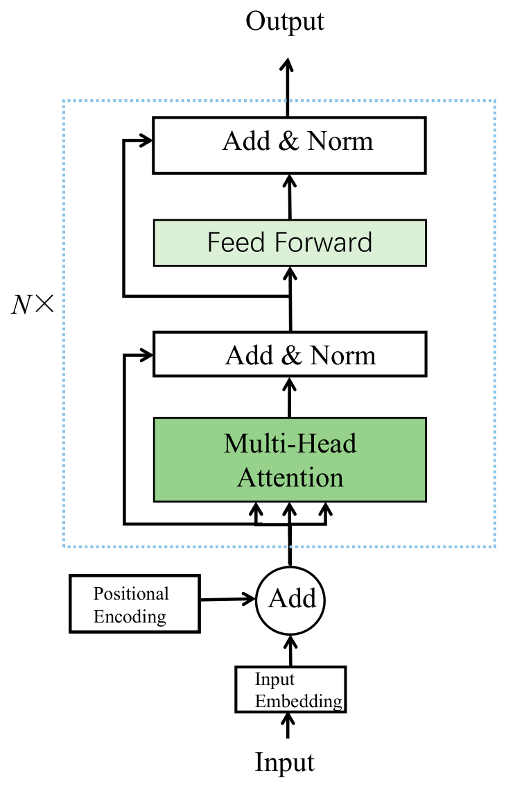
Multi-scale temporal convolution can extract local dynamic features over different receptive fields; however, feature interactions are mainly constrained by the convolutional receptive field. To further capture the relationships among operating states at different time steps within the historical window, a Transformer encoder module is introduced to perform global modeling of the multi-scale temporal features. Its structure is shown in Figure 2.
The Transformer is based on the self-attention mechanism, which captures global dependencies by calculating correlations between any two temporal positions in a sequence. The core computation is as follows:
Attention ( Q , K , V ) = softmax Q K T d k V
where Q, K, and V are the query, key, and value matrices, respectively, and d k is the scaling factor.
The self-attention mechanism adaptively weights the features at different time steps by computing the correlations among different temporal positions within the historical window, thereby extracting cross-temporal state-dependency information. To enhance the representation of temporal information in different feature subspaces, a multi-head self-attention mechanism is adopted. The outputs of multiple attention heads are concatenated and then linearly projected:
MHA ( Q , K , V ) = Concat ( head 1 , head 2 , , head h ) W O
head i = Attention ( Q W i Q , K W i K , V W i V )
where headi denotes the output of the i-th attention head; h is the number of attention heads; WiQ, WiK, and WiV denote the query, key, and value projection matrices corresponding to the i-th attention head, respectively; and WO is the output projection matrix of the multi-head attention mechanism.
Considering that the output of the TSception module contains 192-dimensional fused features at multiple temporal scales, multi-head attention is employed to learn the relationships among different time steps within the historical window from different feature subspaces. In this study, eight attention heads are used, allowing different heads to focus on different types of temporal dependencies without incurring the additional model parameters and computational complexity associated with a larger number of attention heads. After Transformer encoding, the feature dimension remains unchanged, and the resulting features are used as the input to the subsequent temporal convolution module.
This module establishes dependencies among different sampling time steps within the given historical window and complements the local dynamic features extracted by the preceding multi-scale convolution module. It therefore provides a temporal feature representation containing both local variations and cross-temporal dependencies for subsequent temperature prediction.

2.3. TCN-Based Temporal Convolutional Feature Integration

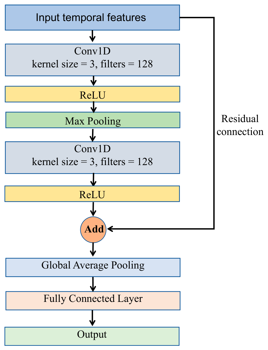
The Transformer module establishes state dependencies among different time steps within the historical window. To further extract local temporal variations and enhance feature propagation, a one-dimensional temporal convolution module with residual connections is employed to integrate the Transformer output. Its architecture is shown in Figure 3.
Let the output features of the Transformer be HTr. For the l-th residual block, the convolutional transformation can be expressed as follows:
F ( H l ) = σ Conv 1 D ( H l ; W l , b l )
The output of the residual block is given by the following:
H l + 1 = F ( H l ) + P ( H l )
where F(·) denotes the convolutional feature transformation, σ(·) represents the ReLU activation function, and P(·) denotes the residual branch.
When the input and output feature dimensions are identical, P(·) adopts an identity mapping; when the feature dimensions differ, a 1 × 1 convolution is used for dimensional matching. The residual connection preserves the input features and facilitates gradient propagation in deep networks, thereby effectively retaining the historical-state information encoded by the Transformer during subsequent local temporal feature extraction.
In this study, the temporal convolutional layer uses a kernel size of 3, 128 filters, and the ReLU activation function. After residual fusion, max pooling is applied to compress the temporal dimension, followed by subsequent convolutional layers to further extract local dynamic features. Finally, global average pooling is used to obtain a fixed-length feature vector, which is passed through a fully connected layer to predict the maximum cold-aisle temperature at the next sampling time step.
For the eight-step historical input used in this study, the model predicts the target at time, t, using only the operating information from t − 8, …, t − 1, without introducing observations from the target time step or any future time steps.

2.4. Analysis of the Model Structure

From the perspective of the overall architecture, the proposed model consists of three sequential stages: multi-scale temporal feature extraction, global dependency modeling, and temporal feature integration. The front-end TSception module employs depthwise separable convolutions with different kernel sizes in parallel to extract multi-scale local dynamic features from the historical sequence, while pointwise convolution is used to fuse information across different input variables. The Transformer encoder module further establishes dependencies among different time steps within the historical window, thereby enhancing the interaction of cross-temporal state information. The TCN module then integrates local dynamic features through temporal convolution and residual connections while preserving information from the preceding layers. These three modules sequentially perform multi-scale local feature extraction, cross-temporal dependency modeling, and temporal feature integration, thereby forming a unified temporal modeling framework for short-term prediction of the maximum cold-aisle temperature.

3. Case Study

3.1. Study Object and Data Source

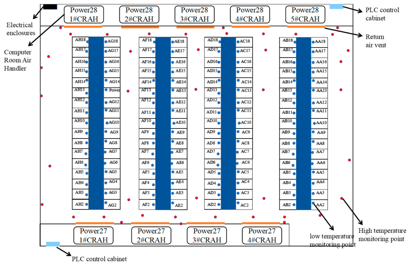
The research object is an enclosed cold-aisle room in a large data center located in a hot-summer and warm-winter region, as shown in Figure 4. The room is supplied with cooling by precision air-conditioning units (Guangdong Shenling Environmental Systems Co., Ltd., Foshan, China), and the enclosed cold-aisle structure is used to strengthen the separation between hot and cold airstreams. The data-center room has a total floor area of 292.5 m2 and contains eight rows of server racks and 170 temperature monitoring points. Among them, 136 monitoring points are located in the cold aisles and 34 in the hot aisles. These sensors (Guangzhou i-MEC Technology Co., Ltd., Guangzhou, China) are positioned in the central regions of the aisles on the air-inlet and air-exhaust sides of the racks, respectively, at a height of approximately 1.5 m above the floor. The temperature measurement range is −10 to 60 °C, with a measurement error within ±0.5 °C, enabling the monitoring system to provide a relatively comprehensive representation of the spatial temperature distribution within the data-center room. The airflow organization uses underfloor supply through perforated floor tiles and side return air. Cold air is delivered into the cold aisles through the floor, enters the racks, absorbs heat generated by IT equipment, and then returns to the precision air-conditioning units through the hot aisles.
The cold aisle is located on the air intake side of the server racks, and its air temperature can characterize the local thermal environment in the server inlet region. Since the actual server inlet temperature is also affected by internal rack airflow organization, equipment layout, and local airflow rate, certain differences may exist between the cold-aisle temperature and the inlet temperature of an individual server. In this study, the maximum temperature among the monitoring points in the cold aisle is used as a characteristic indicator of the local thermal environment to represent the relatively unfavorable thermal condition on the rack inlet side and is taken as the target variable for subsequent short-term temperature prediction.
This study uses actual operating data recorded by the data-center monitoring system from 00:00 on 1 June 2025 to 09:00 on 1 August 2025, with a sampling interval of 15 min. The monitored variables include IT equipment load power, hot aisle temperature, cold-aisle temperature, supply and return air temperatures of the precision air-conditioning system, the number of operating precision air-conditioning units, and the fan-speed ratio. After data preprocessing, a total of 5880 valid operating samples were obtained. Considering the temporal characteristics of the prediction task, the data were first divided chronologically into training, validation, and test sets without random shuffling, with proportions of 70%, 10%, and 20%, corresponding to 4116, 588, and 1176 samples, respectively. These variables characterize the internal heat source level, thermal environment, and operating regulation characteristics of the air-conditioning system, providing the basic dataset for subsequent cold-aisle temperature prediction.
Data preprocessing was performed separately for the three data subsets. The raw monitoring data were first subjected to quality control. Abnormal data identification mainly focused on records associated with sensor faults, communication failures, and obvious violations of physical constraints, including abnormal zero values, measurements outside reasonable equipment operating ranges, and abrupt changes that were clearly inconsistent with variations at adjacent time steps or related monitoring points. For continuous variables such as temperature, IT load, and fan-speed ratio, the 3σ criterion was used to assist in identifying potential outliers. The flagged data were then further evaluated based on temporal continuity, variations at adjacent monitoring points, and the operating status of the data-center room to determine whether they were attributable to sensor abnormalities. If a high-temperature condition or abrupt temperature variation persisted over adjacent time steps and remained physically consistent with changes in IT load, supply air conditions, or other temperature monitoring points, it was regarded as an actual thermal response and retained. Only data confirmed to result from measurement or communication abnormalities were treated as missing values.
| x i μ | > 3 σ
where xi denotes the sample value, µ is the sample mean, and σ is the sample standard deviation.
Because the parameters exhibit strong temporal continuity at a 15 min resolution, Newton interpolation was applied independently within each data subset to impute a small number of missing values. The interpolation for each missing value used only valid historical observations preceding the missing time point and did not cross the boundaries of the training, validation, and test sets, thereby preserving temporal continuity while preventing information from subsequent time steps from entering the current sample.
P n ( x ) = f [ x 0 ] + k = 1 n f [ x 0 , x 1 , , x k ] i = 0 k 1 ( x x i )
where Pn(x) denotes the n-th-order Newton interpolation polynomial, and f[x0,x1,…,xk] denotes the divided difference of the corresponding order.
To reduce the influence of differences in dimensional units and numerical ranges among the input variables on model training, Min–Max normalization is applied to map each input variable to the range [0, 1]. The normalization parameters are determined solely from the training set and then applied unchanged to the validation and test sets, thereby preventing information from subsequent data from leaking into the model-training process. After the above preprocessing procedures, the resulting data are used for temporal feature construction and subsequent model training and evaluation.

3.2. Thermal-Environment Characterization and Prediction Target Selection

Temperature variations in an enclosed cold-aisle data-center room are not isolated processes at individual locations but rather the dynamic result of the combined effects of IT load fluctuations, precision air-conditioning regulation, airflow transport, and spatial heat storage. Therefore, prior to hotspot temperature prediction, it is necessary to analyze the overall thermal environment of the data-center room and the differences in temperature fluctuations among individual cold aisles. On this basis, a representative prediction target can be identified, and the input features and sample structure for the prediction model can be further constructed.

3.2.1. Overall Hot–Cold-Aisle Separation Characteristics

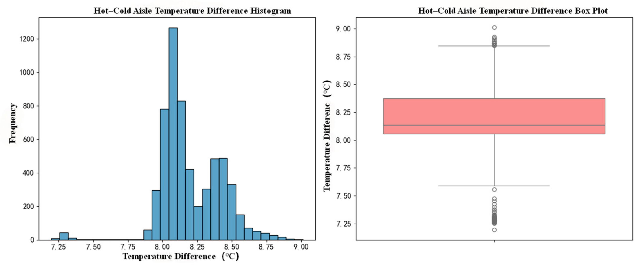
The overall hot–cold-aisle separation level is characterized by the hot–cold-aisle temperature difference. Statistical results show that the average temperature difference between hot and cold aisles is mainly concentrated within 8.0–8.5 °C, as shown in Figure 5. This indicates that the enclosed cold-aisle room can maintain relatively stable hot–cold separation during most operating periods and that the overall thermal environment remains controllable. However, stable overall hot–cold separation does not mean that all local cold aisles are in the same thermal state. Differences in temperature fluctuation among cold aisles should therefore be further analyzed.

3.2.2. Temperature Fluctuation Characteristics of Different Cold Aisles

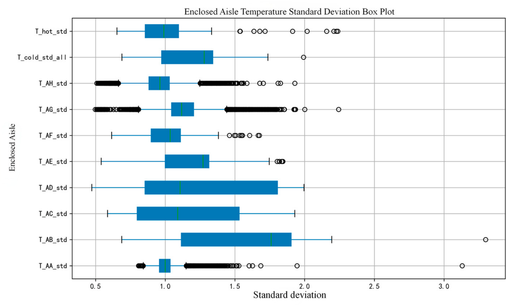
The stability of temperatures in different cold aisles was further compared, and obvious differences in thermal environment among aisles were observed. As shown in Figure 6, the AA and AH aisles show weaker temperature fluctuations and relatively stable operating states. The AB aisle has the highest mean standard deviation, a large interquartile range, and many high-value outliers, indicating more pronounced local temperature fluctuations and abnormal characteristics. The AD aisle also shows relatively weak stability. These results indicate that, even when the overall hot–cold separation level is relatively stable, local cold aisles may still be affected by differences in airflow distribution, IT-load distribution, and air-conditioning response, resulting in pronounced local temperature fluctuations.
Considering temperature-fluctuation level, local abnormal characteristics, and engineering relevance, this study selects the maximum temperature of cold-aisle AB as the subsequent prediction target. This variable can reflect local hotspot risk in the cold aisle and has direct engineering significance for precision air-conditioning regulation and thermal-safety control in data centers.

3.3. Predictor Analysis and Sample Construction

After determining the maximum temperature of cold-aisle AB as the prediction target, the main variables affecting target-temperature variation and their temporal action ranges need to be clarified. Considering the clear dynamic lag characteristics of temperature variation in enclosed cold-aisle rooms, this study analyzes variables from three perspectives: active air-conditioning control variables, heat-source-side disturbance variables, and cold-aisle state variables. Supervised-learning samples are then constructed based on the analysis results.

3.3.1. Lag Response Analysis of Cold-Aisle Temperature

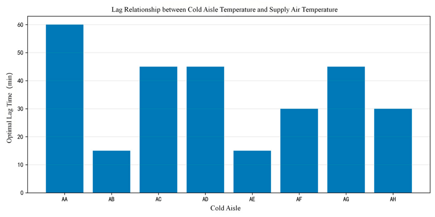
In data-center thermal management, the supply air temperature is a primary active control variable, whereas the maximum cold-aisle temperature serves as a key thermal-environment constraint. The two variables do not vary synchronously but exhibit a certain time lag due to the combined effects of equipment heat dissipation, airflow transport, and structural thermal inertia. To identify the short-term thermal response timescale of the enclosed cold-aisle data-center room under stable operating conditions, continuous operating data with complete monitoring records from 1 June 2025 were selected, and lag-correlation analysis was conducted between the supply air temperature and hotspot temperature for eight cold aisles, as shown in Figure 7. This analysis was primarily used to identify the dominant time range of the cold-aisle temperature response and to provide a reference for determining the historical input window in the subsequent prediction model.
In the analysis, the maximum value among temperature monitoring points in each cold aisle was used as the hotspot temperature characteristic of that aisle. The lagged Pearson correlation coefficient was used to quantify the coupling strength between supply air temperature and target temperature, and the optimal lag step was searched over the range of 0–180 min. As shown in Figure 7, the optimal lag times differ substantially among cold aisles. The AA aisle has the slowest response, at 60 min; the AB and AE aisles have the fastest response, at 15 min; the AC, AD, and AG aisles have a lag of 45 min; and the AF and AH aisles have a lag of 30 min.
As shown by the peak correlation coefficients in Table 1, notable differences exist among the cold aisles in both response speed and coupling strength to supply air disturbances. Longer lag times are generally associated with lower correlation coefficients, indicating that supply air paths, local airflow organization, and thermal inertia may influence the response process. For cold-aisle AB, the optimal lag time is 15 min, with a peak correlation coefficient of 0.66, indicating a relatively rapid response to supply air variations. Considering that lag characteristics may vary with IT load and air-conditioning operating conditions, this analysis is used only to identify the dominant timescale of the thermal response, rather than treating the optimal lag obtained from a single day as a fixed model parameter. Overall, the dominant lag times of the cold aisles are concentrated within 15–60 min. Therefore, a 120 min historical window is adopted in the subsequent modeling to cover the main response range and its persistent effects.

3.3.2. Influencing-Factor Screening

The preceding analysis indicates that cold-aisle temperature exhibits a time lag on the order of minutes in response to supply air regulation, with differences in response time among individual cold aisles. On this basis, to further identify the main factors influencing the maximum temperature in cold-aisle AB, the correlations between the historical states of the candidate variables and the target temperature are analyzed. This study first selects candidate variables from the previous one to three time steps for correlation analysis to identify the dominant factors. On this basis, subsequent sample construction is further extended to the most recent eight historical time steps to cover a more complete thermal-response process.
According to the room heat-transfer process, variables affecting the target temperature mainly include heat-source-side variables, control-side variables, and cold-aisle state variables. The heat-source-side variable is IT load; the control-side variables include supply air temperature, return air temperature, air velocity ratio, and the number of operating air-conditioning units; and the cold-aisle state variables include the maximum cold-aisle temperature and the standard deviation of cold-aisle temperature. Pearson correlation coefficients were used to analyze the linear relationships between the candidate variables and the maximum temperature of cold-aisle AB. The results are shown in Table 2.
The results show that the correlations between the ITload at the previous 1–3 time steps and the target temperature range from 0.89 to 0.90, indicating a strong statistical association. The lagged values of the target temperature itself all exhibit correlation coefficients of 0.96, reflecting pronounced temporal persistence. The standard deviation of the cold-aisle temperature is also highly correlated with the target temperature, suggesting a strong relationship between the local temperature distribution and variations in the maximum temperature. The number of operating air-conditioning units shows a strong negative correlation with the target temperature, reflecting the coupled effects of temperature conditions, load level, and air-conditioning regulation. The fan-speed ratio and supply air temperature exhibit certain linear correlations with the target temperature, whereas the Pearson correlation coefficient of the return air temperature is relatively low, indicating a weaker linear statistical association.
Considering the Pearson correlation results, heat-transfer mechanisms within the data-center room, the information characteristics of the variables, and their online availability, ITload, TAB_max, TAB_std, N, V, and Tsupply are ultimately selected as the model input variables. In this process, Pearson correlation analysis is mainly used to characterize the linear relationships between the candidate variables and the target temperature, while the model further learns more complex coupling relationships among the input variables through nonlinear feature extraction. The subsequent sample construction is extended to the most recent eight historical time steps to cover a more complete short-term thermal response process.

3.3.3. Input Window and Sample Reconstruction

The thermal environment of an enclosed cold-aisle data-center room exhibits clear temporal continuity, and the operating state at a single time step cannot fully characterize the influence of preceding thermal conditions on subsequent temperature variations. The preceding analysis shows that the dominant response lags of different cold aisles to supply air disturbances are mainly concentrated within 15–60 min, while heat accumulation and airflow redistribution may cause the temperature effects to persist for a longer period. Therefore, the historical observation range is appropriately extended beyond the dominant lag interval to retain more complete information on short-term thermal evolution.
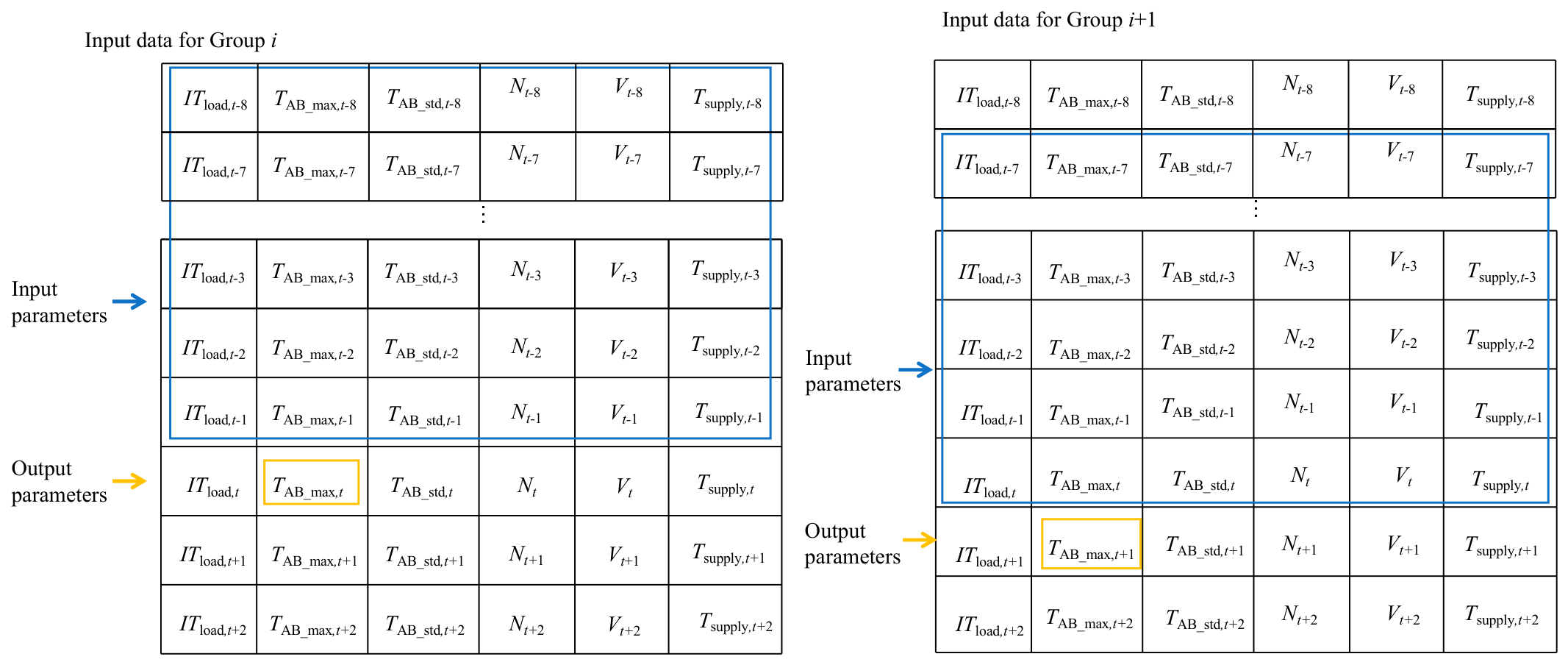
In this study, supervised-learning samples are constructed using a sliding time window, as shown in Figure 8. For the target time step (t), ITload, TAB_max, TAB_std, N, V, and Tsupply from the eight historical time steps, t − 8 to t – 1, are used as model inputs to predict the maximum temperature in cold-aisle AB at time, t, as shown in Figure 8. With a sampling interval of 15 min, each input window covers 120 min of historical operating information, resulting in an input matrix of 8 × 6. Accordingly, the prediction task established in this study uses the operating conditions over the preceding 120 min to predict the maximum temperature in cold-aisle AB 15 min ahead.
To ensure independence among the training, validation, and test sets, the eight-step historical windows were constructed separately within each data subset, without generating input-output sequences across dataset boundaries. After windowing, the training, validation, and test sets contained 4108, 580, and 1168 supervised-learning samples, respectively. The training set was used for model parameter learning, the validation set for hyperparameter tuning and early-stopping decisions, and the test set solely for the final evaluation of prediction performance.

3.4. Prediction Model Development

3.4.1. Problem Formulation

The prediction of the maximum temperature in cold-aisle AB is formulated as a one-step-ahead time-series prediction problem. For the target time step, t, the input feature vector at a historical time step, t − i, is expressed as follows:
x t - i = [ I T load , t i , T AB _ max , t i , T AB _ s t d , t i , N t i , V t i , T supply , t i ]
where ITload is the IT load, TAB_max is the maximum temperature of cold-aisle AB, TAB_std is the standard deviation of cold-aisle temperature, N is the number of operating precision air-conditioning units, V is the air velocity ratio, and Tsupply is the supply air temperature. Based on the preceding lag-correlation analysis and historical window setting, the model uses data from eight consecutive sampling time steps preceding the target time as input. Therefore, the t-th sample can be expressed as follows:
X t = x t 8 , x t 7 , , x t 1 8 × 6 , y t = T AB _ max ( t )
where X t is the temporal input matrix of the t-th sample, and y t is the prediction target at time t.
The model task can be expressed as learning the mapping relationship:
y t = f ( X t )
where f(·) denotes the constructed prediction model.

3.4.2. Model Architecture

This study develops a TSception–Transformer–TCN model for predicting the maximum cold-aisle temperature. The model takes six operating variables from eight consecutive sampling time steps preceding the target time as input, resulting in an input tensor of 8 × 6. The prediction target is TAB_max at the next sampling time step.
The input sequence is first processed by three parallel multi-scale depthwise separable convolution branches with temporal kernel sizes of 3, 5, and 7, respectively. Each branch contains 64 output channels and uses same padding and the ReLU activation function. The outputs of the three branches are concatenated along the feature dimension to obtain multi-scale temporal features with a dimension of 8 × 192. These features are then fed into the Transformer encoder module, where an eight-head self-attention mechanism, residual connections, and layer normalization are employed to enable cross-temporal information interaction within the historical window. After Transformer encoding, both the temporal and feature dimensions remain unchanged.
The Transformer output is subsequently fed into the downstream temporal convolution module. This module consists of two one-dimensional convolutional layers, each with a kernel size of 3 and 128 output channels, together with residual connections for feature propagation. After the first temporal convolutional layer, max pooling is applied to reduce the temporal dimension. The second convolutional layer further extracts local dynamic features, after which global average pooling is used to obtain a fixed-length feature vector. Finally, the vector is passed through a fully connected layer to output the predicted value of TAB_max.

3.4.3. Model Training and Evaluation Metrics

The proposed model is trained using the Adam optimizer with an initial learning rate of 0.001. Mean squared error (MSE) is used as the loss function, with a batch size of 32 and a maximum of 50 training epochs. During training, the validation loss is used as the criterion for model selection. Early stopping is applied when the validation loss does not improve for 10 consecutive epochs, and the model parameters corresponding to the lowest validation loss are restored.
BP (Back-Propagation) neural network, LSTM neural network, and XGBoost are selected as baseline models, representing a conventional feedforward neural network, a recurrent time-series model, and an ensemble tree-based learning method, respectively. All models use the same dataset partitioning, input variables, historical window, and prediction target. Specifically, six operating variables from the eight sampling time steps preceding the target time are used to predict the maximum temperature in cold-aisle AB at the next sampling time step. The LSTM and the proposed model take an 8 × 6 temporal matrix as input, whereas BP and XGBoost flatten the same historical window into a 48-dimensional feature vector to ensure consistency in the input information across different models. Model training is performed using the training set, while the main hyperparameters are determined based on validation-set performance. The test set is not involved in model selection or parameter tuning and is used exclusively for the final evaluation of prediction performance. The main parameter settings of each model are presented in Table 3.
For the ablation study, reduced-architecture models, including Transformer, TCN, Transformer–TCN, and TSception–TCN, are further constructed. Pairwise comparisons between corresponding model configurations are conducted to evaluate the incremental contributions of the TSception-based multi-scale feature extraction, Transformer-based cross-temporal information interaction, and TCN-based temporal feature integration modules to prediction performance. To reduce the variability in results caused by random initialization and the training process, each model is independently trained and evaluated using five different random seeds to assess both prediction performance and stability.
To evaluate the 15 min one-step-ahead prediction performance of each model for the maximum temperature in cold-aisle AB, four metrics are adopted: mean absolute error (MAE), root mean square error (RMSE), normalized root mean square error (NRMSE), and mean absolute percentage error (MAPE). MAE and RMSE are used to quantify absolute prediction errors, whereas MAPE characterizes the relative prediction error. NRMSE normalizes RMSE by the range of the actual temperature values, thereby reducing the influence of units and data scales on the evaluation results and improving comparability across different prediction targets and datasets.
MAE = 1 n i = 1 n | y i y ^ i |
RMSE = 1 n i = 1 n ( y i y ^ i ) 2
NRMSE = RMSE y max y min × 100 %
MAPE = 1 n i = 1 n y i y ^ i y i × 100 %
where y i is the measured temperature of the i-th data sample; y ^ i is the predicted temperature of the i-th data sample; n is the total number of samples in the dataset; and ymax and ymin denote the maximum and minimum actual temperatures in the evaluation dataset, respectively. MAE and RMSE are expressed in °C, NRMSE is dimensionless, and MAPE is expressed as a percentage. For all the above metrics, lower values indicate higher prediction accuracy.

4. Results and Discussion

4.1. Comparison of Prediction Performance Among Baseline Models

To compare the performance of different models in the cold-aisle temperature-prediction task, Persistence, BP, LSTM, and XGBoost were introduced as baseline models and compared with the proposed TSception–Transformer–TCN model. The Persistence model directly uses the most recent measured maximum temperature of cold-aisle AB before the prediction time as the predicted value for the next 15 min time step, i.e., T ^ A B _ max , t + 1 = T A B _ max , t , and is used to evaluate the performance improvement of the proposed model over the short-term persistence of temperature. All models used the same test period and prediction target, and the trainable models were independently evaluated using five different random seeds. The results are presented in Table 4.
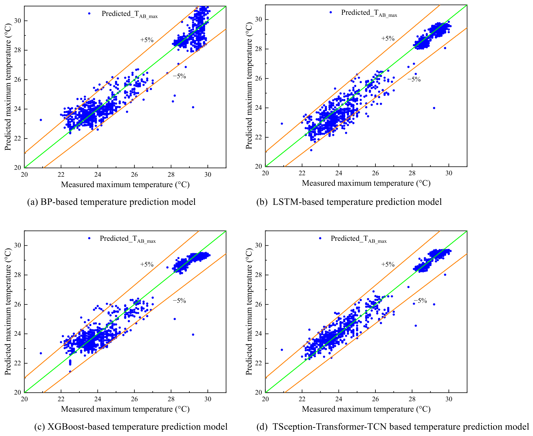
The results show that the Persistence model achieved an MAE of 0.539 °C and an RMSE of 0.781 °C, outperforming the BP model. This indicates that the maximum cold-aisle temperature exhibits strong short-term continuity and that using the most recent temperature measurement alone can already provide a certain level of prediction accuracy. The proposed model achieves the lowest MAE, RMSE, NRMSE, and MAPE values among the compared models. Compared with BP and LSTM, XGBoost demonstrates better prediction performance, indicating that ensemble-learning methods can effectively characterize the nonlinear relationships between operating parameters and cold-aisle temperature. On this basis, the TSception–Transformer–TCN model further reduces the prediction errors, suggesting that multi-scale temporal feature extraction and dependency modeling of historical operating states contribute to improved short-term temperature-prediction accuracy.
To further compare the agreement between the predicted and actual temperatures obtained by different models, Figure 9 presents scatter plots of the predicted values against the actual values for each model. The diagonal line represents the ideal condition in which the predicted values exactly match the actual values. A higher concentration of data points around this line indicates a smaller prediction deviation. It can be observed that all models are able to capture the overall variation in the maximum temperature of cold-aisle AB, although clear differences exist in the dispersion of the data points. The predictions of the BP model are relatively scattered, with some samples deviating considerably from the ideal prediction line. The scatter points of LSTM and XGBoost show a higher degree of concentration, whereas the predictions of the proposed model are generally more closely distributed around the ideal prediction line, consistent with the error-evaluation results presented in Table 4.

4.2. Ablation Study and Structural Contribution Analysis

To analyze the effects of individual functional modules on prediction performance, reduced-architecture models, including Transformer, TCN, TSception–TCN, and Transformer–TCN, are constructed and evaluated through multiple independent experiments under the same dataset partitioning and training conditions. The ablation study results are presented in Table 5. The standalone Transformer and TCN models exhibit comparable prediction performance, with MAE values of 0.528 ± 0.005 °C and 0.519 ± 0.004 °C, and RMSE values of 0.714 ± 0.006 °C and 0.716 ± 0.004 °C, respectively. Compared with the subsequent hybrid models, both standalone architectures show higher prediction errors, indicating that a single temporal modeling mechanism has limited capability to characterize the dynamic features of cold-aisle temperature.
After introducing TSception into the TCN architecture, the MAE of TSception–TCN decreases from 0.519 °C to 0.482 °C, while the RMSE decreases from 0.716 °C to 0.675 °C, indicating that multi-scale convolution facilitates the extraction of temperature variation features over different historical time ranges. The MAE and RMSE of Transformer–TCN further decrease to 0.468 °C and 0.663 °C, respectively, suggesting that the self-attention mechanism and downstream temporal feature integration provide complementary benefits for this prediction task.
The complete TSception–Transformer–TCN model achieves the lowest prediction errors, with MAE, RMSE, NRMSE, and MAPE values of 0.285 ± 0.003 °C, 0.438 ± 0.004 °C, 4.76 ± 0.05%, and 1.13 ± 0.02%, respectively. Compared with the best-performing reduced model, Transformer–TCN, the MAE, RMSE, NRMSE, and MAPE are reduced by approximately 39.1%, 33.9%, 34.0%, and 39.6%, respectively. Overall, the results of the reduced models indicate that multi-scale feature extraction, historical-state-dependency modeling, and downstream temporal feature integration all contribute positively to prediction performance, and their combination enables a more comprehensive representation of temperature dynamics.
The ablation results further reveal the contributions of the individual modules to prediction performance. The Transformer model is capable of capturing dependencies among different time steps within the historical window, but is less responsive to rapid local fluctuations and peak temperature variations. In contrast, the TCN model is more sensitive to local variations at adjacent time steps, but remains limited in representing cross-temporal dependencies. Therefore, when Transformer or TCN is used alone, it is difficult to fully characterize the rapid disturbances, regulation delays, and slowly varying thermal inertia that coexist in enclosed cold-aisle temperature sequences.
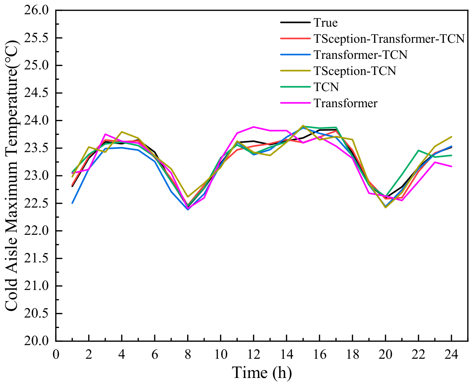
To intuitively illustrate the model’s ability to track continuous temperature variations, a continuous 24 h period containing temperature increases, decreases, and local fluctuations was selected from the test set for illustrative presentation, as shown in Figure 10. The predicted curve generally follows the overall trend of the actual temperature. Good agreement is maintained during relatively stable periods, while the model also tracks the actual temperature changes well during local warming and fluctuation periods. Together with the ablation results, these findings indicate that the complete model not only reduces the overall prediction error but also maintains good temperature-tracking performance during local dynamic variations.

4.3. Prediction Performance Analysis Across Different Cold Aisles

To evaluate the performance of the proposed model for cold-aisle temperature prediction at different spatial locations, seven additional cold aisles, namely AA, AC, AD, AE, AF, AG, and AH, are selected for supplementary testing. For each cold aisle, its maximum temperature is taken as the prediction target, while the corresponding maximum temperature and temperature standard deviation are used as the historical-state features. The remaining input variables include IT load, number of operating precision air-conditioning units, fan-speed ratio, and average supply air temperature. The same eight-step historical window and 15 min one-step-ahead prediction setting used for cold-aisle AB are adopted for all cold aisles.
To ensure consistent experimental conditions across different cold aisles, the data for each aisle are chronologically divided into training, validation, and test sets at proportions of 70%, 10%, and 20%, respectively, without random shuffling. Min–Max normalization is applied to the input variables, with the normalization parameters determined solely from the corresponding training set of each cold aisle. The model architecture and main training parameters remain unchanged, and the model is trained and tested independently for each cold aisle. The prediction results are presented in Table 6.
The results show that prediction errors vary to some extent among different cold aisles. The MAE ranges from 0.129 to 0.227 °C, the RMSE from 0.165 to 0.345 °C, the NRMSE from 2.75% to 6.82%, and the MAPE from 0.51% to 0.98%, indicating that relatively low prediction errors are achieved for all cold aisles under the same model architecture and training settings. Among them, cold-aisle AC achieves the lowest MAE and MAPE, at 0.129 °C and 0.51%, respectively, whereas cold-aisle AF, AG, and AH exhibit relatively higher prediction errors. Combined with the preceding thermal-environment analysis, the differences in prediction performance among the cold aisles may be related to variations in temperature-fluctuation intensity and local airflow organization. Overall, all cold aisles maintain relatively low prediction errors, indicating that, within the same data-center room and under the same experimental settings, the proposed model is applicable to short-term prediction of the maximum cold-aisle temperature in different cold aisles.

4.4. Discussion

This study is based on actual operating data collected from a large-scale data center located in a hot-summer and warm-winter region. The experimental results demonstrate that the proposed model can effectively predict the maximum temperature in enclosed cold aisles. Because the dataset mainly covers relatively high-temperature operating conditions during summer, the temperature-response patterns learned by the model are closely related to the load characteristics, air-conditioning operating strategies, and airflow organization of the investigated data-center room. Therefore, the current results primarily reflect the prediction performance of the model under the specific conditions considered in this study, and its generalization capability under different climatic conditions, operating loads, and data-center configurations remains to be further validated. Meanwhile, the lag analysis conducted on a typical operating day shows that the dominant thermal response times are concentrated within 15–60 min, providing a basis for determining the historical input window. Nevertheless, the specific response time may vary under different operating conditions.
The maximum cold-aisle temperature directly reflects local high-temperature conditions and is strongly associated with hotspot risk, making it a suitable prediction target for thermal-safety-oriented short-term forecasting. However, a single maximum-temperature indicator cannot fully characterize the overall thermal environment of a cold aisle, and its prediction cannot replace a comprehensive evaluation involving average temperature, temperature uniformity, and spatial temperature distribution. The independent modeling results for different cold aisles further indicate that the proposed architecture can be applied to the prediction of multiple temperature time series within the same data-center room. However, because the model is retrained separately using the data from each cold aisle, the current results do not yet demonstrate its spatial transferability to previously unseen cold aisles.
From an engineering application perspective, this study achieves 15 min one-step-ahead prediction of the maximum cold-aisle temperature, providing predictive information for short-term perception of the thermal environment in the data-center room. The model consists of multi-scale convolution, self-attention, and temporal convolution modules, and its practical deployment requires comprehensive consideration of model size, computational cost, inference latency, and hardware resource requirements. Future work will expand data coverage across different seasons, data centers, and operating conditions; further evaluate cross-aisle generalization and computational performance; and incorporate multiple indicators, including the average cold-aisle temperature, temperature dispersion, and spatial temperature distribution, to explore the application of the prediction results to hotspot-risk identification and coordinated control of precision air-conditioning systems.

5. Conclusions and Future Work

This study addresses short-term prediction of the maximum cold-aisle temperature in an enclosed cold-aisle data-center room. Using actual operational monitoring data from a large data center located in a hot-summer and warm-winter region, thermal-environment characterization, influencing-factor screening, sample construction, and model prediction are conducted. A hybrid prediction model integrating TSception, Transformer, and TCN is developed. The main conclusions are as follows:
(1)
Temperature variation in enclosed cold-aisle data-center rooms shows clear spatial heterogeneity and temporal lag. Thermal-environment analysis indicates that the average temperature difference between hot and cold aisles is mainly concentrated within 8.0–8.5 °C, suggesting that the overall hot–cold separation is relatively stable. However, temperature fluctuations differ markedly among cold aisles. Cold-aisle AB exhibits relatively high temperature dispersion, with more pronounced local temperature fluctuations. The lag-correlation analysis shows that the dominant response times of the cold aisles to changes in supply air temperature are concentrated within 15–60 min, indicating that historical operating states play an important role in short-term prediction of the maximum cold-aisle temperature.
(2)
For the 15 min one-step-ahead prediction of the maximum temperature in cold-aisle AB, the proposed model achieves an MAE of 0.285 °C, an RMSE of 0.438 °C, an NRMSE of 4.76%, and a MAPE of 1.13%, outperforming the baseline models, including Persistence, BP, LSTM, and XGBoost. The prediction results indicate that the proposed model can effectively characterize the short-term dynamic variations in the maximum cold-aisle temperature and improve prediction accuracy during periods of local temperature fluctuations.
(3)
Considering the coexistence of variations across multiple timescales and historical-state dependencies in cold-aisle temperature sequences, the proposed model jointly characterizes temperature dynamics through multi-scale local feature extraction, historical-state-dependency modeling, and temporal feature integration. The ablation results show that introducing the individual functional modules improves prediction performance over the corresponding reduced architectures, while the complete model achieves the lowest prediction error. This demonstrates the complementary effects of multi-scale feature extraction, the self-attention mechanism, and temporal feature integration in the present prediction task.
(4)
With the model architecture, input variable types, and training procedure kept consistent, independent modeling is further conducted for cold-aisle AA, AC, AD, AE, AF, AG, and AH, with MAPE values below 1% for all aisles. The results indicate that the proposed model architecture maintains low prediction errors in independent temperature-prediction tasks for different cold aisles within the same data-center room, demonstrating good applicability to multi-aisle modeling.
Future research will focus on three aspects: data coverage, spatial generalization, and engineering applications. The current study is primarily based on data collected from a single data center, with samples mainly covering relatively high-temperature operating conditions. Therefore, the data coverage remains limited in terms of seasonal variations, climatic regions, load levels, and data-center configurations. Meanwhile, the lag-correlation analysis conducted in this study is based on operating data from a limited period, and the identified response characteristics may be affected by specific load levels and operating conditions. Thus, the representativeness and robustness of the lag characteristics require further validation. Future studies will expand the dataset to include different seasons, climatic regions, load levels, and data-center configurations, and conduct lag-correlation analysis over longer periods and under diverse operating conditions to further evaluate the stability of historical-window selection and the generalization capability of the proposed method in complex operating scenarios. In addition, leave-one-cold-aisle-out validation and cross-cold-aisle transfer testing will be performed to investigate the spatial generalization capability of the model for cold aisles not involved in training. Multi-indicator prediction incorporating average temperature, temperature dispersion, and spatial temperature distribution information will also be explored to achieve a more comprehensive characterization of the thermal environment. Finally, the model size, computational cost, inference latency, and hardware resource requirements will be further evaluated. The integration of the proposed model with optimization and control strategies for precision air-conditioning systems will be investigated to support online thermal-environment prediction and operational regulation.

Author Contributions

Conceptualization, Z.Y. and X.Z.; methodology, Z.Y. and X.Z.; validation, M.W.; formal analysis, Z.Y. and M.W.; investigation, Z.Y.; resources, J.Y.; writing—original draft, Z.Y.; writing—review and editing, J.Y., X.Z. and M.W.; supervision, J.Y.; funding acquisition, J.Y. All authors have read and agreed to the published version of the manuscript.

Funding

This research received no external funding.

Data Availability Statement

The original contributions presented in this study are included in the article.

Conflicts of Interest

The authors declare no conflicts of interest.

References

  1. Chu, W.; Wang, C. A Review on Airflow Management in Data Centers. Appl. Energy 2019, 240, 84–119. [Google Scholar] [CrossRef] [Scilit]
  2. Jao, Y.; Zhang, Z.; Wang, C. Effect of Uneven Heat Load on the Airflow Uniformity and Thermal Performance in a Small-Scale Data Center. Appl. Therm. Eng. 2024, 242, 122525. [Google Scholar] [CrossRef] [Scilit]
  3. Meng, X.; Zhou, J.; Zhang, X.; Luo, Z.; Gong, H.; Gan, T. Optimization of the Thermal Environment of a Small-Scale Data Center in China. Energy 2020, 196, 117080. [Google Scholar] [CrossRef] [Scilit]
  4. Song, P.; Zhang, Z.; Zhu, Y. Numerical and Experimental Investigation of Thermal Performance in Data Center with Different Deflectors for Cold Aisle Containment. Build. Environ. 2021, 200, 107961. [Google Scholar] [CrossRef] [Scilit]
  5. Lee, Y.; Wen, C.; Shih, Y.; Li, Z.; Yang, A.-S. Numerical and Experimental Investigations on Thermal Management for Data Center with Cold Aisle Containment Configuration. Appl. Energy 2022, 307, 118213. [Google Scholar] [CrossRef] [Scilit]
  6. Athavale, J.; Yoda, M.; Joshi, Y. Comparison of Data Driven Modeling Approaches for Temperature Prediction in Data Centers. Int. J. Heat Mass Transf. 2019, 135, 1039–1052. [Google Scholar] [CrossRef] [Scilit]
  7. Guo, H.-B.; Chen, J.-Y.; Li, Z.-D.; Liu, X.-H.; Li, N.; Tao, W.-Q. FNM-Based Rack Model and CFD-FNM Coupling Framework for Data Center Rack-Level Simulation. Build. Environ. 2025, 272, 112675. [Google Scholar] [CrossRef] [Scilit]
  8. Singh, N.; Permana, I.; Agharid, A.P.; Wang, F.J. Innovative Retrofits for Enhanced Thermal Performance in Data Centers Using Independent Row-Based Cooling Systems. Therm. Sci. Eng. Prog. 2025, 57, 103101. [Google Scholar] [CrossRef] [Scilit]
  9. Szeliga, W.; Oleksiak, A.; Roszak, R.; Górzeński, R. CFD4DC: Automated CFD Framework for Heat Transfer Analysis of Data Centers. Appl. Therm. Eng. 2026, 283, 128982. [Google Scholar] [CrossRef] [Scilit]
  10. Wang, N.; Guo, Y.; Huang, C.; Tian, B.; Shao, S. Multi-Scale Collaborative Modeling and Deep Learning-Based Thermal Prediction for Air-Cooled Data Centers: An Innovative Insight for Thermal Management. Appl. Energy 2025, 377, 124568. [Google Scholar] [CrossRef] [Scilit]
  11. Xu, W.; Zhao, B.; Zeng, Y.; Wang, T. Intelligent Data Center Safety Status Prediction Based on Algorithm Ensemble. In Proceedings of the 2023 International Conference on Mobile Internet, Cloud Computing and Information Security (MICCIS), Nanjing, China, 7–9 April 2023; pp. 63–68. [Google Scholar]
  12. Patel, D.; Joshi, Y. Data Driven Modeling Advancements for Air Temperature Predictions in Data Centers. Numer. Heat Transf. Part B Fundam. 2025, 86, 244–261. [Google Scholar] [CrossRef] [Scilit]
  13. Deng, P.; Xu, Q.; Zhu, X.; Dong, W. CFD-Based Data Driven Machine Learning Temperature Prediction: Case Study on a 180-Rack Server Room within a Large-Scale Data Center. Int. J. Therm. Sci. 2026, 221, 110465. [Google Scholar] [CrossRef] [Scilit]
  14. Lin, J.; Lin, W.; Lin, W.; Wang, J.; Jiang, H. Thermal Prediction for Air-Cooled Data Center Using Data Driven-Based Model. Appl. Therm. Eng. 2022, 217, 119207. [Google Scholar] [CrossRef] [Scilit]
  15. Asgari, S.; Moazamigoodarzi, H.; Tsai, P.J.; Pal, S.; Zheng, R.; Badawy, G.; Puri, I.K. Hybrid Surrogate Model for Online Temperature and Pressure Predictions in Data Centers. Future Gener. Comput. Syst. 2021, 114, 531–547. [Google Scholar] [CrossRef] [Scilit]
  16. Asgari, S.; MirhoseiniNejad, S.; Moazamigoodarzi, H.; Gupta, R.; Zheng, R.; Puri, I.K. A Gray-Box Model for Real-Time Transient Temperature Predictions in Data Centers. Appl. Therm. Eng. 2021, 185, 116319. [Google Scholar] [CrossRef] [Scilit]
  17. Lloyd, R.; Rebow, M. Data Driven Prediction Model (DDPM) for Server Inlet Temperature Prediction in Raised-Floor Data Centers. In Proceedings of the 2018 17th IEEE Intersociety Conference on Thermal and Thermomechanical Phenomena in Electronic Systems (ITherm), San Diego, CA, USA, 29 May–1 June 2018; pp. 716–725. [Google Scholar]
  18. Wang, S.; Ma, C.; Xu, Y.; Wang, J.; Wu, W. A Hyperparameter Optimization Algorithm for the LSTM Temperature Prediction Model in Data Center. Sci. Program. 2022, 2022, 6519909. [Google Scholar] [CrossRef] [Scilit]
  19. Zhang, L.; Zhang, L.; Li, Y.; Yan, L.; Zhang, N.; Lin, X. Cooling Load Prediction for Data Center Based on Re-LSTM. In Proceedings of the 2023 IEEE 7th Conference on Energy Internet and Energy System Integration (EI2), Hangzhou, China, 15–18 December 2023; pp. 3415–3420. [Google Scholar]
  20. Sha, Q.; Yang, J.; Shao, R.; Wang, Y. Prediction of Air-Conditioning Outlet Temperature in Data Centers Based on Graph Neural Networks. Energies 2025, 18, 1803. [Google Scholar] [CrossRef] [Scilit]
  21. Vaswani, A.; Shazeer, N.; Parmar, N.; Uszkoreit, J.; Jones, L.; Gomez, A.N.; Kaiser, L.; Polosukhin, I. Attention is All You Need. In Advances in Neural Information Processing Systems; The MIT Press: Cambridge, MA, USA, 2017; Volume 30. [Google Scholar]
  22. Lin, Y.; Koprinska, I.; Rana, M. Temporal Convolutional Attention Neural Networks for Time Series Forecasting. In Proceedings of the 2021 International Joint Conference on Neural Networks (IJCNN), Shenzhen, China, 18–22 July 2021; pp. 1–8. [Google Scholar]
  23. Wan, J.; Xia, N.; Yin, Y.; Pan, X.; Hu, J.; Yi, J. TCDformer: A Transformer Framework for Non-Stationary Time Series Forecasting Based on Trend and Change-Point Detection. Neural Netw. 2024, 173, 106196. [Google Scholar] [CrossRef] [Scilit] [PubMed]
  24. Ismail Fawaz, H.; Lucas, B.; Forestier, G.; Pelletier, C.; Schmidt, D.F.; Weber, J.; Webb, G.I.; Idoumghar, L.; Muller, P.-A.; Petitjean, F. InceptionTime: Finding AlexNet for Time Series Classification. Data Min. Knowl. Discov. 2020, 34, 1936–1962. [Google Scholar] [CrossRef] [Scilit]
  25. Liu, S.; Yu, H.; Liao, C.; Li, J.; Lin, W.; Liu, A.X.; Dustdar, S. Pyraformer: Low-Complexity Pyramidal Attention for Long-Range Time Series Modeling and Forecasting. In Proceedings of the International Conference on Learning Representations (ICLR), Virtual, 3–7 May 2021. [Google Scholar]
  26. Lea, C.; Flynn, M.D.; Vidal, R.; Reiter, A.; Hager, G.D. Temporal Convolutional Networks for Action Segmentation and Detection. In Proceedings of the 2017 IEEE Conference on Computer Vision and Pattern Recognition (CVPR); IEEE: New York City, NY, USA, 2017; pp. 156–165. [Google Scholar]
  27. Ding, Y.; Robinson, N.; Zhang, S.; Zeng, Q.; Guan, C. TSception: Capturing Temporal Dynamics and Spatial Asymmetry From EEG for Emotion Recognition. IEEE Trans. Affect. Comput. 2023, 14, 2238–2250. [Google Scholar] [CrossRef] [Scilit]
  28. Bai, S.; Kolter, J.Z.; Koltun, V. An Empirical Evaluation of Generic Convolutional and Recurrent Networks for Sequence Modeling. arXiv 2018, arXiv:1803.01271. [Google Scholar]
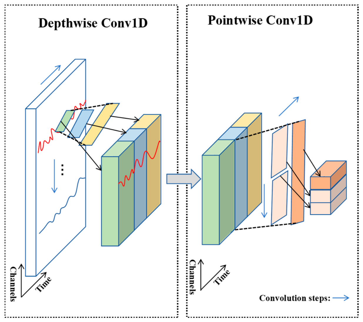
Figure 1. TSception-based multi-scale temporal feature-extraction architecture.
Buildings 16 03580 g001
Figure 2. Transformer encoder module architecture.
Buildings 16 03580 g002
Figure 3. Architecture of the TCN-based temporal feature integration module.
Buildings 16 03580 g003
Figure 4. Layout of the data-center room.
Buildings 16 03580 g004
Figure 5. Distribution of the overall hot–cold-aisle temperature difference.
Buildings 16 03580 g005
Figure 6. Box plot of standard deviation in enclosed cold aisles.
Buildings 16 03580 g006
Figure 7. Lag-correlation analysis between supply air temperature and T_max in each cold aisle.
Buildings 16 03580 g007
Figure 8. Sliding-window selection of input and output parameters.
Buildings 16 03580 g008
Figure 9. Predicted versus actual maximum cold-aisle temperatures for different models.
Buildings 16 03580 g009
Figure 10. Comparison of partial actual and predicted maximum temperatures in cold-aisle AB.
Buildings 16 03580 g010
Table 1. Lag-correlation analysis results for each cold aisle.
Maximum Cold-Aisle TemperaturePeak Correlation CoefficientLag Time (min)
TAE_max0.7215
TAH_max0.6730
TAB_max0.6615
TAD_max0.645
TAG_max0.5645
TAC_max0.5145
TAF_max0.4430
TAA_max0.3460
Table 2. Influence of different factors on the maximum temperature of cold-aisle AB.
Influencing FactorSymbolPearson Correlation Coefficient
IT load at the previous one, two, and three time stepsITload(t−1, t−2, t−3)0.89, 0.9, 0.9
Maximum cold-aisle AB temperature at the previous one, two, and three time stepsTAB_max(t−1, t−2, t−3)0.96, 0.96, 0.96
Cold-aisle AB temperature standard deviation at the previous one, two, and three time stepsTAB_std(t−1, t−2, t−3)0.84, 0.86, 0.86
Number of operating air-conditioning units at the previous one, two, and three time stepsN(t−1, t−2, t−3)−0.95, −0.94, −0.94
Air velocity ratio at the previous one, two, and three time stepsV(t−1, t−2, t−3)0.67, 0.67, 0.67
Supply air temperature at the previous one, two, and three time stepsTsupply(t−1, t−2, t−3)0.66, 0.62, 0.62
Return air temperature at the previous one, two, and three time stepsTreturn(t−1, t−2, t−3)0.03, 0.03, 0.03
Table 3. Main parameter settings of different models.
ModelMain Parameter Settings
BPHidden layers: 64–32; Activation: ReLU; Optimizer: Adam; Learning rate: 0.001
LSTM1 LSTM layer, 64 units; Dropout: 0.2; Optimizer: Adam; Learning rate: 0.001
XGBoostn_estimators: 300; max_depth: 4; learning_rate: 0.05; subsample: 0.8
TSception–Transformer–TCNKernel sizes: 3/5/7; Filters: 64; Attention heads: 8; key_dim: 64; TCN filters: 128; Optimizer: Adam; Learning rate: 0.001
Note: The batch size of BP, LSTM, and the proposed model was set to 32, with a maximum of 50 training epochs. Early stopping with a patience of 10 epochs was adopted for the neural-network-based models.
Table 4. Accuracy comparison of temperature-prediction models.
Prediction ModelMAE (°C)RMSE (°C)NRMSE (%)MAPE (%)
BP0.738 ± 0.0060.917 ± 0.0069.96 ± 0.072.85 ± 0.02
Persistence0.5390.7818.492.19
LSTM0.450 ± 0.0050.733 ± 0.0067.97 ± 0.061.79 ± 0.02
XGBoost0.356 ± 0.0040.519 ± 0.0045.64 ± 0.061.41 ± 0.02
TSception–Transformer–TCN0.285 ± 0.0030.438 ± 0.0044.76 ± 0.051.13 ± 0.02
Note: Persistence is a deterministic baseline and therefore is reported as a single value.
Table 5. Ablation study results of different model architectures.
Prediction ModelMAE (°C)RMSE (°C)NRMSE (%)MAPE (%)
Transformer0.528 ± 0.0050.714 ± 0.0067.77 ± 0.062.10 ± 0.02
TCN0.519 ± 0.0040.716 ± 0.0047.78 ± 0.052.07 ± 0.02
TSception–TCN0.482 ± 0.0040.675 ± 0.0057.35 ± 0.051.93 ± 0.02
Transformer–TCN0.468 ± 0.0040.663 ± 0.0057.21 ± 0.051.87 ± 0.02
TSception–Transformer–TCN0.285 ± 0.0030.438 ± 0.0044.76 ± 0.051.13 ± 0.02
Table 6. Comparison of temperature-prediction results for different cold aisles.
Cold AisleMAE (°C)RMSE (°C)NRMSE (%)MAPE (%)
AA0.1760.3454.600.72
AC0.1290.1652.750.51
AD0.1870.3176.470.74
AE0.1840.2604.730.72
AF0.2190.2884.720.85
AG0.2220.2906.400.87
AH0.2270.3076.820.98
Disclaimer/Publisher’s Note: The statements, opinions and data contained in all publications are solely those of the individual author(s) and contributor(s) and not of MDPI and/or the editor(s). MDPI and/or the editor(s) disclaim responsibility for any injury to people or property resulting from any ideas, methods, instructions or products referred to in the content.