Article

Intelligent Prediction of Subway Tunnel Settlement: A Novel Approach Using a Hybrid HO-GPR Model

College of Architecture Engineering, Xinjiang University, Urumqi 830049, China
*
Author to whom correspondence should be addressed.
Buildings 2026, 16(1), 192; https://doi.org/10.3390/buildings16010192 (registering DOI)
Submission received: 12 November 2025 / Revised: 20 December 2025 / Accepted: 23 December 2025 / Published: 1 January 2026
(This article belongs to the Section Construction Management, and Computers & Digitization)

Abstract

Precise prediction of structural settlement in subway tunnels is crucial for ensuring safety during both construction and operational phases; however, the non-linear characteristics of monitoring data pose a significant challenge to achieving this goal. To address this issue, this study proposes a hybrid predictive model, termed HO-GPR. This model integrates the Hippopotamus Optimization (HO) algorithm—a novel bio-inspired meta-heuristic—with Gaussian Process Regression (GPR), a non-parametric probabilistic machine learning method. Specifically, HO is utilized to globally optimize the hyperparameters of GPR to enhance its adaptability to complex deformation patterns. The model was validated using 52 months of field settlement monitoring data collected from the Urumqi Metro Line 1 tunnel. Through a series of comparative and generalization experiments, the accuracy and adaptability of the model were systematically evaluated. The results demonstrate that the HO-GPR model is superior to five benchmark models—namely Gated Recurrent Unit (GRU), Support Vector Regression (SVR), HO-optimized Back Propagation Neural Network (HO-BP), standard GPR, and ARIMA—in terms of accuracy and stability. It achieved a Coefficient of Determination (R2) of 0.979, while the Root Mean Square Error (RMSE), Mean Absolute Error (MAE), and Mean Absolute Percentage Error (MAPE) were as low as 0.318 mm, 0.240 mm, and 1.83%, respectively, proving its capability for effective prediction with non-linear data. The findings of this research can provide valuable technical support for the structural safety management of subway tunnels.

1. Introduction

With the growth of urban economies, industries, and populations, land resources in cities have become increasingly scarce. This has accelerated the construction of urban underground spaces, leading to a growing number of subway lines and drawing increasing attention to the safety of subway tunnels [1]. During the construction and operation of subway tunnels, the redistribution of surrounding rock stress and inevitable ground loss are the primary geotechnical mechanisms leading to structural settlement. Factors such as complex geological conditions, groundwater fluctuation, and train vibration loads further exacerbate the non-linear deformation of the tunnel structure. If this settlement is not accurately predicted and controlled, it can lead to segment cracking, leakage, or even catastrophic structural failure. Therefore, understanding these deformation mechanisms and establishing a precise prediction model is of significant engineering importance for safety management. Due to the uncertainty of these influencing factors and the complexity of the non-linear deformation, achieving accurate predictions of tunnel structural deformation is a significant challenge [2]. Therefore, developing high-precision prediction models capable of accurately capturing complex deformation patterns and identifying potential safety issues in advance is of great significance for disaster prevention and mitigation, risk prevention and control, and ensuring the operational safety of subways.
Various methods have been developed for settlement prediction, primarily categorized into numerical simulation [3], time series analysis [4], neural networks [5], and deep learning [6]. For instance, He et al. [7] established a time series model based on its fundamental principles, utilizing subway tunnel monitoring data to accurately forecast deformation trends. Wang et al. [8] introduced the Whale Optimization Algorithm (WOA) to optimize the parameters of a Back Propagation (BP) neural network, thereby constructing a WOA-BP model that enhanced the predictive capability for shield tunnel settlement. Similarly, Zhang et al. [9] employed an improved clustering method based on a Gaussian Mixture Model (GMM) to filter sensor data before using a Long Short-Term Memory (LSTM) network for settlement prediction. While these methods have demonstrated some efficacy, they each possess inherent limitations. The accuracy of numerical simulations, for instance, is often dependent on mesh quality and computational resources [10]. Time series models struggle to handle long-term dependencies in the data [11], while BP neural networks are often hindered by slow convergence speeds and a tendency to become trapped in local optima [12]. Furthermore, when processing raw settlement data, the capability of LSTM networks to mine underlying patterns and features is often constrained by the influence of various hidden factors within the data [13].
Advancing beyond these standalone models, the integration of Artificial Intelligence (AI) with Digital Twins (DT) has emerged as a transformative trend in the tunneling industry. For instance, Latif et al. [14] proposed a digital twin-driven framework to predict and monitor TBM performance through machine learning, while Sharafat et al. [15] utilized data-driven approaches for risk analysis in difficult ground conditions. However, despite these advancements, effective prediction typically requires large datasets, which are often unavailable in early construction stages. Furthermore, while Gaussian Process Regression (GPR) is theoretically suitable for small-sample predictions, its performance is heavily dependent on hyperparameter tuning. Traditional optimizers often struggle with the complex, non-convex loss functions of GPR, leading to premature convergence. This study addresses this specific gap. Unlike standard incremental improvements, the proposed model integrates the Hippopotamus Optimization (HO) algorithm not arbitrarily, but because its unique adaptive multi-strategy mechanism (including movement, evasion, and defense phases) effectively mitigates the local optima problem inherent in existing GPR models, thereby ensuring robust prediction under uncertainty.
With the maturation of data processing technologies, various machine learning methods have been applied to tunnel deformation monitoring [16]. Among these, Gaussian Process Regression (GPR), a non-parametric model based on Bayesian theory, has shown significant potential in the field of deformation prediction due to its distinct advantages in small-sample learning and handling non-linear problems [17]. For example, Liu et al. [18] developed a novel method that fuses a Grey Theory Model with GPR to predict ground surface deformation caused by subway construction. To improve model performance, Zheng et al. [19] introduced a differential evolution algorithm to optimize the key hyperparameters of GPR and incorporated the distance between the tunnel face and the monitoring section as a novel input feature. Xia et al. [20] proposed an improved GPR-based method for predicting the deformation of riverside foundation pits, providing a valuable reference for similar projects based on a case study of the Tianjin Metro Line 7. Addressing data quality, Zhang et al. [21] constructed a hybrid GF-GPR model by first employing a Gaussian Filter (GF) to denoise monitoring data before applying GPR for prediction, successfully demonstrating its application on a subway foundation pit at a station in Chengdu.
Despite the significant potential of GPR, its predictive accuracy and stability are highly dependent on the selection of its kernel function hyperparameters. Improper selection can degrade the model’s performance and lead to convergence at a local optimum [22]. To overcome this bottleneck, this study introduces the Hippopotamus Optimization (HO) algorithm to the GPR model. By leveraging the powerful global exploration and local exploitation capabilities of the HO algorithm to search for the optimal hyperparameters, a hybrid HO-GPR prediction model for subway tunnel deformation is constructed. The optimized GPR model is thus better equipped to capture the non-linear features of the data, enabling more precise predictions that closely approximate the true values. Based on measured settlement data from the section between Nanhu North Road Station and Wangjialiang Station of Urumqi Metro Line 1, this study compares the performance enhancement that different optimization algorithms offer to the GPR model. Subsequently, the effectiveness and applicability of the proposed model are validated through a comprehensive comparative analysis against other established models. The findings are intended to provide valuable technical support for deformation monitoring tasks in similar engineering projects.

2. An HO-GPR Model for Deformation Prediction

2.1. Hippopotamus Optimization Algorithm

The Hippopotamus Optimization (HO) algorithm is a novel bio-inspired meta-heuristic that mimics the behavioral patterns of hippopotamuses in their natural habitat [23]. The optimization process is mathematically modeled through three distinct phases: position update in the river, defense against predators, and evasion.

2.1.1. Movement Strategy

Hippopotamuses tend to aggregate in groups led by a dominant male. The position update is modeled based on the location of the dominant individual (the best solution found so far), formulated as:
x n e w ( t ) = x ( t ) + r 1 × ( x d o m ( t ) F × x ( t ) )
In the formula, x n e w ( t ) is the current position vector, x d o m ( t ) represents the position of the dominant hippopotamus, and F is a random integer (1 or 2) representing the aggregation factor. r 1 is a random vector with components uniformly distributed in [ 0 , 1 ] .

2.1.2. Defense Strategy

When threatened, hippopotamuses exhibit defensive behaviors within a limited range. This phase enhances the algorithm’s local exploitation capability:
x n e w ( t ) = x ( t ) + r 2 · ( x p r e ( t ) x ( t ) )
In the formula, x p r e is a randomly generated position within the search space representing the predator, and r 2 is a random vector in [ 0 , 1 ] .

2.1.3. Evasion Strategy

To avoid critical danger, the hippopotamus may flee to a random location. This mechanism is crucial for avoiding local optima:
x n e w ( t ) = l b + r 3 · ( u b l b )
In the formula, l b and u b denote the lower and upper bounds of the search space, respectively. r 3 is a random vector in [ 0 , 1 ] .
The training of a GPR model involves optimizing hyperparameters by maximizing the Log-Marginal Likelihood (LML). This optimization landscape is typically non-convex and multimodal, meaning standard gradient-based methods or simple meta-heuristics often get trapped in local optima. The HO algorithm is particularly suitable for this application because its adaptive multi-phase strategy balances global search and local refinement. The Evasion phase effectively prevents premature convergence, ensuring the algorithm can escape local optima in the GPR likelihood function, while the Defense phase ensures high-precision tuning of the hyperparameters.

2.2. Gaussian Process Regression

Gaussian Process Regression (GPR) is a non-parametric machine learning model rooted in Bayesian theory. It has gained widespread application due to its unique advantage of providing probabilistic predictions, particularly for problems involving small sample sizes and non-linear relationships. The core principle of GPR involves defining a prior distribution over the space of functions. This prior is then updated with observed data to yield a posterior distribution, which is subsequently used to make predictions for new, unseen data points.

2.2.1. Principle of GPR Prediction

The GPR model assumes that an observed value is the sum of the true function value and an independent noise term:
y = f ( x ) + ζ
In this study, the input vector x is constructed as [ y t 1 , y t 2 , Δ 2 y t 1 , t ] , where y t 1 and y t 2 represent the settlement values of the previous two periods; Δ 2 y t 1 is the second-order difference calculated as ( y t 1 y t 2 ) ( y t 2 y t 3 ) ; and t is the normalized time index. f ( x ) is the function value, y is the observed value, and ζ is the Gaussian white noise, ζ ~ N ( 0 , σ n 2 ) .
Since both f ( x ) and ζ follow a Gaussian distribution, it follows that the observed value y is also Gaussian distributed. For a set of training inputs X = { x i } i = 1 n the prior distribution over the corresponding observed values y is given by:
y ~ N 0 , K X , X + σ n 2 I n
In the formula, K X , X is the n × n kernel matrix computed by the kernel function, and I n is the identity matrix.
To define a prior over the function space for f ( x ) , a Gaussian Process (GP) is introduced. The function f ( x ) is a stochastic process where any finite collection of its variables follows a joint Gaussian distribution. A GP is completely determined by its mean function m ( x ) and kernel function k ( x , x ) . Therefore, the GP prior on the function f ( x ) can be expressed as:
f ( x ) ~ G P ( m ( x ) , k ( x , x ) )
In the formula, m ( x ) = E [ f ( x ) ] is the mean function, often assumed zero for simplicity. The kernel function, k ( x , x ) = E [ ( f ( x ) m ( x ) ) ( f ( x ) m ( x ) ) ] evaluates the correlation between the function values at any two points, x and x′.
With the prior established, the core of GPR prediction lies in determining the posterior predictive distribution. Given a training dataset D = { ( x i , y i ) } i = 1 n and new test inputs X , the goal is to compute the posterior probability distribution of the function values f ( X ) . This is achieved by establishing a joint prior distribution over the observed training outputs y and the predicted test outputs f ( X ) based on Bayesian principles. This joint distribution is also Gaussian and is expressed as follows:
y f ( X ) ~ N 0 , K ( X , X ) + s n 2 I n K ( X , X ) K ( X , X ) K ( X , X )
In the formula, K ( X , X ) is the n × n symmetric positive-definite covariance matrix computed from the training inputs, K ( X , X ) is the n × m covariance matrix between the training inputs X and the test inputs X , K ( X , X ) is the transpose of K ( X , X ) , and K ( X , X ) is the m × m covariance matrix of the test inputs.
By applying the rules of conditional probability to this joint Gaussian distribution, the posterior predictive distribution for the test outputs f ( X ) can be derived as follows:
f ( X ) | X , y , X ~ N ( m ( f ( X ) ) , c o v ( f ( X ) ) )
In the formula, where the predictive mean m ( f ( X ) ) provides the optimal estimate for the unknown output, and the predictive covariance, c o v f ( X ) quantifies the uncertainty of this prediction. The equations for calculating m f ( X ) and c o v f ( X ) are as follows:
m ( f ( X ) ) = K ( X , X ) [ K ( X , X ) + σ n 2 I n ] 1 y
c o v ( f ( X ) ) = K ( X , X ) K ( X , X ) [ K ( X , X ) + s n 2 I n ] 1 K ( X , X )

2.2.2. GPR Model Training

The training process of a GPR model is essentially the process of selecting a suitable kernel function and determining its optimal hyperparameters. The kernel function is crucial as it defines the covariance matrix, which ultimately determines both the model’s predictions and their associated variance. This variance serves as a measure of the confidence interval for the predictive results. In this study, a composite kernel function combining the Radial Basis Function (RBF) and the Periodic kernel is adopted. While the RBF kernel is effective at capturing the smooth, non-linear accumulation of plastic settlement (the primary structural trend), it may struggle to distinguish between random noise and regular environmental responses. However, monitoring data often exhibits periodic fluctuations superimposed on the cumulative settlement trend. To accurately capture these characteristics, a Periodic kernel is introduced alongside the RBF kernel. By constructing this composite kernel, the model can effectively decouple the irreversible structural trend from reversible environmental effects, thereby preventing the overfitting of seasonal variations as permanent deformation. The kernel function constructed in this paper is as follows:
k ( x i , x j ) = c · ( k RBF ( x i , x j ) + k Per ( x i , x j ) )
k Per x i , x j = σ 2 exp 2 sin 2 π d x i , x j P l p 2
k RBF x i , x j = σ 2 exp d ( x i , x j ) 2 2 l r 2
In the formula, c is the constant kernel, σ 2 is the signal variance, k x i , x j calculates the covariance between any two input points x i and x j , d represents the distance between them, l r , l p are the length-scale hyperparameters for the R B F (Radial Basis Function) and P e r (Periodic) kernels, respectively, and P is the period length. Additionally, σ n 2 represents the variance of the Gaussian noise. Together, these parameters constitute the hyperparameter set θ = c , l r , l p , P , σ n 2 to be optimized.
Traditional methods for solving for these hyperparameters, such as gradient-based conjugate gradient methods, typically rely on Maximum Likelihood Estimation (MLE). However, these methods are prone to converging at local optima. Therefore, this study adopts the HO algorithm to perform hyperparameter optimization. The HO algorithm searches for the optimal set of hyperparameters, θ, that maximizes the marginal log-likelihood function of the training data. This function is expressed as follows:
L ( θ ) = log ( p ( y | X , θ ) ) = 1 2 y T ( K + σ n 2 I n ) 1 y 1 2 log | K + σ n 2 I n | n 2 log 2 π
In the formula, y is the vector of observed values for the training set, X represents the corresponding training inputs, y T is the transpose of y, and K is the kernel matrix, determined by the set of hyperparameters θ = c , l r , l p , p , σ n 2 , where θ is the set of hyperparameters defined previously, I n is the n × n identity matrix, and n is the total number of training samples.

2.3. Construction of the HO-GPR Model

Introducing the Hippopotamus Optimization (HO) algorithm into the hyperparameter optimization process of the GPR model effectively addresses the issues of low prediction accuracy and poor stability [24], which often arise when traditional gradient-based methods become trapped in local optima. By leveraging its robust global search capabilities, the HO algorithm identifies the globally optimal combination of hyperparameters for the GPR kernel function. This process significantly enhances the predictive capability and reliability of the GPR model, leading to the establishment of a high-precision prediction model.
The specific optimization process involves several key steps. First, the operational parameters for the HO algorithm must be configured, including the population size, the maximum number of iterations, and the search boundaries for each GPR hyperparameter. Collectively, these parameters define the scale and scope of the optimization search. Next, an objective function is defined to effectively couple the HO algorithm with the GPR model. This function incorporates all necessary parameters for GPR training Crucially, to strictly preserve the temporal dependency and prevent data leakage, a Time Series Cross-Validation (TSCV) approach with an Expanding Window scheme is implemented within the objective function. Specifically, the data is divided into k = 3 chronological splits, where the model is trained on the first i segments and validated on the (i+1)-th segment, ensuring that the training set always precedes the validation set. Additionally, a temporal hold-out strategy is employed for final evaluation, isolating the last 16 data points solely for testing. The optimization goal being the minimization of the Mean Squared Error (MSE) [25]. The fitness function, defined by the MSE, is given by the following formula:
MSE = 1 n i = 1 n ( y i y ^ i ) 2
In the formula, y i and y ^ i are the true and predicted values for the i th sample, respectively.
Guided by this criterion, the HO algorithm explores the global search space. This process continues until the combination of hyperparameters that yields the lowest MSE value is identified; this combination is considered the global optimal solution. Finally, this optimal set of hyperparameters is applied to the GPR model to construct the performance-optimized HO-GPR prediction model. The application of the HO algorithm to the GPR model synergistically combines the global optimization capabilities of the former with the non-parametric modeling advantages of the latter, thereby enhancing the predictive performance and robustness of the GPR model. The specific construction steps of the proposed prediction model are illustrated in Figure 1.

2.4. Evaluation Metrics

To objectively and comprehensively evaluate the predictive performance of the HO-GPR model, four metrics were selected: the Coefficient of Determination (R2), Root Mean Square Error (RMSE), Mean Absolute Error (MAE), and Mean Absolute Percentage Error (MAPE) [26,27,28]. R2 reflects the goodness of fit of the model; a value closer to 1 indicates a stronger ability to fit the actual data and thus a better predictive performance. Conversely, for RMSE, MAE, and MAPE, lower values are better. Values closer to 0 signify a smaller error between the true and predicted values, indicating higher prediction accuracy. The formulas for these metrics are as follows:
R 2 = 1 i = 1 n ( y i y ^ i ) 2 i = 1 n ( y i y ¯ ) 2
RMSE = i = 1 n ( y ^ i y i ) 2 n
MAE = 1 n i = 1 n y i y ^ i
MAPE = 1 n i = 1 n y ^ i y i y i × 100 %
In the formula, y i is the true value of the i th sample, y ^ i is the predicted value for the i th sample, y ¯ is the mean of all true values, and n is the total number of samples.

3. Case Study and Validation

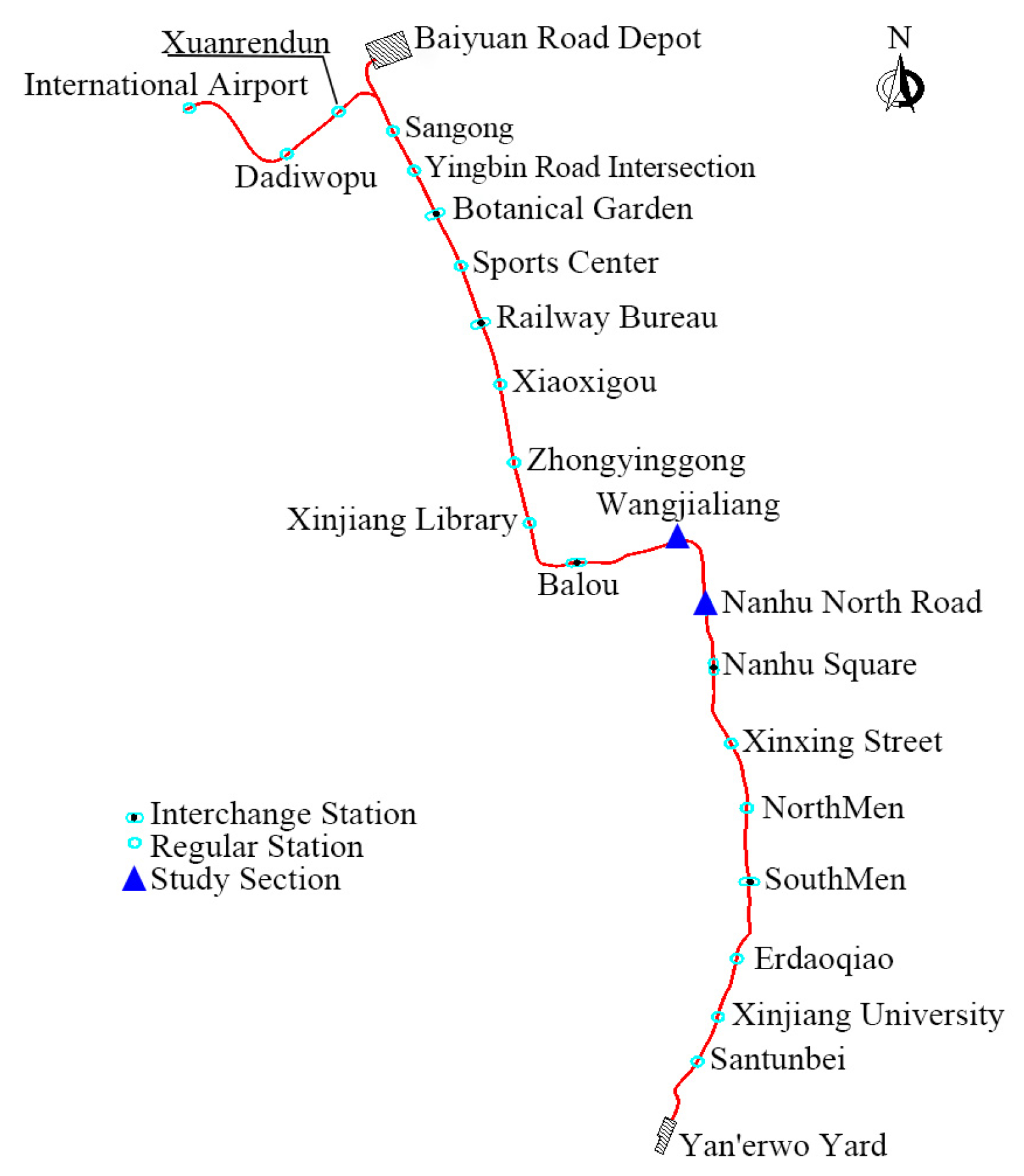
This study utilizes measured structural settlement data from the Nan-Wang section of Urumqi Metro Line 1 as a case study to validate the reliability and effectiveness of the proposed model. A schematic diagram of the metro line alignment is presented in Figure 2.

3.1. Project Overview

The Nan-Wang section was constructed using a combination of cut-and-cover and mining methods. The engineering geological conditions of the site are notably complex. The tunnel alignment primarily traverses strata composed of round gravel and cobblestone layers, which are typically characterized by high permeability and poor stability. The heterogeneity of these conditions is further exacerbated by the localized distribution of clayey silt and fine sand within the cobblestone layers. Moreover, the poor mechanical properties of the on-site rock formations present a risk of unexpected settlement deformation under the influence of construction disturbances and long-term operational loads, posing a potential threat to the structural integrity and long-term operational safety of the subway line. Therefore, monitoring the tunnel structure in this section and developing a high-precision prediction model based on the collected data are crucial for ensuring the safety of subway operations.

3.2. Deformation Monitoring Data

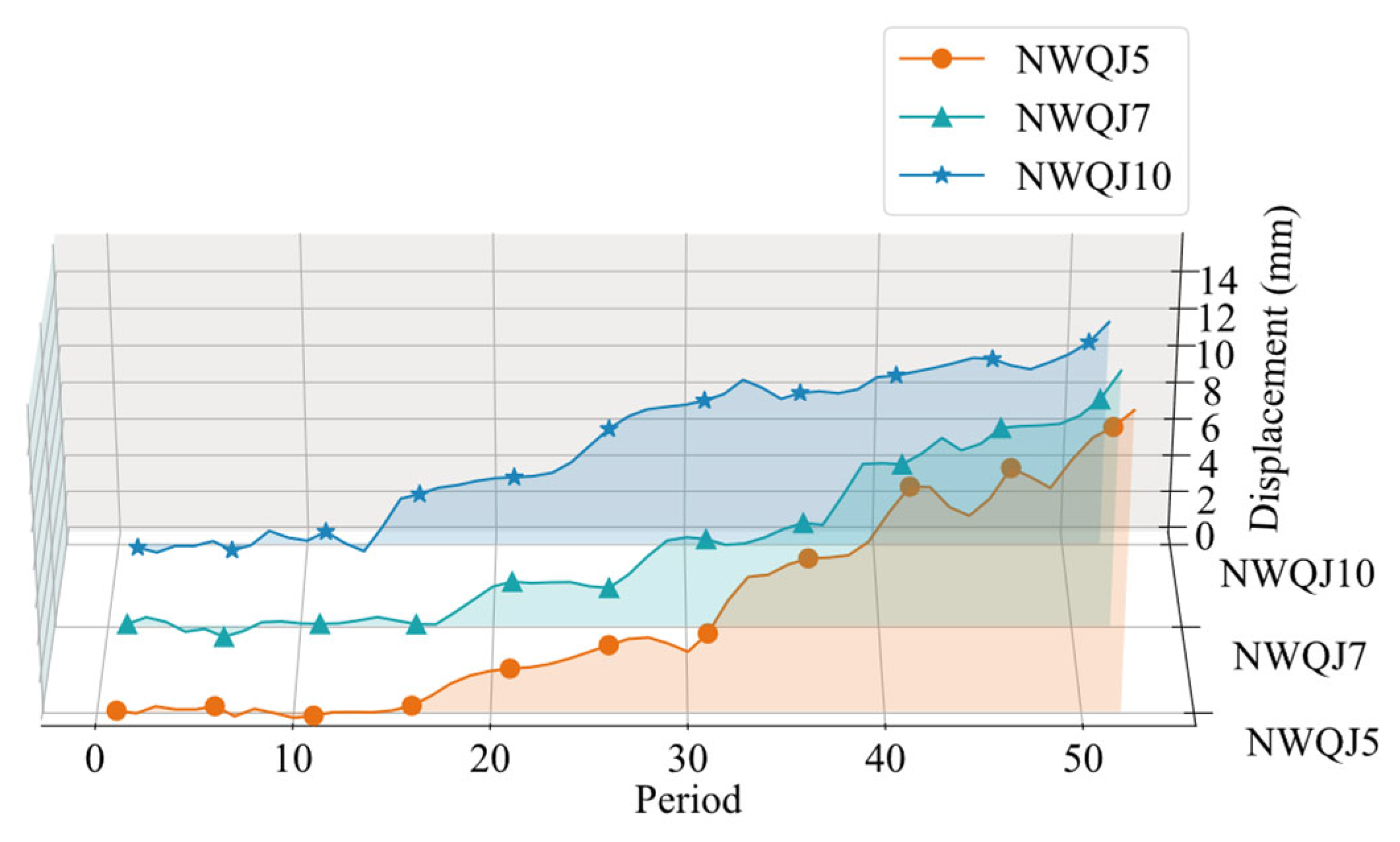
Monitoring the structural deformation of a tunnel is an essential method for understanding and tracking its structural changes, identifying potential hazards, and assessing its overall safety condition. Within the Nan-Wang section, 27 structural settlement monitoring points were installed, with data collected monthly over 52 months Trimble DINI 03 digital level (Trimble Inc., Westminster, CO, USA). For this study, NWQJ5, NWQJ7, and NWQJ10 were selected based on their high data integrity and diverse environmental representativeness (covering residential areas, commercial, and traffic, respectively). Table 1 presents a portion of the cumulative settlement data from these points.

3.3. Model Construction and Result Analysis

3.3.1. Data Pre-Processing

Monitoring of the tunnel commenced on 7 March 2019, and ended on 17 June 2023. However, due to factors such as instrumentation, observation conditions, and personnel, the monitoring intervals were not uniform. Such non-equidistant time series data is suboptimal for model construction and the precise capture of deformation trends. Therefore, to ensure the accuracy of model training, the raw settlement data was first subjected to an interpolation process. This study employed the Cubic Spline interpolation method to fill in missing values and transform the non-equidistant data into a standardized, equidistant dataset with a time step of 1 month. Specifically, the monitoring period index corresponds to the calendar month, where Period 1 represents March 2019 and Period 52 represents June 2023. All data pre-processing and subsequent experimental computations in this study were implemented using the Python 3.10 environment. Based on this processed sequence, the prediction task is defined as one-step-ahead rolling forecasting, thereby enabling the model to better capture the underlying deformation trends.
Considering that the raw monitoring data is inevitably contaminated by non-stationary high-frequency stochastic noise (often stemming from environmental vibrations and sensor precision limits), Wavelet Threshold Denoising was applied to extract the true deformation signal. To ensure the most effective noise removal, the wavelet basis function was not selected arbitrarily. Instead, a quantitative optimization strategy was implemented. We iterated through two major wavelet families: Daubechies (db1–db10) and Symlets (sym1–sym10). For each candidate basis, the Signal-to-Noise Ratio (SNR) and RMSE were calculated. The basis yielding the highest SNR and lowest RMSE was selected as the optimal choice for this specific dataset.
From an engineering interpretation standpoint, this specific denoising process is critical. It effectively filters out random high-frequency errors while strictly preserving the low-frequency structural settlement trends and medium-frequency seasonal fluctuations. This ensures that the input to the prediction model reflects the true mechanical deformation of the tunnel rather than sensor artifacts. Following this pre-processing, the dataset was partitioned into a 70% training set and a 30% test set to ensure the model’s robustness and generalization capability. The results of the data pre-processing are presented in Figure 3.

3.3.2. Comparison of Optimization Algorithms

To avoid the potential bias of selecting a single optimization method and to comprehensively investigate the impact of different algorithms on the performance of the GPR model, a comparative study was conducted. Five metaheuristic algorithms were selected for this comparison: the Whale Optimization Algorithm (WOA), Particle Swarm Optimization (PSO), Egret Swarm Optimization Algorithm (ESOA), Harris Hawks Optimization (HHA), and the proposed Hippopotamus Optimization (HO) algorithm.
To ensure a fair comparison, the population size for each algorithm was set to 10 and the maximum number of iterations was set to 30. All other parameters were configured based on established principles and common empirical values for each respective algorithm. The pre-processed data from monitoring point NWQJ5 was used for all comparative experiments. Given the stochastic nature of metaheuristic algorithms, each optimization was repeated 10 times, and the final evaluation was based on the average of the performance metrics obtained from these runs. The predictive performance evaluation results for the GPR model optimized by each algorithm are presented in Table 2.
The evaluation results demonstrate distinct differences in the effectiveness of various optimization algorithms for enhancing GPR model performance through hyperparameter tuning. Among the compared algorithms, the proposed HO-GPR model exhibited superior comprehensive performance. It achieved the highest coefficient of determination (R2) of 0.973, whereas the WOA yielded the lowest R2 of 0.937. Furthermore, the HO-GPR model consistently recorded the lowest values for RMSE, MAE, and MAPE among the five optimization algorithms tested. Driven by this empirical evidence, along with its theoretical advantage in balancing global exploration and local exploitation to avoid local optima, the HO algorithm was selected as the optimal optimizer for the GPR model in this study.
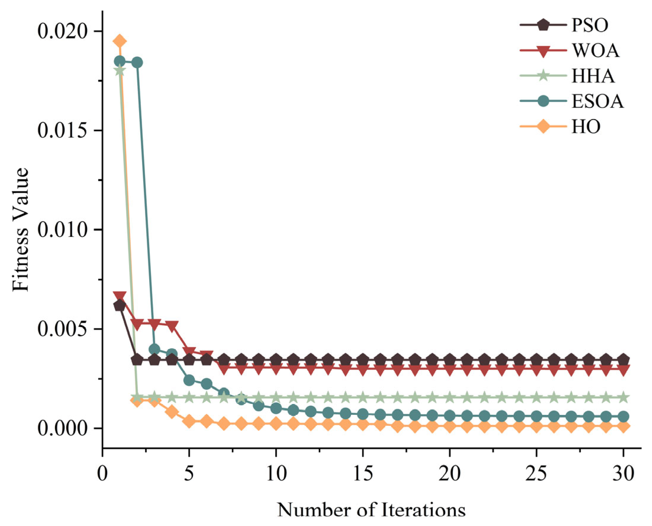
Figure 4 displays the fitness curves for each optimization algorithm. As shown, the PSO algorithm yielded the highest final fitness value and exhibited the slowest convergence. This is primarily attributed to its comparatively insufficient global search capability when addressing complex, non-linear problems of this nature, making it susceptible to convergence at local optima. The optimization performances of WOA, HHA, and ESOA were found to be broadly comparable, with similar values across the four evaluation metrics. In contrast, the HO algorithm showed the most effective convergence behavior, reaching the minimum fitness value at the 12th iteration. Therefore, by virtue of its powerful global exploration and local exploitation capabilities, the HO algorithm can more effectively perform the hyperparameter tuning task for the GPR model. This results in the construction of a prediction model with superior accuracy and robustness.

3.3.3. Comparative Analysis of Different Models

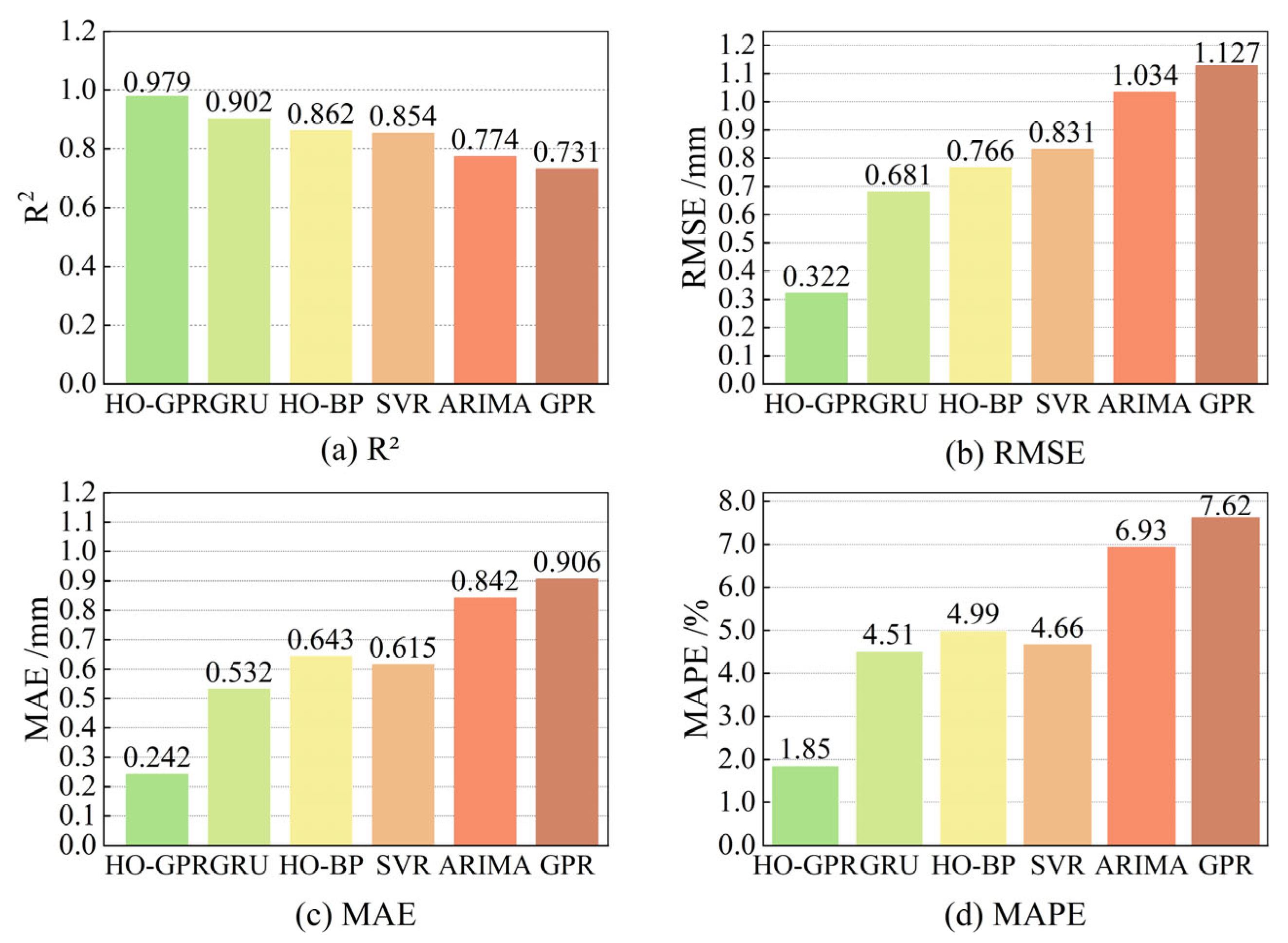
To validate the performance of the proposed HO-GPR model against other established prediction methods, a comparative analysis was conducted using the measured data from monitoring point NWQJ5. The selected benchmark models include a Gated Recurrent Unit (GRU) network, Support Vector Regression (SVR), a BP neural network optimized by the same algorithm (HO-BP), a standard GPR model, and a time series statistical model (ARIMA). The predictive performance metrics for all models are presented in Figure 5 and Table 3.
The results demonstrate that the proposed HO-GPR model consistently outperforms the other five models across all indicators. Specifically, the HO-GPR model achieved an R2 of 0.979, showing a significant improvement over the standalone standard GPR model (R2 = 0.731). In comparison, the R2 values for the GRU, HO-BP, SVR, and ARIMA models were 0.902, 0.862, 0.854, and 0.774, respectively. Furthermore, the HO-GPR model recorded the lowest error metrics, with an RMSE of 0.318 mm, an MAE of 0.240 mm, and a MAPE of 1.83%, all of which were substantially lower than those of the comparative models. Additionally, the statistical analysis in Table 3 confirms that these improvements are statistically significant (p < 0.001), with the 95% confidence intervals further demonstrating the stability of the proposed method.
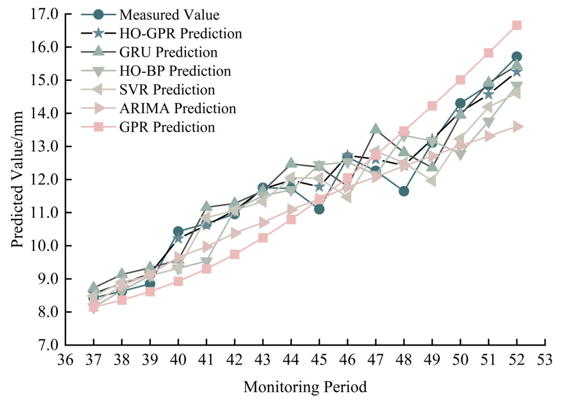
Figure 6 presents the comparison curves of the predicted and measured values for each model. It is evident that the standalone GPR and ARIMA models exhibit a distinct linear trend and perform poorly, struggling to effectively capture the complex non-linear characteristics of the settlement data. While the HO-BP and SVR models reflect the non-linear relationships to some extent, they show significant deviations from the measured values in segments with high data volatility, limiting their prediction accuracy. The GRU model, leveraging its recurrent structure and gating mechanisms, provides a better overall fit by capturing non-linear features more effectively. However, it still fails to fully track sharp fluctuations in the data, indicating a need for further improvement in its predictive precision. A critical instance occurs during periods 45–51, where a distinct peak in measured settlement is observed. From an engineering perspective, this phenomenon is attributed to the mechanical disturbance and the void between the tunnel segments and the surrounding soil, leading to rapid ground stress release and a sharp increase in settlement. Ordinary models typically struggle to predict such abrupt non-linear changes.
In contrast, the HO-GPR model demonstrates excellent adaptability to these complex engineering conditions. The settlement trend predicted by the HO-GPR model maintains a high degree of consistency with the measured results, demonstrating outstanding predictive performance. These results demonstrate that the proposed hybrid model holds a significant advantage in processing complex, non-linear subway tunnel settlement data, offering substantial improvements in predictive performance and providing more accurate and reliable forecasts.

3.3.4. Generalization Validation

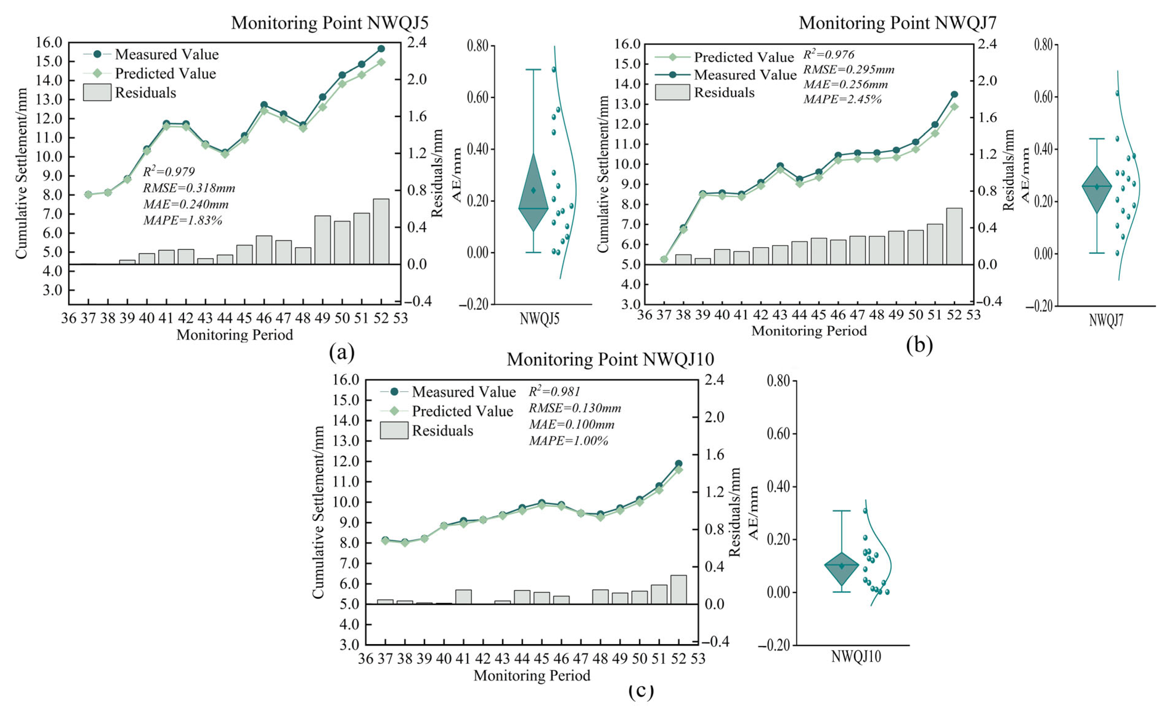
The generalization capability of the HO-GPR model was validated on three independent datasets from the aforementioned monitoring points (NWQJ5, NWQJ7, and NWQJ10). Specifically, the model was trained using data from NWQJ5 and subsequently applied without retraining to predict settlement at points NWQJ7 and NWQJ10. Figure 7 illustrates the comparison between the measured and predicted values, as well as the Absolute Error (AE), for each of the three monitoring points. The AE is calculated as A E = | M e a s u r e d   V a l u e P r e d i c t e d   V a l u e | .
The model exhibited superior fitting performance at monitoring point NWQJ10, recording the highest R2 of 0.981 alongside the lowest error metrics among all monitoring points, with an RMSE of 0.130 mm, an MAE of 0.100 mm, and a MAPE of 1.00%. Furthermore, the median Absolute Error (AE) for NWQJ10 was only 0.104 mm, indicating that the HO-GPR model successfully captured the intrinsic patterns of the settlement data with high precision. For monitoring points NWQJ5 and NWQJ7, the performance comparison reveals mixed results. Specifically, NWQJ5 achieved a slightly higher R2 of 0.979 compared to 0.976 for NWQJ7, suggesting a better fit for the overall trend. However, its RMSE was marginally higher at 0.318 mm compared to 0.295 mm for NWQJ7, implying the presence of larger outliers in the NWQJ5 predictions. Nevertheless, regarding overall accuracy metrics, NWQJ5 outperformed NWQJ7, yielding lower MAE and MAPE values of 0.240 mm and 1.83%, respectively, compared to 0.256 mm and 2.45% for NWQJ7. Notably, the median AE of NWQJ5 was 0.171 mm, significantly lower than the 0.259 mm observed at NWQJ7. This discrepancy is primarily attributed to the error distribution: although NWQJ5 exhibited accumulated errors in the final four monitoring periods—which elevated the RMSE—its prediction errors during the intermediate phase (periods 38–48) were consistently smaller than those of NWQJ7. Consequently, NWQJ5 demonstrated superior overall robustness despite the late-stage deviations.
Ultimately, despite slight performance variations attributable to the distinct characteristics of each dataset, the HO-GPR model consistently maintained high prediction accuracy and robustness across all tests. These results affirm the model’s excellent generalization capability and validate its effectiveness for practical applications.

4. Conclusions

This paper introduced the Hippopotamus Optimization (HO) algorithm to a Gaussian Process Regression (GPR) model to optimize its kernel function hyperparameters, resulting in the construction of a hybrid HO-GPR subway tunnel settlement prediction model. Based on measured data from the Nan-Wang section of Urumqi Metro Line 1, the study validated the performance enhancements offered by five different optimization algorithms and conducted a comparative analysis against five other prediction models. The main conclusions are as follows:
(1) The proposed HO-GPR model effectively overcomes the limitations of traditional optimization methods, which are prone to converging at local optima, by introducing the HO algorithm for global hyperparameter tuning. The results demonstrate that by leveraging the algorithm’s powerful global exploration and local exploitation capabilities, this approach significantly enhances the model’s prediction accuracy and generalization capability.
(2) Taking the typical monitoring point NWQJ5 as an example, the HO-GPR model significantly outperforms existing methods in accuracy and stability, achieving an R2 of 0.979, with RMSE, MAE, and MAPE values of 0.318 mm, 0.240 mm, and 1.83%, respectively. Compared to benchmarks (GRU, SVR, HO-BP, GPR, and ARIMA), it demonstrates an absolute R2 improvement of 0.077–0.248 and reduces prediction errors by 53.3–76.0%.
(3) The results of the generalization validation experiments confirmed that the model exhibits robust and effective predictive performance across different monitoring points, further proving its adaptability and generalization capability in complex tunnel environments.
In summary, the hybrid HO-GPR model can effectively address the non-linear and non-stationary challenges present in subway tunnel deformation monitoring data. Therefore, it can serve as a highly efficient tool for subway tunnel deformation forecasting.
In terms of practical engineering implementation, the proposed HO-GPR model demonstrates high computational efficiency, making it well-suited for integration into intelligent Structural Health Monitoring (SHM) systems. To handle real-time data streams and adapt to dynamic conditions during construction and operation, a sliding window-based dynamic updating strategy can be implemented. Specifically, as new monitoring data is acquired, the model’s training set is updated to include the most recent observations. The HO algorithm can then periodically re-optimize the GPR hyperparameters to capture evolving deformation characteristics and environmental influences. Furthermore, by embedding this predictive engine into existing tunnel monitoring software platforms, engineers can visualize future settlement trends alongside real-time sensor data. This integration allows for the establishment of an automated early warning mechanism, where alarms are triggered immediately if predicted values exceed safety control thresholds, thereby facilitating proactive risk management.
However, this study has certain limitations. The dataset used is relatively small, covering a limited monitoring duration, which may constrain the model’s ability to capture long-term seasonal variations and extreme deformation events. Furthermore, the model relies solely on historical settlement sequences as input, ignoring the potential influence of external physical factors such as geological strata conditions and groundwater levels. In future work, we plan to mitigate these issues by:
(1) Extending the monitoring duration and frequency to construct a larger-scale and higher-granularity dataset, thereby improving the model’s robustness.
(2) Adopting a multi-source data fusion strategy. Specifically, we aim to incorporate geological parameters and environmental factors as auxiliary input variables to further enhance the interpretability and generalization capability of the prediction model.

Author Contributions

Funding acquisition, J.C.; data analysis, writing—original draft, visualization, X.Y.; resources, writing—review and editing, W.D. All authors have read and agreed to the published version of the manuscript.

Funding

This research was supported by the National Natural Science Foundation of China (Grant No. 51868074); the Natural Science Foundation of Xinjiang Uygur Autonomous Region (Grant No. 2022D01C55); and the Key R&D Program of Xinjiang (Grant No. 2022B03033-1).

Data Availability Statement

The data are available upon request due to privacy/ethical restrictions.

Acknowledgments

We sincerely thank the anonymous reviewers for their insightful and constructive comments and suggestions on the earlier version of the manuscript.

Conflicts of Interest

The authors declare no conflicts of interest. The funders had no role in the design of the study; in the collection, analyses or interpretation of data; in the writing of the manuscript; or in the decision to publish the results.

References

  1. Huang, Y.; Fei, G. Deformation prediction model of metro based on GA-BP neural network. J. Hefei Univ. Technol. 2021, 44, 1513–1517. [Google Scholar] [CrossRef]
  2. Zhang, Y.; Di, H.; Xu, Y. Machine learning based prediction model for long-term settlement in a metro-shield tunnel. Urban Rapid Rail Transit 2022, 35, 89–94. [Google Scholar] [CrossRef]
  3. Hu, L.; Kasama, K.; Wang, G.; Takahashi, A. Assessing the influence of geotechnical uncertainty on existing tunnel settlement caused by new tunneling underneath. Tunn. Undergr. Space Technol. 2025, 155, 106189. [Google Scholar] [CrossRef]
  4. Zhang, B.Q.; Wang, S.H.; Zhang, Z.; Wang, P.Y.; Dong, F.R. Prediction method of tunnel deformation based on time series and DEGWO-SVR model. J. Northeast. Univ. 2021, 42, 2275–2285. [Google Scholar] [CrossRef]
  5. Fu, H.Y.; Zhao, Y.Y.; Ding, H.J.; Rao, Y.-K.; Yang, T.; Zhou, M.-Z. A novel intelligent displacement prediction model of karst tunnels. Sci. Rep. 2022, 12, 16983. [Google Scholar] [CrossRef]
  6. Feng, X.; Jiang, J.; Bao, W.; Ma, X.; Liu, H. Research on predicting structural deformation of subway tunnels induced by foundation pit construction integrating spatiotemporal features. J. Railw. Sci. Eng. 2025, 22, 3592–3603. [Google Scholar] [CrossRef]
  7. He, Y.; Guo, J.; Liu, H. Application of Time Series Analysis Model in Subway Tunnel Settlement Deformation Monitoring. Geomat. Spat. Inf. Technol. 2022, 45, 238–240. [Google Scholar] [CrossRef]
  8. Wang, S.; Yu, R.; Dong, F.; Wang, Y.; Zhang, H.; Liu, K. Prediction of Settlement of Shield Tunnel Subway Tunnel Roof Based on WOA-BP Neural Network. J. Basic Sci. Eng. 2025, 33, 770–778. [Google Scholar] [CrossRef]
  9. Zhang, Q.; Ma, Y.; Zhang, B.; Tian, L.; Zhang, G. Time Series Prediction on Settlement of Metro Tunnels Adjacent to Deep Foundation Pit by Clustering Monitoring Data. KSCE J. Civ. Eng. 2023, 27, 2180–2190. [Google Scholar] [CrossRef]
  10. Li, C.; Li, J.; Shi, Z.; Li, L.; Li, M.; Jin, D.; Dong, G. Prediction of Surface Settlement Induced by Large-Diameter Shield Tunneling Based on Machine-Learning Algorithms. Geofluids 2022, 2022, 4174768. [Google Scholar] [CrossRef]
  11. Saleti, S.; Panchumarthi, L.Y.; Kallam, Y.R.; Parchuri, L.; Jitte, S. Enhancing Forecasting Accuracy with a Moving Average-Integrated Hybrid ARIMA-LSTM Model. SN Comput. Sci. 2024, 5, 704. [Google Scholar] [CrossRef]
  12. Zhang, M.; Qin, S.; Li, P.; Ge, C.; Yang, M.; Xie, Z. Deep excavation deformation prediction method based on BP Neural Network with integrated attention mechanism. J. Beijing Jiaotong Univ. 2025, 49, 95–104. [Google Scholar]
  13. Lai, J.; Zhu, J.; Guo, Y.; Xie, Y.; Hu, Y.; Wang, P. A multi-factor-driven approach for predicting surface settlement caused by the construction of subway tunnels by undercutting method. Environ. Earth Sci. 2024, 83, 442. [Google Scholar] [CrossRef]
  14. Latif, K.; Sharafat, A.; Seo, J. Digital Twin-Driven Framework for TBM Performance Prediction, Visualization, and Monitoring through Machine Learning. Appl. Sci. 2023, 13, 11435. [Google Scholar] [CrossRef]
  15. Sharafat, A.; Latif, K.; Seo, J. Risk analysis of TBM tunneling projects based on generic bow-tie risk analysis approach in difficult ground conditions. Tunn. Undergr. Space Technol. 2021, 111, 103860. [Google Scholar] [CrossRef]
  16. Zhang, P.; Wu, H.-N.; Chen, R.-P.; Chan, T.H. Hybrid meta-heuristic and machine learning algorithms for tunneling-induced settlement prediction: A comparative study. Tunn. Undergr. Space Technol. 2020, 99, 103383. [Google Scholar] [CrossRef]
  17. Lan, T.; Zhou, Y.; Sun, X.; Wang, J.; Lu, L. Adaptive Deformation Feature Analysis Based on Gaussian Process Regression and Its Application. Sci. Surv. Mapp. 2024, 49, 21–28. [Google Scholar] [CrossRef]
  18. Liu, D.X.; Zhou, Y. A Prediction Method of Ground Deformation in Subway Tunnel Construction based on Gaussian Process Regression. In Proceedings of the 2020 IEEE International Conference on Industrial Application of Artificial Intelligence (IAAI), Harbin, China, 25–27 December 2020. [Google Scholar] [CrossRef]
  19. Zheng, S.; Jiang, A.N.; Yang, X.R. Tunnel displacement prediction under spatial effect based on Gaussian process regression optimized by differential evolution. Neural Netw. World 2021, 31, 211–226. [Google Scholar] [CrossRef]
  20. Xia, H.Y. Application of Gaussian Process Machine Learning in Deformation Prediction of Foundation Pit of Subway Station Near River. Hebei J. Ind. Sci. Technol. 2022, 39, 364–372. [Google Scholar] [CrossRef]
  21. Zhang, F.; Su, Q.; Deng, Z.; Wang, C.; Cui, M.; Zhou, C. Research on Deformation Prediction and Application of Subway Station Foundation Pit Based on GF-GPR. J. Hefei Univ. Technol. 2025, 48, 563–569. [Google Scholar] [CrossRef]
  22. Liu, Z.; Lyu, C.; Huo, J.; Wang, S.; Chen, J. Gaussian Process Regression for Transportation System Estimation and Prediction Problems: The Deformation and a Hat Kernel. IEEE Trans. Intell. Transp. Syst. 2022, 23, 22331–22342. [Google Scholar] [CrossRef]
  23. Amiri, M.H.; Mehrabi Hashjin, N.; Montazeri, M.; Mirjalili, S.; Khodadadi, N. Hippopotamus optimization algorithm: A novel nature-inspired optimization algorithm. Sci. Rep. 2024, 14, 5032. [Google Scholar] [CrossRef]
  24. Mura, R.; Floris, G.; Scionis, L.; Piras, G.; Pintor, M.; Demontis, A.; Giacinto, G.; Biggio, B.; Roli, F. HO-FMN: Hyperparameter optimization for fast minimum-norm attacks. Neurocomputing 2025, 616, 128918. [Google Scholar] [CrossRef]
  25. Liu, Y.; Peng, J.; Ren, L.; Gao, B.; Guo, J.; Wang, Z.; Han, H. Forecasting of Horizontal Deformation in Retaining Piles of Subway Station Deep Foundation Pits Based on the CEEMDAN-SSA-ELM-LSTM Model. J. Disaster Prev. Mitig. Eng. 2025. [Google Scholar] [CrossRef]
  26. Qiu, P.; Liu, F.; Zhang, J. Land Subsidence Prediction Model Based on the Long Short-Term Memory Neural Network Optimized Using the Sparrow Search Algorithm. Appl. Sci. 2023, 13, 11156. [Google Scholar] [CrossRef]
  27. Zhang, W.-S.; Yuan, Y.; Long, M.; Yao, R.-H.; Jia, L.; Liu, M. Prediction of surface settlement around subway foundation pits based on spatiotemporal characteristics and deep learning models. Comput. Geotech. 2024, 168, 106149. [Google Scholar] [CrossRef]
  28. Zhu, S.; Qin, Y.; Meng, X.; Xie, L.; Zhang, Y.; Yuan, Y. Prediction model of land surface settlement deformation based on improved LSTM method: CEEMDAN-ICA-AM-LSTM (CIAL) prediction model. PLoS ONE 2024, 19, e0298524. [Google Scholar] [CrossRef]
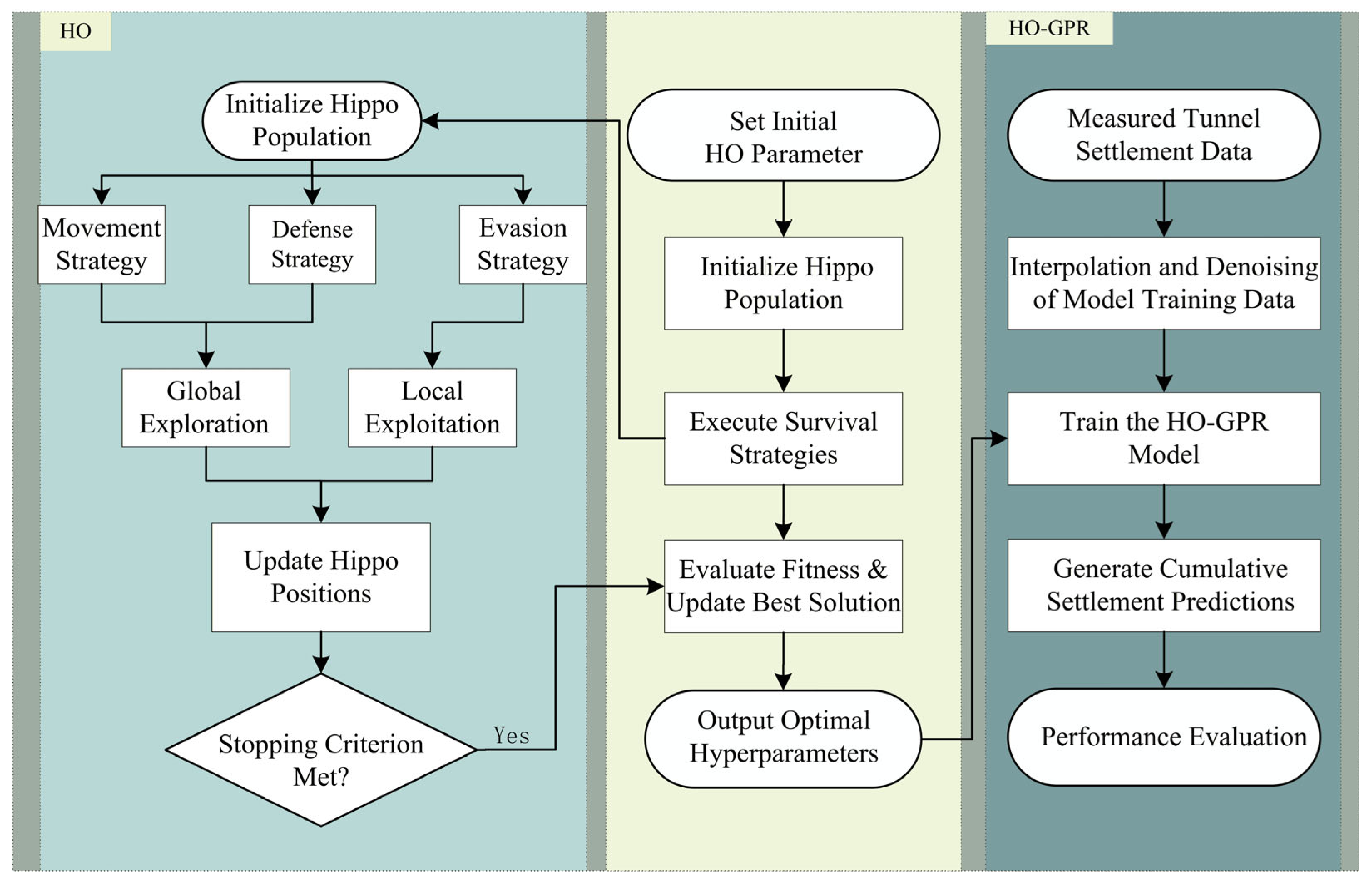
Figure 1. Framework of the GPR-based settlement prediction model optimized by the HO algorithm.
Buildings 16 00192 g001
Figure 2. Urumqi Metro Line Map.
Buildings 16 00192 g002
Figure 3. Time series of the final preprocessed settlement data for monitoring points NWQJ5, NWQJ7, and NWQJ10.
Buildings 16 00192 g003
Figure 4. Convergence Curve.
Buildings 16 00192 g004
Figure 5. Comparison of evaluation metrics for the different models.
Buildings 16 00192 g005
Figure 6. Comparison between predicted settlement results and measured values for each model.
Buildings 16 00192 g006
Figure 7. Settlement Prediction Results of the HO-GPR Model. (a) Monitoring Point NWQJ5; (b) Monitoring Point NWQJ7; (c) Monitoring Point NWQJ10. The green plots on the right side of each subfigure illustrate the distribution of the Absolute Errors (AE).
Buildings 16 00192 g007
Table 1. Monitored structural settlement data.
PeriodDateCumulative Settlement/mm
NWQJ5NWQJ7NWQJ10
1March 2019−0.18−0.2−0.49
2April 2019−0.370.2−0.78
3May 20190.020.0−0.42
50April 202314.3011.929.30
51May 202314.8511.9810.80
52June 202315.7113.4911.90
Table 2. Performance Comparison of Different Optimization Algorithms.
Optimization AlgorithmR2RMSE/mmMAE/mmMAPE
WOA0.9370.4690.3792.95%
PSO0.9590.3890.3182.51%
HHA0.9670.3710.3022.36%
ESOA0.9680.3640.2952.42%
HO0.9730.3310.2642.03%
Table 3. Statistical comparison of prediction performance on the NWQJ5 dataset. Values are reported as the bootstrap mean (95% confidence interval) over 2000 replicates.
Prediction ModelR2 (95% CI)p-ValueRMSE (95% CI)p-Value
HO-GPR0.976 (0.951–0.987)-0.317 (0.205–0.433)-
GRU0.885 (0.741–0.958)<0.0010.674 (0.431–0.899)<0.001
HO-BP0.853 (0.657–0.944)<0.0010.756 (0.581–0.922)<0.001
SVR0.839 (0.676–0.918)<0.0010.816 (0.519–1.129)<0.001
ARIMA0.747 (0.492–0.874)<0.0011.015 (0.717–1.310)<0.001
GPR0.674 (0.175–0.902)<0.0011.109 (0.731–1.454)<0.001
Note: p-value indicate statistical significance compared to the HO-GPR model. Minor deviations from Figure 5 are due to the bootstrap resampling process.
Disclaimer/Publisher’s Note: The statements, opinions and data contained in all publications are solely those of the individual author(s) and contributor(s) and not of MDPI and/or the editor(s). MDPI and/or the editor(s) disclaim responsibility for any injury to people or property resulting from any ideas, methods, instructions or products referred to in the content.