Abstract
Buildings account for nearly 32% of global energy consumption and serve as key demand-side flexibility resources in power systems with high renewable penetration. However, their utilization is constrained by the lack of an integrated framework that can jointly quantify energy-adjustable margin (BAM) and response duration (RD) under realistic operational and thermal comfort constraints. This study presents a coupled data–physical simulation framework integrating a Particle Swarm Optimization–Long Short-Term Memory–Random Forest (PSO-LSTM-RF) hybrid load forecasting model with EnergyPlus(24.1.0)-based building simulation. The PSO-LSTM-RF model achieves high-accuracy short-term load prediction, with an average R2 of 0.985 and mean absolute percentage errors of 1.92–5.75%. Predicted load profiles are mapped to physically consistent baseline and demand-response scenarios using a similar-day matching mechanism, enabling joint quantification of BAM and RD under explicit thermal comfort constraints. Case studies on offices, shopping malls, and hotels reveal significant heterogeneity: hotels exhibit the largest BAM (up to 579.27 kWh) and longest RD (up to 135 min), shopping malls maintain stable high flexibility, and offices show moderate BAM with minimal operational disruption. The framework establishes a closed-loop link between data-driven prediction and physics-based simulation, providing interpretable flexibility indicators to support demand-response planning, virtual power plant aggregation, and coordinated optimization of source–grid–load interactions.
1. Introduction
1.1. Research Background
Amid the escalating global energy crisis and climate change challenges, building energy conservation has become a critical component for achieving sustainable development. Buildings account for a substantial share of global energy consumption. According to the Global Status Report for Buildings 2024–2025 published by the United Nations Environment Programme (UNEP) [1], the building sector consumes approximately 32% of the world’s total energy. In China, rapid urbanization and rising living standards have driven a continuous increase in building energy consumption, making buildings a central target for energy-saving measures and demand-side flexibility exploitation.
Meanwhile, the development of modern power systems has facilitated the large-scale integration of high shares of renewable energy [2]. The intermittent and volatile nature of these energy sources poses significant challenges to grid supply–demand balancing [3]. Against this backdrop, buildings, as key flexible load resources within the power system, possess building adjustable margin (BAM)—the additional capacity for energy adjustment without compromising normal operations—which serves as a crucial link for coordinated optimization between building energy systems and the power grid. Notably, the quantification of BAM is not an unconstrained reduction in energy consumption; instead, it must adhere to the rigid bottom line of maintaining thermal comfort, a core requirement for buildings to fulfill their intended functions. As corroborated by Khatoon and Shah [4] in their study on naturally ventilated underground car parks, the accurate prediction of thermal comfort parameters is a prerequisite for effective energy optimization, and any adjustment space divorced from thermal comfort constraints will lose practical application value. To fully characterize building flexibility in supporting grid scheduling, it is necessary to simultaneously assess BAM and response duration (RD)—defined as the time interval from the start of air-conditioning shutdown (for demand response) to system restart (triggered by indoor temperature reaching the upper comfort threshold of 28 °C). Accurate forecasting and assessment of both BAM and RD can guide buildings to participate in demand-response programs more effectively: BAM quantifies the maximum load adjustment potential, while RD clarifies the sustainable duration of this adjustment, jointly supporting peak shaving and valley filling in the grid. This approach not only enhances the integration of renewable energy but also reduces building energy costs, achieving a dual benefit for both the grid and building operators.
However, systematic assessment and predictive research on BAM and RD remain limited. This gap often leads to discrepancies between declared and actual response capacities when buildings participate in demand response. Existing studies primarily focus on macro-level quantification of flexibility potential or demand-response capacity, and have yet to establish a dedicated methodology for assessing BAM together with RD. Specifically, two core limitations can be identified: First, there is a bias in the assessment perspective. Most current studies emphasize load-shifting potential for individual buildings and quantify load adjustment capacity but do not couple BAM (energy dimension) with RD (temporal dimension) as a dedicated evaluation metric. Consequently, these studies are insufficient to meet the grid’s requirement for dual-dimensional (energy-time) load scheduling. Second, there is a disruption in the technical chain. Existing research either relies on simulation tools to generate potential data without precise predictive support or focuses on predictive model development without forming a closed-loop framework with BAM and RD quantification. To date, a complete technical chain integrating load forecasting, scenario simulation, and BAM-RD quantification has not been established.
In this context, the demand for demand-side flexibility of buildings in modern power systems is increasingly urgent. Motivated by this practical need, for the first time, this study proposes an integrated predictive framework integrating Particle Swarm Optimization (PSO), Long Short-Term Memory (LSTM), and Random Forest (RF) models with EnergyPlus(24.1.0) simulation technology. This framework specifically focuses on the precise quantification of BAM and RD, aiming to fill the current research gap and provide both theoretical support and practical pathways for public buildings to actively participate in modern power system interactions and enhance energy efficiency.
1.2. Research Status and Existing Problems
1.2.1. Current Status of Building Load Forecasting Research
Building load forecasting constitutes the foundation for energy margin assessment. In recent years, alongside the advancement of artificial intelligence technologies, significant progress has been achieved in forecasting methods for building loads. Currently, the commonly used forecasting methods mainly include traditional statistical methods, machine learning methods, and deep learning methods.
Among traditional statistical methods, Tarsitano [5] adopted a dynamic regression model that integrates key external predictive factors into the seasonal autoregressive integrated moving average process, achieving high accuracy in both one-day and nine-day forecasts. Huang [6] proposed combining sensor networks with Gaussian regression for building load forecasting and compared Gaussian process regression models using different covariance functions to determine the optimal one. These methods are conceptually simple and computationally efficient but show poor adaptability to nonlinear and nonstationary building load data. Within the classical framework of data dimensionality reduction in traditional statistical methods, the “similar day” approach—centered on the core assumption that “load patterns from historically similar scenarios can be transferred to the forecast day”—has been widely applied in building load forecasting. Its academic consensus and contentious focal points provide a design basis for the similar day selection model in this study. Currently, this method faces three core controversies: the first is the controversy over feature vector construction: single meteorological factors fail to capture the coupling effects of multiple factors, necessitating a balance between feature comprehensiveness and computational efficiency [7]; the second is the controversy over similarity calculation and weight setting: methods such as Euclidean distance and gray relational analysis have been adopted, yet weight configurations mostly rely on experience, leading to strong subjectivity [8]; the third is the limitation in applicability to complex scenarios: under scenarios like holidays or abrupt weather changes, multifactor coupling complicates load patterns, resulting in scarce similar samples and increased prediction errors in traditional methods [9]. To address the above controversies, this study optimizes the similar day selection logic from three aspects (indicator system, weight configuration, and scenario adaptability) to enhance the reliability of selection results.
In the research on load forecasting based on machine learning, scholars have gradually improved prediction accuracy and adaptability across different scenarios through algorithmic optimization. As an early core technical framework, the artificial neural network (ANN) established a foundational paradigm for subsequent load forecasting models. In recent years, researchers have innovated its application in data-scarce environments. Li [10] combined ANN with transfer learning algorithms to effectively address the challenge of insufficient training samples in data-driven models. The backpropagation (BP) neural network, as a classical implementation of ANN, has also been widely applied. Wang [11] used a BP neural network for power load prediction and analysis, improving the stability of forecasting results. Soon after, support vector machine (SVM) models were introduced into load forecasting. Luo [12] combined SVM with optimization algorithms, enhancing prediction accuracy while simplifying computation. Tang [13] developed a support vector regression (SVR) model for three power demand control scenarios, reducing model development time and labor cost. Wang [14] proposed a Random Forest (RF)-based model for predicting hourly electricity demand in buildings, while Sala [15] integrated RF with the K-means clustering algorithm for load forecasting in residential buildings.
As a branch of machine learning, deep learning models offer more network layers, enabling them to extract richer information from periodic energy consumption data [16]. Recurrent neural networks (RNNs) can capture valuable information from past sequences. Fang [17] proposed an improved singular spectrum analysis and multivariate input RNN, integrating multiple features from raw building electricity consumption time series data in Morocco. Rahman [18] developed an RNN-based method for predicting building electricity consumption, which significantly enhanced prediction accuracy by capturing time series characteristics and provided an efficient tool for energy management in commercial and residential buildings. However, RNNs often suffer from gradient vanishing or exploding issues when handling long sequences, making it difficult to effectively capture long-term dependencies [19]. To address this limitation, the Long Short-Term Memory (LSTM) network was introduced to capture temporal dependencies between sequences [20]. Zhou [21] applied an LSTM model to predict the time series of a university library’s air-conditioning system and demonstrated superior performance in energy consumption forecasting. Sundaram [22] employed LSTM for early prediction of residential electricity consumption, assisting in identifying energy efficiency improvement measures during early design stages. The temporal characteristics of energy consumption data greatly benefit from the LSTM model’s ability to capture time-based patterns and trends [23]. A review of the existing literature on deep learning methods shows that the LSTM model is widely used due to its capability to process sequential data, capture long-term correlations, manage missing data, and model complex interactions [24]. Therefore, the LSTM model is considered the optimal choice for load forecasting based on time series data.
However, building energy consumption data are influenced by multiple factors, such as temporal and meteorological characteristics. A single forecasting model cannot achieve both accuracy and efficiency in this context. Therefore, this study proposes a PSO-LSTM-RF hybrid model that overcomes the limitations of a single architecture. The PSO algorithm provides global optimization, alleviating computational redundancy and overfitting risk; RF, leveraging the advantages of ensemble learning, strengthens the capture of nonlinear coupling relationships among multidimensional features such as weather and time, compensating for the LSTM’s limitations in modeling nontemporal interactions. Together, the three models form a closed loop of “temporal dependency capture–multifeature integration–adaptive parameter optimization”, retaining the LSTM’s core advantage in handling long sequences while enhancing adaptability to complex building energy characteristics through cross-model collaboration, ultimately achieving high-accuracy and low-redundancy load forecasting.
1.2.2. Current Status of Building Adjustable Margin (BAM) Assessment Research
With the transformation of modern power systems toward high renewable energy penetration and power-electronic-dominated operation, electricity market mechanisms are evolving from traditional generation-load balancing to coordinated interaction among generation, grid, load, and storage. As a major flexible resource on the demand side, public buildings play a key role in ensuring the secure and economic operation of power systems through precise utilization of their energy regulation capacity [25,26]. Heating, ventilation, and air-conditioning (HVAC) systems are the core components in this regard, accounting for 40.00–60.00% of total building energy consumption [27,28]. The load characteristics and operating patterns of HVAC systems directly determine the potential boundaries of building energy regulation. On one hand, system start–stop operations and temperature setpoint adjustments can rapidly alter energy consumption levels, forming short-term load adjustment potential. On the other hand, the coupling with a building’s passive thermal storage capacity extends the duration of adjustment, providing more stable support for grid response. Therefore, prior forecasting of building flexibility is essential for participation in electricity markets. Whether for bidding in day-ahead markets, providing ancillary services in real-time markets, or enabling precise demand-response participation, buildings must determine in advance their BAM and RD.
The concept of BAM proposed in this study focuses on quantifying a building’s capacity to regulate energy in both the energy and temporal dimensions—a metric not yet explicitly defined in the current research context. To consolidate existing research and clarify the foundational understanding in this domain, related studies are reviewed using widely adopted terms such as building flexibility and demand-response potential. Yin [29] constructed detailed models of commercial and multifamily residential buildings using EnergyPlus(24.1.0), generating over 300 million data points to capture load response and thermodynamic characteristics, and fitted regression models incorporating time period, temperature setpoints, and outdoor temperature. Ding [30] adjusted indoor temperature setpoints and introduced two indicators—electrical flexibility and energy flexibility—to compare the performance of active storage, passive storage, and temperature reset strategies in demand-response processes. Ruan [31] analyzed how demand-response event types, thermal properties of building envelopes, and meteorological conditions affect preheating performance during the heating season, evaluating energy flexibility from the perspectives of energy efficiency, load reduction, and energy savings in a residential building in Kitakyushu, Japan. Han [32] proposed a probabilistic model using sampling-based fuzzy analysis to account for major uncertainties, enabling rapid quantification of aggregated flexibility in building clusters under uncertain conditions. Zhu [33] performed large-scale stochastic simulations for two common demand-response strategies, quantifying demand-response potential using metrics such as maximum response duration and maximum power reduction.
However, several limitations remain evident. First, most flexibility assessment studies rely on predefined or historical load profiles and lack predictive support that reflects future operating conditions. Second, flexibility is often quantified either in the energy dimension or the temporal dimension, rather than through a joint evaluation of adjustable margin and response duration. Third, the coupling between data-driven load forecasting and physics-based flexibility assessment has not been fully established, leading to fragmented technical chains and limited practical applicability.
To clearly distinguish existing studies from the proposed approach, a comparative analysis is presented in Table 1, which summarizes representative research from the perspectives of load forecasting, flexibility evaluation methods, and flexibility dimensions.

Table 1.
Comparison of existing studies and the proposed framework.
As shown in Table 1, existing studies have achieved notable progress in either high-accuracy load forecasting or detailed flexibility assessment using physical simulation. Nevertheless, these two research streams largely evolve independently. Load forecasting studies typically emphasize prediction performance without linking forecast results to executable flexibility indicators, while flexibility assessment studies often neglect predictive consistency with future operating scenarios.
Motivated by these limitations, this study proposes an integrated framework that couples data-driven load prediction with physics-based simulation through a similar-day matching mechanism, enabling the joint and realistic quantification of building adjustable margin and response duration. The main innovations and contributions of this study are summarized as follows:
- A closed-loop framework integrating load prediction and flexibility quantification is developed. Unlike existing studies that separately address building load forecasting or flexibility assessment, this study establishes an integrated technical chain that links high-accuracy data-driven load prediction with physics-based EnergyPlus simulation. By coupling prediction, similar-day matching, scenario construction, and margin calculation, the proposed framework resolves the long-standing disconnect between forecast results and practically executable flexibility indicators.
- A joint and physically constrained quantification of building adjustable margin and response duration is proposed. This study explicitly defines and quantifies BAM and RD as complementary indicators in the energy and temporal dimensions, under strict indoor thermal comfort constraints. By embedding comfort limits directly into the simulation-based evaluation process, the proposed method moves beyond abstract flexibility potential and provides practically feasible flexibility boundaries for demand-response applications.
- Building-type-dependent flexibility characteristics are systematically revealed through real-world case studies. Comparative analyses of office buildings, shopping malls, and hotels demonstrate distinct BAM–RD patterns across demand-response scenarios. The results provide actionable insights for selecting optimal response strategies for different building functions, supporting refined demand-response planning and the aggregation of heterogeneous building resources in virtual power plants.
2. Methodology
2.1. Methodological Framework
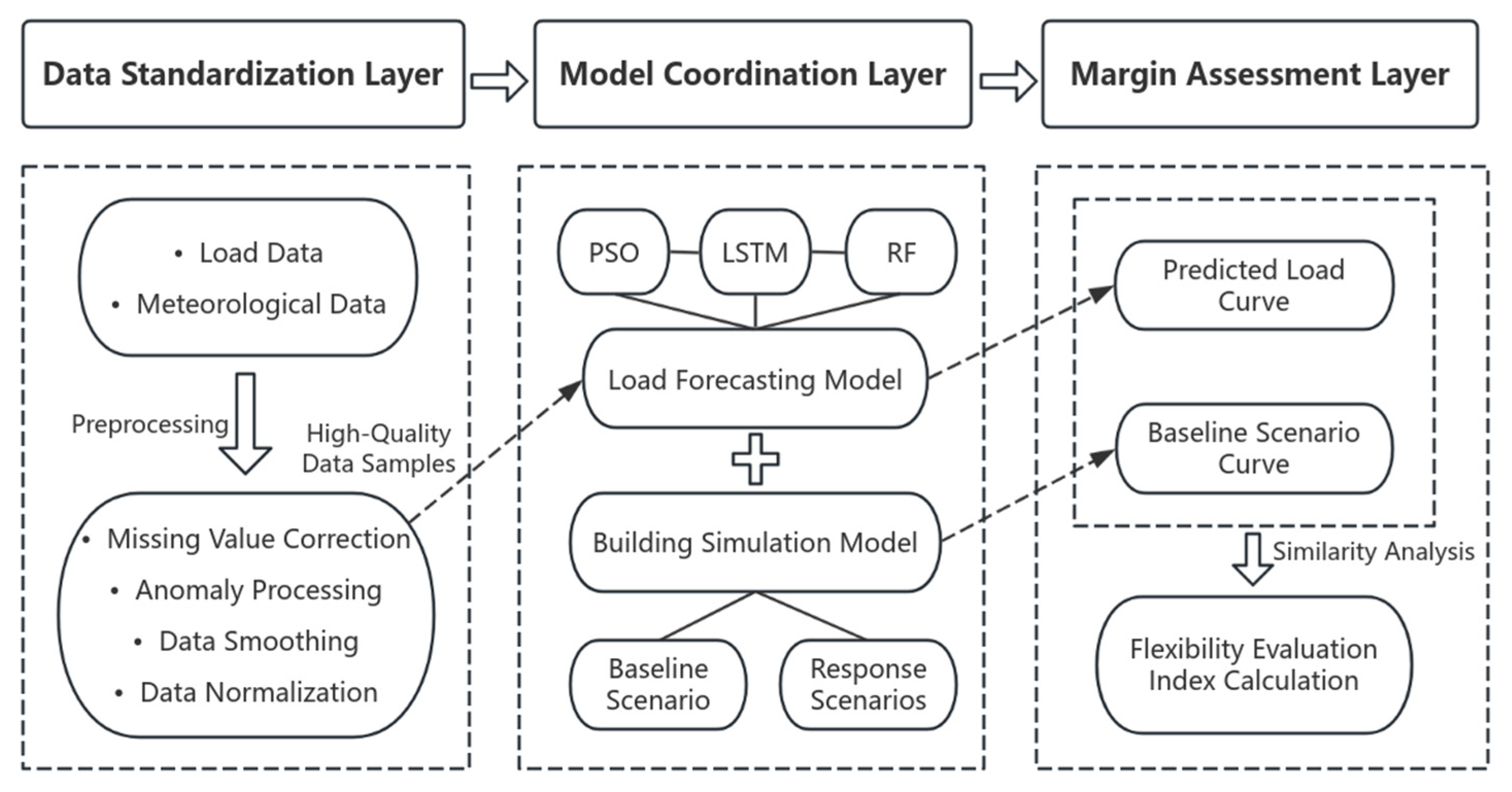
This study aims to achieve precise quantification of real energy margins for typical buildings under multiple scenarios. To this end, a three-tier methodological framework—comprising the data standardization layer, model coordination layer, and margin assessment layer—is established (Figure 1), forming a closed-loop process from data input, model computation, scenario simulation, to result output.
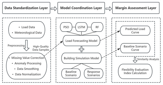
Figure 1.
Methodological framework diagram.
Existing studies have presented combined schemes of “machine learning prediction and EnergyPlus simulation”, but this framework differs in two core aspects (aligned with the three-tier structure in Figure 1):
- Scenario-adaptive hyperparameter optimization in the model coordination layer
Conventional schemes rely on fixed hyperparameters for machine learning models, which fail to accommodate the distinct load characteristics of different building types (e.g., offices, hotels) and weather conditions. In this framework, the PSO-LSTM-RF module (located in the model coordination layer) leverages PSO to dynamically tune LSTM/RF hyperparameters for each specific scenario. This adaptive adjustment enables the model to better capture scenario-specific load patterns, addressing the limitations of static parameter configurations in existing works.
- 2.
- Hierarchical cross-layer coupling of data-driven prediction and physical simulation (core workflow of the framework)
Most prior works only use EnergyPlus to generate static load datasets for model training, with no deep integration between predictive outputs and simulation processes. By contrast, this framework implements a sequential, four-stage cross-layer coupling:
- Stage 1 (Data Input and Prediction): The PSO-LSTM-RF module (model coordination layer) extracts high-dimensional temporal dependencies from standardized data (data standardization layer) to predict future building loads.
- Stage 2 (Baseline and Scenario Construction): The EnergyPlus model (model coordination layer) constructs a baseline scenario and four response scenarios (S1~S4) using real physical parameters of the building, generating energy consumption curves under different operation strategies.
- Stage 3 (Similar-Day Matching): The predicted load curve is compared with the baseline scenario curve via similarity analysis (margin assessment layer), solely to identify the most similar historical operating day (i.e., “similar day”) corresponding to the predicted load pattern.
- Stage 4 (Margin Calculation): Based on the identified similar day, EnergyPlus simulates the response scenarios, and the margin assessment layer derives the BAM and RD (the core outputs of this study).
This hierarchical, four-stage coupling represents a new paradigm of “data-driven prediction + physical simulation”: it first uses data models to capture future load trends, then identifies similar historical operating days to anchor the analysis to real building conditions, and finally leverages physics-based simulation to output practical flexibility indicators. This targeted integration addresses the disconnect between predictive models and actual building operations in conventional schemes.
2.2. PSO-LSTM-RF Hybrid Prediction Model
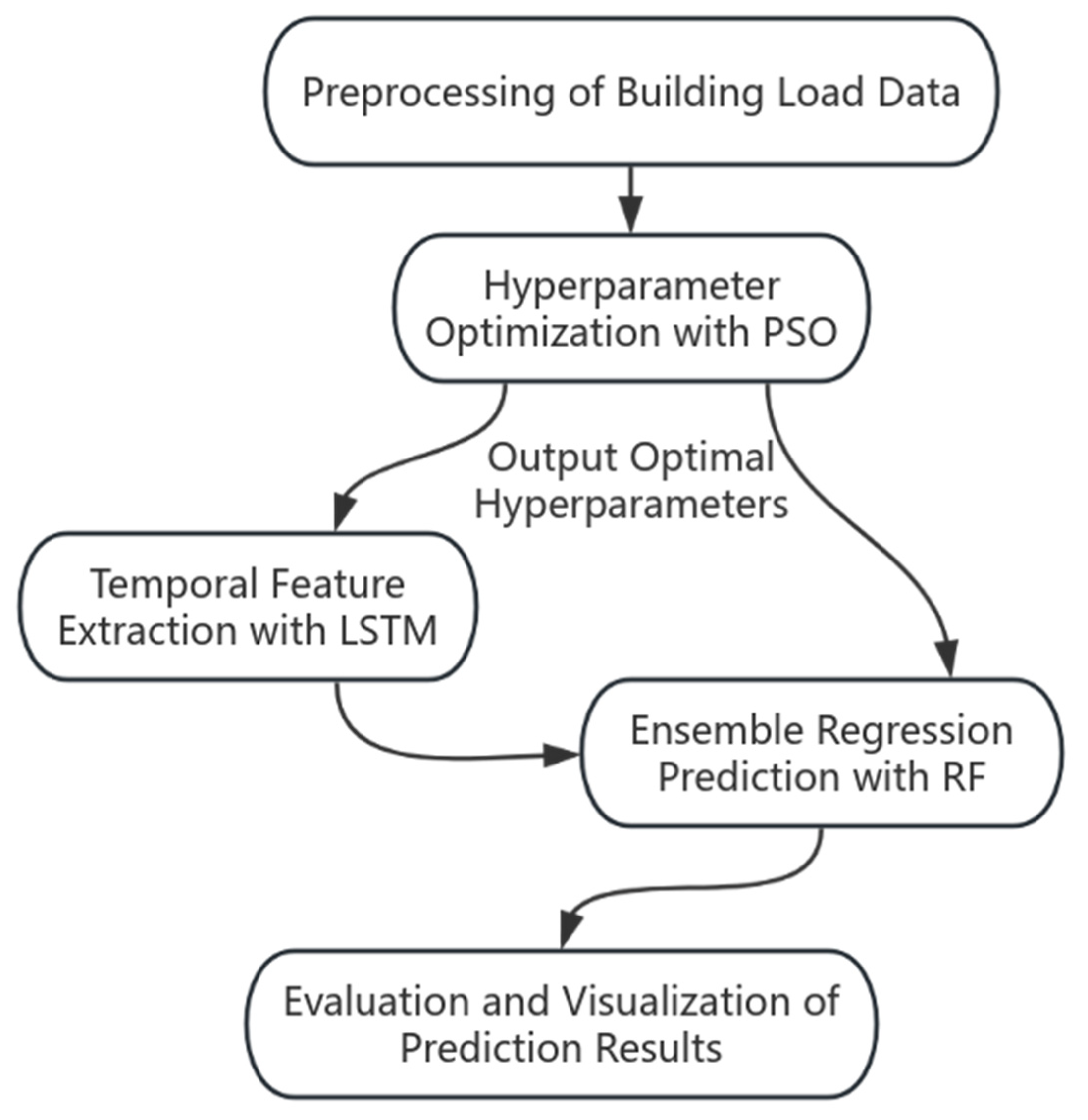
This model focuses on temporal feature extraction, multidimensional fusion, and adaptive parameter optimization. Through the collaborative operation of three key components—Particle Swarm Optimization (PSO), Long Short-Term Memory (LSTM), and Random Forest (RF)—it addresses the limited adaptability of single models in capturing the nonlinear and periodic characteristics of building loads, thereby achieving high-precision load forecasting. The functional roles and cooperative mechanisms of the three components are illustrated in Figure 2.
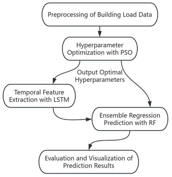
Figure 2.
PSO-LSTM-RF hybrid coordination mechanism diagram.
The three components have clearly defined responsibilities and complementary functions that jointly enhance the model’s predictive performance. As an intelligent hyperparameter optimizer, PSO employs an iterative optimization mechanism based on “individual cognition–group collaboration” to search for the optimal combination of LSTM and RF hyperparameters within a high-dimensional parameter space. This effectively alleviates overfitting risks, reduces computational redundancy, and provides a parameter foundation for subsequent model training. As a temporal feature extractor, LSTM, with its gated structure composed of forget, input, and output gates, accurately captures the long-term temporal dependencies of building loads—such as intraday fluctuation patterns and the temporal effects of meteorological factors—and transforms these dependencies into high-dimensional temporal feature vectors. As an ensemble regression predictor, RF integrates the temporal features output by LSTM with the original static features (such as building type and date attributes), and, through ensemble learning based on multiple decision trees, captures nonlinear coupling relationships among features, reduces the randomness of single-model predictions, and ultimately outputs stable and accurate building load forecasts.
To enhance the prediction accuracy and scenario adaptability of the PSO-LSTM-RF hybrid model, this study employs the PSO algorithm to optimize the core hyperparameters of the LSTM and RF modules. Based on experimental data from 18 groups (6 buildings × 3 weather conditions), the reasonable search ranges and optimal value distributions of each parameter are determined (see Appendix B Table A1 for detailed hyperparameter descriptions). The model achieves excellent predictive performance, with the R2 of the test set all greater than 0.95 and the MAPE all less than 4%. Among them, the R2 of 15 groups exceeds 0.99, and the average R2 is close to 0.985, demonstrating a highly satisfactory predictive effect.
2.3. Evaluation Model for Building Load Adjustable Margin (BAM)
This section first identifies the baseline simulation data that best align with the predicted day via a similar-day screening mechanism. Based on the selected samples, the BAM and RD are then quantified, thereby ensuring consistency throughout the entire evaluation process.
2.3.1. Similar-Day Screening Model
To ensure that the baseline scenario data align with the characteristics of the predicted day and support margin evaluation, a similar-day screening model is established. The model takes as input the load curves, meteorological parameters, and date attributes of the predicted and baseline days and conducts a two-step screening process. In the first step, similarity is quantified using five indicators: root mean square error (RMSE) and mean absolute error (MAE) reflect the amplitude difference of load curves; the Pearson correlation coefficient (r) characterizes overall trend correlation; trend similarity (ts) is calculated by comparing the sign consistency of load differences to measure local matching; and dynamic time warping (DTW) distance resolves temporal misalignment between curves. In the second step, weighted scoring and constraints are applied to refine the selection range. Specifically, the Pearson coefficient is assigned a weight of 0.9 and ts a weight of 0.1, and the normalized weighted sum of both is used as the comprehensive score. Meanwhile, temperature deviation ≤ 3 °C, humidity deviation ≤ 10.00%, and consistent date attributes are imposed as constraints. Finally, days are ranked by the comprehensive score, and the optimal similar day is selected to provide data support for EnergyPlus in generating the baseline scenario load curve.
In the second step, weighted scoring and constraints are applied to refine the selection range. Specifically, the Pearson coefficient is assigned a weight of 0.9 and ts a weight of 0.1—this weight allocation is determined by three key considerations:
- Alignment with physical relevance: Building load is strongly correlated with time and meteorological factors, so load curves of historical similar days and the target day usually show high linear correlation. The Pearson coefficient accurately quantifies core similarity at the numerical level, hence the high weight.
- Avoiding trend interference: Trend similarity (ts) only focuses on the rise/fall direction of adjacent load periods, but small fluctuations in building load have no substantial impact on overall load prediction. The low 10% weight prevents interference from such ineffective trends.
- Empirical data support: We tested multiple weight combinations (e.g., 80% + 20%, 50% + 50%, 20% + 80%, 10% + 90%) with actual data. The results show that the 90% + 10% ratio yields the highest-quality similar days, and the comparison results are shown in Appendix B Table A2.
The normalized weighted sum of both is used as the comprehensive score. Meanwhile, temperature deviation ≤ 3 °C, humidity deviation ≤ 10.00%, and consistent date attributes are imposed as constraints. Finally, days are ranked by the comprehensive score, and the optimal similar day is selected to provide data support for EnergyPlus in generating the baseline scenario load curve.
To further validate the validity of the above similar-day screening approach, we cross-checked the load response generated by EnergyPlus (based on the selected optimal similar-day baseline) against the historical real load data. While a numerical deviation of approximately 10% is observed between the simulated load and the real load, their core fluctuation patterns—including peak–valley occurrence timings and temporal variation trends—remain highly consistent. The visualization of this comparison is provided in Appendix A Figure A1 to support the reliability of the similar-day-derived baseline data.
2.3.2. Building Adjustable Margin (BAM) Calculation Model
The physical meaning of the adjustable load margin is the absolute value of the load difference between the baseline and response scenarios at the same 5 min time step, representing the load adjustment potential. The calculation formula is given in Equation (1):
where is the adjustable load margin (kW) of the -th response scenario at the -th 5 min time step, , corresponding to S1–S4; is the time step index (12 steps per hour); is the load value (kW) of the baseline scenario at the -th time step; is the load value (kW) of the -th response scenario at the same time step.
2.3.3. Response Duration (RD) Calculation Model
The RD is defined as the time interval between the air-conditioning shutdown moment and the point when the indoor temperature rises to 28 °C and the system restarts, representing the duration of the adjustment capability. The calculation formula is shown in Equation (2):
where is the RD (h, rounded to two decimal places) of the -th response scenario; is the preset air-conditioning shutdown time in the -th scenario (24 h format, e.g., S1 = 10:00); is the actual restart time in the -th scenario, determined by EnergyPlus based on 5 min indoor temperature data as the first time step where temperature ≥ 28 °C.
3. Model Construction and Scenario Settings
This chapter focuses on the data foundation for load forecasting and the scenario framework for margin evaluation. Through data preprocessing, typical building modeling, and energy simulation setup, standardized datasets and simulation environments are established to support subsequent analysis.
3.1. Data Preprocessing
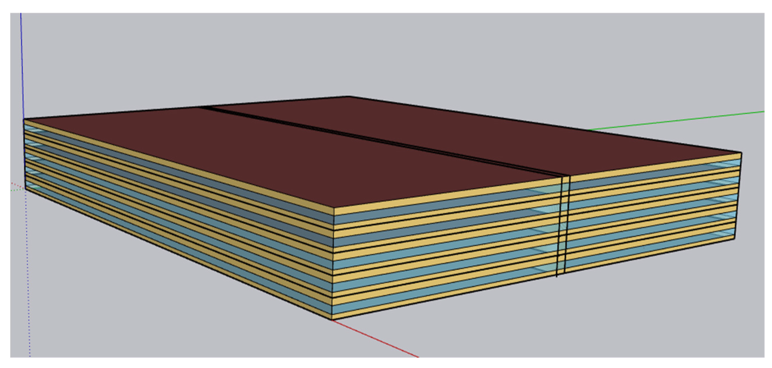
Based on hourly operational data (Building Management System) and meteorological data (weather stations) from three types of actual buildings—office, shopping mall, and hotel—in Shanghai from 1 May to 30 September 2023, high-quality data samples were obtained through a four-step preprocessing procedure (Table 2). The physical models of the three typical buildings, established using SketchUp(2024) and OpenStudio(1.8.0), are visualized in Figure 3, which illustrates the core structural characteristics consistent with the actual buildings selected for data collection.

Table 2.
Data preprocessing procedures.
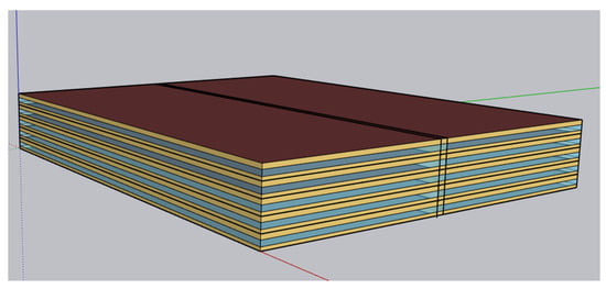
Figure 3.
3D diagram of the building model.
3.2. Modeling of Three Typical Building Types
3.2.1. Establishment of Typical Physical Models
To reduce simulation complexity and ensure generality of results, three typical building physical models were developed using SketchUp and OpenStudio. The basic parameters of each model are listed in Table 3.

Table 3.
Key parameters of typical building models.
3.2.2. Establishment of Typical Energy Models
- Building envelope settings:
According to the design characteristics of public buildings in hot summer and cold winter regions, the material and envelope parameters were configured based on the General Code for Energy Conservation and Renewable Energy Utilization in Buildings (GB55015-2021) [34], as detailed in Appendix B Table A3 and Table A4.
- 2.
- Internal disturbance parameters:
In accordance with GB55015-2021, internal gains from occupants, lighting, and appliances were defined as listed in Table 4.

Table 4.
Internal disturbance parameters of buildings.
3.3. Energy Simulation Settings
Following the logic of using the baseline scenario as a reference and the response scenarios to evaluate flexibility potential, a dual-scenario simulation framework was established with the following configurations:
- Baseline scenario:
Air-conditioning operates from 08:00 to 18:00 (target indoor temperature: 24 °C), and remains off during other hours. The simulation uses the Shanghai Typical Meteorological Year (TMY) weather file and outputs 5 min load profiles, which serve as the benchmark for model prediction comparison.
- 2.
- Response scenarios:
All parameters of the baseline scenario are retained, with only the air-conditioning on/off schedule modified (Table 5) to simulate demand-response processes. To clarify how the Energy Management System (EMS) implements the adjusted air-conditioning schedule in response scenarios, the setting logic of the EMS system is visualized in Figure 4. It illustrates the linkage between schedule modification (Table 5) and real-time load control in the EMS, which ensures the consistency of scenario execution. The resulting 5 min load profiles are used for adjustable margin calculation.

Table 5.
Air-conditioning control logic.

Figure 4.
EMS setting logic for demand-response schedule in response scenarios.
4. Data and Results Analysis
4.1. Load Prediction Results Analysis
Following the logic of accuracy indicators, model comparison, and scenario adaptation, this section emphasizes key data and core conclusions, omitting repetitive single-building details to highlight general patterns.
4.1.1. Core Prediction Accuracy
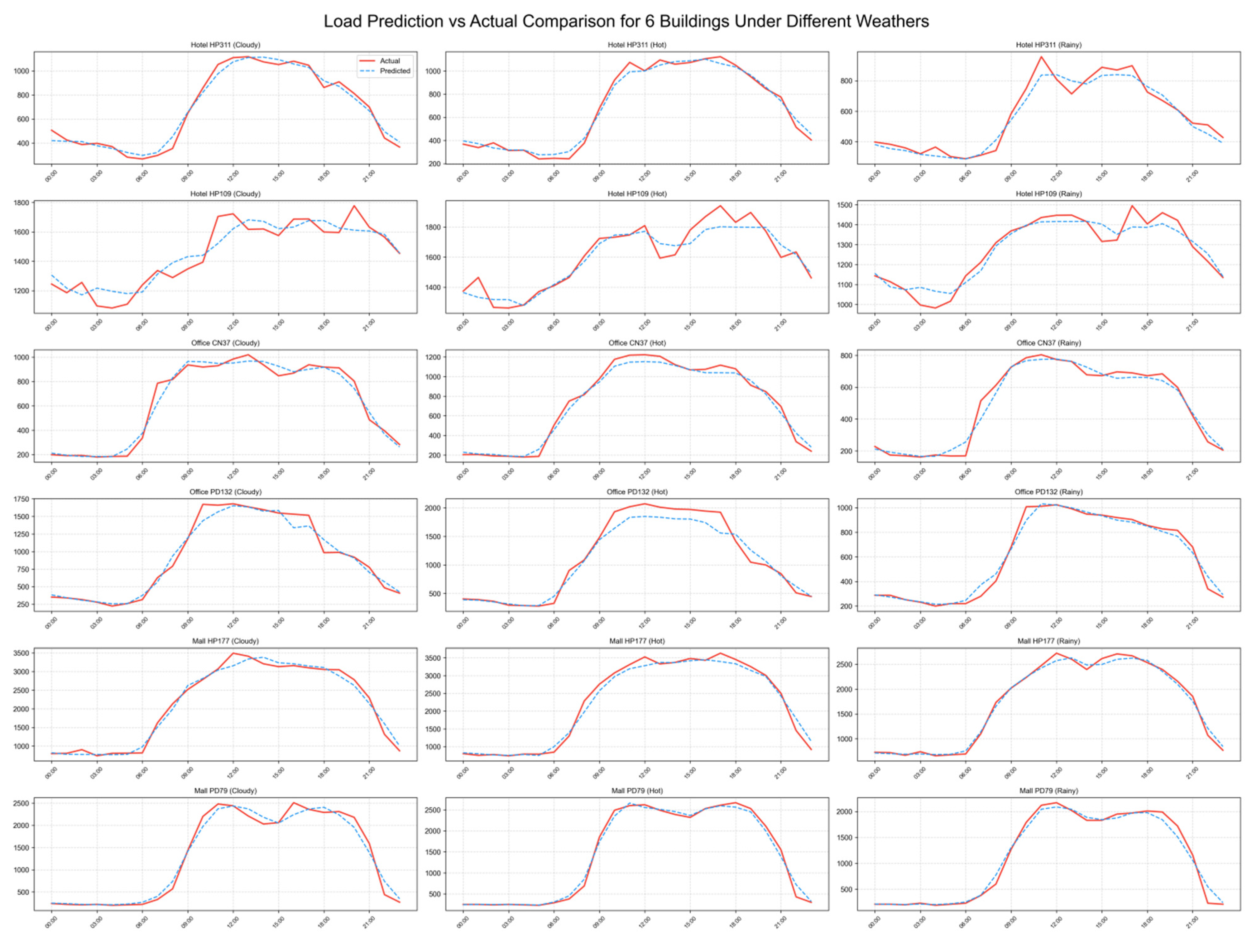
The PSO-LSTM-RF model performs excellently across three building types and three weather scenarios, achieving an average R2 of 0.985 on the test set, with MAPE controlled between 1.92% and 5.75%. The RMSE varies proportionally with the magnitude of building load. Figure 5 presents the comparison of load predictions for six buildings under different weather conditions.
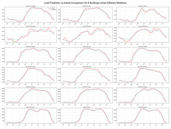
Figure 5.
Comparison of prediction results.
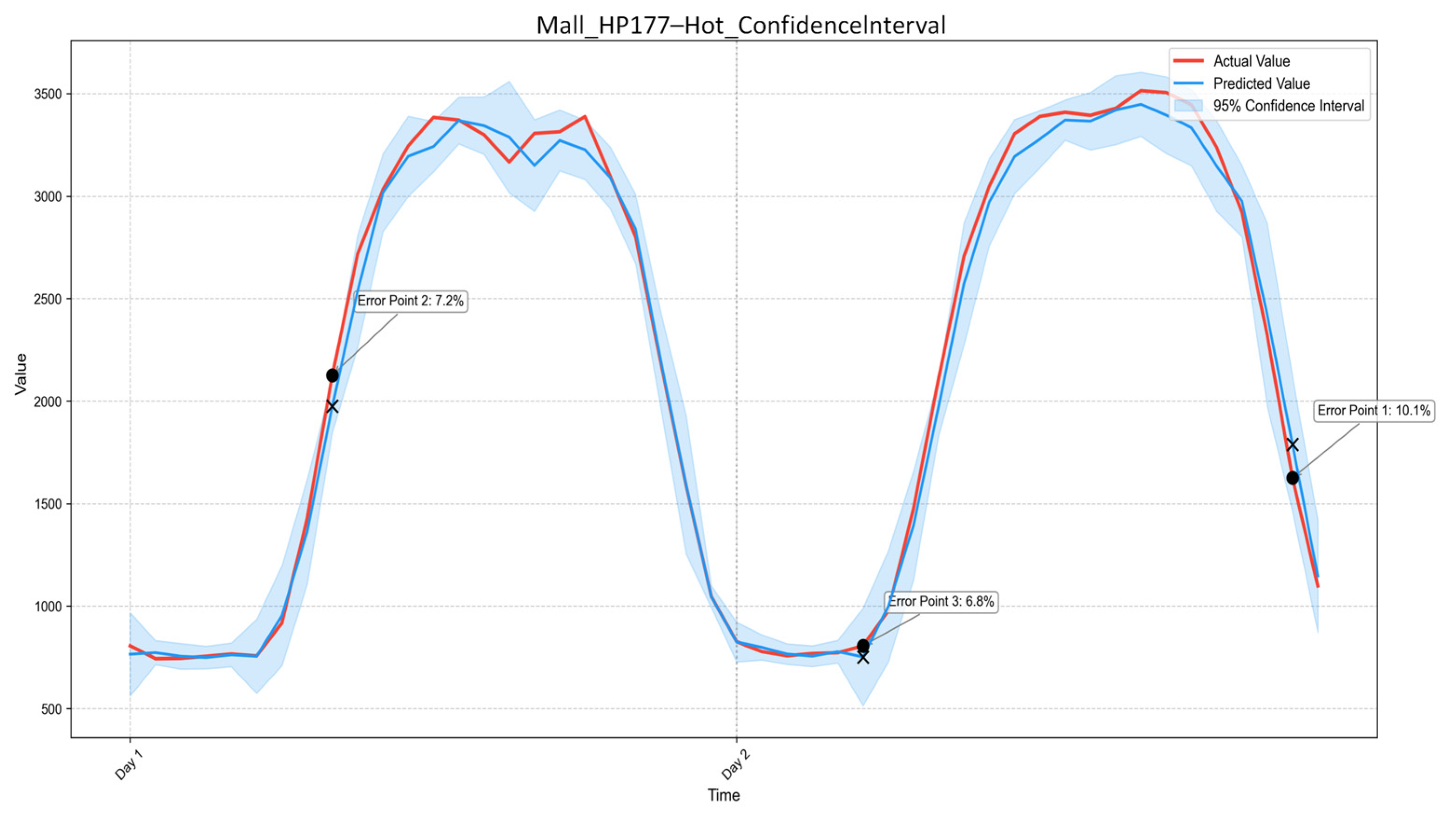
To further verify the model’s statistical reliability, 95% confidence intervals for load prediction results of three building types across various weather scenarios were calculated. Taking mall buildings under hot conditions as a representative case (Figure 6), predicted values lie entirely within the 95% confidence interval, with a maximum error of only 10.1%—illustrating the model’s high statistical reliability for commercial buildings with stable load patterns. Hotel buildings show a maximum error of 14.9% under hot conditions, while office buildings exhibit larger fluctuations (peak error 43.1% under hot conditions), driven by complex load changes from frequent air-conditioning adjustments and personnel flow. Detailed confidence interval results for other cases are provided in Appendix A Figure A2, Figure A3, Figure A4, Figure A5, Figure A6, Figure A7, Figure A8 and Figure A9.
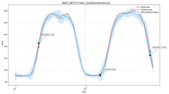
Figure 6.
Load curve with 95% confidence interval for Mall_HP177-Hot.
4.1.2. Model Prediction Comparison
- PSO Optimization convergence curve
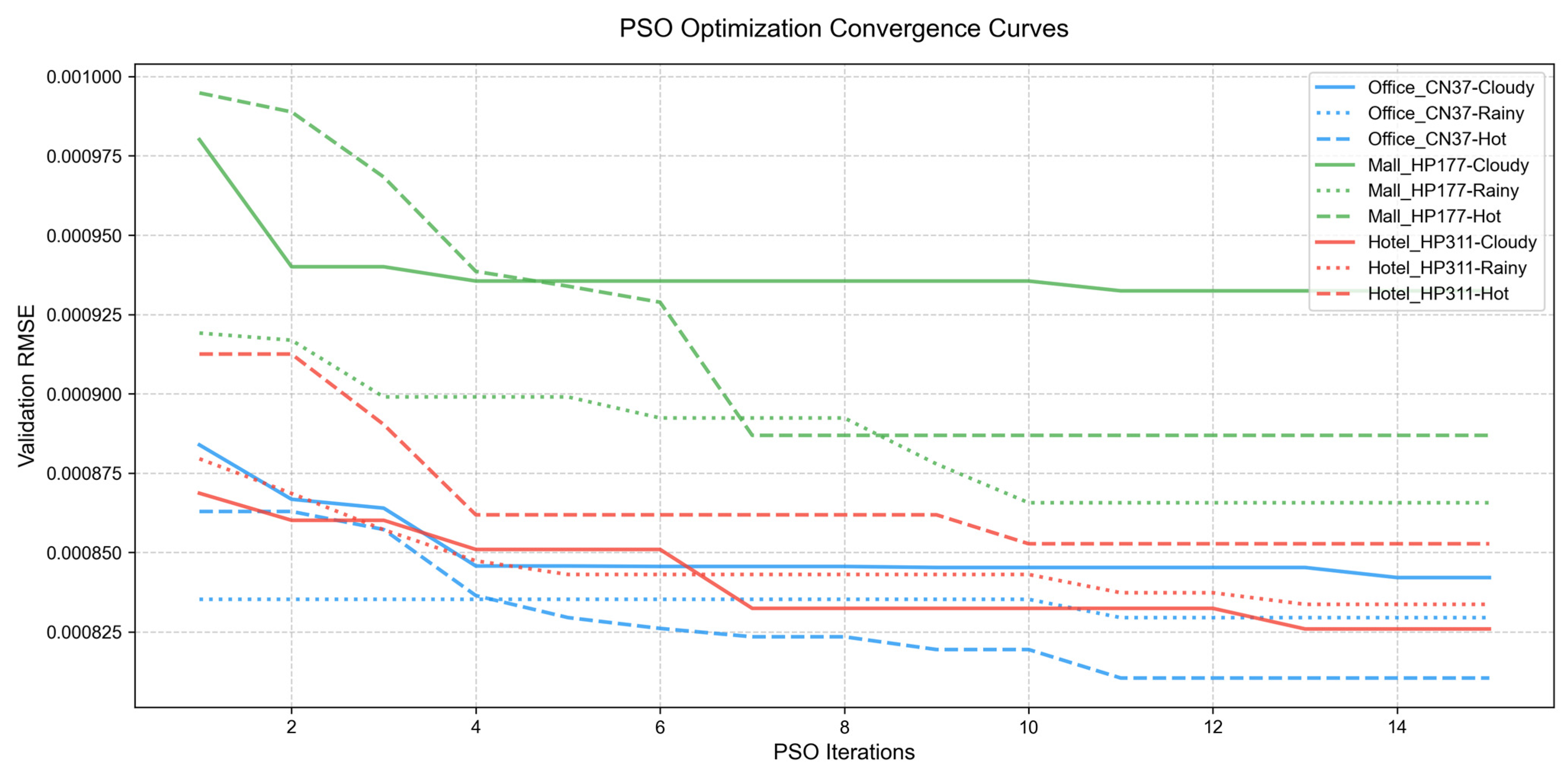
The core of PSO lies in iteratively searching and optimizing the model’s hyperparameters, ultimately allowing the validation error to converge to a stable range. All convergence curves exhibit a “rapid decline followed by stabilization” pattern, confirming the effectiveness of PSO in hyperparameter optimization, as shown in Figure 7. The influence of building type on optimization difficulty follows the order of hotel > shopping mall > office building. High-temperature days pose the greatest challenge for optimizing office building models, while rainy conditions tend to cause late-stage error fluctuations in hotel models.
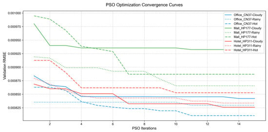
Figure 7.
PSO optimization convergence curves across buildings and scenarios.
- 2.
- Multimodel error boxplot
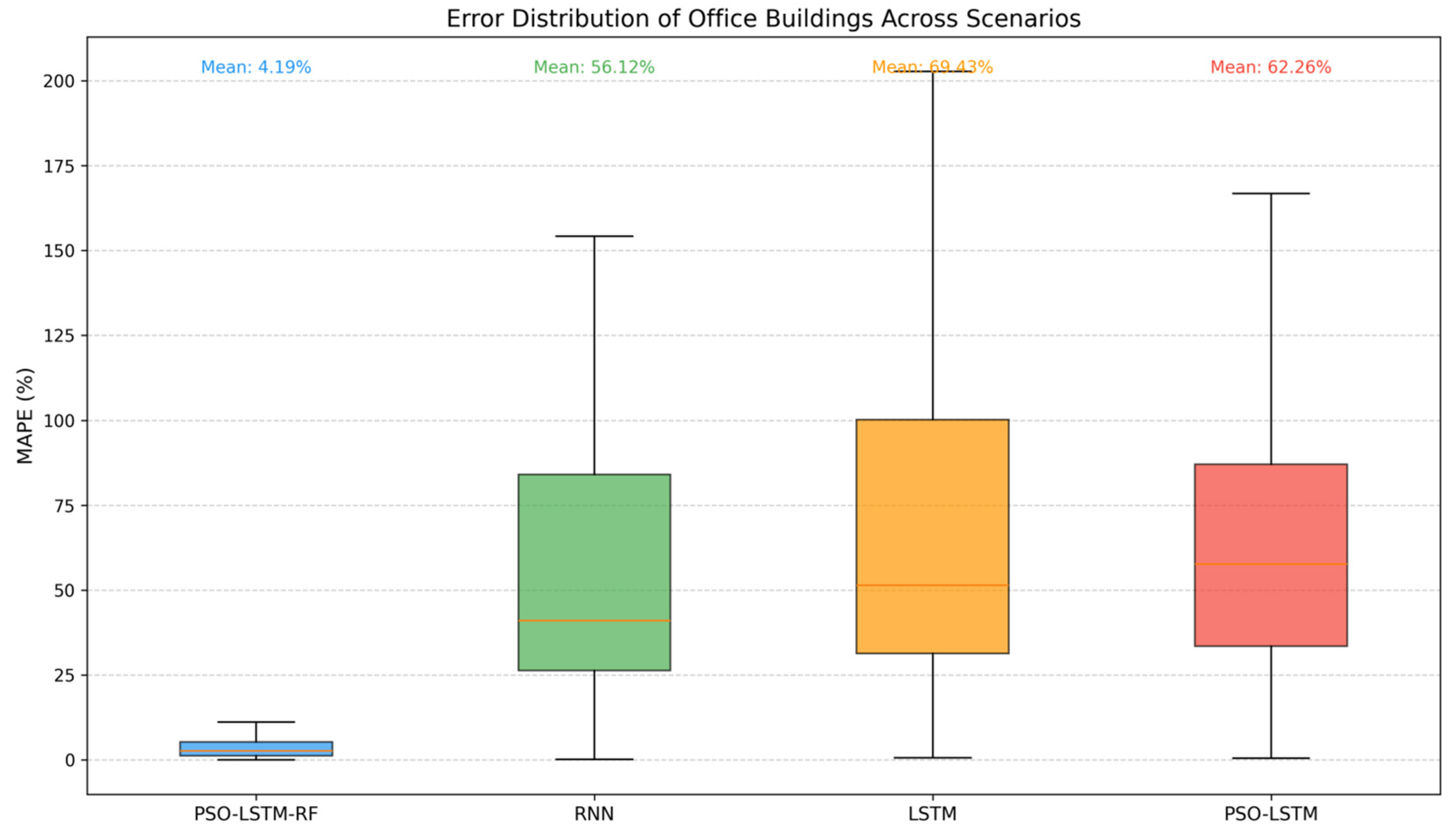
This section primarily presents the error analysis charts for office buildings, while the corresponding charts for shopping malls and hotels are moved to the appendix due to space limitations. Details can be found in Appendix A (Figure A10 and Figure A11) and Appendix B (Table A5 and Table A6). Figure 8 and Table 6 presents the error analysis results for office buildings. From the model perspective, the PSO-LSTM-RF exhibits significantly lower mean errors and smaller fluctuations compared to RNN, LSTM, and PSO-LSTM, confirming the effectiveness of the PSO optimization and LSTM-RF hybrid architecture in building load prediction. From the perspective of building type, the ranking of model performance is consistent across all three types: PSO-LSTM-RF performs best, followed by PSO-LSTM, RNN, and LSTM, indicating that the proposed architecture demonstrates universality and robustness, independent of building function differences.
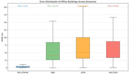
Figure 8.
Error boxplots of office buildings under multiple scenarios.

Table 6.
Comparison of prediction errors for office buildings across models.
4.1.3. Scenario Prediction Comparison
- Overall adaptability of load prediction under different weather scenarios
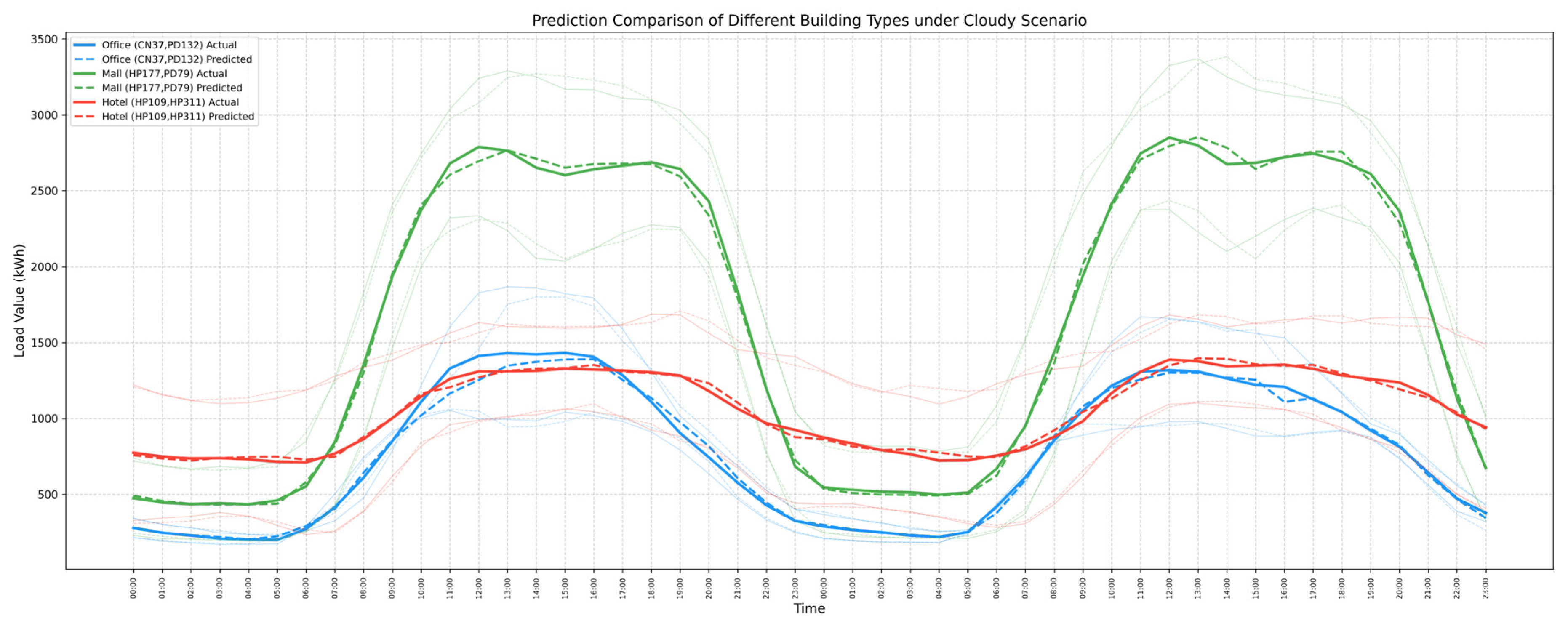
Building load characteristics vary significantly under different weather conditions, and the PSO-LSTM-RF model exhibits strong scenario adaptability by capturing both macro-trends and micro-fluctuations. As shown in Figure 9, the predicted load curves of the three building types are highly consistent with the actual curves under high-temperature, cloudy, and rainy days. Specific performance and load characteristics are analyzed in Figure 9, Appendix A Figure A12 and Figure A13, and Table 7.
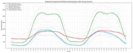
Figure 9.
Building load prediction under windy conditions.

Table 7.
Analysis of building load prediction under different weather conditions.
- 2.
- Sensitivity of prediction error to weather types
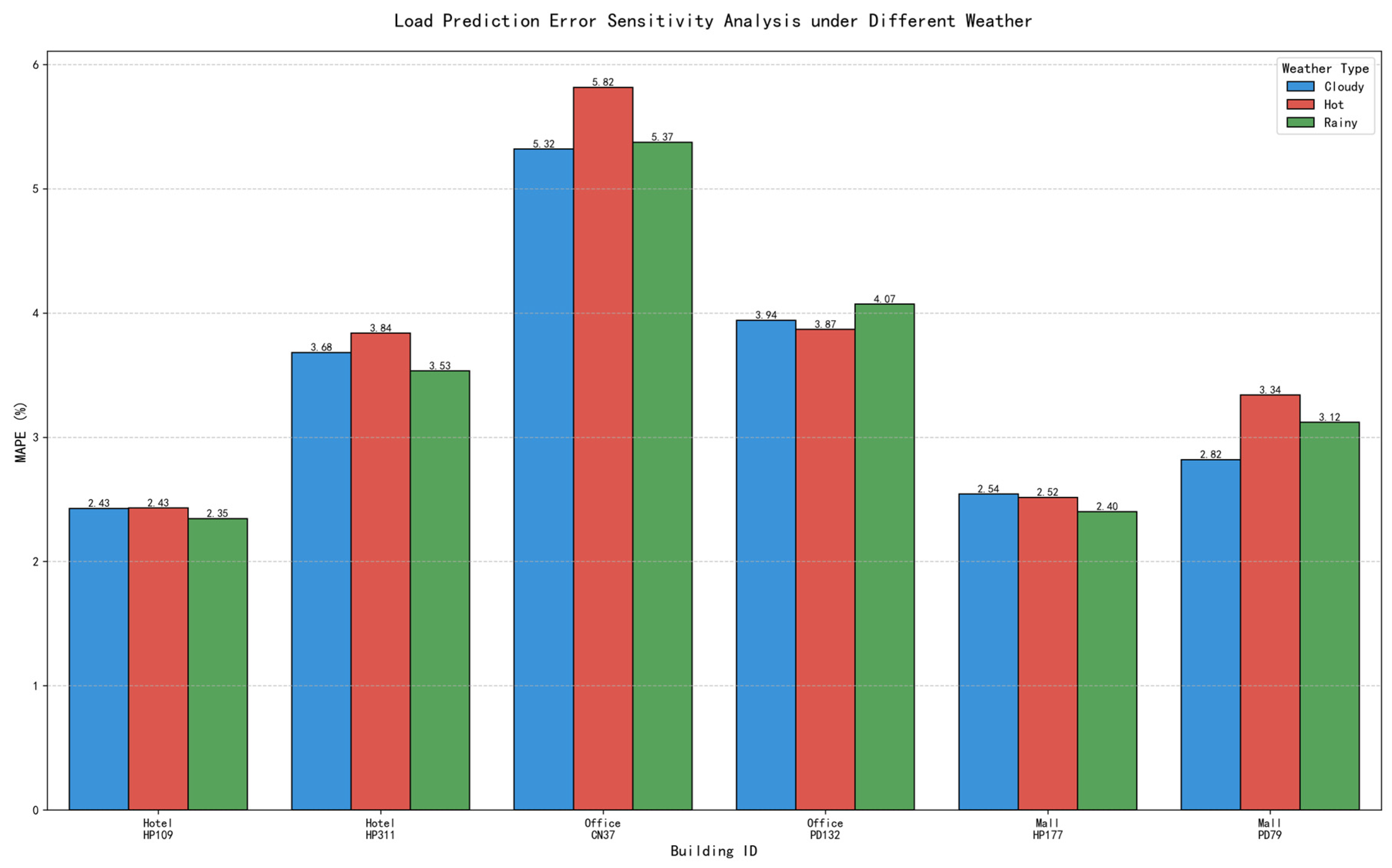
To further clarify the impact of weather factors on prediction accuracy, we conducted a sensitivity analysis of load prediction errors under different weather scenarios (Figure 10). The results show that the prediction error of office buildings (e.g., CN37) is relatively higher (5.82%) under hot weather (attributed to complex load fluctuations from intensive air-conditioning adjustment in high temperatures), while the error of hotel and mall buildings remains stable across weather types (maximum error ≤ 3.84%). This analysis verifies the model’s robustness in most scenarios and identifies key weather conditions for subsequent parameter optimization.
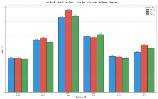
Figure 10.
Load prediction error sensitivity analysis under different weather.
- 3.
- Refined characteristics of prediction errors by time period and scenario
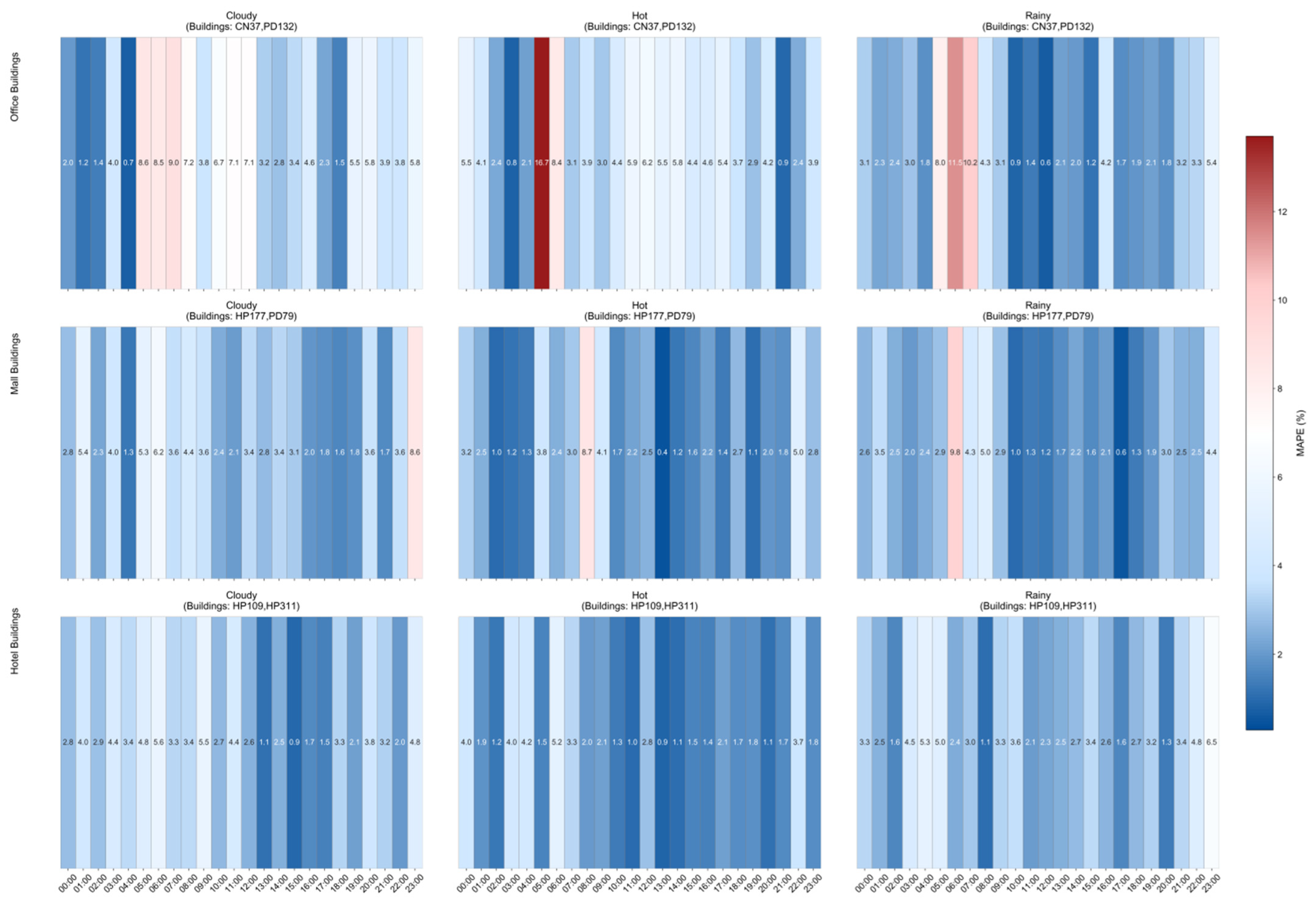
The above analysis clarifies the macro-level impacts of different weather scenarios on building loads and model prediction performance. Further examining the temporal dimension, time-period-based heatmaps reveal the distribution patterns of model prediction errors across scenarios, as shown in Figure 11.
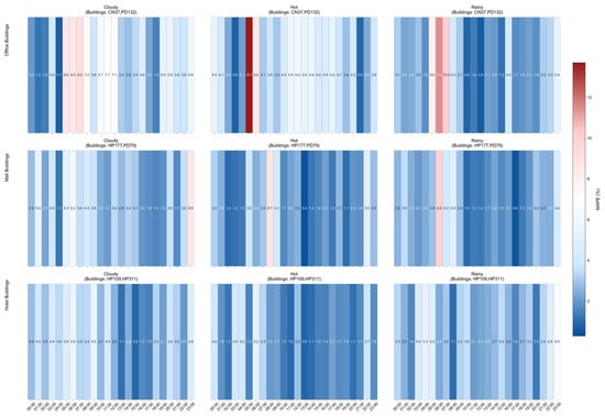
Figure 11.
Time-segmented error heatmap.
For office buildings, during peak load periods (9:00–18:00), the influence of air-conditioning regulation under high-temperature conditions causes prediction errors to be 1.20–1.80% higher than those during off-peak hours (0:00–6:00), where errors remain below 1.50%.
For shopping malls, time-period differences are the most pronounced: during peak hours (10:00–22:00), strong load fluctuations induced by customer flow and weather coupling result in errors of 8.00–12.00%; during off-peak hours (0:00–8:00), rainy weather causes grid voltage disturbances, increasing errors by about 1.50% compared with other weather conditions.
For hotels, time-period differences are the smallest. Both peak (18:00–2:00) and off-peak (8:00–14:00) errors remain at ≤3.20%, as the rigidity of occupancy rates mitigates weather impacts, leading to gradual load changes and the lowest model fitting difficulty.
4.2. Analysis of Actual Flexibility Simulation Results
4.2.1. Quantitative Evaluation of EAM
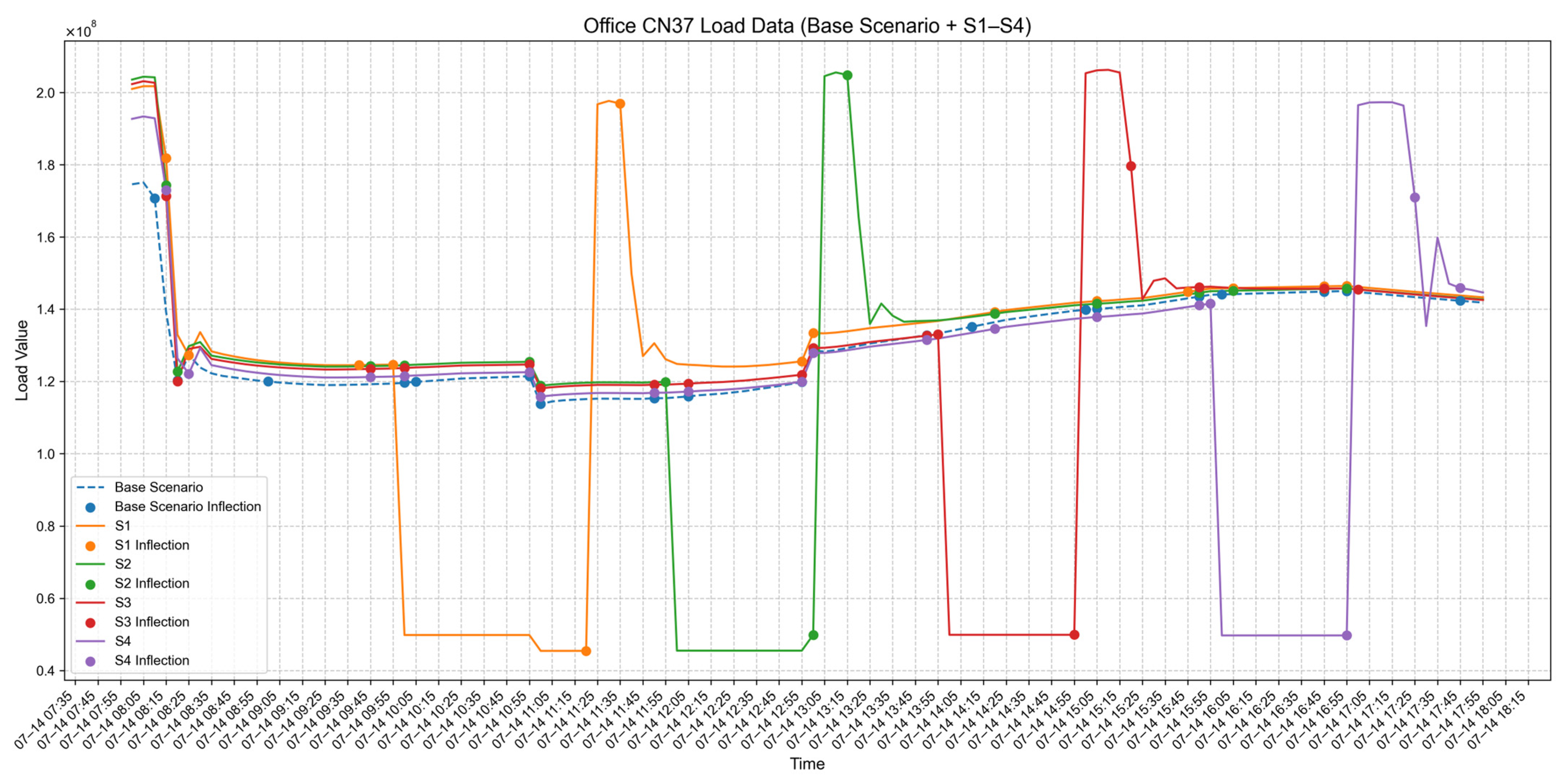
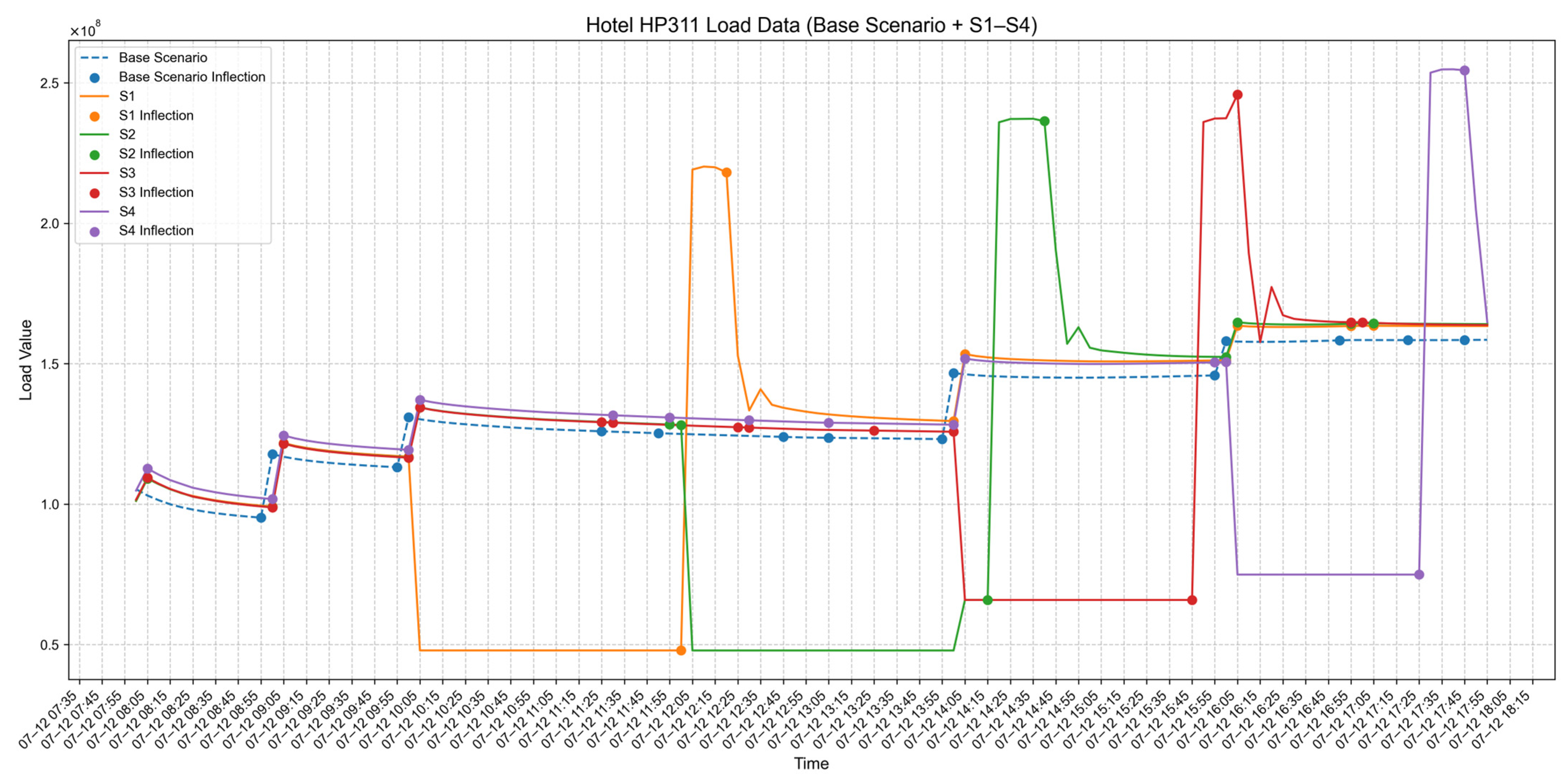
Based on the matched samples output by the similar-day screening model, the BAM and RD were quantified for four response scenarios (S1–S4) of three building types: office, shopping mall, and hotel. This section presents only the results for office buildings (Figure 12, Table 8). Corresponding analyses for shopping malls and hotels are provided in Appendix A (Figure A14 and Figure A15) and Appendix B (Table A7 and Table A8).
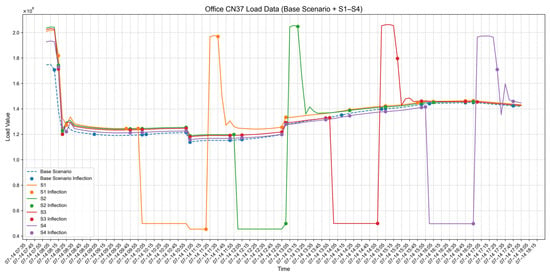
Figure 12.
Load profiles of office buildings under different response scenarios.

Table 8.
Evaluation of BAM for office buildings across scenarios.
- Office buildings
The BAM of office buildings exhibits a pronounced dependence on time of day. In the S1 scenario, the BAM reaches 332.48 kWh, with an RD of 75 min, representing the optimal values among all scenarios. This is due to sufficient indoor thermal storage in the early morning and moderate outdoor temperatures; after turning off the air-conditioning, the indoor temperature rises to 28 °C relatively slowly, creating a larger adjustment space.
In the S2 scenario, the BAM decreases to 261.71 kWh, with a shortened RD of 65 min, mainly because the outdoor temperature rises around noon, increasing the building’s heat exchange with the environment and accelerating the indoor thermal accumulation rate.
For the S3 and S4 scenarios, the BAM are 290.53 kWh and 316.28 kWh, respectively, with both RD stabilizing at 60 min. This reflects that from the afternoon to evening, the building’s thermal storage capacity approaches saturation, and the precision of indoor temperature control increasingly constrains the flexibility margin.
- 2.
- Shopping mall buildings
Due to their large floor area, high thermal storage capacity of the envelope, and stable internal occupancy, lighting, and equipment loads, shopping mall buildings exhibit a “high absolute value, low fluctuation” characteristic in adjustable margin. In the S1 scenario, the adjustable margin reaches 446.12 kWh, while in the S4 scenario it is 417.45 kWh. The S2 and S3 scenarios are 394.60 kWh and 361.22 kWh, respectively, with a maximum difference of only 84.9 kWh across scenarios, far lower than that of office and hotel buildings. Regarding RD, the S1–S3 scenarios are all 60 min, while the S4 scenario is extended to 75 min, mainly because outdoor temperatures decrease after 16:00 and the proportion of fresh air operation during evening hours increases, slowing the indoor temperature rise. This characteristic endows shopping mall buildings with the capacity to meet large-scale, long-duration load reduction demands, demonstrating potential as a core regulation resource.
- 3.
- Hotel buildings
Hotel buildings exhibit an “afternoon peak, decreasing over time” pattern in adjustable margin. In the S2 scenario, the BAM reaches 579.27 kWh, with RD of 135 min, representing the maximum among all scenarios across the three building types. This is attributed to stable room occupancy at noon, consistent indoor heat generation from occupants and equipment, and the effective thermal insulation of the envelope, which maintains indoor thermal balance after the air-conditioning is turned off. In the S1 scenario, the BAM is 526.88 kWh with RD of 120 min, still at a relatively high level. For the S3 (air-conditioning off at 14:00) and S4 (off at 16:00) scenarios, the BAM decreases to 463.44 kWh and 393.01 kWh, with RD shortened to 105 min and 85 min, reflecting the impact of afternoon and evening room usage changes on the building’s thermal balance, which reduces the available regulation space.
4.2.2. Discussion on Factors Influencing Building Adjustable Margin (BAM)
1. Building type dominates flexibility characteristics: shopping mall buildings, relying on strong thermal storage capacity and stable internal disturbances during operating hours, exhibiting high absolute BAM with minimal variation across scenarios, making them suitable for large-scale, long-duration load reduction. Hotel buildings, with highly insulated guest room areas and stable thermal conditions at noon, achieve significant peak BAM and are preferred carriers for deep load shaving in the grid. Office buildings have BAM between the two, but their nine-to-five schedules produce pronounced load patterns, and implementing response strategies causes minimal disruption to daily office operations, enhancing practical applicability.
2. Scenario selection must precisely match building characteristics: for office buildings, the S1 scenario, with air-conditioning turned off at 10:00, should be prioritized. This scenario achieves a BAM of 332.48 kWh and an RD of 75 min; the early-morning thermal storage is sufficient, and there is no interference from peak occupancy periods, making it the optimal choice for balancing regulation effectiveness and operational convenience. For shopping mall buildings, differences in BAM among scenarios are small; the S4 scenario, due to high fresh air operation in the evening, extends the RD to 75 min, making it suitable for evening peak shaving and full-time response potential utilization. For hotel buildings, the S2 scenario should be prioritized, with a BAM of 579.27 kWh and an RD of 135 min; the stable thermal environment and constant internal loads at noon maximize the high reduction potential.
5. Conclusions and Future Work
5.1. Conclusions
This study investigated the prediction and evaluation of practical flexibility margins for typical public buildings under different operating scenarios. By integrating a PSO-LSTM-RF load forecasting model with EnergyPlus-based building energy simulation, a unified framework for load prediction, scenario simulation, and flexibility margin assessment was established. Case studies were conducted for office buildings, shopping malls, and hotels under representative summer conditions, including high-temperature, cloudy, and rainy days. The main conclusions are summarized as follows:
1. The proposed PSO-LSTM-RF model provides stable and accurate load prediction across different buildings and weather conditions. By combining particle swarm optimization, deep learning, and ensemble learning, the proposed model effectively overcomes the limited generalization and parameter sensitivity of single prediction models. It maintains high forecasting stability during peak load periods and demonstrates strong adaptability across different building types and operating scenarios.
2. The EnergyPlus-based dual-scenario simulation framework enables refined quantification of building flexibility characteristics. The baseline scenario supports reliable similar-day selection, while multiple response scenarios capture load response potential under different control strategies. The simulation results reveal distinct flexibility patterns among building types: shopping malls exhibit high and stable adjustable margins due to strong thermal storage and steady internal loads; hotels achieve significant peak flexibility and high energy reduction efficiency owing to favorable thermal insulation and stable midday thermal conditions; office buildings present moderate flexibility margins while allowing response strategies with minimal disruption to normal operation.
3. The entire technical framework achieves practical implementation through a data-driven closed loop; load forecasts generated by the PSO-LSTM-RF model provide the basis for flexibility evaluation, while EnergyPlus simulations supply hourly energy consumption data for baseline and response scenarios. Through similar-day selection and margin calculation, BAM and RD are jointly quantified as the energy difference between baseline and response scenarios and the duration between air-conditioning shutdown and restart. Across all scenarios, RD ranges from 60 to 135 min, and BAM varies between 261.71 and 579.27 kWh, while indoor thermal comfort is maintained with temperatures not exceeding 28 °C. These results define practically achievable flexibility boundaries and provide quantitative guidance for selecting suitable demand-response strategies for different building types, supporting virtual power plant aggregation, grid-interactive operation, and coordinated energy system optimization.
5.2. Future Work
To further expand the research depth and practical value of this work, future research can focus on the following directions:
- Extend to special-function and underground buildings (e.g., hospitals, data centers, underground offices), optimizing the PSO-LSTM-RF model’s feature dimensions to adapt to their rigid load characteristics and unique energy consumption logic.
- Introduce dynamic indoor temperature thresholds aligned with human comfort models, enhancing the human-centric applicability of load margin evaluation.
- Combine electricity market mechanisms to explore market-oriented trading of building flexibility resources, promoting the transition from technical assessment to practical application.
Author Contributions
Conceptualization, B.X.; methodology, B.X.; data curation, W.Z., Y.Y. (Yiming Yuan), X.C., X.L., C.F., J.W., F.Q., Y.Y. (Yongwen Yang) and S.L.; writing—original draft, B.X.; writing—review and editing, L.Z.; visualization, W.Z., Y.Y. (Yiming Yuan), X.C., X.L., C.F., J.W., F.Q., Y.Y. (Yongwen Yang) and S.L.; supervision, L.Z.; project administration, L.Z. All authors have read and agreed to the published version of the manuscript.
Funding
This research was funded by the technology project of State Grid Shanghai Municipal Electric Power Company in China, grant number SGSHPD00ZSJS2413049.
Data Availability Statement
The original contributions presented in this study are included in the article. Further inquiries can be directed to the corresponding author.
Conflicts of Interest
Authors Bangpeng Xie, Chaoran Fu, Wenkai Zhao, Jiayu Wang, Yiming Yuan and Xiaoyi Chen were employed by the State Grid Shanghai Pudong Electric Power Supply Company. The remaining authors declare that the research was conducted in the absence of any commercial or financial relationships that could be construed as a potential conflict of interest.
Appendix A
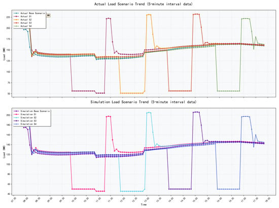
Figure A1.
Actual vs. simulation load scenario trend comparison.
Figure A1.
Actual vs. simulation load scenario trend comparison.
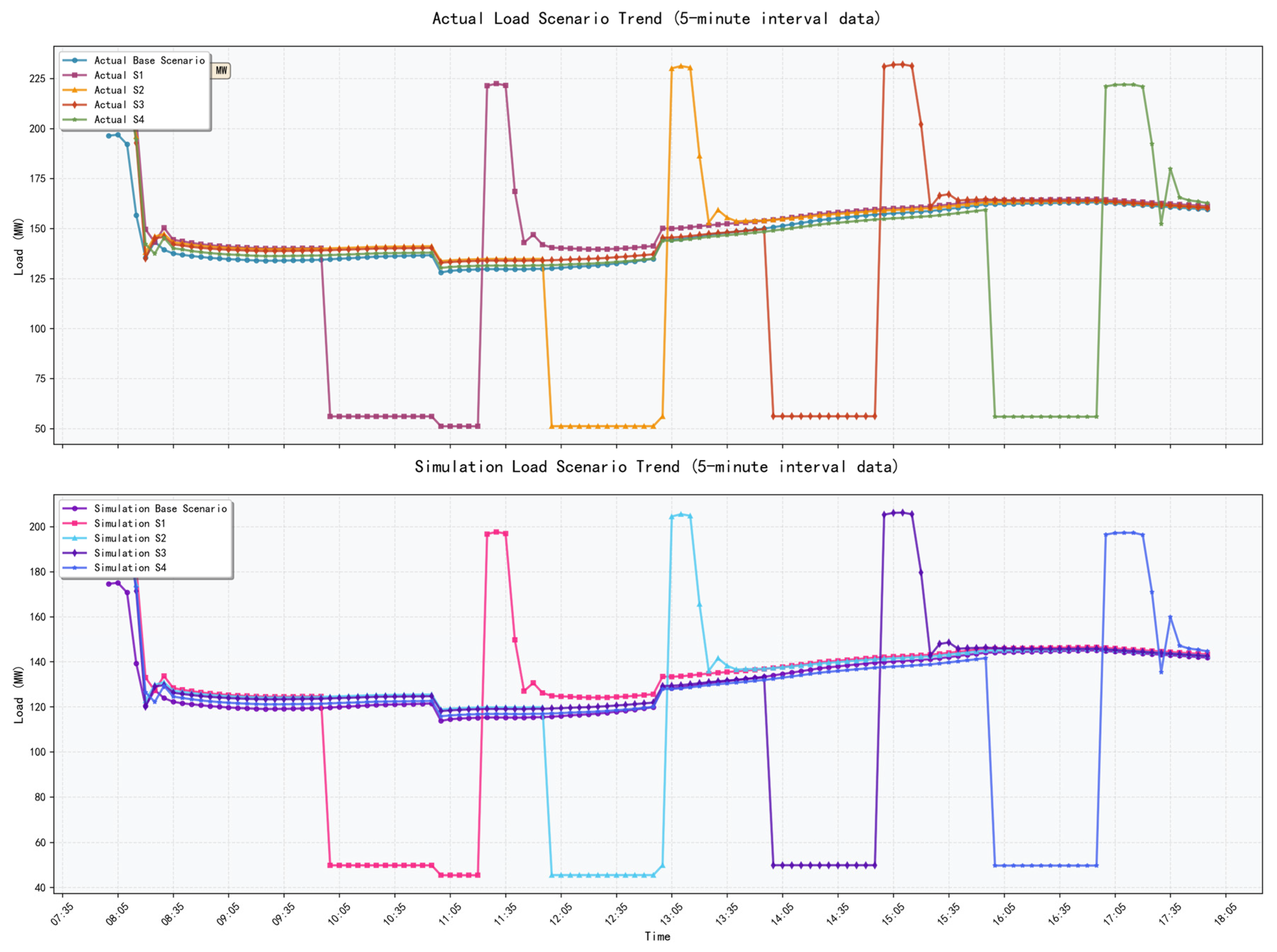
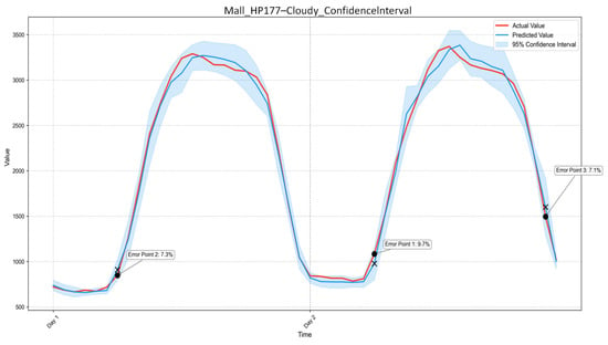
Figure A2.
Load curve with 95% confidence interval for Mall_HP177-Cloudy.
Figure A2.
Load curve with 95% confidence interval for Mall_HP177-Cloudy.
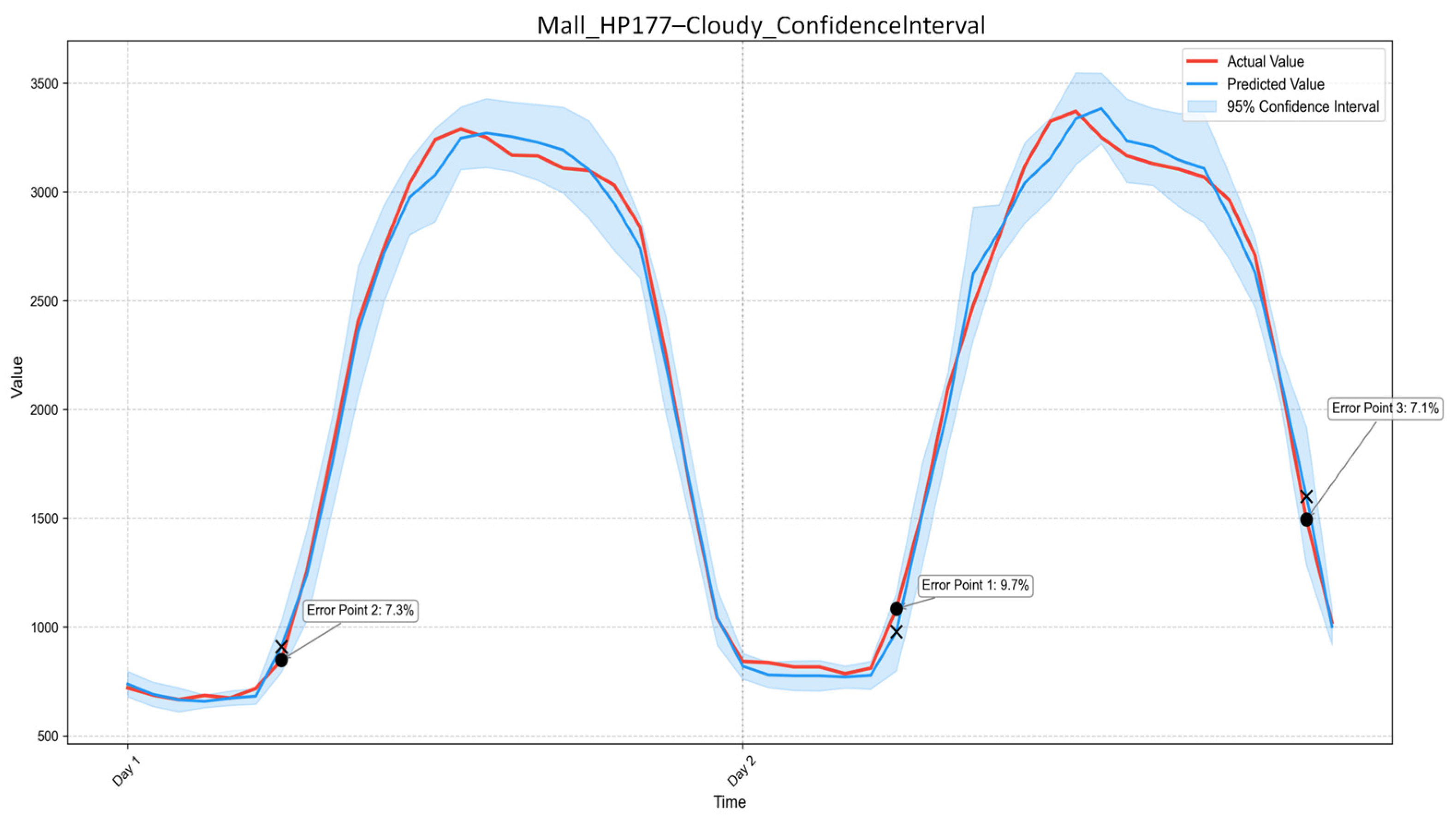
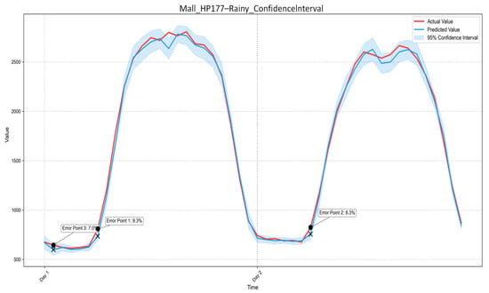
Figure A3.
Load curve with 95% confidence interval for Mall_HP177-Rainy.
Figure A3.
Load curve with 95% confidence interval for Mall_HP177-Rainy.
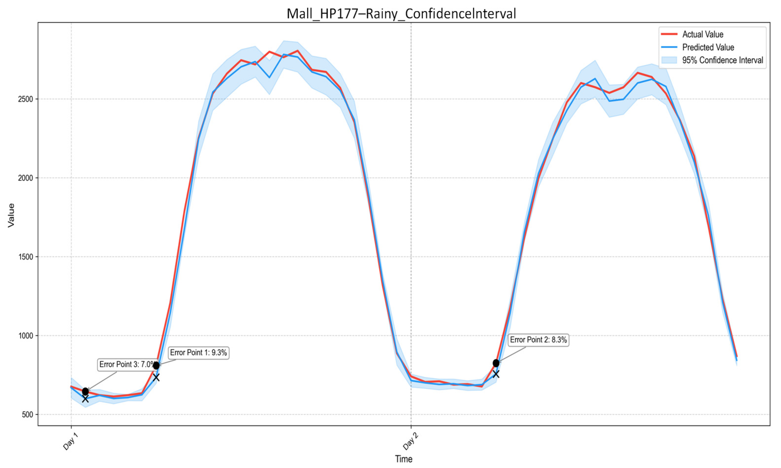
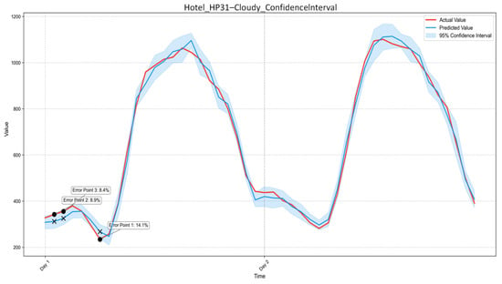
Figure A4.
Load curve with 95% confidence interval for Hotel_HP311-Cloudy.
Figure A4.
Load curve with 95% confidence interval for Hotel_HP311-Cloudy.
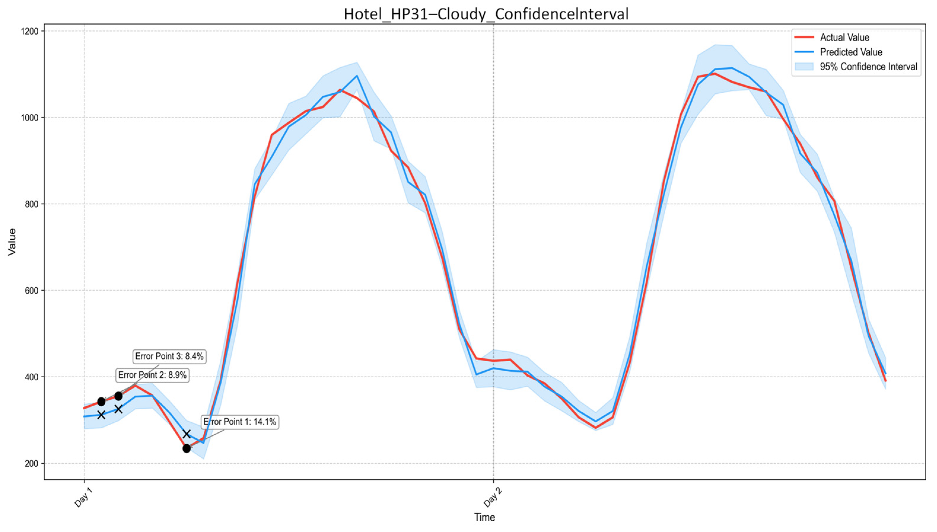
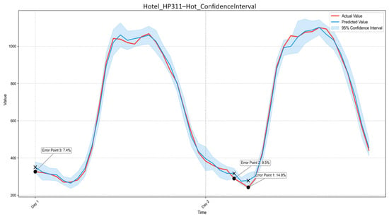
Figure A5.
Load curve with 95% confidence interval for Hotel_HP311-Hot.
Figure A5.
Load curve with 95% confidence interval for Hotel_HP311-Hot.
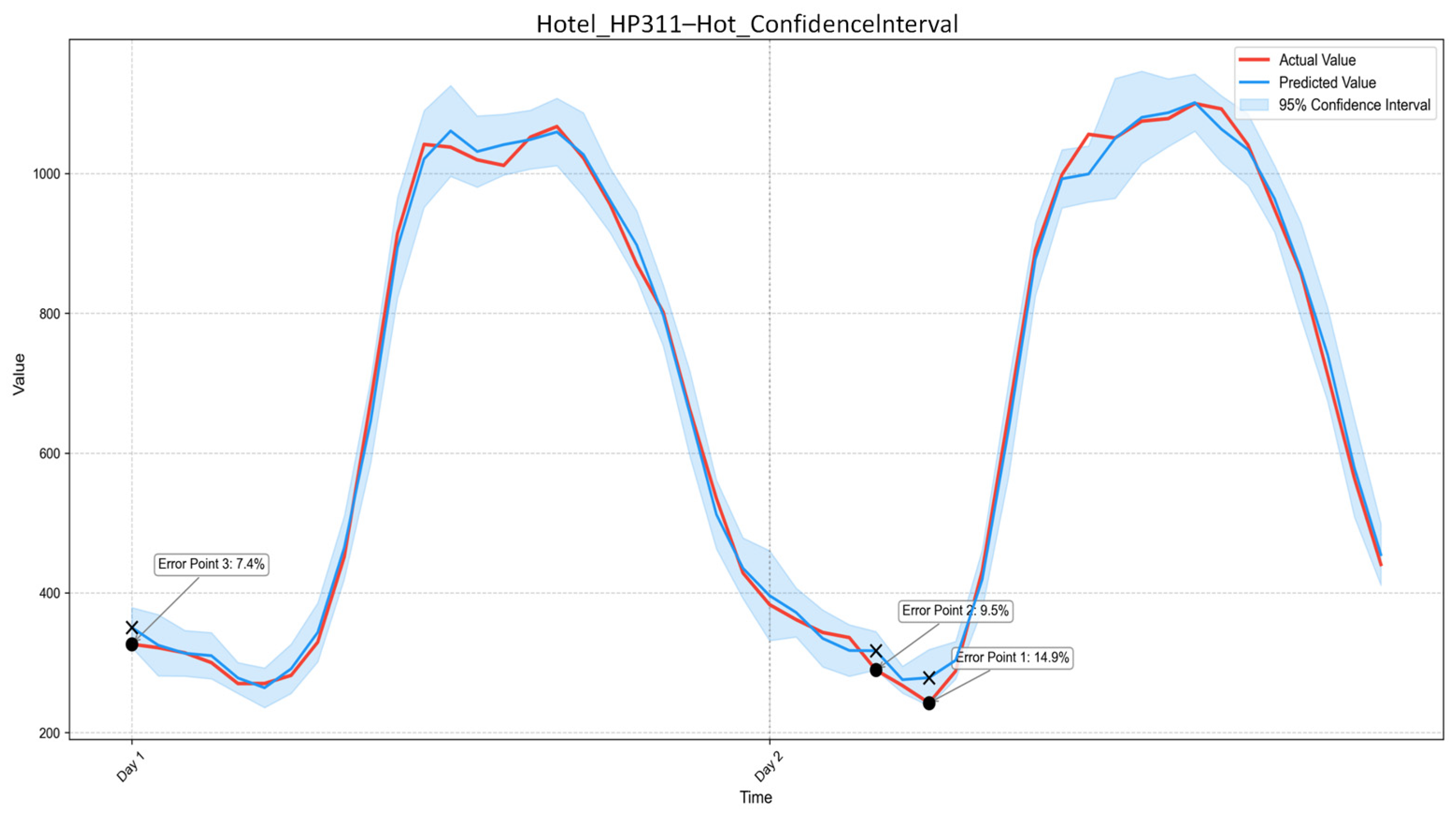
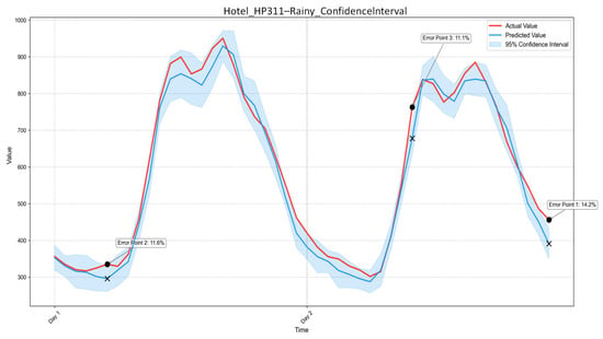
Figure A6.
Load curve with 95% confidence interval for Hotel_HP311--Rainy.
Figure A6.
Load curve with 95% confidence interval for Hotel_HP311--Rainy.

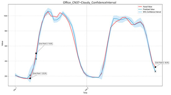
Figure A7.
Load curve with 95% confidence interval for Office_CN37-Cloudy.
Figure A7.
Load curve with 95% confidence interval for Office_CN37-Cloudy.
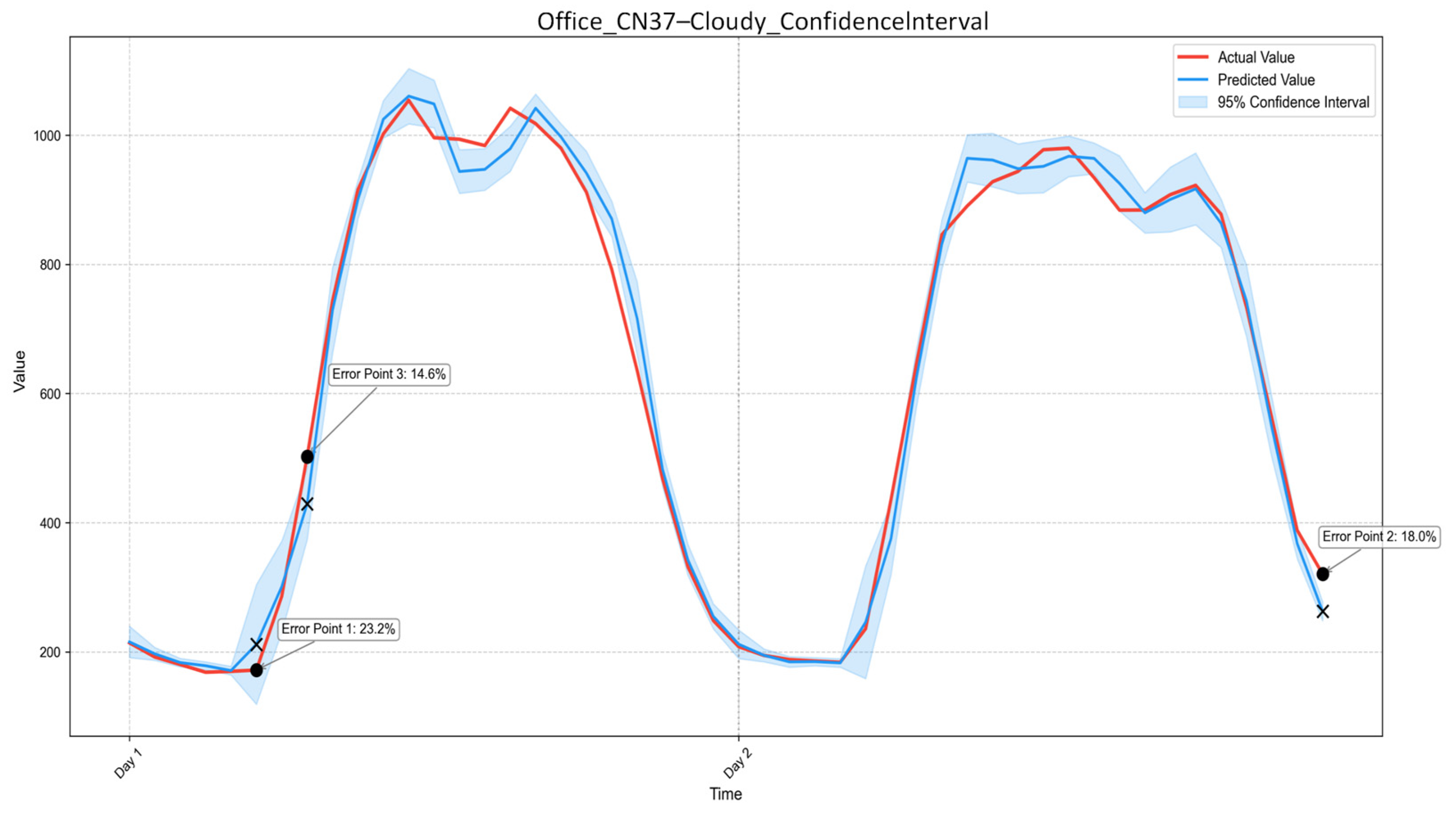
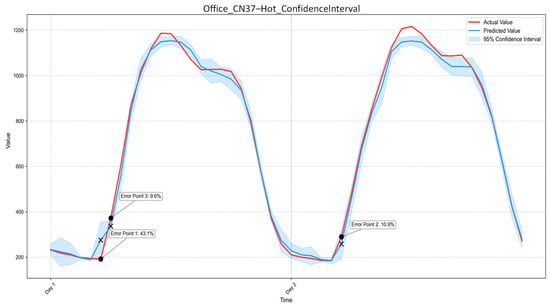
Figure A8.
Load curve with 95% confidence interval for Office_CN37-Hot.
Figure A8.
Load curve with 95% confidence interval for Office_CN37-Hot.
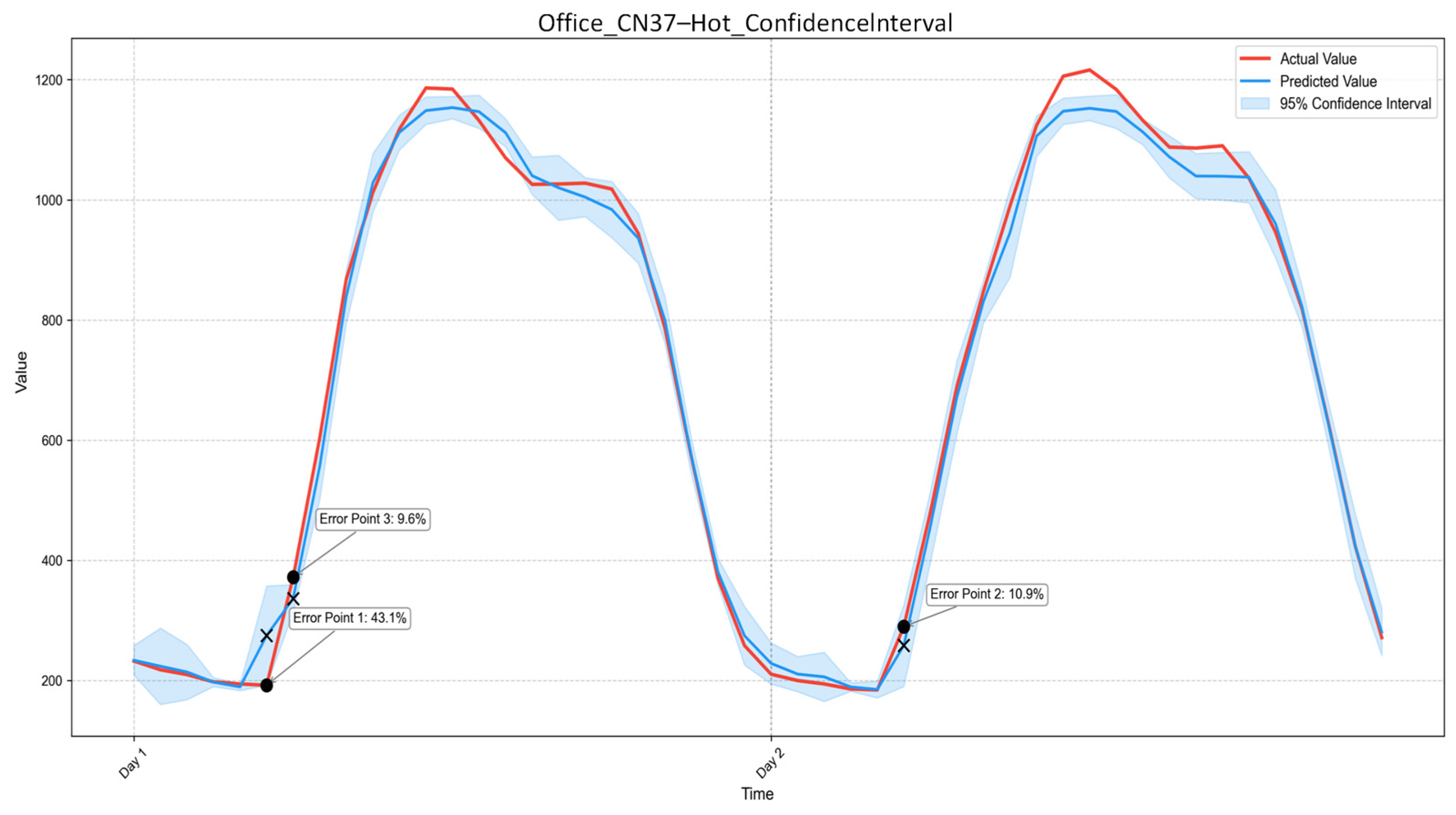
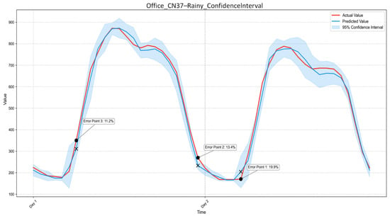
Figure A9.
Load curve with 95% confidence interval for Office_CN37-Rainy.
Figure A9.
Load curve with 95% confidence interval for Office_CN37-Rainy.

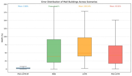
Figure A10.
Error boxplots of shopping mall buildings under multiple scenarios.
Figure A10.
Error boxplots of shopping mall buildings under multiple scenarios.

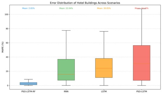
Figure A11.
Error boxplots of hotel buildings under multiple scenarios.
Figure A11.
Error boxplots of hotel buildings under multiple scenarios.
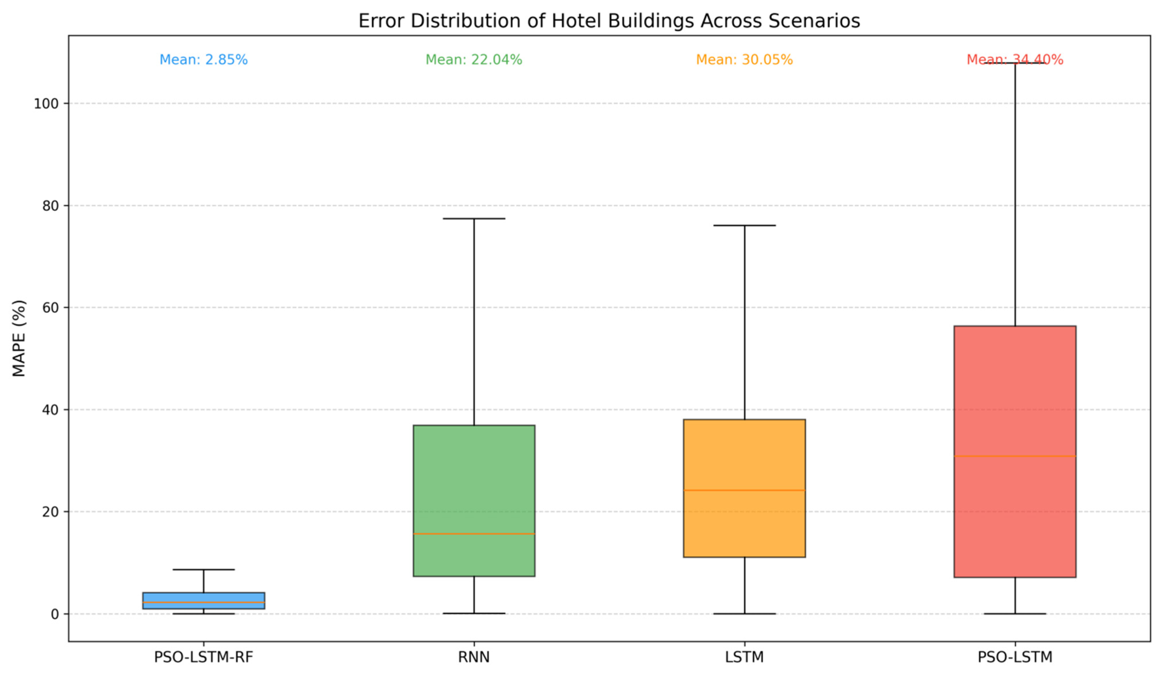
Figure A12.
Building load prediction under hot conditions.
Figure A12.
Building load prediction under hot conditions.
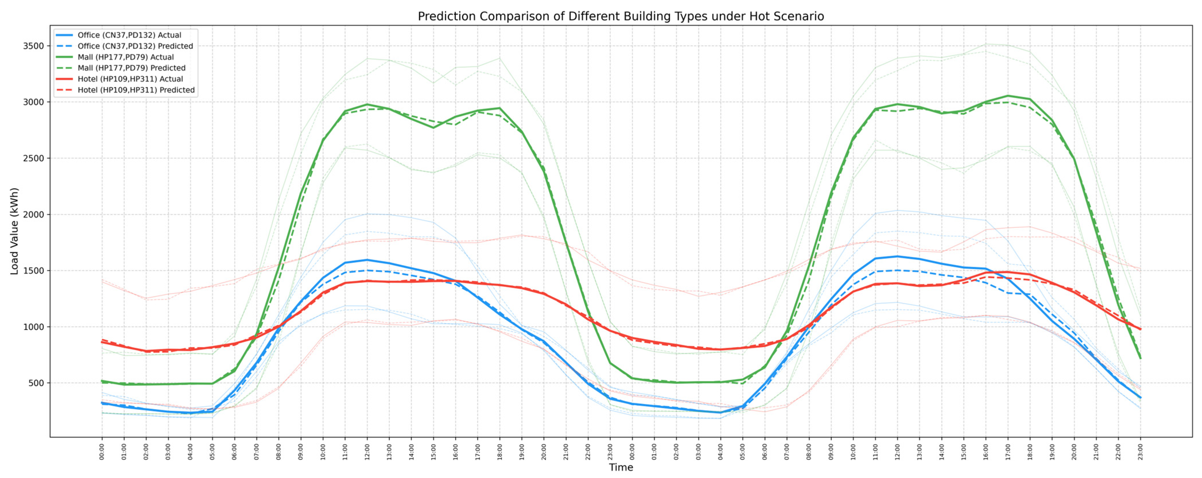
Figure A13.
Building load prediction under rainy conditions.
Figure A13.
Building load prediction under rainy conditions.
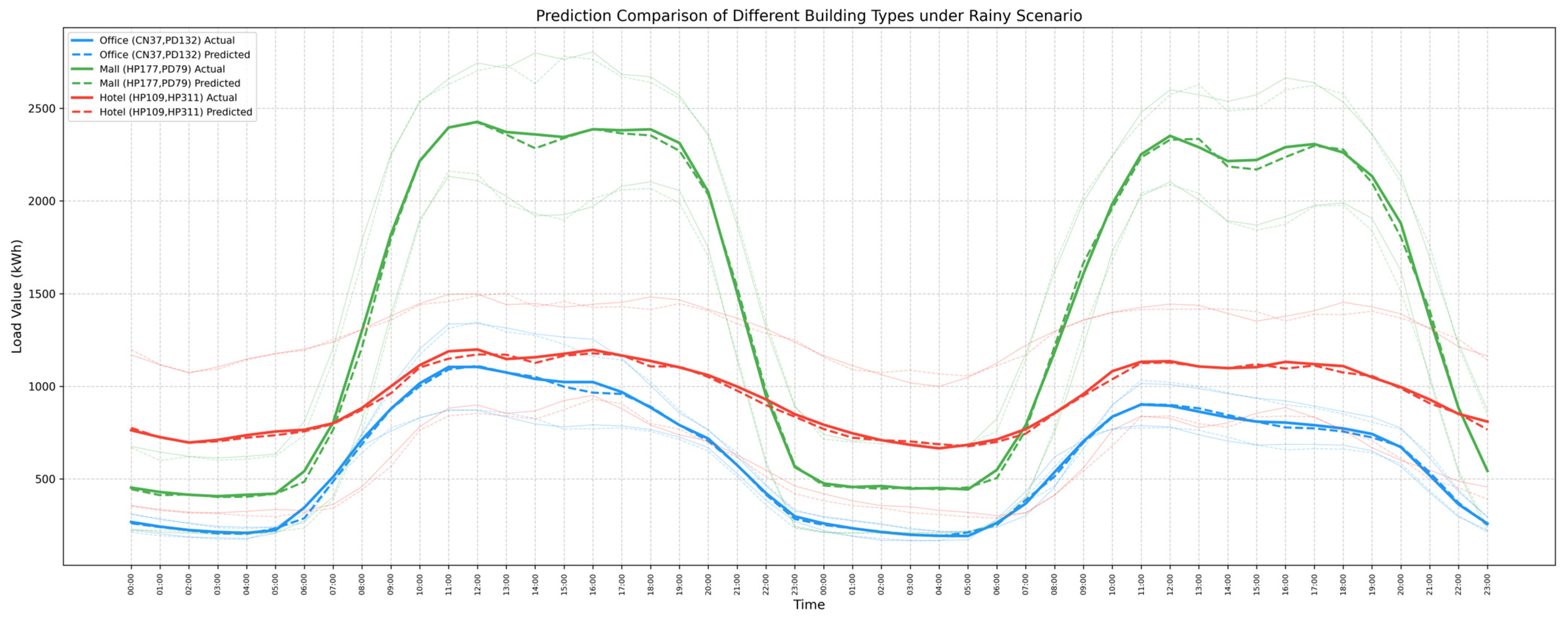
Figure A14.
Load profiles of shopping mall buildings under different scenarios.
Figure A14.
Load profiles of shopping mall buildings under different scenarios.
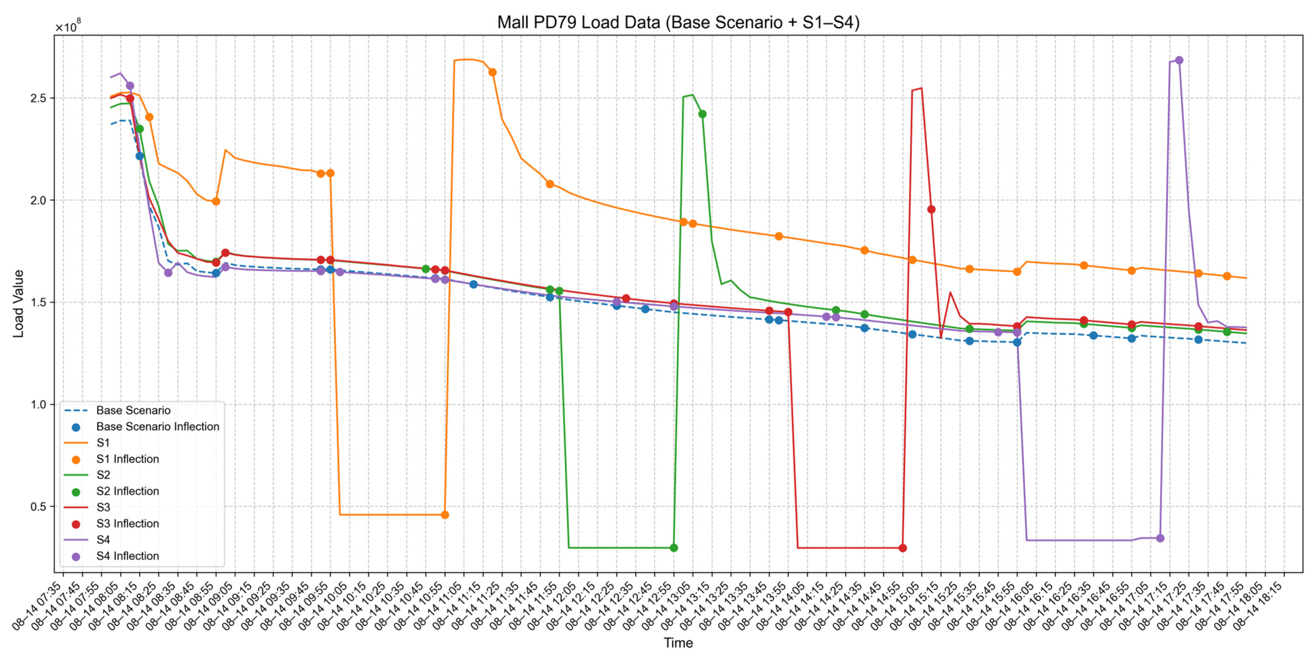
Figure A15.
Load profiles of hotel buildings under different scenarios.
Figure A15.
Load profiles of hotel buildings under different scenarios.
Appendix B

Table A1.
A Core hyperparameter description table of PSO-LSTM-RF model.
Table A1.
A Core hyperparameter description table of PSO-LSTM-RF model.
| Parameter Name | Definition | PSO Search Range | Optimal Value Distribution in 18 Groups of Experiments |
|---|---|---|---|
| Hidden Layer Dimension | Number of neurons in the hidden layer | 32~128 | 64~96 (12 groups), 32~50 (4 groups), 100~128 (2 groups) |
| Number of Hidden Layers | Number of stacked hidden layers | 1~3 | 1 layer (17 groups), 2 layers (1 group), 3 layers (0 groups) |
| Learning Rate | Parameter update step size | 0.0001~0.01 | 0.0001 (11 groups), 0.01 (7 groups) |
| Number of Decision Trees | Total number of integrated decision trees | 30~100 | 70~100 (15 groups), 50~69 (3 groups) |
| Maximum Tree Depth | Maximum depth of a single decision tree | 5~15 | 15 (12 groups), 10~14 (6 groups) |

Table A2.
Comparison of top 3 scores of similar days under different weight combinations.
Table A2.
Comparison of top 3 scores of similar days under different weight combinations.
| Weight Type | Top 1 Score | Top 2 Score | Top 3 Score |
|---|---|---|---|
| 0.9/0.1 | 0.94 | 0.93 | 0.92 |
| 0.8/0.2 | 0.87 | 0.85 | 0.85 |
| 0.5/0.5 | 0.82 | 0.81 | 0.81 |
| 0.2/0.8 | 0.78 | 0.75 | 0.74 |
| 0.1/0.9 | 0.76 | 0.73 | 0.72 |

Table A3.
Thermophysical properties of building envelope materials.
Table A3.
Thermophysical properties of building envelope materials.
| Material | Thermal Conductivity (W/(m·K)) | Density (kg/m3) | Specific Heat (J/(kg·K)) |
|---|---|---|---|
| Reinforced concrete | 1.74 | 2000 | 920 |
| Cement mortar | 0.93 | 1800 | 1050 |
| Extruded polystyrene foam | 0.03 | 35 | 1380 |
| Rock wool board | 0.041 | 120 | 1220 |
| Aerated concrete | 0.14 | 500 | 1050 |

Table A4.
Construction details of building envelopes.
Table A4.
Construction details of building envelopes.
| Structure | Composition | Main Thermal Parameter |
|---|---|---|
| Roof | Cement mortar (10 mm) | Overall heat transfer coefficient: 0.365 (W/(m2·K)) |
| Extruded polystyrene foam (75 mm) | ||
| Cement mortar (10 mm) | ||
| Reinforced concrete (120 mm) | ||
| Cement mortar (10 mm) | ||
| External wall | Cement mortar (15 mm) | Overall heat transfer coefficient: 0.451 (W/(m2·K)) |
| Rock wool board (40 mm) | ||
| Cement mortar (6 mm) | ||
| Aerated concrete (150 mm) | ||
| Floor | Rock wool board (30 mm) | Overall heat transfer coefficient: 1.119 (W/(m2·K)) |
| Window | 6 Low-E + 12 Air + 6 Clear glass | Overall heat transfer coefficient: 1.84 (W/(m2·K)) |

Table A5.
Comparison of model prediction errors for shopping mall buildings.
Table A5.
Comparison of model prediction errors for shopping mall buildings.
| Model | Mean Error (%) | Fluctuation (IQR) |
|---|---|---|
| PSO-LSTM-RF | 2.86 | 1.05 |
| RNN | 87.43 | 16.82 |
| LSTM | 100.14 | 18.75 |
| PSO-LSTM | 65.97 | 13.26 |

Table A6.
Comparison of model prediction errors for hotel buildings.
Table A6.
Comparison of model prediction errors for hotel buildings.
| Model | Mean Error (%) | Fluctuation (IQR) |
|---|---|---|
| PSO-LSTM-RF | 2.69 | 0.98 |
| RNN | 22.04 | 5.73 |
| LSTM | 30.05 | 6.89 |
| PSO-LSTM | 56.62 | 11.23 |

Table A7.
Evaluation of BAM for shopping mall buildings across scenarios.
Table A7.
Evaluation of BAM for shopping mall buildings across scenarios.
| Scenario | S1 | S2 | S3 | S4 |
|---|---|---|---|---|
| Building adjustable margin (kWh) | 446.12 | 394.60 | 361.22 | 417.45 |
| Response duration (min) | 60 | 60 | 60 | 75 |

Table A8.
Evaluation of BAM for hotel buildings across scenarios.
Table A8.
Evaluation of BAM for hotel buildings across scenarios.
| Scenario | S1 | S2 | S3 | S4 |
|---|---|---|---|---|
| Adjustable margin (kWh) | 526.88 | 579.27 | 463.44 | 393.01 |
| Response duration (min) | 120 | 135 | 105 | 85 |
References
- United Nations Environment Programme and Global Alliance for Buildings and Construction. Not Just Another Brick in the Wall: The Solutions Exist—Scaling Them Will Build on Progress and Cut Emissions Fast. Global Status Report for Buildings and Construction 2024/2025; Knowledge Repository-UNEP, UNEP: Nairobi, Kenya, 2025; Available online: https://wedocs.unep.org/20.500.11822/47214 (accessed on 15 July 2025).
- Luo, Z.Y.; Peng, J.Q.; Hu, M.M. Multi-Objective Optimal Dispatch of Household Flexible Loads Based on Their Real-Life Operating Characteristics and Energy-Related Occupant Behavior. Build. Simul. 2023, 16, 2005–2025. [Google Scholar] [CrossRef]
- Arteconi, A.; Mugnini, A.; Polonara, F. Energy Flexible Buildings: A Methodology for Rating the Flexibility Performance of Buildings with Electric Heating and Cooling Systems. Appl. Energy 2019, 251, 113387. [Google Scholar] [CrossRef]
- Khatoon, S.; Shah, A.N. Prediction of Comfort Parameters for Naturally Ventilated Underground Car Parks. Nucleus 2016, 53, 214–220. [Google Scholar] [CrossRef]
- Tarsitano, A.; Amerise, I.L. Short-Term Load Forecasting Using a Two-Stage sarimax model. Energy 2017, 133, 108–114. [Google Scholar] [CrossRef]
- Huang, Y.Y.; Yu, C.; Huang, W.X.; Qin, Z.; Bi, L.; Yang, L. Building Load Forecasting Based on Sensor Network and Gaussian Process Regression. Mod. Electr. Power 2021, 38, 664–673. [Google Scholar]
- Li, B.; Lu, M.Z. Short-term load forecasting modeling of regional power grid considering real-time meteorological coupling effect. Autom. Electr. Power Syst. 2020, 44, 60–68. [Google Scholar]
- Li, X.; Li, C.; Cong, L.; Ren, Z.; Luo, H.; Wang, Y.; Yuan, H.; Qiu, H. Short-term load forecasting based on dynamic weight similar day selection algorithm. Power Syst. Prot. Control 2017, 45, 1–8. [Google Scholar]
- Sun, W.; Hao, Z.; Zhao, X. Load characteristics analysis and short term load forecasting research of a county power grid. North China Electr. Power 2017, 27–31. [Google Scholar] [CrossRef]
- Li, A.; Xiao, F.; Fan, C.; Hu, M. Development of an ANN-Based Building Energy Model for Information-Poor Buildings Using Transfer Learning. Build. Simul. 2021, 14, 89–101. [Google Scholar] [CrossRef]
- Wang, X. Power System Short-Term Load Forecasting Based on BP Neural Network. J. Phys.: Conf. Ser. 2022, 2378, 012068. [Google Scholar] [CrossRef]
- Luo, R.X.; Liu, S.M.; You, M.N.; Lin, J.C. Load Forecasting Based on Weighted Grey Relational Degree and Improved ABC-SVM. J. Electr. Eng. Technol. 2021, 16, 2191–2200. [Google Scholar] [CrossRef]
- Tang, R.; Fan, C.; Zeng, F.Z.; Feng, W. Data-Driven Model Predictive Control for Power Demand Management and Fast Demand Response of Commercial Buildings Using Support Vector Regression. Build. Simul. 2022, 15, 317–331. [Google Scholar] [CrossRef]
- Wang, Z.; Wang, Y.; Zeng, R.; Srinivasan, R.S.; Ahrentzen, S. Random Forest Based Hourly Building Energy Prediction. Energy Build. 2018, 171, 11–25. [Google Scholar] [CrossRef]
- Sala, J.; Li, R.L.; Christensen, M.H. Clustering and Classification of Energy Meter Data: A Comparison Analysis of Data from Individual Homes and the Aggregated Data from Multiple Homes. Build. Simul. 2021, 14, 103–117. [Google Scholar] [CrossRef]
- Jang, J.; Han, I.; Leigh, S.B. Prediction of Heating Energy Consumption with Operation Pattern Variables for Non-Residential Buildings Using LSTM Networks. Energy Build. 2022, 255, 111647. [Google Scholar] [CrossRef]
- Fang, L.; He, B. A Deep Learning Framework Using Multi-Feature Fusion Recurrent Neural Networks for Energy Consumption Forecasting. Appl. Energy 2023, 348, 121563. [Google Scholar] [CrossRef]
- Rahman, A.; Srikumar, V.; Smith, A.D. Predicting Electricity Consumption for Commercial and Residential Buildings Using Deep Recurrent Neural Networks. Appl. Energy 2018, 212, 372–385. [Google Scholar] [CrossRef]
- Shu, X.; Zhang, L.; Qi, G.J.; Liu, W.; Tang, J. Spatiotemporal Co-Attention Recurrent Neural Networks for Human-Skeleton Motion Prediction. IEEE Trans. Pattern Anal. Mach. Intell. 2022, 44, 3300–3315. [Google Scholar] [CrossRef]
- Ni, L.; Wang, D.; Singh, V.P.; Wu, J.; Yang, Y.; Tao, Y.; Zhang, J. Streamflow and Rainfall Forecasting by Two Long Short-Term Memory-Based Models. J. Hydrol. 2020, 583, 124296. [Google Scholar] [CrossRef]
- Zhou, C.; Fang, Z.; Xu, X.; Zhang, X.; Ding, Y.; Jiang, X. Using Long Short-Term Memory Networks to Predict Energy Consumption of Air-Conditioning Systems. Sustain. Cities Soc. 2020, 55, 102000. [Google Scholar] [CrossRef]
- Sundaram, K.; Preethaa, K.R.S.; Natarajan, Y.; Muthuramalingam, A.; Ali, A.A.Y. Advancing Building Energy Efficiency: A Deep Learning Approach to Early-Stage Prediction of Residential Electric Consumption. Energy Rep. 2024, 12, 1281–1292. [Google Scholar] [CrossRef]
- Li, W.; Jiang, X. Prediction of Air Pollutant Concentrations Based on TCN-BiLSTM-DMAttention with STL Decomposition. Sci. Rep. 2023, 13, 4665. [Google Scholar] [CrossRef]
- Ewees, A.A.; Al-ganess, M.A.A.; Abualigah, L.; Abd Elaziz, M. HBO-LSTM: Optimized Long Short Term Memory with Heap-Based Optimizer for Wind Power Forecasting. Energy Convers. Manag. 2022, 268, 116022. [Google Scholar] [CrossRef]
- Luo, X.; Shi, W. Optimal Regulation of Flexible Loads in Rural Residential Buildings Considering Mobile Batteries: A Case Study in Shaanxi Province. Build. Simul. 2024, 17, 1065–1083. [Google Scholar] [CrossRef]
- Zhu, J.; Tian, Z.; Niu, J.; Lu, Y.; Cheng, B.; Zhou, H. Machine Learning-Enhanced Lightweight Rule-Based Control Strategy for Building Energy Demand Response. Build. Simul. 2025, 18, 1857–1876. [Google Scholar] [CrossRef]
- Dai, M.; Li, H.; Wang, S. Multi-Agent Based Distributed Cooperative Control of Air-Conditioning Systems for Building Fast Demand Response. J. Build. Eng. 2023, 77, 107463. [Google Scholar] [CrossRef]
- Dai, M.; Li, H.; Li, X.; Wang, S. Reconfigurable Supply-Based Feedback Control for Enhanced Energy Flexibility of Air-Conditioning Systems Facilitating Grid-Interactive Buildings. Adv. Appl. Energy 2024, 14, 100176. [Google Scholar] [CrossRef]
- Yin, R.; Kara, E.C.; Li, Y.; DeForest, N.; Wang, K.; Yong, T.; Stadler, M. Quantifying Flexibility of Commercial and Residential Loads for Demand Response Using Setpoint Changes. Adv. Appl. Energy 2016, 177, 149–164. [Google Scholar] [CrossRef]
- Ding, Y.; Liu, Y.; Wang, Q.; Liu, L.; Tian, Z. Flexibility potential quantification and regulation measure comparison for the building air-conditioning system. J. Clean. Prod. 2024, 434, 140086. [Google Scholar] [CrossRef]
- Ruan, Y.; Ma, J.; Meng, H.; Qian, F.; Xu, T.; Yao, J. Potential quantification and impact factors analysis of energy flexibility in residential buildings with preheating control strategies. J. Build. Eng. 2023, 78, 107657. [Google Scholar] [CrossRef]
- Han, B.; Li, H.; Wang, S. A probabilistic model for real-time quantification of building energy flexibility. Adv. Appl. Energy 2024, 15, 100186. [Google Scholar] [CrossRef]
- Zhu, J.; Niu, J.; Tian, Z.; Zhou, R.; Ye, C. Rapid quantification of demand response potential of building HAVC system via data-driven model. Appl. Energy 2022, 325, 119796. [Google Scholar] [CrossRef]
- GB 55015-2021; General Code for Energy Efficiency and Renewable Energy Application in Buildings. Ministry of Housing and Urban-Rural Development of the People’s Republic of China: Beijing, China, 2021.
Disclaimer/Publisher’s Note: The statements, opinions and data contained in all publications are solely those of the individual author(s) and contributor(s) and not of MDPI and/or the editor(s). MDPI and/or the editor(s) disclaim responsibility for any injury to people or property resulting from any ideas, methods, instructions or products referred to in the content. |
© 2025 by the authors. Licensee MDPI, Basel, Switzerland. This article is an open access article distributed under the terms and conditions of the Creative Commons Attribution (CC BY) license.

