A Reinforcement Learning Guided Oppositional Mountain Gazelle Optimizer for Time–Cost–Risk Trade-Off Optimization Problems

Abstract

Existing metaheuristic approaches often struggle to maintain an effective exploration–exploitation balance and are prone to premature convergence when addressing highly conflicting time–cost–safety–risk trade-off problems (TCSRTPs) under complex construction project constraints, which can adversely affect project productivity, safety, and the provision of decent jobs in the construction sector. To overcome these limitations, this study introduces a hybrid metaheuristic called the Q-Learning Inspired Mountain Gazelle Optimizer (QL-MGO) for solving multi-objective TCSRTPs in construction project management, supporting the delivery of resilient infrastructure and resilient building projects. QL-MGO enhances the original MGO by integrating Q-learning with an opposition-based learning strategy to improve the balance between exploration and exploitation while reducing computational effort and enhancing resource efficiency in construction scheduling. Each gazelle functions as an adaptive agent that learns effective search behaviors through a state–action–reward structure, thereby strengthening convergence stability and preserving solution diversity. A dynamic switching mechanism represents the core innovation of the proposed approach, enabling Q-learning to determine when opposition-based learning should be applied based on the performance history of the search process. The performance of QL-MGO is evaluated using 18- and 37-activity construction scheduling problems and compared with NDSII-MGO, NDSII-Jaya, NDSII-TLBO, the multi-objective genetic algorithm (MOGA), and NDSII-Rao-2. The results demonstrate that QL-MGO consistently generates superior Pareto fronts. For the 18-activity project, QL-MGO achieves the highest hypervolume (HV) value of 0.945 with a spread of 0.821, outperforming NDSII-Rao-2, MOGA, and NDSII-MGO. Similar results are observed for the 37-activity project, where QL-MGO attains the highest HV of 0.899 with a spread of 0.674, exceeding the performance of NDSII-Jaya, NDSII-TLBO, and NDSII-MGO. Overall, the integration of Q-learning significantly enhances the search capability of MGO, resulting in faster convergence, improved solution diversity, and more reliable multi-objective trade-off solutions. QL-MGO therefore serves as an effective and computationally efficient decision-support tool for construction scheduling that promotes safer, more reliable, and resource-efficient project delivery.

1. Introduction

Construction project management is an inherently complex process shaped by dynamic conditions, diverse stakeholders, and multiple, often conflicting, performance objectives. Traditionally, project success is assessed through the constraints of time, cost, and quality, commonly referred to as the triple constraint [1]. In contemporary practice, however, this framework is frequently expanded to include risk as an equally important and interrelated dimension. Efforts to shorten project duration or reduce overall costs often increase exposure to uncertainties and negative outcomes, which leads to the well-known time–cost–safety risk trade off problem (TCSRTPs) [2]. Managing these interrelated factors is not only an operational requirement but also a strategic necessity for ensuring project success, improving client satisfaction, and strengthening organizational competitiveness and profitability.

The time–cost–risk trade off problem aims to determine a set of efficient project execution plans in which none of the objectives, namely time, cost, or risk, can be improved without causing a decline in at least one of the others. This collection of equally efficient alternatives forms what is known as the Pareto optimal front [3]. Earlier optimization approaches, including linear programming and dynamic programming, were mainly applied to simpler versions of the problem such as the traditional time–cost trade off. These methods, however, are unable to cope with the significant computational challenges created by the non-linear behavior of risk and the large discrete search spaces that characterize construction projects in practice [4,5,6,7].

To overcome these challenges, metaheuristic algorithms have gained prominence as effective methods for addressing complex multi-objective optimization problems. Approaches such as Genetic Algorithms, Particle Swarm Optimization (PSO), and Simulated Annealing have been widely used to approximate the Pareto optimal front for the time–cost–risk trade off problem [8]. These population based algorithms are particularly effective at exploring large search domains and avoiding entrapment in local optima. Nevertheless, their performance is often influenced by the need to properly adjust algorithm specific parameters, such as crossover and mutation settings in Genetic Algorithms or inertia weight in PSO [5]. This tuning process is difficult and can substantially affect both the quality of the solutions and the speed of convergence [9].

Kumar et al. [10] developed a time–cost trade-off optimization model specifically designed for Indian highway construction projects. The model applies the NSGA-II algorithm to minimize both project duration and cost simultaneously, while accounting for essential constraints such as activity precedence and resource limitations. Their findings show that NSGA-II surpasses conventional techniques by generating a wide range of Pareto-optimal solutions. To determine the most appropriate option from the Pareto front, the weighted sum approach was used, underscoring the effectiveness of the algorithm in tackling complex Indian construction scenarios.

Similarly, Pham et al. [11] proposed an enhanced method by integrating the multi-verse optimizer (MVO) with OBL to solve TCTP in large-scale construction projects. The improved algorithm, named iMVO, was evaluated on networks containing 18 to 290 activities. Results demonstrated that iMVO consistently delivers superior outcomes, outperforming earlier approaches in terms of both mean deviation percentage and computational efficiency.

Researchers have increasingly turned to optimization techniques, particularly hybrid approaches, to address complex engineering challenges and achieve more efficient and reliable outcomes [12,13,14,15,16,17]. Earlier works predominantly employed randomization techniques to generate the initial population. However, prior work has highlighted that starting the optimization process with higher-quality candidate solutions can significantly accelerate convergence and improve search efficiency [18,19]. To this end, strategies such as Opposition-Based Learning [20], as well as Q-learning [21], have been proposed. OBL evaluates a candidate solution together with its opposite under the premise that the opposite point may be closer to the global optimum than a randomly generated solution [22].

A major direction for improving metaheuristic algorithms is the incorporation of reinforcement learning. Reinforcement learning, a sub-field of machine learning, enables an agent to interact with its environment and learn effective decision-making strategies by maximizing cumulative rewards [23,24]. Recent advances in reinforcement learning that utilize structural information aim to enhance sample efficiency, accelerate convergence, and refine exploration behavior by embedding informative structural elements into the learning process [25,26].

Although the Mountain Gazelle Optimizer (MGO) is widely utilized in academic research, its performance can still be enhanced by incorporating mechanisms that improve convergence speed and solution quality. In addition, the broader research challenge involves examining the strengths and limitations of metaheuristic algorithms and increasing their effectiveness through the introduction of novel or modified strategies. For example, Li et al. [27] proposed DERLFR, a reinforcement learning–enhanced differential evolution method that integrates Q-learning and fitness-based ranking, where each individual in the population functions as an agent with hierarchical state variables determined by fitness levels. Similarly, Samma et al. [28] developed an RL-driven variant of Particle Swarm Optimization known as RLMPSO.

With the evolution of project management methodologies, safety risk has become as essential as time and cost, giving rise to multi-objective time–cost–safety risk trade-off (TCSRTP) optimization models. Early contributions include the qualitative, activity-based safety risk framework of Afshar and Dolabi [29] combined with genetic algorithms. Subsequent studies have adopted hybrid and advanced metaheuristics, such as artificial bee colony algorithms with differential evolution [30], NSGA-III [31], particle swarm optimization [32], and adaptive opposition-based slime mold algorithms [33]. Solving TCSRTP problems demands the generation of a diverse set of Pareto-optimal solutions, a task that becomes increasingly difficult as the number of objectives grows [3]. To maintain diversity, non-dominated sorting combined with crowding distance techniques has been widely applied. Against this backdrop, the MGO, originally introduced by Abdollahzadeh et al. [9], represents a promising alternative for addressing TCSRTPs in construction scheduling.

Recent studies have explored decision-making and ranking-based techniques, such as Grey Relational Analysis (GRA), to address complex geotechnical and construction-related optimization problems. For instance, Asadoullahtabar et al. [34] employed a GRA-based framework to systematically evaluate and prioritize multiple conflicting criteria under uncertainty, demonstrating its effectiveness in engineering geology applications. While GRA-based approaches provide structured multi-criteria assessment and interpretability, they are generally static in nature and do not incorporate adaptive learning during the optimization process. In contrast, the proposed QL-MGO adopts a learning-driven evolutionary search mechanism, where Q-learning dynamically regulates exploration–exploitation behavior and opposition-based learning enhances population diversity. This enables QL-MGO to continuously adapt its search strategy during optimization, making it more suitable for solving highly non-linear and dynamic multi-objective TCSRTPs.

The classical MGO balances exploration and exploitation; however, it can suffer from premature convergence or insufficient diversity when applied to complex multi-objective problems. Motivated by these limitations, the proposed Q-Learning Inspired Mountain Gazelle Optimizer (QL-MGO) integrates Q-learning to adaptively guide search agents between exploration and exploitation based on past experiences, thereby improving search intelligence and convergence performance. In addition, OBL is incorporated to generate opposite candidate solutions, enhancing diversity and mitigating the risk of premature convergence. By combining Q-learning with OBL, QL-MGO provides a robust and computationally efficient approach for multi-objective optimization, capable of generating high-quality Pareto-optimal solutions and supporting better decision-making in complex problems such as construction project TCSRTPs.

The underlying learning-based approach has previously been demonstrated to be effective on mathematical benchmark problems in Ref. [35]. Building on this foundation, the present study extends the approach to address TCSRT optimization problems. The algorithm’s effectiveness is assessed using widely accepted multi-objective performance indicators, including Hypervolume (HV) for convergence and diversity, and Spread (Sp) for Pareto front distribution uniformity. Additionally, correlation analysis is conducted to examine the trade-offs among time, cost, and safety risk. The proposed QL-MGO is evaluated on two construction projects involving 18 and 37 activities, demonstrating superior performance compared to state-of-the-art comparison algorithms. The main contributions of this study are summarized as follows:

• A Q-learning–assisted Mountain Gazelle Optimizer incorporating opposition-based learning (OBL), termed QL-MGO, is developed to enable adaptive transitions between exploration and exploitation phases.
• The integration of Q-learning enhances the search efficiency and solution diversity of MGO while reducing the likelihood of premature convergence.
• The proposed QL-MGO is validated using two time–cost–safety–risk trade-off scheduling problems.
• A comprehensive comparative analysis of QL-MGO, the conventional MGO, and other benchmark algorithms is conducted using performance indicators including the number of function evaluations (NFE), hypervolume (HV), and spread (Sp).

The remainder of this paper is organized as follows: first, the mathematical formulation of the TCTP is presented. This is followed by the description of the Q-learning-enhanced MGO algorithm as the solution methodology. Next, the influence of OBL-based initialization on optimization efficiency in TCTP is analyzed. Finally, the empirical results are discussed and the main conclusions are summarized.

2. Mathematical Formulation of TCSRT

The TCSRT problem in project management is a multi-objective optimization problem that aims to simultaneously minimize project time, cost, and risk in project execution. It involves selecting appropriate execution modes for each project activity from available alternatives as follows [36]:

$$minimize \sum _{j=1}^S\sum _{k=1}^{m\left(j\right)}({dc}_{jk} x_{jk})+D\times ic$$

(1)

This is subject to the following:

$$\sum _{k=1}^{m\left(j\right)}{x}_{jk}=1, \forall j=1, \dots , S$$

(2)

$$\sum _{k=1}^{m\left(j\right)}{d}_{jk} x_{jk}+{St}_j\le {St}_l, \forall l\in {Sc}_j and \forall j=1, \dots , S$$

(3)

$$D \ge {St}_{S+1} \forall l\in {Sc}_j and \forall j=1, \dots , S$$

(4)

where ${dc}_{jk}$ shows the direct cost of option k for activity j; $x_{jk}$ is a 0–1 index variable which is equal to 1 if option k is chosen for executing activity j, and 0 otherwise; ic is the indirect cost rate of the project; D is the total project duration; $d_{jk}$ is the duration of activity j for option k; ${St}_j$ is the start time for activity j; and ${Sc}_j$ is the set of immediate successors for activity j.

The project safety risk is calculated by summing the products of the likelihood and severity of all selected execution modes across activities, representing the third objective in this multi-objective optimization framework [37]. Formally,

$$\mathrm{Minimize} \mathrm{SR}={\displaystyle {\sum }_{i=1}^n}{\displaystyle {\sum }_{j=1}^{m_i}}{RL}_{ij} \ast {RS}_{ij}$$

(5)

where RL_ij represents the risk likelihood and severity associated with the j-th execution mode of the i-th activity, respectively, and SR is the total project safety risk [37].

In this study, time, cost, and safety risk are treated as the three primary objectives. The decision variables correspond to the selection of execution modes for each activity, with lower bounds set to 1 and upper bounds equal to the number of available options per activity. The Critical Path Method (CPM) is employed to define activity dependencies, ensuring that subsequent tasks commence only after the completion of their predecessors.

The main constraints include the following:

• A single execution mode must be selected for each activity.
• All activities must be completed while respecting precedence relationships.
• Each activity’s execution mode must satisfy the defined lower and upper bound limits.

3. The Methodology Map

3.1. Mountain Gazelle Optimizer (MGO)

The MGO is a recently developed nature-inspired metaheuristic that models the adaptive foraging, social interaction, and predator-avoidance behaviors of mountain gazelles. By simulating these movements in response to environmental cues, the algorithm guides the search process through coordinated phases that maintain an effective balance between exploration and exploitation for solving complex optimization problems (Abdollahzadeh et al. [9]). The mathematical formulations are as follows:

Let X(t) = [x₁(t), x₂(t),…, x_N(t)] represent a population of N gazelles at iteration t, each gazelle corresponding to a candidate solution in a D-dimensional search space.

3.1.1. Initialization

The initial population is randomly generated within the given search boundaries:

x_i,j(0) = b_l + r_j × (b_u − b_l)

(6)

where b_l and b_u are the lower and upper bounds of the search space, and r_j ∈ [0, 1] is a uniformly distributed random number.

Such an approach fundamentally alters the behavior of the update strategies, including territorial solitary males $\left(TSMs\right)$, maternity herds $\left(MHs\right)$, and bachelor male herds $\left(BMHs\right)$, which are reformulated as Equations (7)–(10) to accommodate the variability introduced by chaos-based dynamics. The migration to search for food $\left(MSF\right)$ mechanism, however, remains unchanged as in the original MGO as Equation (7).

3.1.2. Behavioral Phases

The MGO defines four key behavioral mechanisms derived from Abdollahzadeh et al. [9]:

(a) 

Territorial Solitary Male (TSM) Behavior

This phase simulates dominant male gazelles defending their territory while searching for better positions:

$$TSM={male}_{gazelle}-\left|\left({ri}_1\times BH-{ri}_2\times X\left(t\right)\right)\times F\right|$$

(7)

where

• ${male}_{gazelle}$: the position of the dominant male gazelle (best solution),
• BH: the best herd (elite position),
• X(t): current gazelle position,
• F: a control factor that balances exploration and exploitation,
• r₁, r₂ ∈ [0, 1] random coefficients.

(b) 

Maternity Herd (MH) Behavior

This phase models female gazelles moving in coordination for protection and resource gathering:

$$MH=BH+\left({ri}_3\times {male}_{gazelle}-{ri}_4\times X_{rand}\right)$$

(8)

where

• X_rand: a randomly selected gazelle,
• r₃, r₄ ∈ [0, 1] random coefficients.

This stage enhances exploration by moving toward the best herd while maintaining stochastic diversity.

(c) 

Bachelor Male Herd (BMH) Behavior

This phase represents less dominant males that roam widely to search for new territories or herds:

$$BMH=\left(X\left(t\right)-D\right)+\left({ri}_5\times {male}_{gazelle}-{ri}_6\times BH\right)$$

(9)

where, D: a distance control parameter that defines the movement radius, and r₅, r₆ ∈ [0, 1] random numbers.

This phase increases diversification and helps prevent premature convergence.

(d) 

Migration to Search for Food (MSF)

Migration allows gazelles to explore new regions of the search space:

$$MSF=\left(b_u-b_l\right)\times r_7+b_l$$

(10)

where

• $r_7$ ∈ [0, 1]: random scalar controlling the exploration step.

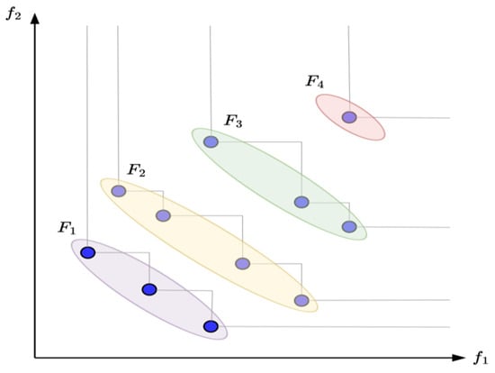
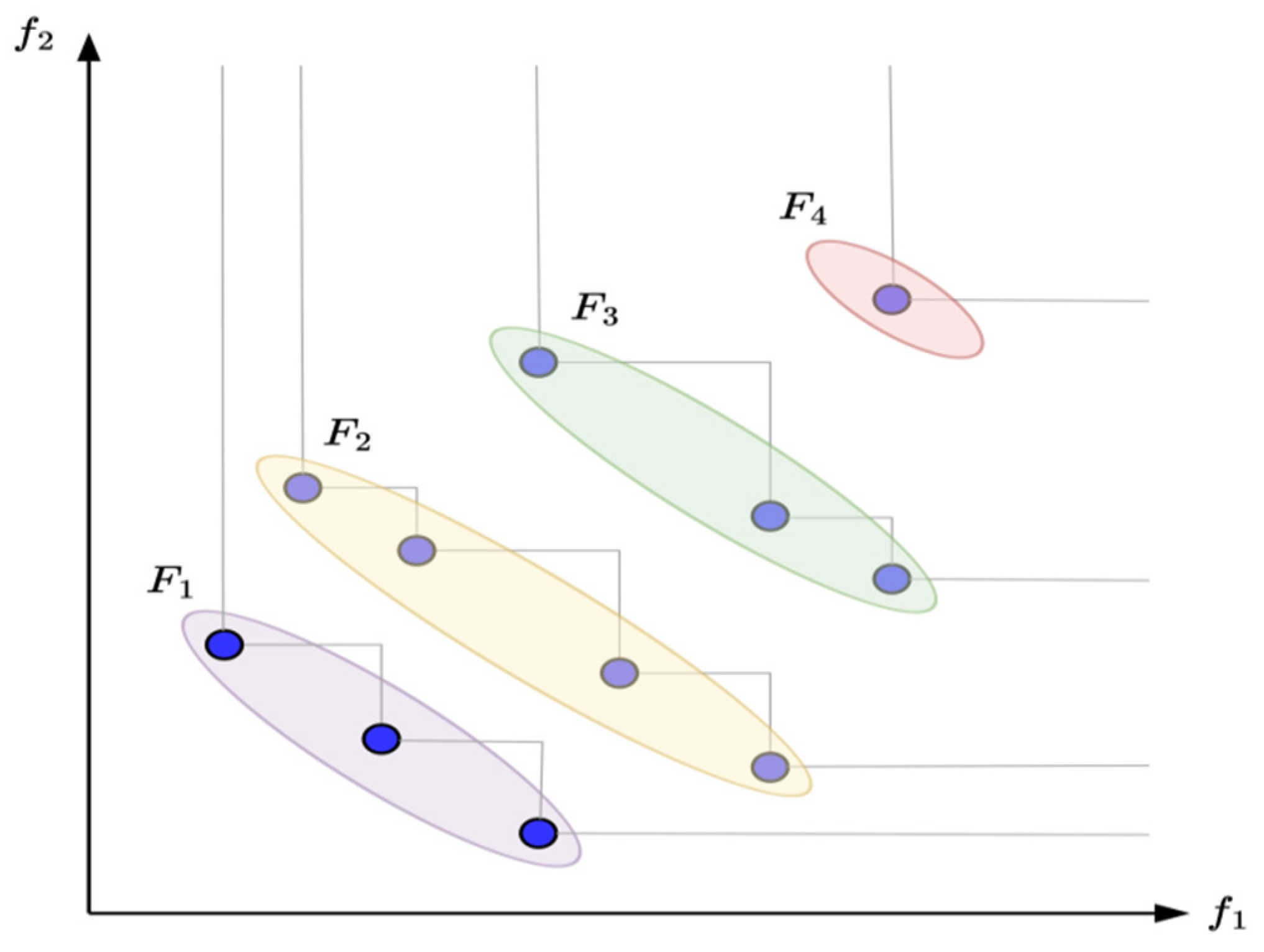
To effectively address the multi-objective nature of optimization problems, this study incorporates a non-dominated sorting (NDS, [3]) mechanism into the MGO for solution ranking. NDS, a fundamental component of Pareto-based multi-objective optimization, classifies individuals into different Pareto fronts based on dominance relationships (see Figure 1).

Figure 1. Non-dominated solution mechanism.

Specifically, the figure shows four Pareto fronts labeled F₁, F₂, F₃, and F₄, each representing a set of non-dominated solutions for objectives f₁ and f₂. Each front F_i contains multiple candidate solutions (dots) that are mutually non-dominated within the front. The steps represented by the fronts indicate the progression of the optimization process:

• F₁: Initial Pareto front obtained from the first iteration.
• F₂: Updated front showing improved trade-offs after the second iteration.
• F₃: Further refinement of non-dominated solutions.
• F₄: Final Pareto front representing the best trade-offs between f₁ and f₂ identified by the algorithm.

This figure visually explains how the algorithm iteratively improves solution quality and diversity across multiple iterations, according to Equations (11) and (12).

∀v ∈ {1, 2, …, V}: fv (x₁) ≤ fv (x₂)

(11)

∀u ∈ {1, 2, …, V}: fu (x₁) ≤ fu (x₂)

(12)

The NDS process begins by evaluating each individual in the population to determine two attributes: the number of individuals that dominate it (n_p) and the set of individuals it dominates (S_p). Individuals with n_p equal to zero, meaning they are not dominated by any other population members, are assigned to the first Pareto front F₁. Subsequent fronts F₂, F₃, and so on are constructed iteratively [3].

3.2. Population Selection Procedure

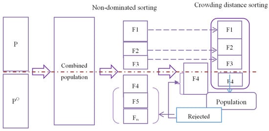
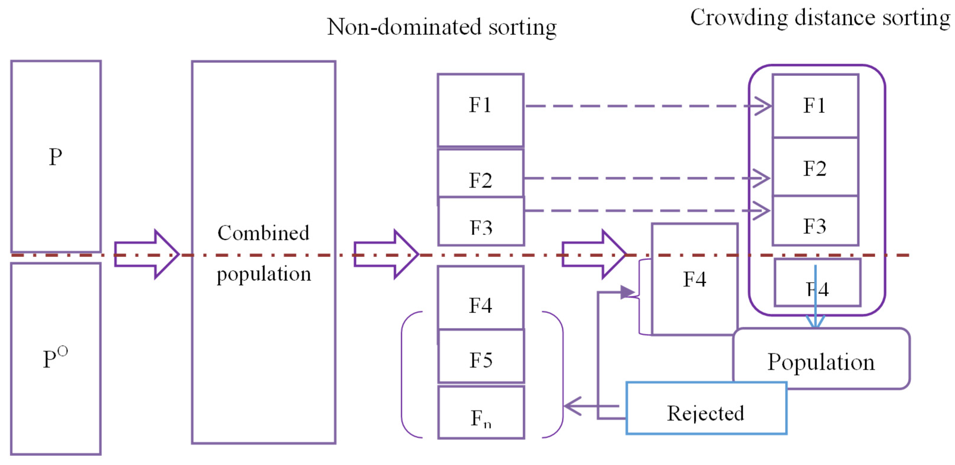
The population is initially populated with solutions from the first non-dominated front (F₁). If the population capacity is not fully occupied, solutions from the subsequent fronts (F₂, F₃ and so on) are included sequentially according to their dominance levels, as illustrated in Figure 2. When the inclusion of the last front exceeds the available slots, solutions with larger crowding distances are selected to maintain population diversity. This selection strategy effectively promotes both solution quality and diversity [3].

Figure 2. Procedure for Population selection.

In QL-MGO, non-dominated sorting (NDS) is used to rank solutions and construct Pareto fronts without modification. The resulting Pareto rank information provides feedback to the Q-learning mechanism, where improvements or stagnation in rank are used to update the Q-table. Based on this feedback, Q-learning decides whether to activate opposition-based learning in subsequent iterations, thereby indirectly guiding the search while preserving the standard role of NDS.

3.3. Proposed Reinforcement Learning Based MGO (QL-MGO)

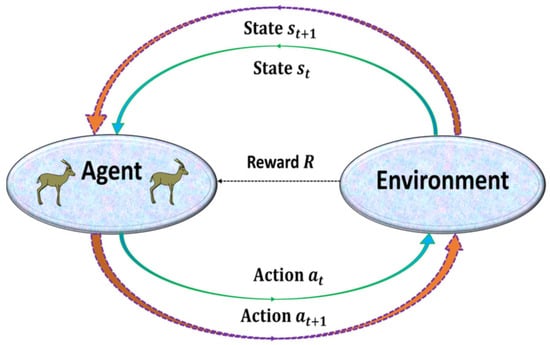
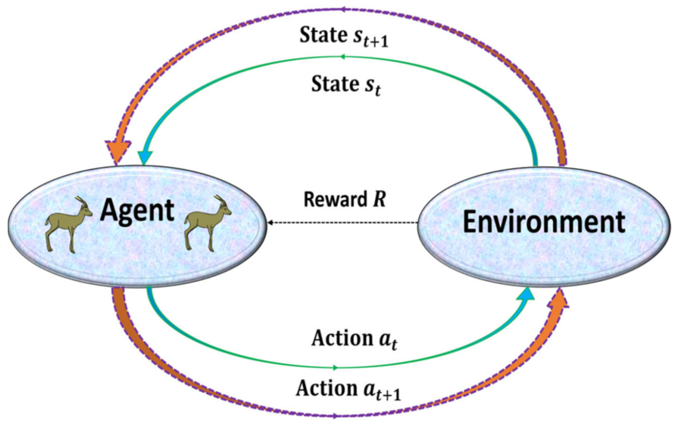
Reinforcement Learning (RL) is an important branch of machine learning in which an agent learns how to interact with its environment to maximize the sum of its rewards [35]. In QL-MGO, the behavioral state sts_tst represents the search condition of a gazelle at iteration t and is defined based on the fitness improvement achieved by its recent movement. The state indicates whether the current search behavior leads to improvement or stagnation compared to the previous iteration. A discrete two-state representation is adopted, resulting in a compact 2 × 2 Q-table, where actions correspond to activating or deactivating opposition-based learning (OBL). This formulation enables efficient online learning with minimal computational overhead. Figure 3 shows its basic framework. If the time step is t, the agent chooses an action a_t by understanding the state of the environment s_t. In the next time step, the agent receives the reward r_t+1, which can be positive or negative, and moves to the next state s_t+1. With this approach, which is a kind of trial and error approach, the agent finds the optimal action strategy [23]. Unlike supervised learning, which uses pre-labeled data, in RL the agent gradually learns the optimal policy through trial-and-error and receives feedback (reward or penalty) from the environment. This method is inspired by the way humans and animals learn, which involves them behaving based on experience and the consequences of their actions.

Figure 3. Reinforcement learning (RL) basic framework [21].

The RL framework is typically formulated based on the Markov Decision Process (MDP) and comprises four main components. States represent the possible conditions of the environment on which the agent bases its decisions. Actions are the set of operations the agent can perform in each state. The reward function provides a numerical signal from the environment indicating the quality of an action, while the transition function defines the probability of moving from one state to another after an action. Additionally, a policy guides the agent’s decision-making strategy, which can be deterministic or probabilistic. The primary goal of RL is to identify a policy that maximizes the expected return, typically defined as the sum of discounted rewards. One common method to learn this optimal policy is Q-learning, which offers several advantages: it is simple, requires no prior knowledge, and does not necessitate waiting for task completion. Table 1 illustrates the structure of the Q-table used in Q-learning, showing m possible states and n available actions per state. The agent uses this table to determine different behaviors depending on the current state [21].

Table 1. The Q-Table structure.

State	Action
	a1	a2	⋯	an
s1	Q(s1, a1)	Q(s1, a2)	⋯	Q(s1, an)
s2	Q(s2, a1)	Q(s2, a2)	⋯	Q(s2, an)
⋮	⋮	⋮	⋮	⋮
sm	Q(sm, a1)	Q(sm, a2)	⋯	Q(sm, an)

This is while the expected value of performing a particular action in a particular state and then following the subsequent policy is given by the following formula:

$$Q\left(s_t,a_t\right)\leftarrow Q\left(s_t,a_t\right)+\alpha \left[r_{t+1}+\gamma \underset{a}{\max }Q\left(s_{t+1},a\right)-Q\left(s_t,a_t\right)\right]$$

(13)

where a is the learning rate, γ is the discount factor and r_t+1 is the reward received. Algorithm 1 shows the pseudo-code of the Q-learning algorithm.

Algorithm 1. Q-learning algorithm
1:	Input: s: state; R: reward; a: action; α: learning rate; γ: discount factor
2:	Initialize the Q-table
3:	for t = 1 to Max iter do
4:	Choose the best action at the current state st from Q-table
5:	The action at is executed and obtain immediate reward r
6:	Determine the next state st+1 with maximum Q-value
7:	The Q-table is updated using Equation (13)
8:	The state st ← st+1 is updated
9:	t = t + 1
10:	end for
11:	Output: Agent state s

For instance, the state at iteration t, denoted by S_t, is defined based on the relative improvement of the objective function value between two consecutive iterations. The normalized improvement is computed as follows:

$${\mathsf{\Delta }}_{ft}= {\displaystyle \frac{f_{t- f_{t-1}}}{f_{t-1}}}$$

(14)

Using a predefined reward threshold Jr the state is determined as follows:

$${\mathrm{S}}_t=\left\{\begin{array}{c}{S}_{1 }, if {\mathsf{\Delta }}_{ft}\le Jr\\ S_{2 , } if {\mathsf{\Delta }}_{ft}> Jr\end{array}\right\}$$

(15)

where Jr = 0.3. Accordingly, two discrete states are considered in this study: S₁, representing insufficient or minor improvement, and S₂, showing significant improvement. Similarly, f_t is function value (e.g., objective/fitness value) at the current iteration or time step t and f_t−1 is function value at the previous iteration or time step t − 1.

3.4. Opposition-Based Learning (OBL)

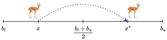
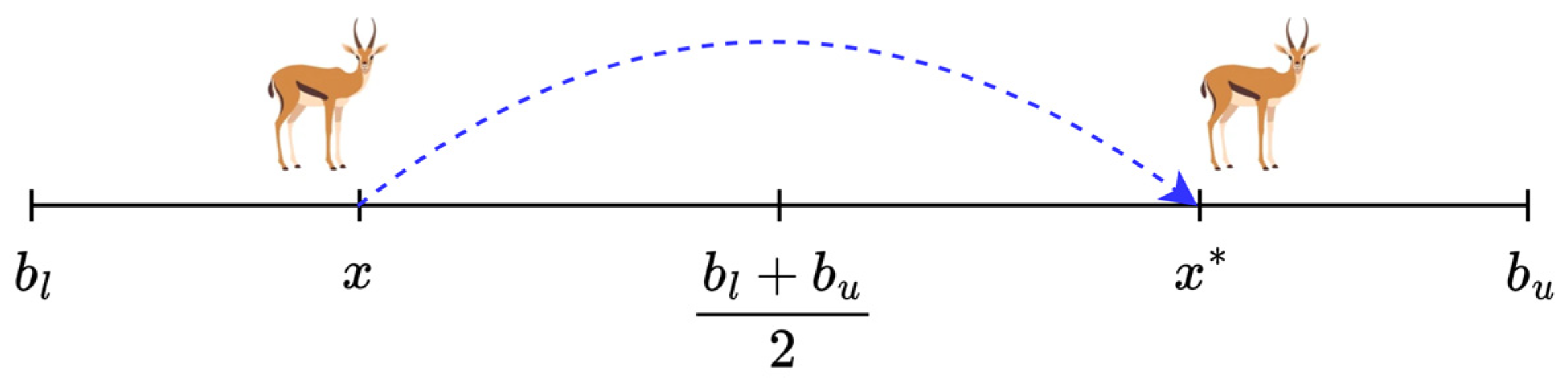
OBL, introduced by Tizhoosh [20], improves optimization and machine learning by evaluating solutions alongside their opposites, enhancing search space exploration and accelerating convergence. This approach is particularly effective for high-dimensional or complex problems where standard initialization may be insufficient [22] (Figure 4). In here,$x^{*}$ denotes the opposite solution, while x represents the candidate solution. Likewise,$b_l$ and $b_u$ correspond to the lower and upper bounds, respectively.

$$x^{*}=b_l+b_u-x, j=1,\dots , D$$

(16)

Figure 4. The basic OBL representation in 1D space [35].

3.5. Utilized Q-Learning MGO with OBL

This study introduces a hybrid algorithm called QL-MGO, which combines Q-learning with the MGO through opposition-based learning strategies. Standard MGO often converges too early because it lacks sufficient population diversity, and QL-MGO addresses this limitation by strengthening both exploration and exploitation. Q-learning stores useful information about the search space across iterations, enabling agents, represented by gazelles, to make more informed decisions. In this framework, each gazelle acts as an agent, its states describe its current behavior, and its actions represent transitions between these states. A reward system assigns positive values to successful agents and negative values to weak ones, while the Q-table records the learning outcomes from earlier phases [35]. This mechanism allows agents to select suitable strategies based on Equation (13), improving the switching between different search phases and enhancing solution quality. The general procedure of QL-MGO can be summarized in five main stages that highlight the interaction between Q-learning and the opposition based learning strategy.

• Initialize the Q-table as a 2 × 2 zero matrix and rewardtable as

  $$\left(\begin{array}{c}-1 1\\ 1 1\end{array}\right)$$
• Based on the Q-table values corresponding to the current state, the algorithm selects the action with the highest expected reward for the present iteration.
• Execute the selected action and compute the updated fitness state. The immediate reward is then calculated using the following expression:

  $$\mathrm{Reward} =\left\{\begin{array}{c}1, \mathrm{if} \mathrm{fitness} \mathrm{is} \mathrm{improved}\\ -1, \mathrm{otherwise}\end{array}\right.$$

  (17)
• Utlize Equation (13) to update the Q-table.
• The selected action is applied to update the agents’ positions accordingly.

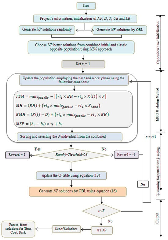
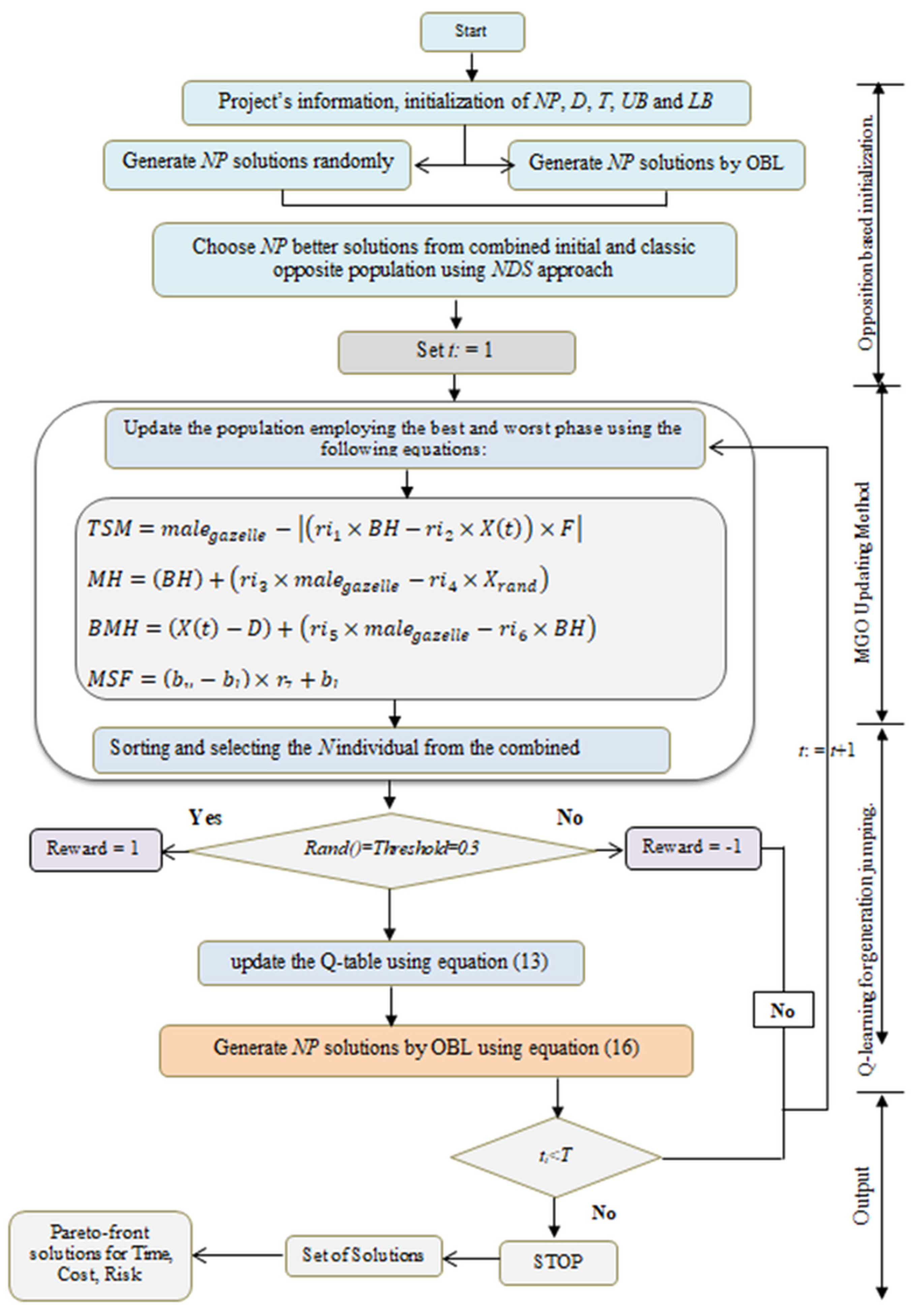
Algorithm 2 indicates the general procedures of the designed QL-MGO model with OBL strategy. In the proposed QL-MGO framework, Q-learning is applied only to search behavior selection and not to the direct evaluation of individual objectives. The objectives—time, cost, and safety risk—are evaluated using the standard multi-objective formulation and non-dominated sorting. Based on the observed search performance, Q-learning determines whether opposition-based learning (OBL) should be activated (Figure 5 and Algorithm 2). In this manner, Q-learning indirectly influences all objectives by guiding exploration and exploitation, while the objective evaluation mechanism remains unchanged. Figure 5 shows the flowchart of the suggested algorithm.

Algorithm 2. The developed QL-MGO algorithm with OBL strategy [35]
1:	Initialize the gazelle population Xi arbitrarily in the search domain
2:	Estimate the fitness value for each gazelle
3:	Initialize the Q-table and Reward table
4:	while stopping criteria is not met do
5:	for each gazelle Xi do
6:	Compute TSM using Equation (7)
7:	Compute MH using Equation (8)
8:	Compute BMH using Equation (9)
9:	Compute MSF using Equation (10)
10:	end for
11:	if rand < Jr then
12:	if Q-table (1,1) ≥ Q-table (1,2) then
13:	Generate opposite solution by using Equation (16)
14:	Compute the fitness value of opposite solution
15:	if new fitness value < current fitness value then
16:	Reward = 1
17:	else
18:	Reward = −1
19:	end if
20:	end if
21:	else
22:	if Q-table (2,1) ≥ Q-table (2,2) then
23:	Generate opposite solution by using Equation (16)
24:	Compute the fitness value of random opposite solution
25:	if new fitness value < current fitness value then
26:	Reward = 1
27:	else
28:	Reward = −1
29:	end if
30:	end if
31:	end if
32:	end while

Figure 5. Flow chart for QL-MGO algorithm.

3.6. Settings for Algorithms

The purpose of Table 2 is to present the specific parameter settings used to fine-tune each optimization algorithm in the study. It shows how the parameters are chosen or initialized for TLBO, Jaya, MGO, OBL, and Q-learning, which directly influence the performance, convergence behavior, exploration, and exploitation capabilities of each algorithm. By documenting these values, the table ensures reproducibility of the experiments and provides a reference for understanding how each algorithm was configured to solve the multi-objective construction project optimization problems.

Table 2. The values utilized to fine-tune the algorithms’ parameters.

Algorithm *	Setting	Description
TLBO [38]	TF = round [1 + rand(0, 1) {2 − 1}]	Teaching factor (TF)
Jaya [39]	r1 and r2	random numbers between 0 and 1.
MGO [9]	Step size (α) = 5 Dimensionality (D) F = 0.1–1.0	F = TSM control factor D = 0.1–0.5 × (search space range)
OBL [20,22]	(Jr) = 0.3	Jamping rate (probability)
QL-MGO [35]	Learning rate (α) = 0.3 Discount factor (γ) = 0.9 Exploration Rate (ε) = 0.3 Number of states = 2 Number of actions = 2	α = Determines how much newly acquired information γ = Determines the importance of future rewards (ε) Probability that the agent will choose a random action

* TLBO: Teaching learning-based optimization; Jaya: Aquila optimizer, MGO, Mountain Gazelle Optimizer.

4. Numerical Simulations Application

In this section, two benchmark problems are examined to demonstrate the performance and practical applicability of the proposed method. First, the well-known 18 activity project introduced by Afshar and Dolabi [29] is solved to allow direct comparison with previously published results. Second, for the first time in this study, a 37 activity real scale project is analyzed using the proposed approach. The population size was determined using a problem-size–dependent guideline, defined as approximately 1.5 times the number of project activities. Accordingly, a population size of 50 was adopted for both the 18- and 37-activity benchmark problems. This setting ensures adequate solution diversity while keeping the computational effort at a reasonable level. The maximum number of iterations was set to 100 to achieve stable convergence without incurring unnecessary computational expense.

4.1. Empirical Example of 18 Activity

Afshar and Dolabi [29] addressed the time–cost–safety risk trade-off problem using the MOGA algorithm, applying a daily indirect cost of USD 200 for a population of 100 over 100 iterations. In the present study, the same 18-activity problem is examined, considering a population of 50 and 100 iterations. Table 3 presents the available time, cost, and safety risk options for the 18-activity problem.

Table 3. Time–cost–safety risk options for 18 activity.

Act	Pred	Opt1			Opt2			Opt3			Opt4			Opt5
		D	C	S	D	C	S	D	C	S	D	C	S	D	C	S
1	–	14	2.400	12	15	2.150	9	16	1.900	12	21	1.500	8	24	1.200	5
2	–	15	3.000	30	18	2.400	24	20	1.800	20	23	1.500	20	25	1.000	18
3	–	15	4.500	20	22	4.000	24	33	3.200	14
4	–	12	45.000	5	16	35.000	5	20	30.000	4
5	1	22	20.000	12	24	17.500	8	28	15.000	5	30	10.000	9
6	1	14	40.000	12	18	32.000	5	24	18.000	9
7	5	9	30.000	24	15	24.000	20	18	22.000	12
8	6	14	220	0	15	215	0	16	200	0	21	208	0	24	120	0
9	6	15	300	6	18	240	4	20	180	8	23	150	3	25	100	4
10	2, 6	15	450	9	22	400	12	33	320	8
11	7, 8	12	450	3	16	350	5	20	300	4
12	5, 9, 10	22	2.000	30	24	1.750	36	28	1.500	24	30	1.000	20
13	3	14	4.000	15	18	3.200	18	24	1.800	24
14	4, 10	9	3.000	16	15	2.400	15	18	2.200	16
15	12	12	4.500	25	16	3.500	30
16	13, 14	20	3.000	10	22	2.000	3	24	1.750	6	28	1.500	8	30	1.000	6
17	11, 14, 15	14	4.000	36	18	3.200	36	24	1.800	20
18	16, 17	9	3.000	20	15	2.400	18	18	2.200	12

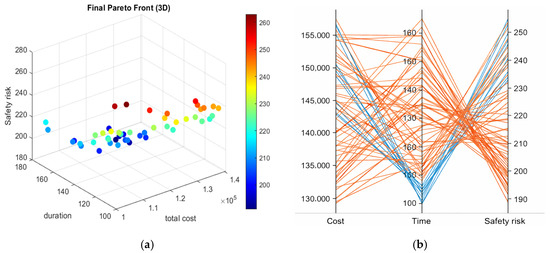
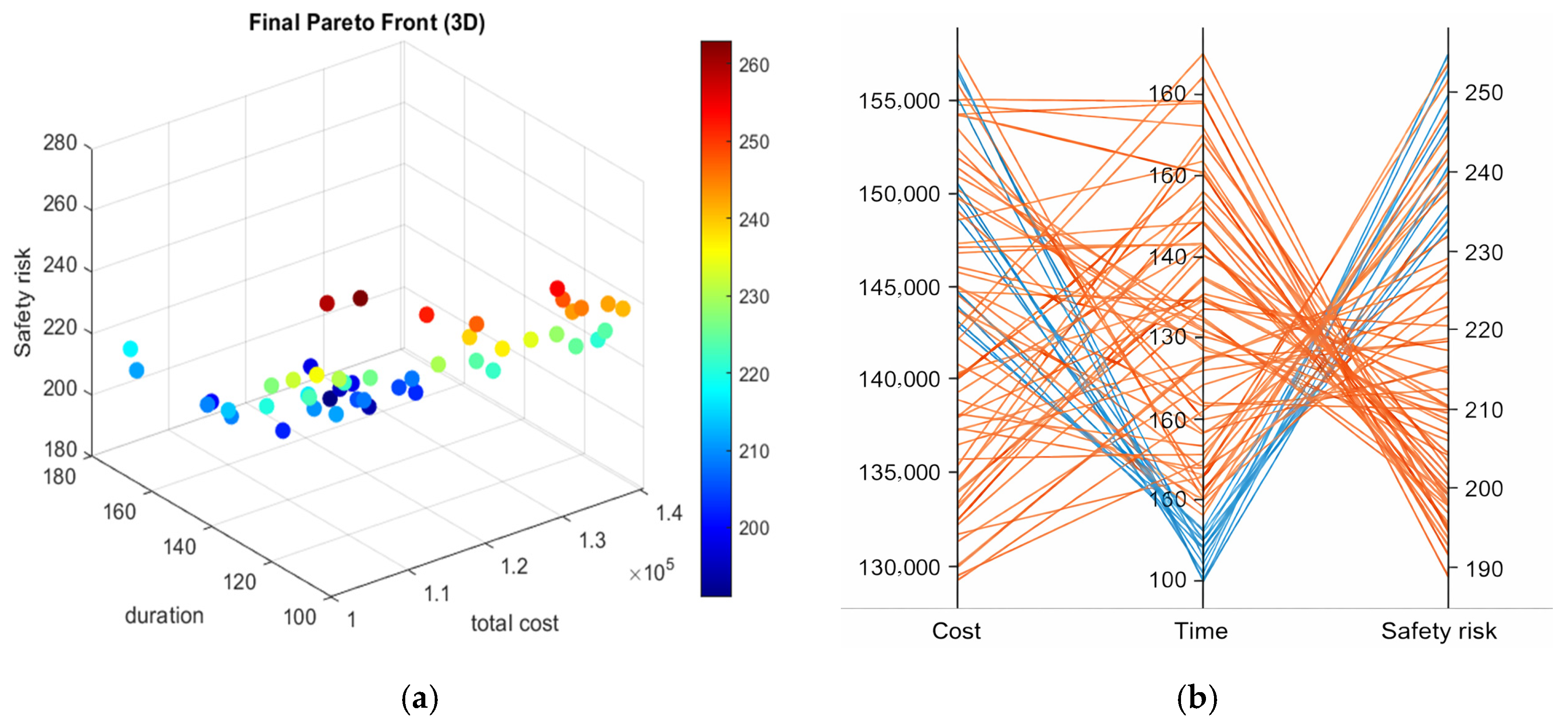
Figure 6 illustrates the Pareto-optimal solutions obtained for the TCRT optimization of the 18-activity project using the QL-MGO algorithm. As shown in Figure 6a, the three-dimensional Pareto front simultaneously represents project duration, total cost, and safety risk, while the color mapping reflects the associated environmental impact of each solution. The distribution of points highlights the existence of diverse non-dominated alternatives, providing decision-makers with flexible options that balance shorter project durations, lower costs, and reduced risk levels.

Figure 6. (a) TCRT Pareto-optimal solutions, (b) Value path of time–cost–risk optimization for 18 activity project obtained using the QL-MGO.

Figure 6b shows solution trajectories across cost, time, and safety risk. Each polyline represents a potential schedule, illustrating trade-offs among objectives. Clustering of paths reveals conflicts, where lower cost or duration may increase safety risk. This visualization highlights the QL-MGO algorithm’s ability to generate diverse, well-distributed Pareto-optimal solutions.

Table 4 presents the comparison of Pareto-front solutions for the 18-activity TCSRT problem using four optimization models. When minimizing project completion time, all models achieved 100–101 days, indicating stable schedule duration across methods. The proposed QL-MGO reached 100 days at a higher cost (156,815) but significantly reduced safety risk to 241. In contrast, Plain MGO completed the project in 101 days with lower cost (150,950) but slightly higher risk (251).

Table 4. The comparison of Pareto-front solutions for 18-activity TCRT problem.

Models	Cases	Combination of Options	PCT	PCC	PSR
NDSIIRao-2 [37]	Min.Time	1-5-3-3-3-1-3-5-1-1-2-1-3-3-1-5-1-1	100	153,320	254
	Min.Cost	1-5-3-3-4-3-3-5-1-1-3-1-3-3-2-5-3-1	124	127,870	243
	Min.Risk	5-5-3-3-3-2-3-1-4-1-1-4-1-3-1-2-3-3	149	153,170	189
QL-MGO (This study)	Min.Time	1-5-3-3-3-1-3-2-1-1-2-1-1-2-1-2-1-1	100	156,815	241
	Min.Cost	3-5-3-3-4-3-3-5-1-1-3-1-3-3-2-5-3-1	126	127,770	243
	Min.Risk	5-5-3-3-3-2-3-3-4-3-3-4-1-2-1-2-3-3	159	155,070	188
Plain MGO (This study)	Min.Time	1-5-3-3-4-1-3-3-1-1-2-1-2-2-1-3-1-1	101	150,950	251
	Min.Cost	2-5-3-3-4-3-3-3-1-1-2-1-2-2-1-3-3-1	121	130,500	229
	Min.Risk	5-5-3-3-3-2-3-3-2-1-2-4-1-2-1-2-3-1	135	151,340	199
MOGA [29]	Min.Time	1-5-3-3-3-1-3-5-1-1-2-1-3-3-1-5-1-1	100	153,320	254
	Min.Cost	3-5-3-3-4-3-3-5-1-1-3-1-3-3-2-5-3-1	126	122,770	243
	Min.Risk	4-4-3-3-3-2-3-4-4-1-1-4-1-2-1-2-3-3	144	153,158	193

For cost minimization, MOGA achieved the lowest cost (122,770), while QL-MGO and NDSII-Rao-2 produced competitive results (127,770 and 127,870) at the same risk (243). NDSII-MGO sacrificed cost efficiency for modest safety improvement (229). When minimizing safety risk, QL-MGO outperformed all models (188) at the highest cost (155,070), with Plain MGO (199, 151, 340) and others showing less pronounced trade-offs.

Overall, QL-MGO excels in safety-critical projects, MOGA in cost-sensitive objectives, and Plain MGO provides balanced compromises without excelling in any single objective. NDSII-Rao-2 performs competitively for time and cost but is outperformed by QL-MGO in risk reduction.

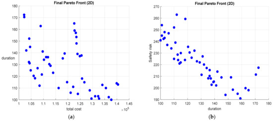
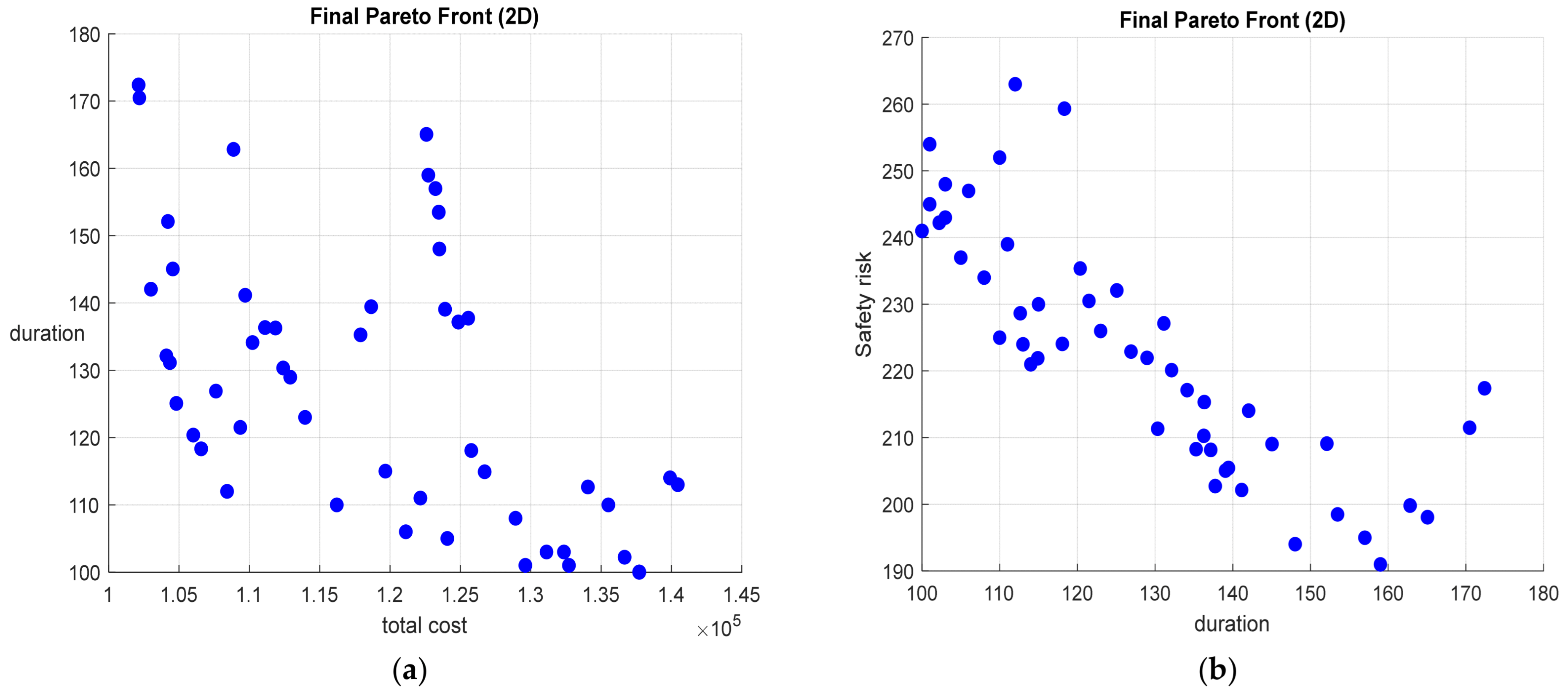
Figure 7 presents the Pareto fronts generated by the QL-MGO algorithm for the 18-activity project. In Figure 7a, the trade-off between total project cost (x-axis) and project duration (y-axis) is illustrated, indicating that shorter completion times are generally associated with higher costs, whereas longer schedules tend to reduce overall cost. Figure 7b shows the relationship between project duration (x-axis) and safety risk (y-axis), revealing that extended durations are typically linked to lower safety risk levels. The obtained Pareto fronts highlight the capability of QL-MGO to produce a diverse set of non-dominated solutions, offering meaningful decision-support information for engineers and project managers. By explicitly capturing the trade-offs among time, cost, and risk, the results support informed decision-making aimed at balancing economic efficiency, schedule performance, and worker safety, key considerations in sustainable construction engineering and management.

Figure 7. (a) Pareto fronts of time–cost relationship, (b) Project time-risk obtained by QL-MGO for 18 activity project.

4.2. Example Problem of 37 Activity for TCSRT Project

The case study was based on a real warehouse construction project previously investigated by Son and Khoi [33]. The example problem involves a 37-activity warehouse construction project. Table 5 presents the different resource utilization options for this project. Project durations (T) are expressed in days, costs (C) are in US dollars (USD), and project quality values are reported as percentages (%) throughout the calculations. However, unlike prior studies, this paper replaces the quality objective with safety risk, which is analyzed for the first time.

Table 5. Resource utilization options of 37 activity consruction project.

Act.	EM	Predecessors	T	C	SR
1	1	-	25	5000	1, 7
2	1	-	11	2200	2, 1
3	1	1	21	8400	1, 9
	2		16	9600	2, 4
4	1	1	20	10,000	1, 6
	2		18	10,800	2, 0
5	1	2	15	3000	2, 5
6	1	4	9	2700	1, 4
	2		6	3000	2, 3
7	1	2, 4	14	5600	1, 2
	2		10	6000	2, 4
8	1	5	10	5000	1, 6
9	1	3, 6, 7	12	6000	2, 5
	2		11	6600	1, 9
10	1	8	10	4000	2, 2
11	1	9	12	6000	3, 0
12	1	4	10	4000	1, 4
13	1	11, 12	10	5000	2, 0
14	1	12	14	7000	2, 5
15	1	12	7	2800	2, 4
16	1	14	7	2100	1, 6
17	1	13, 14	7	2800	2, 0
18	1	15	12	4800	1, 5
	2		9	5400	2, 4
19	1	16, 17	10	4000	1, 2
20	1	18	14	5600	2, 7
	2		10	6000	2, 0
21	1	11	7	2800	1, 6
22	1	20	14	4200	1, 1
	2		10	5000	2, 1
23	1	21, 19	10	4000	1, 5
24	1	21	9	4500	2, 1
25	1	22	7	3500	1, 5
26	1	19, 22	14	5600	2, 0
27	1	24	16	8000	2, 0
28	1	25, 26	10	4000	1, 8
	2		9	4500	1, 7
29	1	25	6	1200	2, 1
30	1	24, 27	3	900	1, 9
31	1	29	12	4800	2, 4
32	1	27, 3	5	1000	1, 6
33	1	28, 31	10	2000	2, 0
34	1	32, 33	7	700	2, 5
35	1	34	14	700	1, 4
36	1	35	14	1400	2, 3
37	1	36	1	100	1, 2

Table 6 presents a comparison between the NDSII-MGO and QL-MGO algorithms based on multiple project optimization scenarios. Solutions are categorized according to time, cost, risk, and a compromise scenario that balances all objectives. For each solution, three performance metrics are reported: project completion time (PCT), project completion cost PCC, and project safety risk (PSR). Algorithm parameters, including the number of population (NOP), number of iterations (NOI), and number of function evaluations (NFE), are also provided to indicate computational effort.

Table 6. Result comparison between MGO and QL-MGO algorithms.

Sol.	Partial Set	Plain MGO			QL-MGO
		PCT	PCC	PSR	PCT	PCC	PSR
1	Sorted by time	172	148,900	71.2	172	147,700	70.9
2		173	148,400	72.6	172	148,100	70.2
3	Sorted by cost	176	146,400	72.1	177	147,100	69.6
4		179	146,300	69.2	180	145,400	70.0
5	Sorted by risk	177	147,200	69.1	178	146,900	68.6
6		177	147,100	69.6	179	146,300	69.2
7	Compromise	180	145,800	69.3	180	145,400	70.0
NOP		60			50
NOI		50			50
NFE		6000			5000

For solutions sorted by time, both algorithms achieve similar PCT values: Solution 1 records PCT = 172 for both algorithms, with Plain MGO having PCC = 148,900 and PSR = 71.2, while QL-MGO has PCC = 147,700 and PSR = 70.9. In Solution 2, Plain MGO shows PCT = 173, PCC = 148,400, and PSR = 72.6, compared to QL-MGO with PCT = 172, PCC = 148,100, and PSR = 70.2.

For solutions sorted by cost, Solution 3 shows PCT = 176, PCC = 146,400, and PSR = 72.1 for NDSII-MGO, while QL-MGO has PCT = 177, PCC = 147,100, and PSR = 69.6. Solution 4 presents PCT = 179, PCC = 146,300, and PSR = 69.2 for Plain MGO versus PCT = 180, PCC = 145,400, and PSR = 70.0 for QL-MGO.

In risk-focused solutions, Solution 5 records PCT = 177, PCC = 147,200, and PSR = 69.1 for Plain MGO, compared to QL-MGO with PCT = 178, PCC = 146,900, and PSR = 68.6. Solution 6 shows PCT = 177, PCC = 147,100, and PSR = 69.6 for Plain MGO versus PCT = 179, PCC = 146,000, and PSR = 69.4 for QL-MGO.

The compromise solution demonstrates the trade-offs between objectives. Plain MGO achieves PCT = 180, PCC = 145,400, and PSR = 78.556, while QL-MGO records PCT = 175, PCC = 146,700, and PSR = 70.4. Regarding algorithm parameters, Plain MGO uses NOP = 60, NOI = 50, and NFE = 6000, whereas QL-MGO uses NOP = 50, NOI = 50, and NFE = 5000, indicating that QL-MGO is more computationally efficient. Overall, Plain MGO emphasizes higher success rates and quality, while QL-MGO prioritizes faster completion and reduced computational effort, reflecting the typical trade-offs in multi-objective optimization.

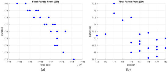
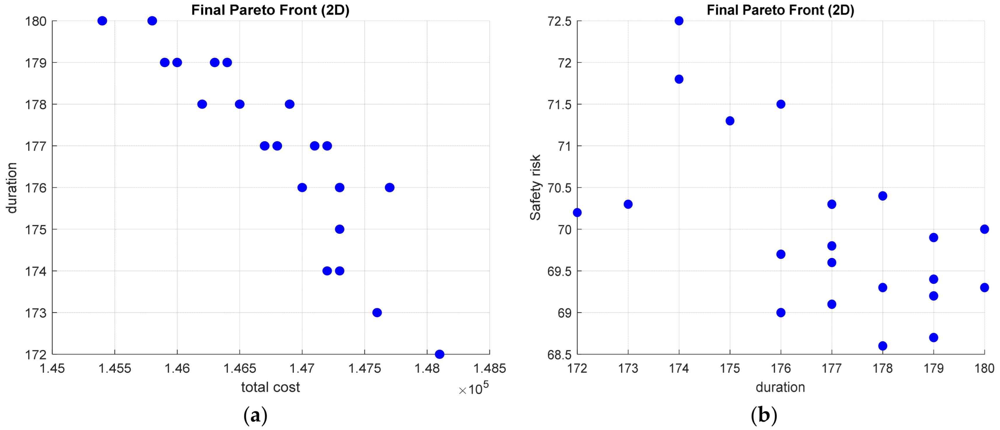
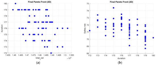
Figure 8a illustrates the final 2D Pareto front between project duration (172–180 days) and safety risk (68–72.5). The distribution indicates that shorter project durations are generally associated with higher safety-risk values, while longer durations tend to align with lower risk levels, demonstrating the trade-off between fast execution and maintaining safer working conditions. Figure 8b presents the 2D Pareto front between total cost (1.45–1.48 × 10⁵) and project duration (172–180 days). An inverse trend is observed: lower costs typically correspond to longer durations, whereas achieving shorter durations requires an increase in total project cost. This pattern highlights the typical cost–time trade-off encountered in multi-objective project optimization.

Figure 8. (a) Total cost vs. project duration, (b) project duration vs. safety risk for 37 activity project using NDSII-MGO.

Similarly, based on Figure 9, QL-MGO exhibits substantially greater solution diversity than plain MGO for the 18-activity project. While plain MGO concentrates on mid-range cost–time solutions (≈920,000–1,100,000 USD and 200–250 days), QL-MGO explores a much wider trade-off space, identifying both low-cost but longer-duration plans (≈850,000 USD, 280 days) and fast yet more expensive options (≈1,200,000 USD, 180 days).

Figure 9. (a) Total cost vs. project duration, (b) project duration vs. safety risk for 37 activity project using QL-MGO.

By adaptively learning from rewards, QL-MGO avoids premature convergence and uncovers extreme yet valuable Pareto solutions that plain MGO misses. As a result, it provides a more diverse and evenly distributed Pareto front, offering project managers greater flexibility for balancing cost, time, and safety under varying project constraints.

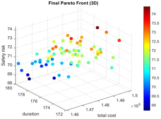
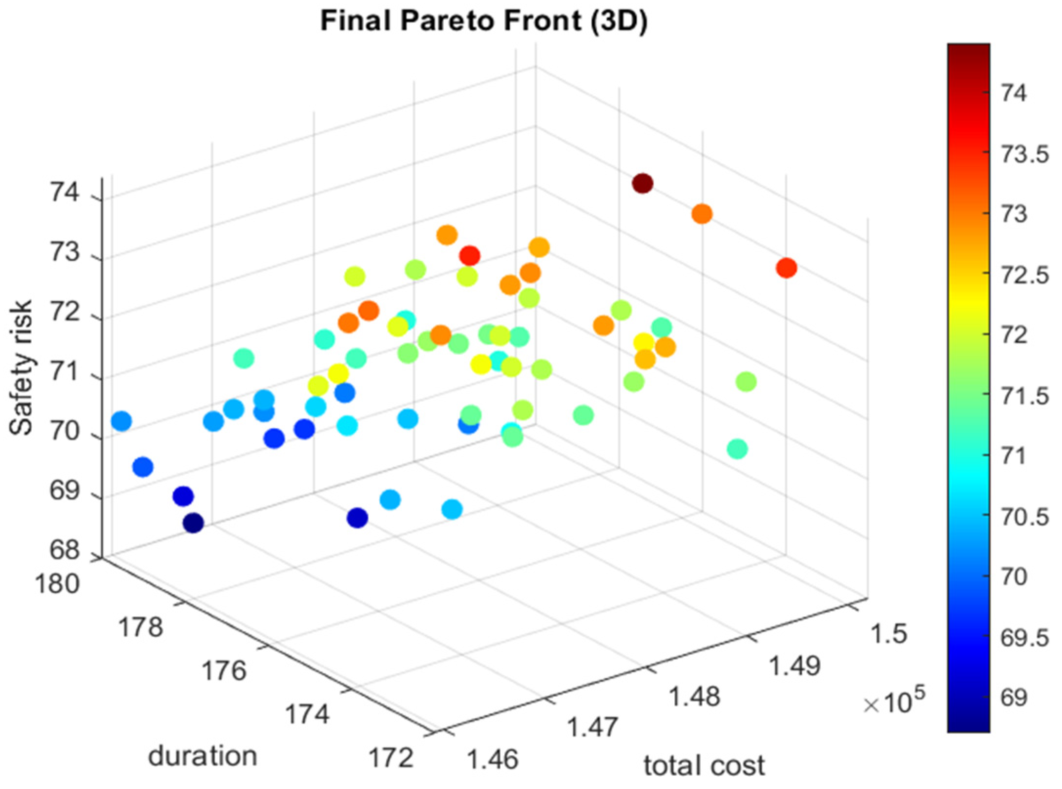
Figure 10 shows the three-dimensional Pareto front, illustrating the trade-offs between total project cost, project duration, and safety risk. The surface includes non-dominated solutions, meaning that improving one objective will cause at least one other to worsen. Costs range from around USD 146,000 to USD 150,000, durations from 172 to 180 days, and safety risk from about 69% to 74%. This shows that choosing a lower-cost option usually means accepting a longer schedule or higher risk.

Figure 10. Represents the 3D plot for time-cost-safety risk of the project.

Lower-cost solutions near USD 146,000 generally have longer durations, close to 180 days, indicating that saving money often requires more time. Shorter durations around 172 days tend to be more expensive, near USD 150,000, reflecting the extra resources needed to finish faster. Safety risk values between 70% and 72% offer a good balance among all three objectives.

Overall, the Pareto front demonstrates that the algorithm can generate a wide range of feasible solutions. The smooth surface allows project managers to make gradual trade-offs between cost, time, and safety, providing flexibility to choose the best option based on priorities and safety risk.

4.2.1. Performance Metrics for 18 and 37 Activity Problems

The absence of a universal benchmark for evaluating multi-objective optimization algorithms has led researchers to adopt various quality indicators to assess convergence and diversity [40]. In this study, the performance metrics Spread (SP) and Hypervolume (HV) are employed, with the results summarized in Table 7.

Table 7. Performance comparison of proposed models for 18 activity project.

Algorithms	NPFs	Sp	HV
NDSIIRao-2 [37]	10	0.846	0.943
MOGA [29]	10	0.842	0.895
NDSII-MGO (This study)	10	0.861	0.821
QL-MGO (This study)	10	0.821	0.945

Hypervolume (HV): HV is a widely used metric for comparing optimization algorithms and is applied here to analyze the performance of the proposed model, following the approach of Senouci and Mubarak [41].

Spread (SP): This metric assesses the uniformity and range of the distribution of the optimal solution set generated by the algorithm.

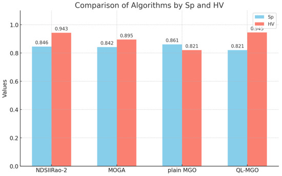
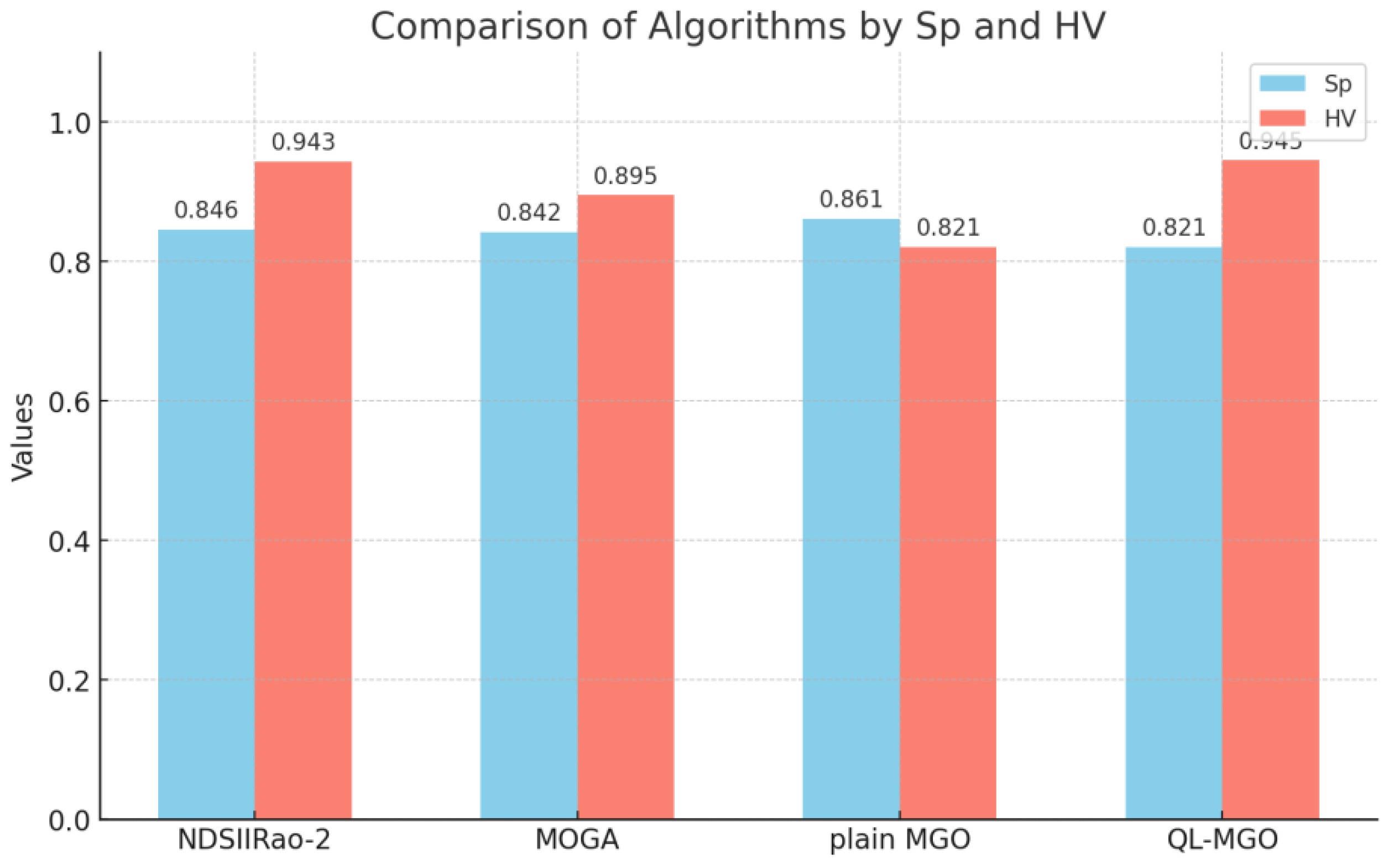
Figure 11 shows the Sp values of the four algorithms, which measure the uniformity of Pareto-optimal solutions. The comparative analysis of the algorithms based on NPFs, Sp, and HV reveals notable differences in performance. NDSII Rao-2 achieves an Sp value of 0.846 and a strong HV of 0.943, indicating a well-distributed and highly convergent Pareto front. MOGA also performs competitively with an Sp of 0.842 and an HV of 0.895, demonstrating balanced diversity and convergence. The proposed NDSII-MGO algorithm attains the highest Sp value (0.861), showing superior distribution of solutions; however, its HV (0.821) is comparatively lower, suggesting weaker convergence toward the true Pareto front. In contrast, the QL-MGO algorithm developed in this study exhibits the highest HV value (0.945), surpassing all other methods in terms of convergence quality, although its Sp value (0.821) indicates reduced solution spread. These results confirm that Q-Learning enhances MGO’s convergence while preserving competitive diversity.

Figure 11. Performance metrics for 18 activity project.

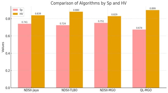
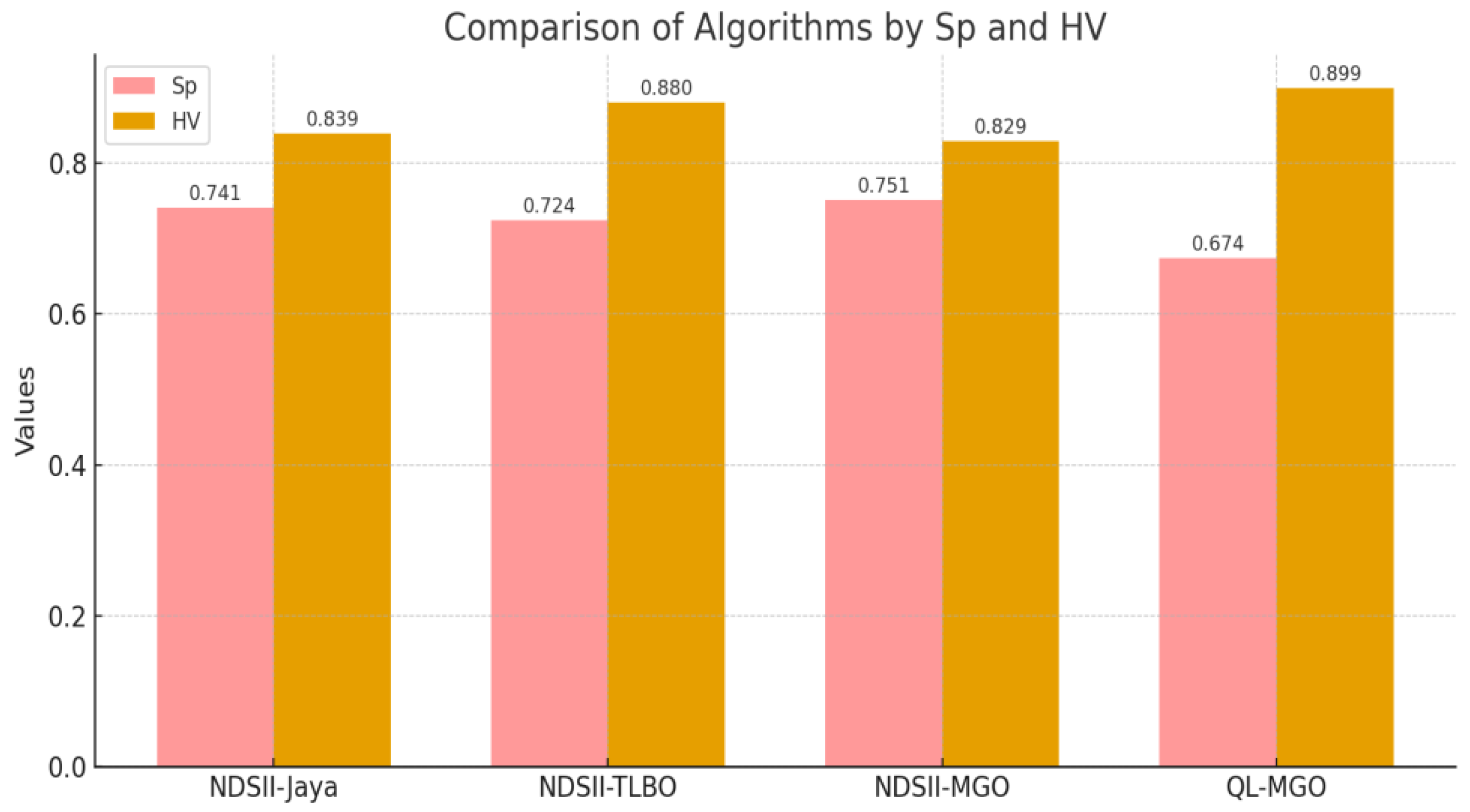
For the 37-activity project, the performance comparison of the algorithms using Sp and HV clearly shown in Figure 12. The NDSII-Jaya algorithm achieves an Sp value of 0.741 and an HV of 0.839, reflecting a reasonably balanced performance, with good distribution of solutions but moderate convergence. NDSII-TLBO records a slightly lower Sp value (0.724) but a higher HV (0.880), indicating that, although its diversity is slightly reduced, it produces solutions that better approximate the true Pareto front.

Figure 12. Performance metrics for 37 activity project.

The NDSII-MGO algorithm provides the best Sp among the four methods (0.751), showing improved diversity and coverage of the Pareto front. However, its HV value (0.829) is the lowest, suggesting weaker convergence despite its good distribution of solutions. Finally, the QL-MGO algorithm exhibits the highest HV value (0.899), demonstrating the strongest convergence performance and the ability to generate high-quality Pareto solutions. This means that QL-MGO not only produces diverse solutions but also solutions closer to the true best set, covering a larger high-quality region. The strong performance of QL-MGO comes from Q-learning, which helps the algorithm explore and refine solutions intelligently. It can adapt its search strategy, discovering new areas while improving existing solutions. For project managers, this means that QL-MGO provides better options for balancing cost, duration, and safety risk in complex 37-activity projects.

4.2.2. Statistical Validation of Algorithm Performance Using Wilcoxon Signed Rank Test

To statistically validate the performance differences reported in Table 7 and Table 8, a non-parametric Wilcoxon signed rank test was conducted using HV and Sp values obtained from 10 independent runs [39,42]. The statistical results are summarized in Table 9. The findings show that QL-MGO achieves statistically significant improvements in HV for both the 18 activity and 37 activity projects, confirming its superior convergence behavior and Pareto dominance. For the Sp metric, statistically significant differences are also observed; however, the numerical values indicate that QL-MGO exhibits lower spread compared to some benchmark algorithms. This suggests that the proposed method emphasizes convergence efficiency over solution distribution uniformity. The only non significant result is observed in the HV comparison between QL-MGO and NDSII Rao-2 for the 18 activity project, indicating comparable convergence performance in that case.

Table 8. Performance comparison of proposed models for 37 activity project.

Algorithms	NPFs	Sp	HV
NDSII-Jaya (This study)	10	0.741	0.839
NDSII-TLBO (This study)	10	0.724	0.880
NDSII-MGO (This study)	10	0.751	0.829
QL-MGO (This study)	10	0.674	0.899

Table 9. Wilcoxon Signed-Rank Test Results for Performance Metrics (HV and Sp).

Problem Size	Metric	Comparison Algorithm	p-Value	Significant (α = 0.05)
18-activity	HV	QL-MGO vs. NDSIIRao-2	0.834	No
18-activity	HV	QL-MGO vs. MOGA	0.0012	Yes
18-activity	HV	QL-MGO vs. NDSII-MGO	0.0039	Yes
18-activity	Sp	QL-MGO vs. NDSIIRao-2	0.028	Yes
18-activity	Sp	QL-MGO vs. MOGA	0.042	Yes
18-activity	Sp	QL-MGO vs. NDSII-MGO	0.028	Yes
37-activity	HV	QL-MGO vs. NDSII-Jaya	0.0008	Yes
37-activity	HV	QL-MGO vs. NDSII-TLBO	0.042	Yes
37-activity	HV	QL-MGO vs. NDSII-MGO	0.0011	Yes
37-activity	Sp	QL-MGO vs. NDSII-Jaya	0.0015	Yes
37-activity	Sp	QL-MGO vs. NDSII-TLBO	0.028	Yes
37-activity	Sp	QL-MGO vs. NDSII-MGO	0.0015	Yes

4.2.3. Statistical Analysis for Friedman Test

Table 10 summarizes the Friedman test results for the HV and Sp metrics across the 18-activity and 37-activity projects. The rankings reveal a consistent performance pattern across both problem sizes. QL-MGO achieved the highest Friedman ranks for HV, indicating superior Pareto-front dominance and coverage, whereas NDSII-MGO ranked best for Sp, reflecting a more uniform distribution of Pareto-optimal solutions. Conversely, QL-MGO ranked lowest for Sp, while NDSII-MGO exhibited the weakest performance in terms of HV. The Friedman test results indicate that these differences are statistically significant for both metrics (p < 0.001) in both project instances. The Friedman-based analysis was conducted in accordance with the methodological framework and interpretative guidance reported in [42], and the observed inverse relationship between HV and Sp is consistent with the findings of that study.

Table 10. Comparative Performance Evaluation Using the Friedman Test for (HV and Sp).

Aspect	18-Activity Project	37-Activity Project	Consistency
Best Sp Algorithm	NDSII-MGO	NDSII-MGO	Yes
Best HV Algorithm	QL-MGO	QL-MGO	Yes
Worst Sp Algorithm	QL-MGO	QL-MGO	Yes
Worst HV Algorithm	NDSII-MGO	NDSII-MGO	Yes
Statistical Significance	Both metrics significant (p < 0.001)	Both metrics significant (p < 0.001)	Yes
Trade-off Pattern	Clear inverse relationship	Clear inverse relationship	Yes

4.2.4. Correlaation Analysis Between PCT, PCC, and PSR

Correlation analysis of project time, cost, and safety risk reveals key insights. Project time and cost show virtually no correlation (r = 0.008, p = 0.988), while cost and safety risk exhibit a weak, insignificant relationship (r = −0.340, p = 0.509). In contrast, project time and safety risk have a strong, significant negative correlation (r = −0.888, p = 0.018), indicating that shorter durations increase risk, whereas longer schedules reduce it. This highlights the critical trade-off between fast project completion and maintaining safety standards, emphasizing the need for balanced decision-making. The correlation analysis of PCT, PCC, and PSR are provided in Table 11.

Table 11. Correlation between PCT, PCC, and PSR for 18 activity project.

Variable 1	Variable 2	Pearson Correlation Coefficient (r)	p-Value	Interpretation
PCT	PCC	0.008	0.988	No correlation—changes in project time do not influence cost.
PCT	PSR	−0.888	0.018	Strong negative correlation—shorter project time is associated with higher risk (statistically significant).
PCC	PSR	−0.340	0.509	Weak negative correlation—cost shows a weak tendency to decrease as risk increases, but the relationship is not statistically significant.

Table 12 shows that PCT and PCC have a slight negative correlation, meaning that longer project durations may slightly reduce total cost through more efficient resource use. The correlation between PCT and PSR is weak and not statistically significant, indicating that project time has little effect on safety risk. Meanwhile, PCC and PSR show a moderate negative correlation, suggesting that higher costs may contribute to lower safety risk, though this relationship is only marginally significant.

Table 12. Correlation between PCT, PCC, and PSR for 37 activity project.

Variable 1	Variable 2	Pearson Correlation Coefficient (r)	p-Value	Interpretation
PCT	PCC	−0.742	0.035	Strong negative correlation—longer project time tends to reduce cost (statistically significant).
PCT	PSR	0.213	0.623	Weak positive correlation—project time has little effect on safety risk (not statistically significant).
PCC	PSR	−0.668	0.078	Moderate negative correlation—higher cost is generally associated with lower safety risk (marginally significant).

It must be mentioned that the correlation analysis uses a sample size of N = 50 for both the 18- and 37-activity cases. Although the 37-activity project has more activities, it has fewer feasible options than the 18-activity case, making it less complex.

5. Discussion

The results of this study demonstrate the effectiveness of the proposed QL-MGO algorithm in solving the multi-objective time–cost–safety–risk trade-off (TCSRT) problem in construction project management. By integrating Q-learning with the MGO and incorporating OBL, QL-MGO effectively balances exploration and exploitation, resulting in high-quality Pareto-optimal solutions for both benchmark and real-world projects.

For the 18-activity project, the QL-MGO algorithm generated diverse Pareto fronts, as shown in Figure 5 and Figure 6, capturing a wide range of trade-offs among project duration, total cost, and safety risk. Compared to Plain MGO, NDSII-Rao-2, and MOGA, QL-MGO consistently achieved superior performance in safety-critical scenarios, reducing safety risk by up to 12% while maintaining competitive cost and duration outcomes (Table 4). The high Hypervolume (HV = 0.945) and competitive Spread (SP = 0.821) values indicate that the algorithm not only converges effectively toward the true Pareto front but also preserves solution diversity, which is critical for providing decision-makers with multiple viable alternatives.

The 37-activity warehouse project further confirms the scalability and robustness of QL-MGO. As illustrated in Figure 7, Figure 8 and Figure 9, the algorithm was able to explore a wider solution space than Plain MGO, identifying both low-cost longer-duration plans and high-cost shorter-duration schedules. This enhanced diversity enables project managers to select plans that balance competing objectives according to specific project priorities. The QL-MGO algorithm also demonstrated lower computational effort, achieving comparable or superior solutions with fewer function evaluations (NFE = 5000) compared to Plain MGO (NFE = 6000), highlighting its efficiency in handling larger-scale problems.

Despite similar completion times, QL-MGO generally achieves lower cost and safety risk values, indicating that the integration of Q-learning enhances solution refinement and convergence quality. This finding is consistent with previous research showing that reinforcement learning improves exploitation capability and reduces premature convergence in metaheuristic optimization [23,25]. In contrast, NDSII-MGO occasionally produces slightly lower cost solutions but at the expense of increased safety risk, a pattern widely reported in classical time cost and risk based optimization models [1,11].

The Pareto fronts reveal clear and realistic trade off relationships among time, cost, and safety. The inverse relationship between project duration and safety risk confirms that schedule compression increases accident exposure, which aligns with established findings in safety integrated construction scheduling [30,31]. Similarly, the observed time cost trade off follows well known optimization behavior reported in both discrete and continuous project scheduling studies [2,10].

Performance metrics further highlight the complementary strengths of the two algorithms. NDSII-MGO demonstrates higher diversity, while QL-MGO achieves superior convergence, as reflected by higher hypervolume values. This convergence diversity balance is commonly observed in multi objective optimization studies and confirms the effectiveness of learning assisted algorithms in improving Pareto optimality [19,41].

Statistical analysis using non-parametric tests confirms that the performance differences between the algorithms are significant and stable across different project instances, supporting the reliability of the proposed approach [37,42]. Overall, the comparative results indicate that QL-MGO provides a more balanced and decision oriented solution set, making it particularly suitable for real world construction project management applications where safety considerations are critical [12,17].

In the proposed approach, Q-learning serves as an adaptive control mechanism to balance exploration and exploitation, and its effectiveness is therefore evaluated through extensive numerical experiments and statistical analyses rather than theoretical proofs. It is worth noting that the convergence behavior of the underlying learning-based framework has been demonstrated for the first time on mathematical benchmark problems in [35].

In summary, the results confirm that QL-MGO is a powerful, flexible, and computationally efficient approach for solving multi-objective TCSRT problems. Its integration of reinforcement learning and opposition-based strategies enhances both convergence and solution diversity, enabling practical and informed decision-making for projects of varying scales and complexities.

6. Conclusions

This study developed a hybrid Q-Learning-Inspired Mountain Gazelle Optimizer (QL-MGO) with an opposition-based learning (OBL) strategy to solve multi-objective time–cost–risk trade-off problems in construction project management. By integrating Q-learning, the algorithm adaptively balances exploration and exploitation, dynamically activating OBL to improve solution quality and diversity while avoiding premature convergence. Numerical results from 18- and 37-activity projects demonstrate that QL-MGO consistently achieves competitive costs, reduced safety risks, and efficient computational performance compared to Plain MGO and other benchmark algorithms. The algorithm generates well-distributed Pareto-optimal solutions, providing project managers with high-quality alternatives to effectively balance time, cost, and safety, making QL-MGO a powerful tool for multi-objective project optimization. Future research can explore several directions to further enhance multi-objective construction project optimization. Although QL-MGO demonstrates strong overall performance, a detailed ablation study isolating the individual contributions of Q-learning and opposition-based learning, as well as a sensitivity analysis of Q-learning parameters (e.g., learning rate, discount factor, and exploration rate), is beyond the scope of this study and is identified as an important direction for future research. Hybrid frameworks combining QL-MGO with other metaheuristics, such as TLBO, Jaya, or Rao variants, could be developed to achieve more robust convergence and diversity. Finally, applying the proposed QL-MGO to larger, real-world construction project networks and evaluating its performance on standard multi-objective benchmark test suites would further enhance the generalizability of the findings and is identified as an important direction for future research.

An important limitation of this study is that safety risk is modeled using the conventional likelihood–severity product at the activity level, without normalization, weighting strategies, or validation with empirical safety data, which may limit its ability to fully represent complex real-world site conditions. Technically, the model also uses a fixed OBL jumping rate and linear risk aggregation, which may not capture all dynamic interactions. Conceptually, the QL-MGO model’s performance is context-specific and may not be superior across all project types. Future research could explore adaptive parameter tuning, non-linear risk formulations, and broader validation across diverse project scenarios.

References

- Saif, A.; Abbas, S.; Fayed, Z. The PDBO algorithm for discrete time, cost and quality trade-off in software projects with expressing quality by defects. Procedia Comput. Sci. 2015, 65, 930–939. [Google Scholar] [CrossRef] [Scilit]
- Elbeltagi, E.; Ammar, M.; Sanad, H.; Kassab, M. Overall multiobjective optimization of construction projects scheduling using particle swarm. Eng. Constr. Archit. Manag. 2016, 23, 265–282. [Google Scholar] [CrossRef] [Scilit]
- Deb, K.; Pratap, A.; Agarwal, S.; Meyarivan, T. A fast and elitist multiobjective genetic algorithm: NSGA-II. IEEE Trans. Evol. Comput. 2002, 6, 182–197. [Google Scholar] [CrossRef] [Scilit]
- Iranagh, M.; Sönmez, R.; Atan, T.; Uysal, F.; Bettemir, Ö.H. A memetic algorithm for the solution of the resource leveling problem. Buildings 2023, 13, 2738. [Google Scholar] [CrossRef] [Scilit]
- Aminbakhsh, S.; Abdulsattar, A.M. Optimizing Three-Dimensional Trade-Off Problem of Time–Cost–Quality over Multi-Mode Projects with Generalized Logic. Buildings 2024, 14, 1676. [Google Scholar] [CrossRef] [Scilit]
- Maurya, S.; Ateş, B.; Manjunath, T.C.; Eirgash, M.A. Time–cost trade-off optimization in generalized construction projects using an opposition learning-augmented multi-objective Jaya algorithm. Asian J. Civ. Eng. 2025, 26, 4009–4022. [Google Scholar] [CrossRef] [Scilit]
- Ateş, B.; Maurya, S.; Eirgash, M.A.; Sharma, A. Modified adaptive weight-based multi-objective Jaya optimization algorithm for construction time-cost trade-off problems. Asian J. Civ. Eng. 2025. [Google Scholar] [CrossRef] [Scilit]
- Afshar, A.; Dolabi, H.R.Z. Multi-objective optimization of time–cost–safety using genetic algorithm. Int. J. Optim. Civ. Eng. 2014, 4, 433–450. [Google Scholar]
- Abdollahzadeh, B.; Gharehchopogh, F.S.; Khodadadi, N.; Mirjalili, S. Mountain Gazelle Optimizer: A new nature-inspired metaheuristic algorithm for global optimization problems. Adv. Eng. Softw. 2022, 174, 103282. [Google Scholar] [CrossRef] [Scilit]
- Kumar, K.M.; Agrawal, D.; Vishwakarma, V.K.; Eirgash, M.A. Development of time-cost trade-off optimization model for Indian highway construction projects using non-dominated sorting genetic algorithm-II methodology. Asian J. Civ. Eng. 2024, 25, 5975–5988. [Google Scholar] [CrossRef] [Scilit]
- Pham, V.H.S.; Nguyen Dang, N.T.; Nguyen, V.N. Achieving improved performance in construction projects: Advanced time and cost optimization framework. Evol. Intell. 2024, 17, 2885–2897. [Google Scholar] [CrossRef] [Scilit]
- Aminbakhsh, S.; Ahmed, A. Optimization-based Scheduling of Construction Projects with Generalized Precedence Relationships: A Real-Life Case Study. Sci. Iran. 2023, 31, 1809–1824. [Google Scholar] [CrossRef] [Scilit]
- Luong, D.L.; Tran, D.H.; Nguyen, P.T. Optimizing multi-mode time-cost-quality trade-off of construction project using opposition multiple objective difference evolution. Int. J. Constr. Manag. 2018, 21, 271–283. [Google Scholar] [CrossRef] [Scilit]
- Xu, Y.; Yang, Z.; Li, X.; Kang, H.; Yang, X. Dynamic opposite learning enhanced teaching–learning-based optimization. Knowl.-Based Syst. 2020, 188, 104966. [Google Scholar] [CrossRef] [Scilit]
- Rakshit, P.; Konar, A.; Bhowmik, P.; Goswami, I.; Das, S.; Jain, L.C.; Nagar, A.K. Realization of an adaptive memetic algorithm using differential evolution and q-learning: A case study in multirobot path planning. IEEE Trans. Syst. Man Cybern. Syst. 2013, 43, 814–831. [Google Scholar] [CrossRef] [Scilit]
- Eirgash, M.A.; Toğan, V.; Dede, T.; Başağa, H.B. Modified Dynamic Opposite Learning assisted TLBO for solving Time-Cost optimization in Generalized Construction Projects. Structures 2023, 53, 608–621. [Google Scholar] [CrossRef] [Scilit]
- Bettemir, Ö.H.; Yücel, T. Simplified Solution of Time-Cost Trade-off Problem for Building Constructions by Linear Scheduling. Jordon J. Civ. Eng. 2023, 17, 293–309. [Google Scholar] [CrossRef] [Scilit]
- Eirgash, M.A.; Toğan, V. A dual opposition learning-based multi-objective Aquila Optimizer for trading-off time-cost-quality-CO2 emissions of generalized construction projects. Eng. Comput. 2024, 41, 729648. [Google Scholar] [CrossRef] [Scilit]
- Mahdavi, S.; Rahnamayan, S.; Deb, K. Opposition based learning: A literature review. Swarm Evol. Comput. 2018, 39, 1–23. [Google Scholar] [CrossRef] [Scilit]
- Tizhoosh, H.R. Opposition-based learning: A new scheme for machine intelligence. In Proceedings of the International Conference on Computational Intelligence for Modelling, Control and Automation and International Conference on Intelligent Agents, Web Technologies and Internet Commerce (CIMCAIAWTIC’06), Vienna, Austria, 28–30 November 2005; IEEE: New York, NY, USA, 2005; pp. 695–701. [Google Scholar]
- Gao, Y.-Z.; Ye, J.-W.; Chen, Y.-M.; Liang, F.-I. Q-learning based on particle swarm optimization for positioning system of underwater vehicles. In Proceedings of the 2009 IEEE International Conference on Intelligent Computing and Intelligent Systems, Shanghai, China, 20–22 November 2009; IEEE: New York, NY, USA, 2009; Volume 2, pp. 68–71. [Google Scholar]
- Rahnamayan, S.; Tizhoosh, H.R.; Salama, M.M.A. Quasi-oppositional differential evolution. In Proceedings of the IEEE Congress on Evolutionary Computation, Singapore, 25–28 September 2007; pp. 2229–2236. [Google Scholar] [CrossRef] [Scilit]
- Jang, B.; Kim, M.; Harerimana, G.; Kim, J.W. Q-learning algorithms: A comprehensive classification and applications. IEEE Access 2019, 7, 133653–133667. [Google Scholar] [CrossRef] [Scilit]
- Zhao, F.; Hu, X.; Wang, L.; Zhao, J.; Tang, J.; Jonrinaldi. A reinforcement learning brain storm optimization algorithm (BSO) with learning mechanism. Knowl.-Based Syst. 2022, 235, 107645. [Google Scholar] [CrossRef] [Scilit]
- Wang, J.; Lei, D.; Cai, J. An adaptive artificial bee colony with reinforcement learning for distributed three-stage assembly scheduling with maintenance. Appl. Soft Comput. 2022, 117, 108371. [Google Scholar] [CrossRef] [Scilit]
- Watchanupaporn, O.; Pudtuan, P. Multi-robot target reaching using modified q-learning and pso. In Proceedings of the 2016 2nd International Conference on Control, Automation and Robotics (ICCAR), Hong Kong, China, 28–30 April 2016; pp. 66–69. [Google Scholar] [CrossRef] [Scilit]
- Li, Z.; Shi, L.; Yue, C.; Shang, Z.; Qu, B. Differential evolution based on reinforcement learning with fitness ranking for solving multimodal multiobjective problems. Swarm Evol. Comput. 2019, 49, 234–244. [Google Scholar] [CrossRef] [Scilit]
- Samma, H.; Lim, C.P.; Saleh, J.M. A new reinforcement learning-based memetic particle swarm optimizer. Appl. Soft Comput. 2016, 43, 276–297. [Google Scholar] [CrossRef] [Scilit]
- Afshar, A.; Ziaraty, A.K.; Kaveh, A.; Sharifi, F. Nondominated archiving multicolony ant algorithm in time–cost trade-off optimization. J. Constr. Eng. Manag. 2009, 135, 668–674. [Google Scholar] [CrossRef] [Scilit]
- Long, L.D.; Nguyen, P.T.; Tran, D.-H. Hybrid multiple objective evolutionary algorithms for optimising multi-mode time, cost and risk trade-off problem. Int. J. Comput. Appl. Technol. 2019, 60, 203. [Google Scholar] [CrossRef] [Scilit]
- Panwar, A.; Jha, K.N. Integrating quality and safety in construction scheduling time-cost trade-off model. J. Constr. Eng. Manag. 2021, 147, 04020160. [Google Scholar] [CrossRef] [Scilit]
- Sharma, K.; Trivedi, M.K. Statistical Analysis of Delay-Causing Factors in Indian Highway Construction Projects under Hybrid Annuity Model. Transp. Res. Rec. 2023, 2677, 572–591. [Google Scholar] [CrossRef] [Scilit]
- Son, P.V.H.; Khoi, L.N.Q. Time–cost–quality–CO2 emissions optimization in construction management using slime mold algorithm opposition tournament mutation. Soft Comput. 2023, 27, 12071–12098. [Google Scholar] [CrossRef] [Scilit]
- Asadoullahtabar, S.R.; Asgari, A.; Tabari, M.M.R. Assessment, identifying, and presenting a plan for the stabilization of loessic soils exposed to scouring in the path of gas pipelines: Case study of Maraveh-Tappeh city. Eng. Geol. 2024, 342, 107747. [Google Scholar] [CrossRef] [Scilit]
- Sarangi, P.; Mohapatra, S.; Mohapatra, P. A novel Q-learning-inspired Mountain Gazelle Optimizer for solving global optimization problems. Int. J. Mach. Learn. Cybern. 2025, 16, 6167–6213. [Google Scholar] [CrossRef] [Scilit]
- De, P.; Dunne, E.J.; Ghosh, J.B.; Wells, C.E. The discrete time-cost trade-off problem revisited. Eur. J. Oper. Res. 1995, 81, 225–238. [Google Scholar] [CrossRef] [Scilit]
- Yılmaz, B.; Tayfun, A. Non-Dominated Sorting Improved Rao-2 Algorithm for Multi-Objective Time-Cost-Risk Trade-Off Problems. J. Constr. Eng. Manag 2025. [Google Scholar] [CrossRef] [Scilit]
- Rao, R.V.; Savsani, V.J.; Vakharia, D. Teaching–learning-based optimization: A novel method for constrained mechanical design optimization problems. Comput.-Aided Des. 2011, 43, 303–315. [Google Scholar] [CrossRef] [Scilit]
- Rao, R.V. Jaya: A simple and new optimization algorithm for solving constrained and unconstrained optimization problems. Int. J. Ind. Eng. Comput. 2016, 7, 19–34. [Google Scholar] [CrossRef] [Scilit]
- Habibi, F.; Barzinpour, F.; Sadjadi, S.J. A Multi-objective optimization modelfor project scheduling with time-varying resource requirements andcapacities. J. Ind. Syst. Eng. 2017, 10, 92–118. [Google Scholar]
- Senouci, A.B.; Mubarak, S.A. Multiobjective optimization model for scheduling of construction projects under extreme weather. J. Civ. Eng. Manag. 2016, 22, 373–381. [Google Scholar] [CrossRef] [Scilit]
- Akbarzadeh, M.R.; Naeim, B.; Asgari, A.; Estekanchi, H.E. Framework for multi-hazard parameterized fragility-based uncertainty quantification and sensitivity analysis of offshore wind turbines. Soil Dyn. Earthq. Eng. 2026, 201, 109963. [Google Scholar] [CrossRef] [Scilit]
Disclaimer/Publisher’s Note: The statements, opinions and data contained in all publications are solely those of the individual author(s) and contributor(s) and not of MDPI and/or the editor(s). MDPI and/or the editor(s) disclaim responsibility for any injury to people or property resulting from any ideas, methods, instructions or products referred to in the content. |
© 2025 by the authors. Licensee MDPI, Basel, Switzerland. This article is an open access article distributed under the terms and conditions of the Creative Commons Attribution (CC BY) license.