


Evaluating the Urban Heat Island Effect in Montreal: Urban Density, Vegetation, Demographic, and Thermal Landscape Analysis


Abstract
1. Introduction
2. Materials and Methods
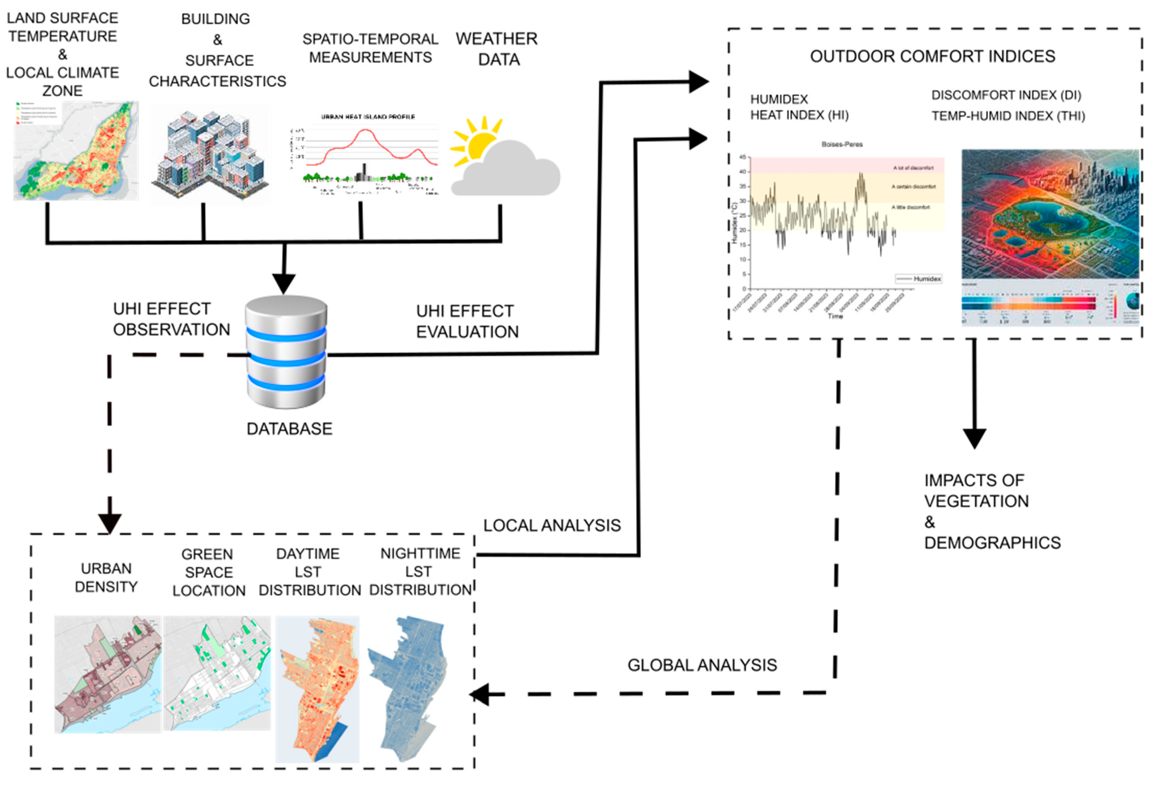
2.1. Methodology
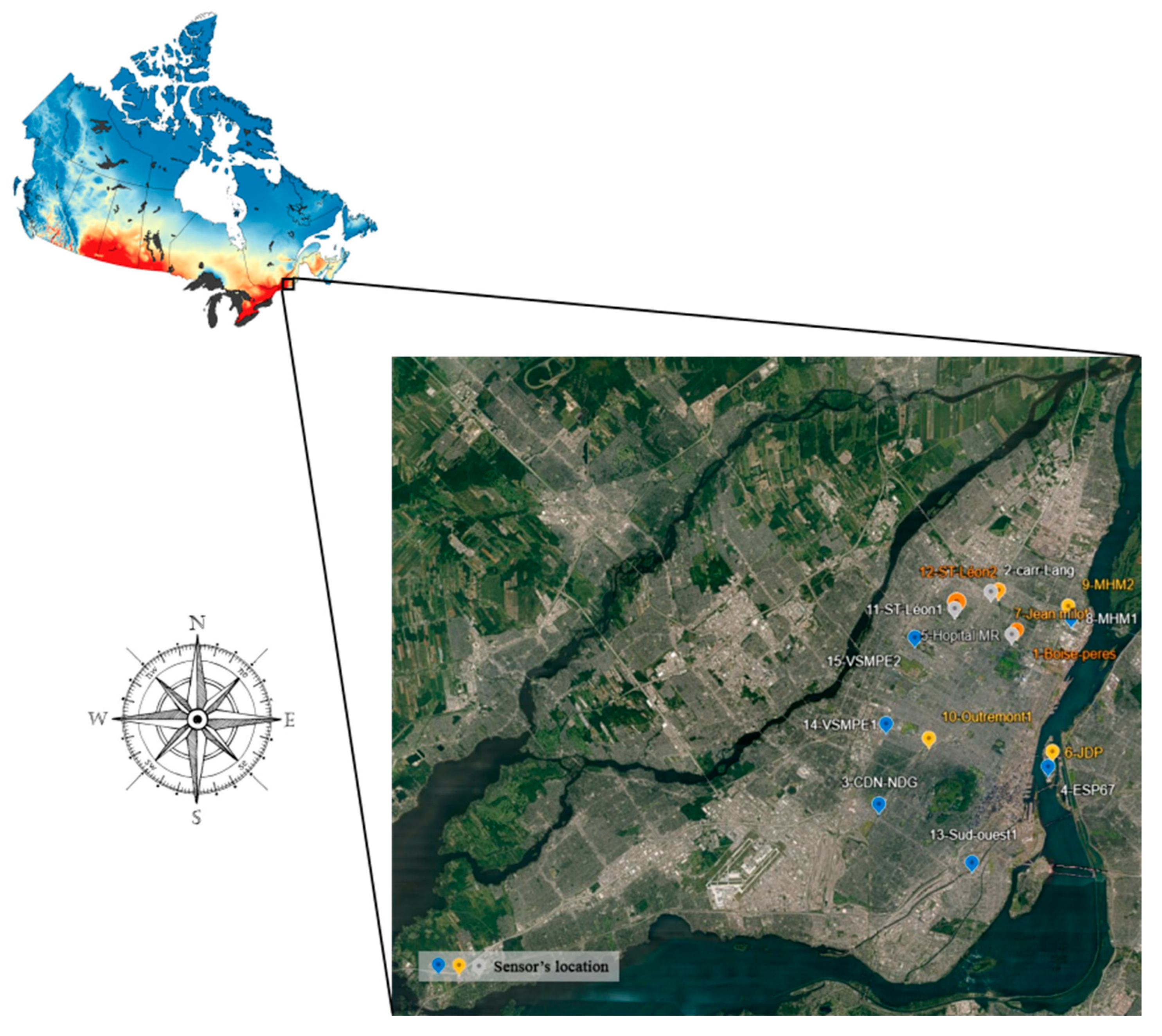
2.2. Data Collection
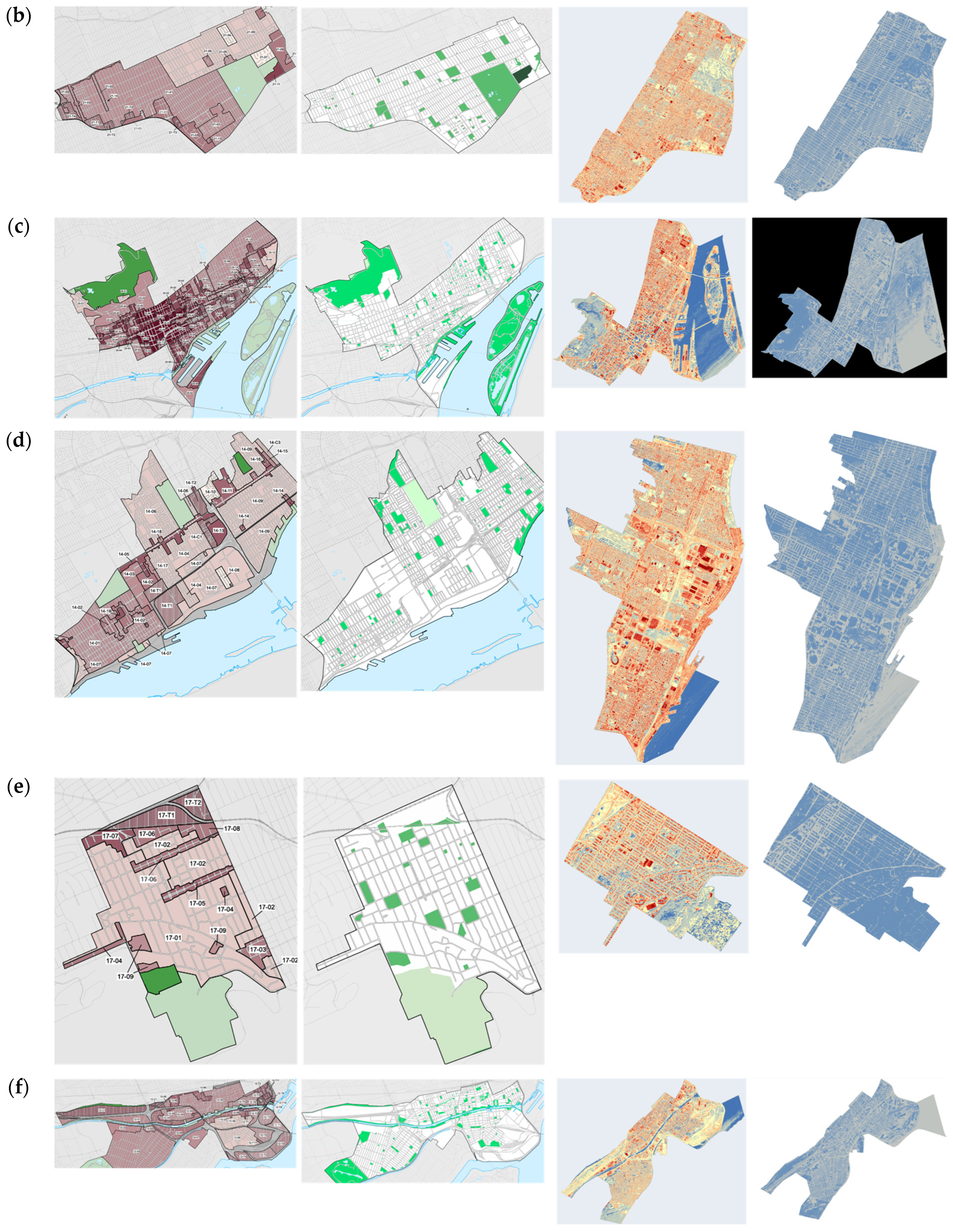
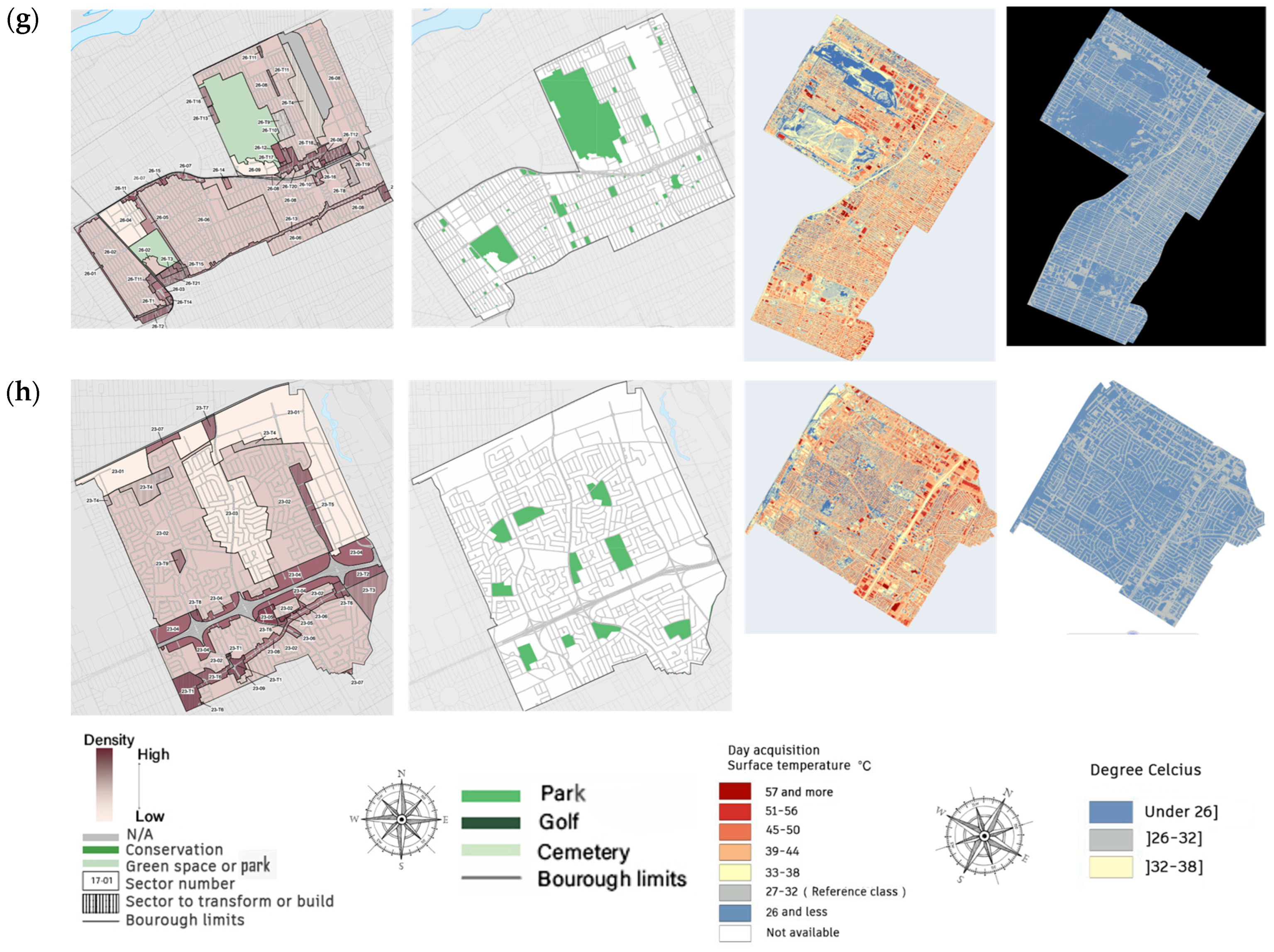
3. Spatial Patterns of UHI-Contributing Factors: Human Thermal Exposure and Discomfort
4. Conclusions and Work Limitations
Author Contributions
Funding
Data Availability Statement
Conflicts of Interest
Nomenclature
| Abbreviations | SVF | Sky View Factor | |
| UHI | Urban Heat Island | BEM | Building Energy Model |
| LST | Land surface temperature | WRF | Weather Research and Forecasting |
| UHI | Urban Heat Island | POS | Percentage of Synchronization |
| SUHII | Surface UHI intensity | Symbols | |
| HW | Heat wave | e | Vapor pressure (hPa) |
| DHW | Dry heat wave | k | The number of factors |
| MHW | Moist heat wave | RH | Relative humidity (%) |
| EHY | Extreme heat years | T | Air temperature (°C) |
| CDH | Cooling degree hours | Dew point temperature (°C) | |
| LCZ | Local climate zone | Tw | Wet-bulb temperature (°C) |
| EHDE | Extra Hot Day Exposure | Time (days) | |
Appendix A. List of Indices

| Index | Formula | Description |
|---|---|---|
| Percentage of synchronisation (POS) [15] | This index serves the purpose of selecting a representative EHY based on the idea of synchronization of the outdoor and indoor extreme years: c = number of extreme years m = number of building configurations i = building configuration VO = (1 or 0) extreme outdoor year in the indoor extreme.year. | |
| Temperature based index (severity) [15] | This index calculates the severity of the heat event by weighting the number of cooling degree hours. = the hourly daily operative temperature = the adaptive threshold temperature | |
| Thermal based index (severity) [15] | This index calculates the severity of the heat event. N = duration in days of heat event = severity during daytime = severity during nightime = standart effective temperature (confort index) surpass 4C for two successive days, it’s a heat event. | |
| Rural-ring [14] | The UHI is calculated as the temperature difference between urban areas and surrounding rural areas | |
| Urban-increment [14] | The UHI is calculated as the temperature between the urban land-cover of the cities and another in which the urban land-cover is replaced by croplands | |
| Actual moisture availability [14] | (θ) = The volumetric soil moisture in the top surface layer Fvegetation = the average green area fraction | |
| Surface energy balance [14] | The net amount of income and outcome energy of a wave can be split into three parts, including the sensible heat flux (QH), latent heat flux (QE), and net heat storage flux (ΔQS) | |
| Cooling degree-hours [16] | CDH refers to the extent of cooling demand in degree hours for a chosen base temperature and is defined as the cumulative sum of the temperature difference between the hourly outside reference and base temperature Ti = hourly temperature (°C), Tb = base temperature (°C), = 0, when Ti < Tb | |
| Surface UHI intensity [11] | ||
| Relationship between the SUHI and the independent parameters [11] | NDBI is the mean brightness, NDVI is the mean greenness, NDWI is the mean wetness in urban areas. Distance is the Euclidean distance of the city center from the coastline. Density is the population density of each city. | |
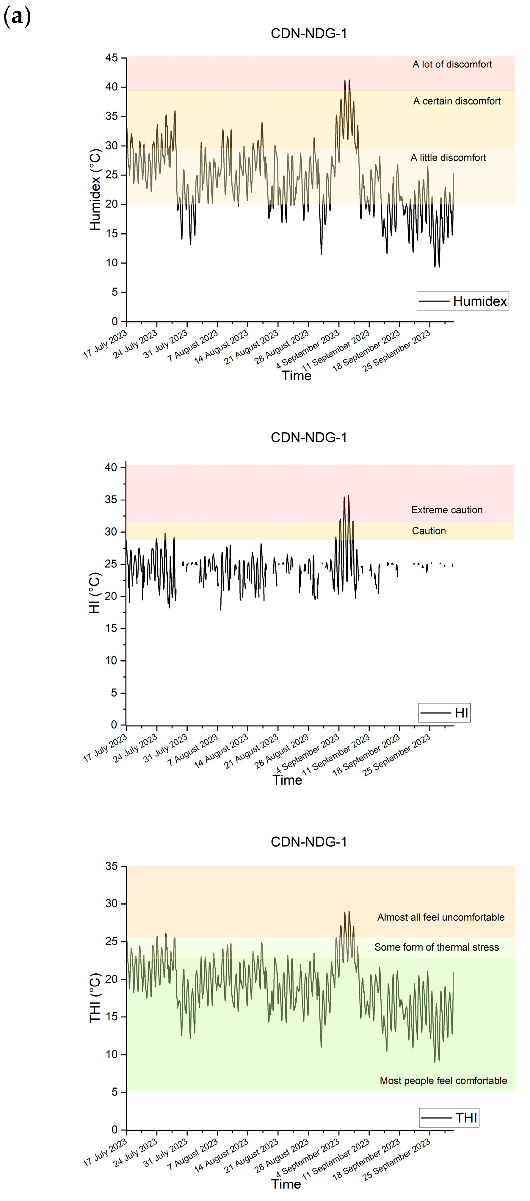
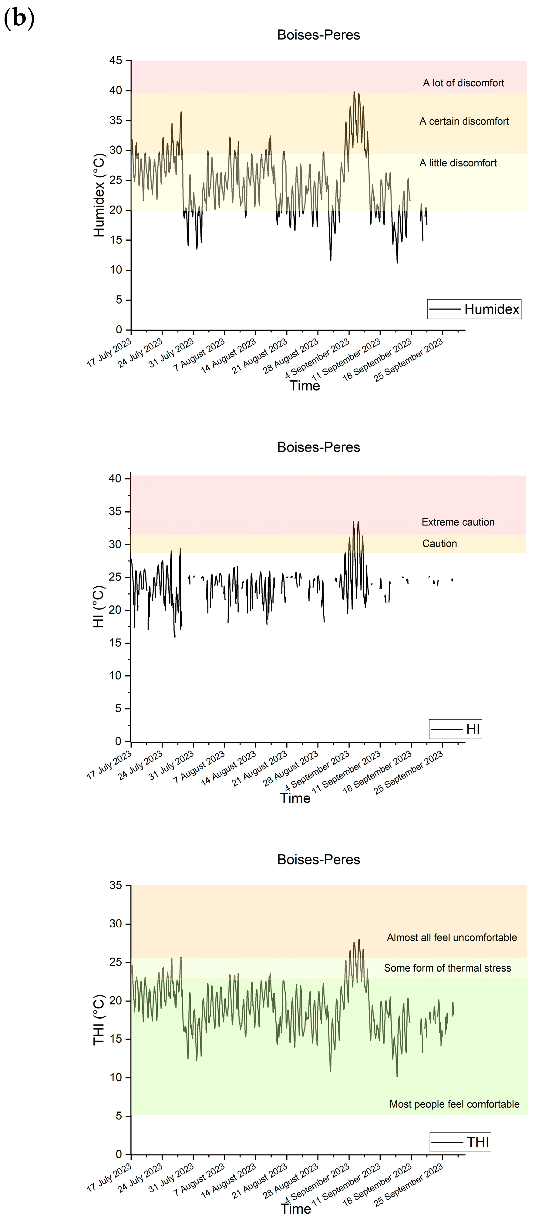
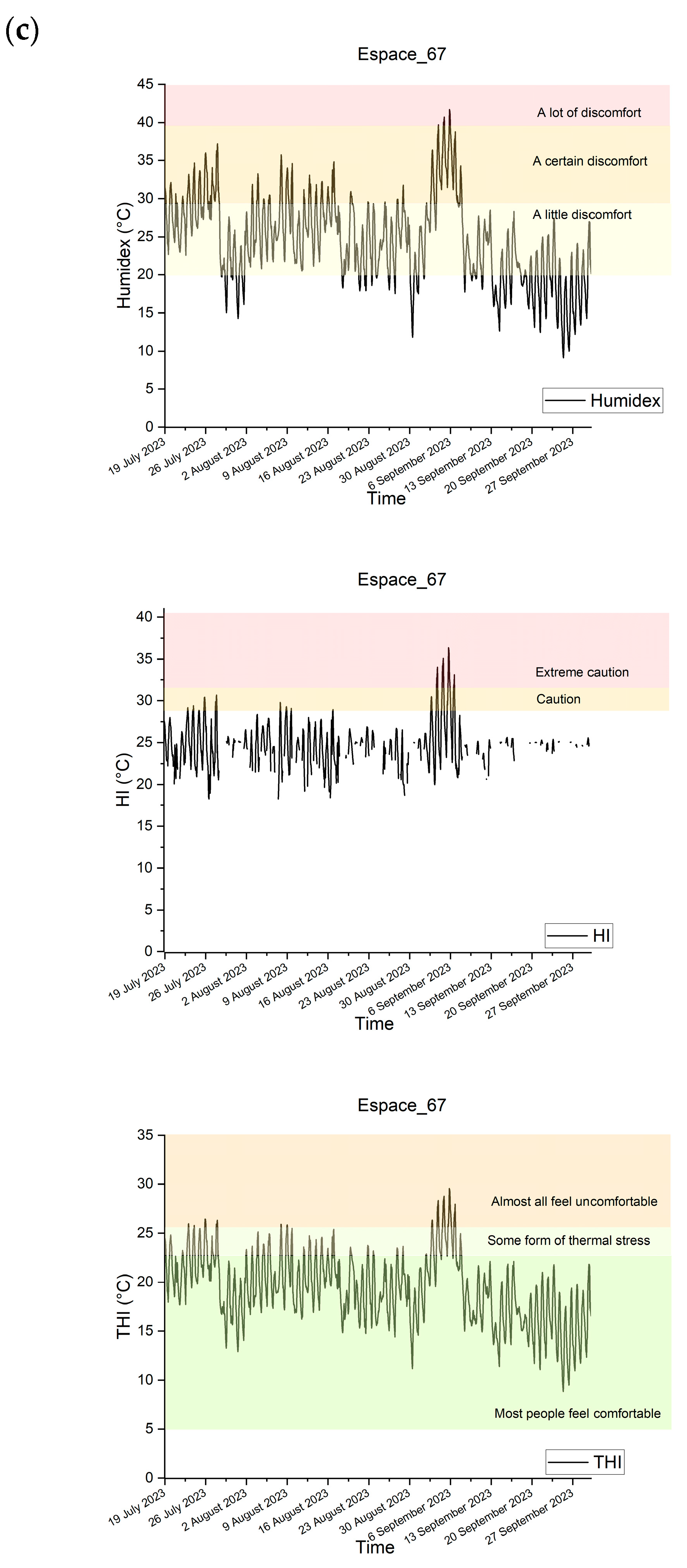
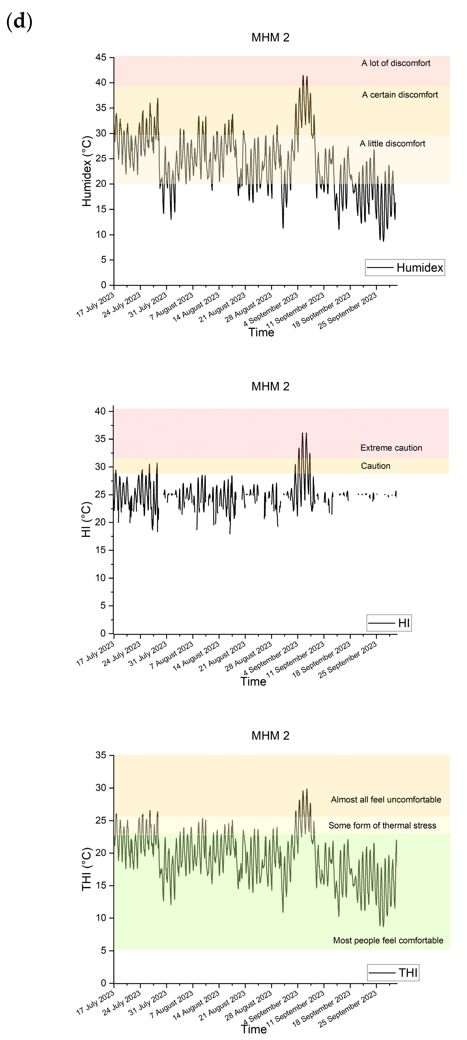
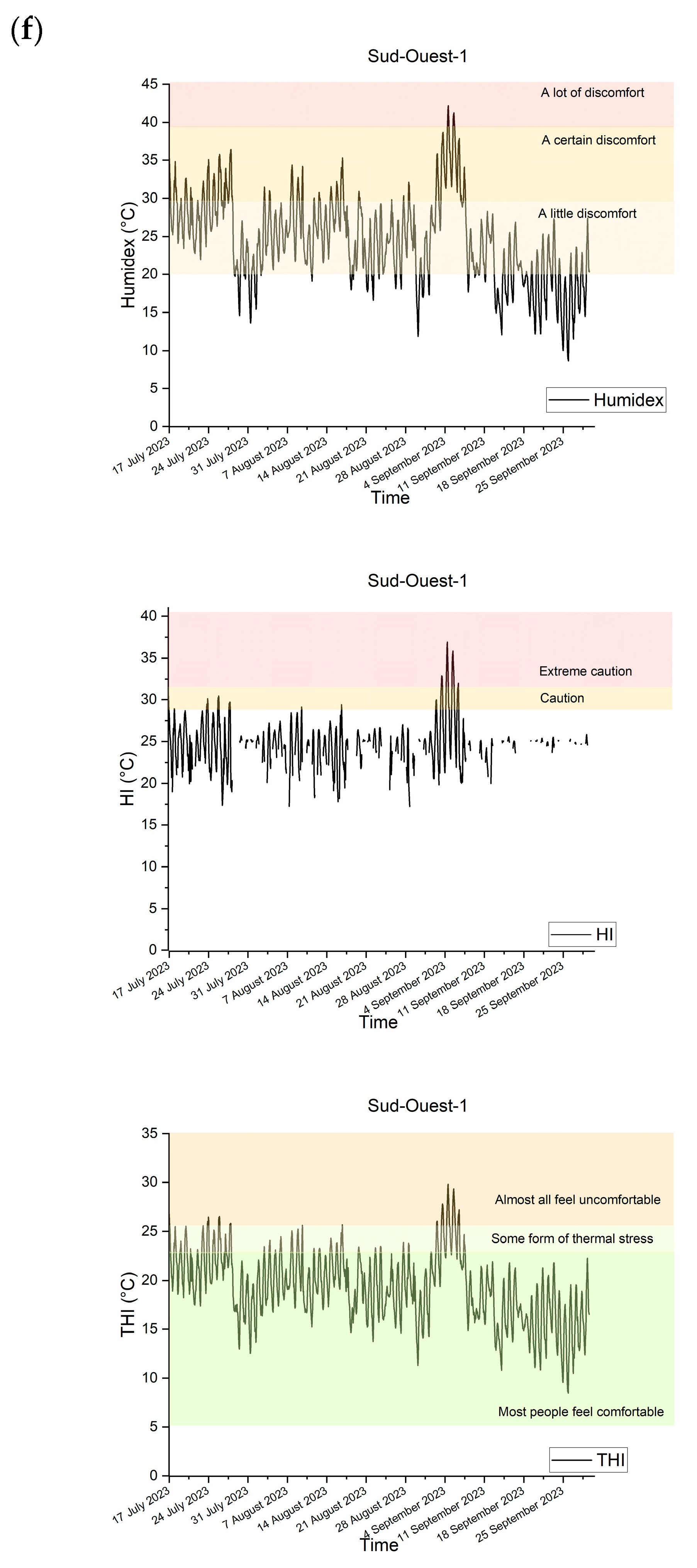
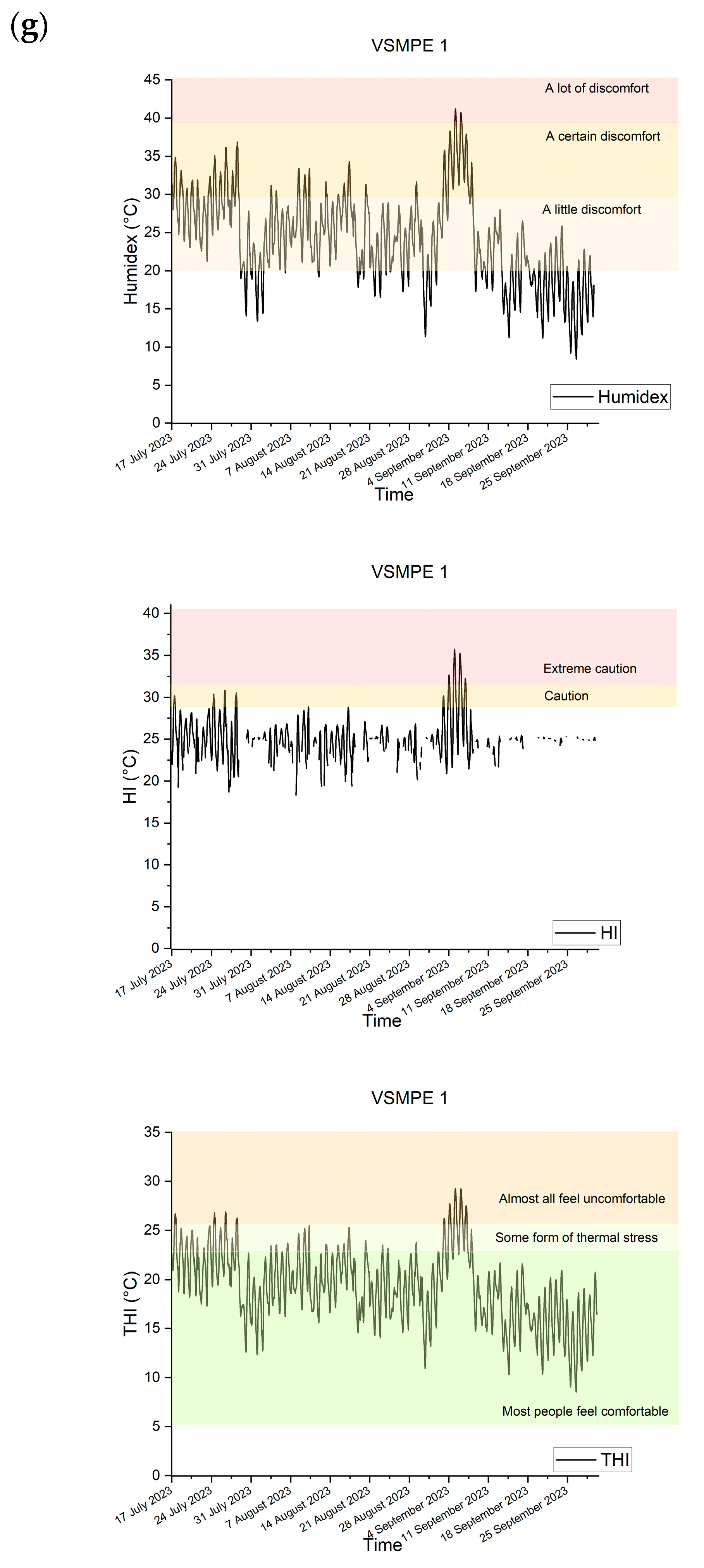
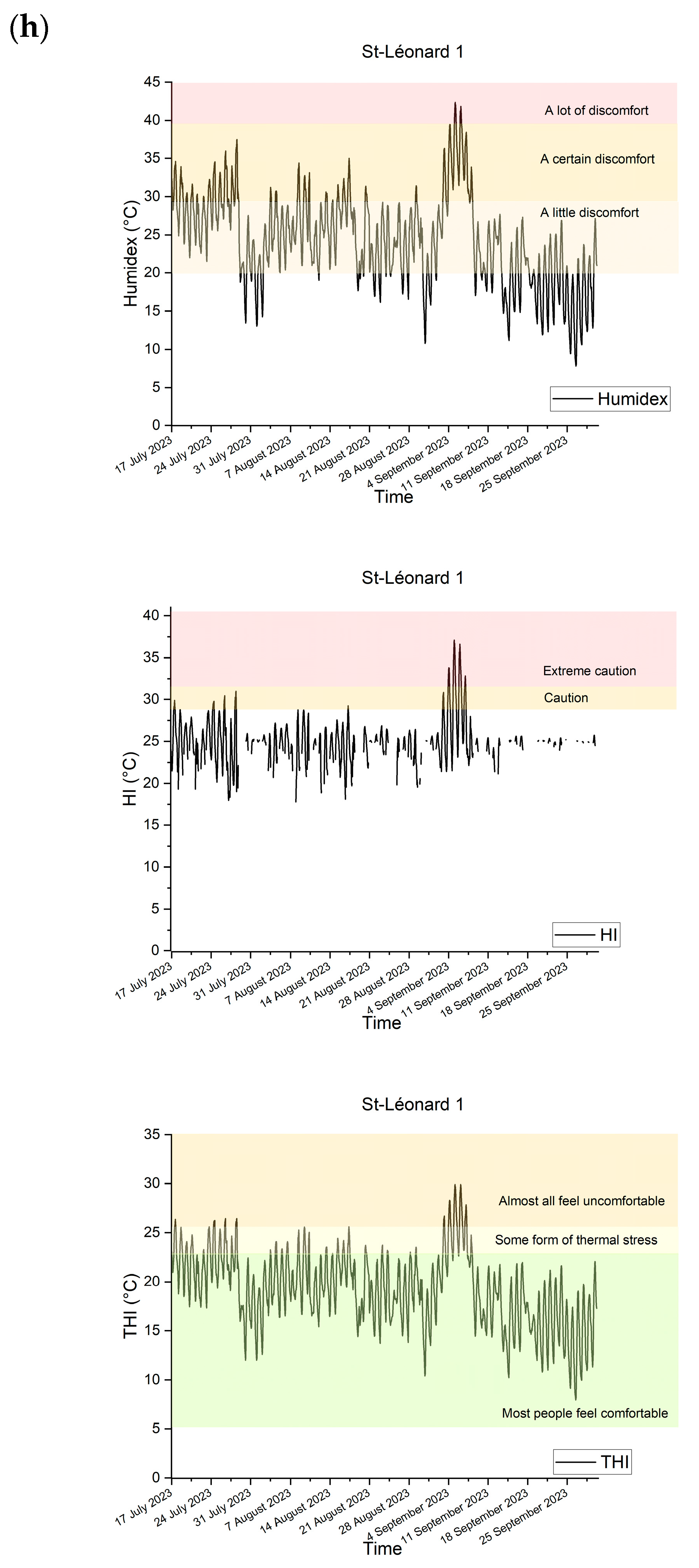
| Humidex [33] | e = Vaport pressure (hPa): Dew point is expressed in kelvins (temperature en K = temperature in °C + 273.15) | From 20 to 29: A little discomfort. From 30 to 39: Some discomfort. From 40 to 45: A lot of discomfort; avoid effort. Above 45: Danger; possible heat stroke [34]. |
| Wet-bulb temperature (Tw) [13] | ||
| Disconfort index [13] | Under 22: No heat stress is encountered. 22–24: Most people feel a mild sensation of heat. 24–28: The heat load is moderately heavy, people feel very hot, and physical work may be performed with some difficulties. Above 28: The heat load is considered severe, and people engaged in physical work are at increased risk for heat illness [26]. | |
| Heat index [4] A corriger | Relative humidity (RH, %): 27–32: Caution; Fatigue possible with prolonged exposure and/or physical activity. 32–41: Extreme caution; Sunstroke, muscle cramps, and/or heat exhaustion possible with prolonged exposure and/or physical activity. 41–54: Danger; Sunstroke, muscle cramps, and/or heat exhaustion likely. Heatstroke possible with prolonged exposure and/or physical activity. ≥54: Extreme danger; Heat stroke or sunstroke likely [25]. | |
| Hot day exposure [8] | is the hot-day exposure of point i, is the annual number of hot days at point i, POPi is the population of point i. | |
| Poverty related heat exposure [8] | ||
| Extra heat day exposure [17] | ||
| The sum of EHDE [17] | Total EHDE due to the UHI effect is estimated as the sum of the EHDE for all built-type LCZs | |
| EHDE intensity [17] | The EHDE intensity of LCZ, ILCZj, is defined as the ratio of EHDE to area in the LCZj | |
| Integral Index of Connectivity (IIC) [26] | The Integral Index of IIC and PC serve to gauge the thermal landscape connectivity of UHI sources. dI index serves to identify crucial heat sources. n = the total number of heat source patches; = represent the area of patches; is the total area of the landscape research area; I = the connectivity index value when the landscape contains landscape elements; = is the index value after removing the landscape element. | |
| Probability of Connectivity (PC) [26] | ||
| Patch importance (dI) [26] | ||
| Plan area density [25] | This index helps calculate the SVF on 2d plans Hm = building height, plan area density, frontal area density, b = building size, w = street width. | |
| Frontal area density [25] | ||
| Calculating Sky view factor [25] | F1 = is the sum of street-to-wall view factors (Frw) subtracted from unity, h = the wall height and w is the street width. | |
| Temperature-humidity index (THI) [30] | This index helps determine the effect of relative humidity and air temperature on thermal comfort. THI of about 21 °C is associated with most people feeling comfortable; at a THI of about 24 °C around half of the population experiences some form of thermal stress; when THI reaches 26 °C, almost all feel uncomfortable [37]. |
Appendix B. Demographic Distribution
| Borough | Population in 2021 | Variation (%) 2016–2021 | Area (km2) | Density (hab./km2) |
|---|---|---|---|---|
| MONTREAL AGGLOMERATION | 2,004,265 | 3.20 | 498.29 | 4022 |
| City of Montreal | 1,762,949 | 3.42 | 364.74 | 4834 |
| Ahuntsic–Cartierville | 135,336 | 0.81 | 24.16 | 5602 |
| Anjou | 43,243 | 1.04 | 13.68 | 3161 |
| Côte-des-Neiges–Dame-de-Grâce | 170,583 | 2.44 | 21.44 | 7956 |
| Lachine | 46,428 | 4.36 | 17.72 | 2620 |
| LaSalle | 82,235 | 7.00 | 16.27 | 5054 |
| Plateau–Mont-Royal | 105,813 | 1.74 | 8.13 | 13,015 |
| Sud-Ouest | 84,553 | 8.19 | 15.68 | 5392 |
| L’Île-Bizard–Sainte-Geneviève | 18,885 | 2.56 | 23.60 | 800 |
| Mercier–Hochelaga–Maisonneuve | 140,627 | 3.38 | 25.41 | 5534 |
| Montreal-Nord | 88,471 | 5.03 | 11.05 | 8006 |
| Outremont | 24,629 | 2.82 | 3.85 | 6397 |
| Pierrefonds–Roxboro | 70,382 | 1.57 | 27.06 | 2601 |
| Rivière-des-Prairies–Pointe-aux-Trembles | 107,941 | 1.12 | 42.28 | 2553 |
| Rosemont–La-Petite-Patrie | 141,813 | 1.59 | 15.85 | 8947 |
| Saint-Laurent | 102,104 | 3.31 | 42.77 | 2387 |
| Saint-Léonard | 79,495 | 1.52 | 13.49 | 5893 |
| Verdun | 70,377 | 1.66 | 9.72 | 7244 |
| Ville-Marie | 104,944 | 17.69 | 16.52 | 6353 |
| Villeray–Saint-Michel–Parc-Extension | 145,090 | 0.86 | 16.49 | 8799 |
| City of Baie-D’Urfé | 3764 | −1.54 | 6.01 | 626 |
| City of Beaconsfield | 19,277 | −0.24 | 10.98 | 1756 |
| City of Côte-Saint-Luc | 34,504 | 6.34 | 6.94 | 4972 |
| City of Dollard-des-Ormeaux | 48,403 | −1.01 | 15.17 | 3191 |
| City of Dorval | 19,302 | 1.70 | 20.85 | 926 |
| City of Hampstead | 7037 | 0.92 | 1.79 | 3940 |
| City of Kirkland | 19,413 | −3.66 | 9.62 | 2017 |
| City of Montreal-Est | 4394 | 14.13 | 12.46 | 353 |
| City of Montreal-Ouest | 5115 | 1.29 | 1.40 | 3643 |
| City of Mont-Royal | 20,953 | 3.34 | 7.65 | 2741 |
| City of Pointe-Claire | 33,488 | 6.72 | 18.84 | 1777 |
| City of Sainte-Anne-de-Bellevue | 5027 | 1.39 | 10.55 | 476 |
| City of Senneville | 951 | 3.26 | 7.47 | 127 |
| City of Westmount | 19,658 | −3.22 | 4.02 | 4892 |
Appendix C. Demographic Distribution
| Borough | Population in 2021 | Density (hab/km2) | Vegetation Cover (%) | Sensors | Proximity to the Coast (km) |
|---|---|---|---|---|---|
| Côte-des-Neiges–Notre-Dame-de-Grâce | 170,583 | 7956 | 9.88 | 3-CDN-NDG-1 | 6.6 |
| Rosemont–La-Petite-Patrie | 141,813 | 8947 | 15.24 | 1-Boise-Peres | 3.2 |
| 5-Hopital_M-R | 3.3 | ||||
| Ville-Marie: Sainte-Hélène Island | N/A | N/A | 70.54 | 4-Espace_67 | 0.16 |
| 6-Jean-Drapeau_Etang | 0.14 | ||||
| Mercier–Hochelaga–Maisonneuve | 140,627 | 5534 | 8.27 | 7-Jean-Milot | 4.6 |
| 8-MHM 1 | 1.0 | ||||
| 9-MHM 2 | 1.3 | ||||
| Outremont | 24,629 | 6397 | 24.5 | 10-Outremont 1 | 5.5 |
| Le Sud-Ouest | 84,553 | 5392 | 11.37 | 13-Sud-Ouest-1 | 2.1 |
| Villeray–Saint-Michel–Parc-Extension | 145,090 | 8799 | 14.66 | 14-VSMPE 1 | 3.4 |
| 15-VSMPE 2 | 2.5 | ||||
| Saint-Léonard | 79,495 | 5893 | 5.05 | 11-St-Léonard 1 | 3.8 |
| 12-St-Léonard 2 | 3.8 | ||||
| 2-Carref_Langelier | 5.0 |
References
- Manoli, G.; Fatichi, S.; Schlapfer, M.; Yu, K.L.; Crowther, T.W.; Meili, N.; Burlando, P.; Katul, G.G.; Zeid, E.B. Magnitude of urban heat islands largely explained by climate and population. Nature 2019, 573, 55–60. [Google Scholar] [CrossRef] [PubMed]
- Santamouris, M. On the energy impact of urban heat island and global warming on buildings. Energy Build. 2014, 82, 100–113. [Google Scholar] [CrossRef]
- He, B.J.; Zhao, D.X.; Dong, X.; Xiong, K.; Feng, C.; Qi, Q.L.; Darko, A.; Sharifi, A.; Pathak, M. Perception, physiological and psychological impacts, adaptive awareness and knowledge, and climate justice under urban heat: A study in extremely hot-humid Chongqing. China. Sustain. Cities Soc. 2022, 79, 103685. [Google Scholar] [CrossRef]
- Fadhil, M.; Hamoodi, M.N.; Ziboon, A.R.T. Mitigating urban heat island effects in urban environments: Strategies and tools. IOP Conf. Ser. Earth Environ. Sci. 2023, 1129, 012025. [Google Scholar] [CrossRef]
- Guo, C.; Lanza, K.; Li, D.; Zhou, Y.; Aunan, K.; Loo, B.P.Y.; Lee, J.K.W.; Luo, B.; Duan, X.; Zhang, W.; et al. Impact of heat on all-cause and cause-specific mortality: A multi-city study in Texas. Environ. Res. 2023, 224, 115453. [Google Scholar] [CrossRef]
- Ignjaˇcevi´c, P.; Botzen, W.; Estrada, F.; Daanen, H.; Lupi, V. Climate-induced mortality projections in Europe: Estimation and valuation of heat-related deaths. Int. J. Disaster Risk Reduct. 2024, 111, 104692. [Google Scholar] [CrossRef]
- Mitchell, D. Climate attribution of heat mortality. Nat. Clim. Chang. 2021, 11, 467–468. [Google Scholar] [CrossRef]
- Debbage, N.; Shepherd, J.M. The urban heat island effect and city contiguity. Comput. Environ. Urban Syst. 2015, 54, 181–194. [Google Scholar] [CrossRef]
- Qian, Y.; Chakraborty, T.C.; Li, J.F.; Li, D.; He, C.L.; Sarangi, C.; Chen, F.; Yang, X.C.; Leung, L.R. Urbanization impact on regional climate and extreme weather: Current understanding, uncertainties, and future research directions. Adv. Atmos. Sci. 2022, 39, 819–860. [Google Scholar] [CrossRef]
- Oke, T.R. The energetic basis of the UHI. Q. J. R. Meteorol. Soc. 1982, 108, 1–24. [Google Scholar]
- Firozjaei, M.K.; Sedighi, A.; Mijani, N.; Kazemi, Y.; Amiraslani, F. Seasonal and daily effects of the sea on the surface UHI intensity: A case study of cities in the Caspian Sea Plain. Urban Clim. 2023, 51, 101603. [Google Scholar] [CrossRef]
- Zhao, L.; Oppenheimer, M.; Zhu, Q.; Baldwin, J.W.; Ebi, K.L.; Bou-Zeid, E.; Guan, K.; Liu, X. Interactions between UHIs and heat waves. Environ. Res. Lett. 2018, 13, 034003. [Google Scholar] [CrossRef]
- Kim, D.-H.; Park, K.; Baik, J.-J.; Jin, H.-G.; Han, B.-S. Contrasting interactions of UHIs with dry and moist heat waves and their implications for urban heat stress. Urban Clim. 2024, 56, 102050. [Google Scholar] [CrossRef]
- Shu, C.; Gaur, A.; Wang, L.; Lacasse, M. Evolution of the local climate in Montreal and Ottawa before, during and after a heatwave and the effects on UHIs. Sci. Total Environ. 2023, 890, 164497. [Google Scholar] [CrossRef]
- Ji, L.; Laouadi, A.; Shu, C.; Gaur, A.; Lacasse, M.; Wang, L. Evaluating approaches of selecting extreme hot years for assessing building overheating conditions during heatwaves. Energy Build. 2022, 245, 111610. [Google Scholar] [CrossRef]
- Errebai, F.B.; Strebel, D.; Carmeliet, J.; Derome, D. Impact of UHI on cooling energy demand for residential building in Montreal using meteorological simulations and weather station observations. Energy Build. 2022, 273, 112410. [Google Scholar] [CrossRef]
- Yu, W.; Yang, J.; Sun, D.; Ren, J.; Xue, B.; Sun, W.; Xiao, X.; Xia, J.C.; Li, X. How UHI magnifies hot day exposure: Global unevenness derived from differences in built landscape. Sci. Total Environ. 2024, 945, 174043. [Google Scholar] [CrossRef]
- Alizadeh, M.R.; Abatzoglou, J.T.; Adamowski, J.F.; Prestemon, J.P.; Chittoori, B.; Akbari Asanjan, A.; Sadegh, M. Increasing heat-stress inequality in a warming climate. Earth’s Future 2022, 10, e2021EF002488. [Google Scholar] [CrossRef]
- Tuholske, C.; Caylor, K.; Funk, C.; Verdin, A.; Sweeney, S.; Grace, K.; Peterson, P.; Evans, T. Global urban population exposure to extreme heat. Proc. Natl. Acad. Sci. USA 2021, 118, e2024792118. [Google Scholar] [CrossRef]
- Wang, Y.; Zhao, N.; Yin, X.; Wu, C.; Chen, M.; Jiao, Y.; Yue, T. Global future population exposure to heatwaves. Environ. Int. 2023, 178, 108049. [Google Scholar] [CrossRef]
- Stewart, I.; Oke, T. Local climate zones for urban temperature studies. Bull. Am. Meteorol. Soc. 2012, 93, 1879–1900. [Google Scholar] [CrossRef]
- Welegedara, N.P.Y.; Agrawal, S.K.; Lotfi, G. Exploring spatiotemporal changes of the UHI effect in high-latitude cities at a neighbourhood level: A case of Edmonton, Canada. Sustain. Cities Soc. 2023, 90, 104403. [Google Scholar] [CrossRef]
- Hurduc, A.; Ermida, S.L.; Trigo, I.F.; DaCamara, C.C. Importance of temporal dimension and rural land cover when computing surface UHI intensity. Urban Clim. 2024, 56, 102013. [Google Scholar] [CrossRef]
- Deng, X.; Yu, W.; Shi, J.; Huang, Y.; Li, D.; He, X.; Zhou, W.; Xie, Z. Characteristics of surface UHIs in global cities of different scales: Trends and drivers. Sustain. Cities Soc. 2024, 107, 105483. [Google Scholar] [CrossRef]
- Touchaei, A.G.; Wang, Y. Characterizing UHI in Montreal (Canada)—Effect of urban morphology. Sustain. Cities Soc. 2015, 19, 395–402. [Google Scholar] [CrossRef]
- Zhao, Z.; Li, W.; Zhang, J.; Zheng, Y. Constructing an UHI network based on connectivity perspective: A case study of Harbin, China. Ecol. Indic. 2024, 159, 111665. [Google Scholar] [CrossRef]
- Shamsaei, M.; Carter, A.; Vaillancourt, M. Using urban and demolition waste materials to alleviate the negative effect of pavements on the UHI: A laboratory, field, and numerical study. Case Stud. Urban Mater. 2024, 20, e03346. [Google Scholar]
- Ghaseminasab, M.; Berraha, Y.; Carter, A.; Vaillancourt, M. Caractérisation des paramètres thermiques de mélanges d’enrobé bitumineux contenant différents matériaux de post-consommation, à l’aide de deux méthodes d’essai thermique. Via Bitume 2023, 18, 46–51. [Google Scholar]
- Faragallah, R.N.; Ragheb, R.A. Evaluation of thermal comfort and UHI through cool paving materials using ENVI-Met. Ain Shams Eng. J. 2022, 13, 101609. [Google Scholar] [CrossRef]
- Cortes, A.; Rejuso, A.J.; Santos, J.A.; Blanco, A. Evaluating mitigation strategies for UHI in Mandaue City using ENVI-met. J. Urban Manag. 2022, 11, 97–106. [Google Scholar] [CrossRef]
- Morales-Gonzalez, I.; Verichev, K.; Carpio, M. Efficiency assessment for the UHI mitigation measures in a city with an oceanic climate during the summer period: Case of Valdivia, Chile. Urban Clim. 2024, 55, 101897. [Google Scholar] [CrossRef]
- Zhao, Q.; Tao, L.; Song, H.; Lin, Y.; Ji, Y.; Geng, J.; Liu, J. Mitigation pathways of urban heat islands and simulation of their effectiveness from a perspective of connectivity. Sustain. Cities Soc. 2025, 124, 106300. [Google Scholar] [CrossRef]
- Masterton, J.M.; Richardson, F.A. Humidex A. Method of Quantifying Human Discomfort Due to Excessive Heat and Humidity; Environment Canada: Downsview, ON, Canada, 1979. [Google Scholar]
- Canadian Centre for Occupational Health and Safety. Available online: https://www.ccohs.ca/oshanswers/phys_agents/humidex.html (accessed on 10 November 2024).
- Blazejczyk, K.; Epstein, Y.; Jendritzky, G.; Staiger, H.; Tinz, B. Comparison of UTCI to selected thermal indices. Int. J. Biometeorol. 2012, 56, 515–535. [Google Scholar] [CrossRef] [PubMed]
- Epstein, Y.; Moran, D.S. Thermal Comfort and the Heat Stress. Ind. Health 2006, 44, 388–398. [Google Scholar] [CrossRef]
- Lia, X.-X.; Norford, L.K. Evaluation of cool roof and vegetations in mitigating UHI in a tropical city, Singapore. Urban Clim. 2015, 16, 59–74. [Google Scholar] [CrossRef]
- Available online: https://www.thecanadianencyclopedia.ca/fr/article/montreal-1 (accessed on 15 November 2024).
- Available online: https://donnees.montreal.ca/dataset (accessed on 10 November 2024).
- Available online: https://www.onsetcomp.com/ (accessed on 16 November 2024).
- Available online: http://ville.montreal.qc.ca/portal/ (accessed on 16 November 2024).
- Available online: https://www.canada.ca/fr/environnement-changement-climatique/services/changements-climatiques/centre-canadien-services-climatiques/afficher-telecharger/documentation-technique-normales-climatiques.html (accessed on 7 October 2024).
- Available online: https://bter.maps.arcgis.com/apps/webappviewer/index.html?id=157cde446d8942d7b4367e2159942e05 (accessed on 7 January 2024).


| Station’s Name | Geographical Location | Sensor Coordinates | |
|---|---|---|---|
| Longitude | Latitude | ||
| 1-Boise-Peres | Rosemont-La Petite-Patrie | −73.556306 | 45.57569 |
| 2-Carref_Langelier | Saint-Léonard | −73.573583 | 45.59319 |
| 3-CDN-NDG-1 | Côte-des-Neiges-Notre-Dame-de-Grâce | −73.648944 | 45.49355 |
| 4-Espace_67 | Ville-Marie | −73.535417 | 45.51102 |
| 5-Hopital_M-R | Rosemont-La Petite-Patrie | −73.559639 | 45.57333 |
| 6-Jean-Drapeau_Etang | Ville-Marie | −73.532472 | 45.51802 |
| 7-Jean-Milot | Mercier-Hochelaga-Maisonneuve | −73.568444 | 45.59394 |
| 8-MHM 1 | Mercier-Hochelaga-Maisonneuve | −73.519722 | 45.58097 |
| 9-MHM 2 | Mercier-Hochelaga-Maisonneuve | −73.521556 | 45.58633 |
| 10-Outremont 1 | Outremont | −73.615361 | 45.52438 |
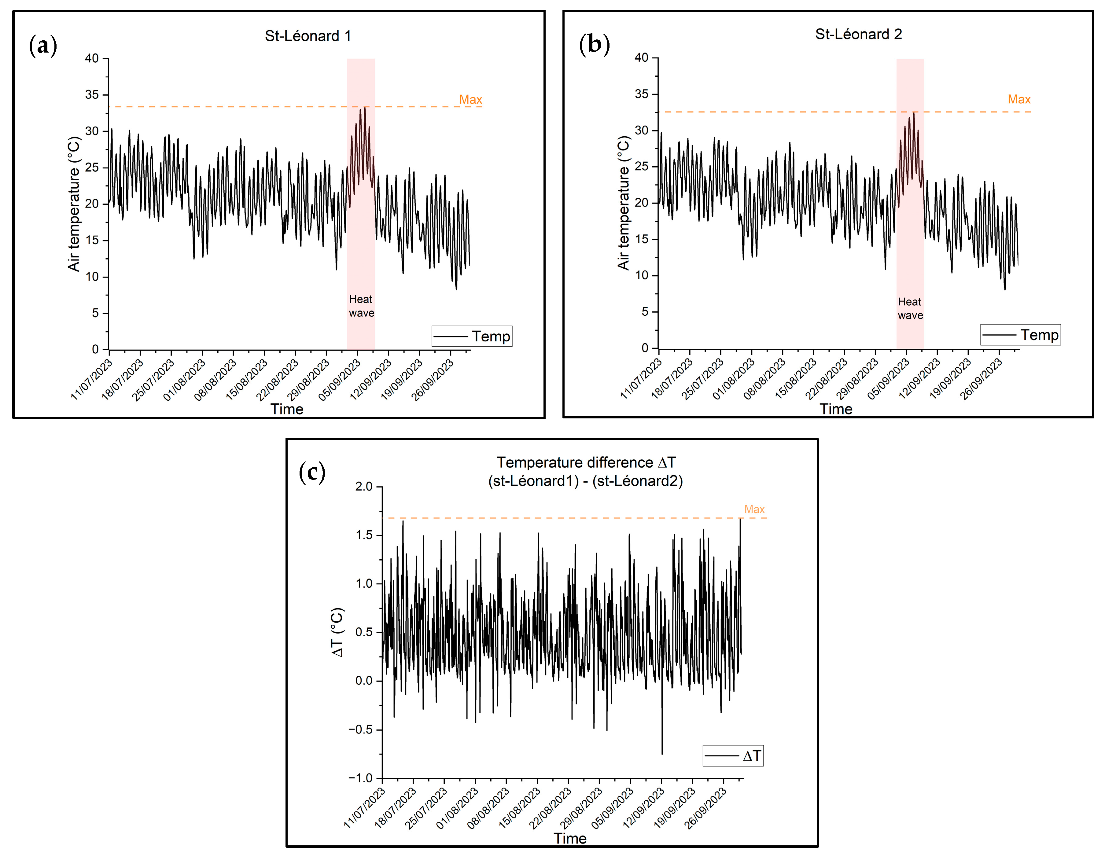
| 11-Saint-Léonard 1 | Saint-Léonard | −73.597917 | 45.58536 |
| 12-Saint-Léonard 2 | Saint-Léonard | −73.596472 | 45.58630 |
| 13-Sud-Ouest-1 | Le Sud-Ouest | −73.586583 | 45.46594 |
| 14-VSMPE 1 | Villeray-Saint-Michel-Parc-Extension | −73.644056 | 45.53125 |
| 15-VSMPE 2 | Villeray-Saint-Michel-Parc-Extension | −73.624667 | 45.57175 |
| Specifications | Values |
|---|---|
| Acquisition period | 3 August to 3 September 2016 |
| Wind direction | 130° |
| Average wind speed | 16 km/h |
| Average air temperature on 20 August 2016 | 28.9 °C |
| Thermal sensor | TASI 600 (8–12 μm) |
| Image resolution | 2 m/pixel |
| Planimetric accuracy of thermography | ±2.3 m |
| Thermal measurement accuracy | ±3 °C |
| Instrument | Image | Operating Range | Accuracy | Objective |
|---|---|---|---|---|
| Onset HOBO MICRO (RX2102) |  | −4 to 140 °F (−20 to 60 °C) | ±8 s per month in 32 to 104 °F (0 to 40 °C) range ±30 s per month in −40 to 140 °F (−40 to 60 °C) range | Saving obtained data |
| Smart Sensors (S-THB-M002) | 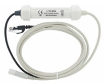 | −40 °C to 75 °C (−40 °F to 167 °F) | ±0.21 °C from 0° to 50 °C (±0.38 °F from 32 to 122 °F) | Measuring relative humidity and air temperature |
| Ville Marie | Whole Borough | Coastal City | Sainte-Hélène Island | Notre Dame Island |
|---|---|---|---|---|
| Vegetation cover (%) | 24.39 | 17.77 | 70.54 | 47.26 |
| Water body cover (%) | - | - | 6.86 | 32.89 |
| Comfort Index | Threshold | Impact |
|---|---|---|
| Humidex | 40 | The population experiences a lot of discomfort and should avoid heavy exertion. |
| DI | 24 | The thermal load is moderately high, people feel very hot, and physical work can be performed with some difficulty. |
| HI | 32 | People need to be extremely cautious. There is a possibility of sunstroke, muscle cramps, and heat exhaustion in cases of prolonged exposure and/or physical activity. |
| THI | 26 | Almost everyone feels uncomfortable. |
| Station’s Name | Period | Exceedance in % | |||
|---|---|---|---|---|---|
| Humidex > 40 | DI > 24 | HI > 32 | THI > 26 | ||
| 1-Boise-Peres | NHW | 0.00 | 4.13 | 0.88 | 1.75 |
| HW | 0.00 | 43.33 | 11.67 | 23.33 | |
| 2-Carref_Langelier | NHW | 0.33 | 5.25 | 1.31 | 2.90 |
| HW | 5.00 | 48.33 | 20.00 | 34.17 | |
| 3-CDN-NDG-1 | NHW | 0.22 | 2.34 | 0.44 | 1.10 |
| HW | 6.67 | 43.33 | 13.33 | 30.83 | |
| 4-Espace_67 | NHW | 0.40 | 6.36 | 1.25 | 2.27 |
| HW | 5.83 | 45.83 | 18.33 | 26.67 | |
| 5-Hopital_M-R | NHW | 0.61 | 6.07 | 1.54 | 3.09 |
| HW | 9.17 | 50.83 | 23.33 | 34.17 | |
| 6-Jean-Drapeau_Etang | NHW | 0.00 | 3.59 | 0.22 | 1.06 |
| HW | 0.00 | 40.83 | 3.33 | 15.83 | |
| 7-Jean-Milot | NHW | 0.50 | 3.53 | 0.66 | 1.38 |
| HW | 7.50 | 33.33 | 10.00 | 20.83 | |
| 8-MHM 1 | NHW | 0.60 | 6.09 | 1.59 | 3.02 |
| HW | 9.17 | 53.33 | 24.17 | 36.67 | |
| 9-MHM 2 | NHW | 0.55 | 5.76 | 1.54 | 3.02 |
| HW | 8.33 | 50.00 | 23.33 | 36.67 | |
| 10-Outremont 1 | NHW | 0.55 | 5.76 | 1.15 | 2.19 |
| HW | 8.33 | 48.33 | 17.50 | 30.00 | |
| 11-Saint-Leoonard 1 | NHW | 0.71 | 6.41 | 1.48 | 3.02 |
| HW | 10.83 | 50.00 | 22.50 | 35.00 | |
| 12-Saint-Leonard 2 | NHW | 0.44 | 4.99 | 1.15 | 2.19 |
| HW | 6.67 | 45.00 | 17.50 | 30.00 | |
| 13-Sud-Ouest-1 | NHW | 0.61 | 6.08 | 1.16 | 2.82 |
| HW | 9.17 | 45.83 | 17.50 | 31.67 | |
| 14-VSMPE 1 | NHW | 0.38 | 6.36 | 1.26 | 3.29 |
| HW | 5.83 | 50.83 | 19.17 | 32.50 | |
| 15-VSMPE 2 | NHW | 0.60 | 5.32 | 1.21 | 2.41 |
| HW | 9.17 | 48.33 | 18.33 | 34.17 | |
Disclaimer/Publisher’s Note: The statements, opinions and data contained in all publications are solely those of the individual author(s) and contributor(s) and not of MDPI and/or the editor(s). MDPI and/or the editor(s) disclaim responsibility for any injury to people or property resulting from any ideas, methods, instructions or products referred to in the content. |
© 2025 by the authors. Licensee MDPI, Basel, Switzerland. This article is an open access article distributed under the terms and conditions of the Creative Commons Attribution (CC BY) license (https://creativecommons.org/licenses/by/4.0/).
Share and Cite
Hedeya, Y.; Merabtine, A.; Maref, W. Evaluating the Urban Heat Island Effect in Montreal: Urban Density, Vegetation, Demographic, and Thermal Landscape Analysis. Buildings 2025, 15, 1562. https://doi.org/10.3390/buildings15091562
Hedeya Y, Merabtine A, Maref W. Evaluating the Urban Heat Island Effect in Montreal: Urban Density, Vegetation, Demographic, and Thermal Landscape Analysis. Buildings. 2025; 15(9):1562. https://doi.org/10.3390/buildings15091562
Chicago/Turabian StyleHedeya, Yassine, Abdelatif Merabtine, and Wahid Maref. 2025. "Evaluating the Urban Heat Island Effect in Montreal: Urban Density, Vegetation, Demographic, and Thermal Landscape Analysis" Buildings 15, no. 9: 1562. https://doi.org/10.3390/buildings15091562
APA StyleHedeya, Y., Merabtine, A., & Maref, W. (2025). Evaluating the Urban Heat Island Effect in Montreal: Urban Density, Vegetation, Demographic, and Thermal Landscape Analysis. Buildings, 15(9), 1562. https://doi.org/10.3390/buildings15091562