Construction and Recording Method of a Three-Dimensional Model to Automatically Manage Thermal Abnormalities in Building Exteriors

Abstract

This study proposes an automated three-dimensional (3D)-modeling method that combines convolutional neural networks (CNNs) with unmanned aerial vehicle (UAV) technology for the efficient management of thermal anomalies in building exteriors. Conventional 3D-modeling methods for thermal imaging management either require the processing of large volumes of data due to the use of thermal distribution information from entire image regions or involve increased processing time when architectural drawings are unavailable. In this study, RGB and infrared (IR) thermal images collected via UAVs were used to automatically detect windows and thermal anomalies using a CNN-based object detection model (YOLOv5). Subsequently, Global Navigation Satellite System (GNSS)-based coordinate data and image metadata were used to convert the resolution coordinates into actual spatial coordinates, which were then vectorized to automatically generate a 3D model. The resulting 3D model demonstrated high similarity to the actual building, accurately representing the locations of thermal anomalies. This method enabled faster, more objective, and more cost-effective maintenance compared to conventional methods, making it especially beneficial for efficiently managing difficult-to-access high-rise buildings.

1. Introduction

Contemporary buildings have evolved beyond their fundamental role of protecting interiors from external environmental factors; they have now developed into complex systems that integrate energy efficiency and sustainability, encompassing heating, lighting, and other aspects. In particular, the thermal performance of a building’s exterior envelope can be crucial in maintaining a pleasant indoor environment. Moreover, it can directly impact a building’s energy consumption. However, when thermal anomalies—such as reduced thermal performance or thermal bridging—occur in the building envelope, the building’s energy efficiency deteriorates, and prolonged neglect of these problems can increase maintenance costs [1,2]. Consequently, it is essential to establish a maintenance system that can detect and address thermal anomalies in building exteriors at an early stage.

Traditionally, inspectors have used thermal imaging cameras for on-site inspections and indoor temperature monitoring to assess thermal anomalies within buildings [3]. However, this method can present difficulties in data collection for analyzing thermal anomalies across entire buildings, particularly in high-rise buildings or locations with limited accessibility. Additionally, manually collected thermal images rely on expert experience and judgment for analysis, limiting the objectivity and quantitative accuracy of thermal anomaly assessments. Moreover, such methods only provide short-term inspection results, making long-term data accumulation and systematic maintenance challenging. To address these problems, convolutional neural network (CNN)-based automated thermal image analysis and unmanned aerial vehicle (UAV)-assisted large-scale building envelope thermal anomaly detection technologies have attracted considerable attention [4,5,6,7].

CNN-based models can automatically detect and classify Thermal anomalies in building envelopes from thermal images, whereas UAV-based imaging technology can enable the safe and efficient collection of the building exteriors of high-rise and large-scale structures. This method can reduce the data-collection time and costs compared to conventional manual inspections and contribute to improving the energy efficiency of large-scale urban structures. Moreover, these technologies go beyond mere Thermal anomaly detection; they can be integrated with building information modeling (BIM) or three-dimensional (3D)-modeling systems, facilitating systematic maintenance and analysis [8].

Methods for integrating thermal anomaly regions with modeling systems use data such as point clouds and image textures to map thermal information onto 3D models, enabling performance analysis and monitoring [9,10,11]. Such methods offer advantages by mapping thermal data onto realistic representations of the target structure, allowing for precise location identification and analysis of the thermal distribution of entire buildings. However, mapping all point cloud and image texture data requires high computational performance, and visualizing the thermal distribution of entire buildings requires considerable processing time. Additionally, BIM contains the structural data of buildings, which can be used for simulations and manual construction. When architectural drawings are unavailable, on-site measurements must be conducted, which are less time-efficient. BIM enables simulations based on the actual building energy consumption data, yielding various analytical findings that can contribute to optimizing energy performance and reducing maintenance cost. However, since BIM models are created manually, additional time is required for on-site measurements for older buildings without existing architectural drawings [12,13].

Consequently, to efficiently manage the thermal performance of building envelopes, it is essential to focus on analyzing thermal anomalies rather than mapping the entire thermal distribution and to develop an automatically generated 3D model for systematic recording and management, ensuring rapid and efficient building maintenance. Furthermore, for buildings lacking architectural drawings, it is necessary to establish an alternative method that can replace on-site exterior wall measurements.

In this study, to automate the construction of a 3D model for buildings, Global Navigation Satellite System (GNSS) technology was used to collect the vector coordinates necessary for generating a 3D model. Additionally, a CNN-based object recognition model was employed to automatically detect thermal anomalies from thermal images collected from buildings and record them within the 3D model. The generated 3D model can be constructed using a minimal set of images and coordinates that include the building’s geometry, enabling faster processing compared to conventional 3D models. Moreover, by modeling the exterior geometry of the building, the resulting data can serve as a foundational resource for future integration with BIM. By implementing this method, the building maintenance process could be digitized, facilitating the formulation of proactive maintenance strategies.

2. Materials and Methods

This study proposed a method for recording and managing thermal anomalies in building exteriors based on an automatically generated 3D model. To implement this method, geographical coordinate data of the building—specifically ground control points (GCPs)—were first collected based on the World Geodetic System 1984 (WGS84), which serves as the standard reference for automated building geometry modeling. The data were collected using a GNSS-based method [14]. Additionally, infrared (IR) image data of the building envelope were collected to assess the thermal performance of the structure.

The collected GCP data represent a simplified 3D model of the building. Consequently, RGB image data containing the building’s structural details were collected to incorporate additional objects (such as windows) into the building envelope. Moreover, IR images were collected to analyze the thermal status of the building. A CNN-based image object recognition algorithm was then employed to identify thermal anomalies and window objects within the collected IR and RGB image datasets and extract the resolution coordinates of the identified objects from each image [15,16].

Subsequently, the detected object regions were converted into GCP data using the GNSS information embedded in the image metadata and the performance of the acquisition camera, enabling the construction of a 3D model of the building [17]. For the conversion, the Haversine formula was applied based on the resolution coordinates of the detected objects in the image. This formula assumes the Earth to be a sphere and computes the great-circle distance between two points represented by their latitude and longitude [18].

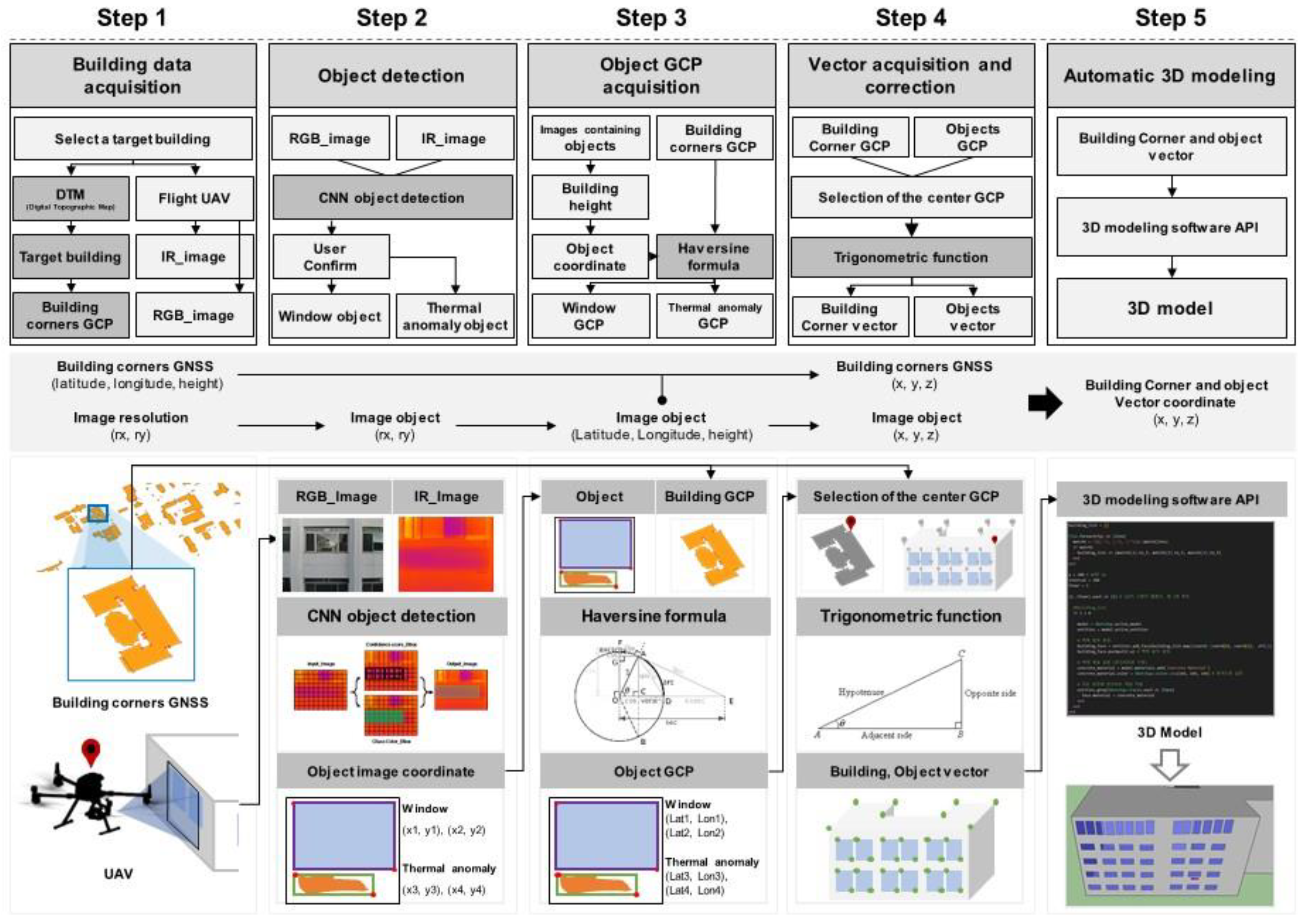
Lastly, the GCP data of the building, as well as the detected window and thermal anomaly objects from the IR and RGB images, were converted into vector coordinates for constructing the 3D model. Finally, SketchUp2023 software was used for model construction. The complete research process is presented in Figure 1.

2.1. Step 1: Building Data Acquisition

Here, building data were collected to enable automated building modeling and thermal anomaly detection. The collected data included RGB and IR images and the GCP information of the building. First, to construct the building’s structural model, GCP coordinates of the target building (containing information about the edges of the building surface) were collected from a digital topographic map (DTM). Next, envelope information was collected using RGB images to model the openings in the building envelope; these images were used to model windows included in the building envelope through an object recognition algorithm. Lastly, IR image data were collected to detect and record the thermal anomalies; these images were also used to model the thermal anomaly regions detected on the building envelope using an object recognition algorithm.

2.2. Step 2: Object Detection

Here, a CNN-based object recognition algorithm was used to detect windows and thermal anomaly regions for modeling from the RGB and IR images collected in Step 1. For window detection, a bounding box (bbox) method was used, considering the typical shape of windows, whereas thermal anomalies (which exhibit irregular forms) were detected using a polygon-based method. To accurately detect objects with different geometric characteristics, this study adopted the YOLOv5 model, which enabled the detection of both bbox-based and polygon-shaped objects [19]. The concept of this model is discussed in Section 2.2.1 and Section 2.2.2. For the recognized window object regions, (x, y) coordinates corresponding to the top-left and bottom-right corners of the bounding box were obtained in image resolution. For thermal anomaly regions, all (x, y) coordinates of the boundary points of the detected polygon-shaped object region were obtained. These coordinates were converted into GCPs and used for modeling window objects and thermal anomaly objects in the building.

2.2.1. You Only Look Once Version 5

The purpose of this algorithm is to identify objects within an image and extract their corresponding coordinates in resolution space. Consequently, YOLOv5—a model capable of performing both bbox-based and polygon-based object detection—was adopted. YOLOv5 has been widely used in various fields owing to its high accuracy and processing speed [20]. It can predict object classes corresponding to bounding boxes and polygons within an input image.

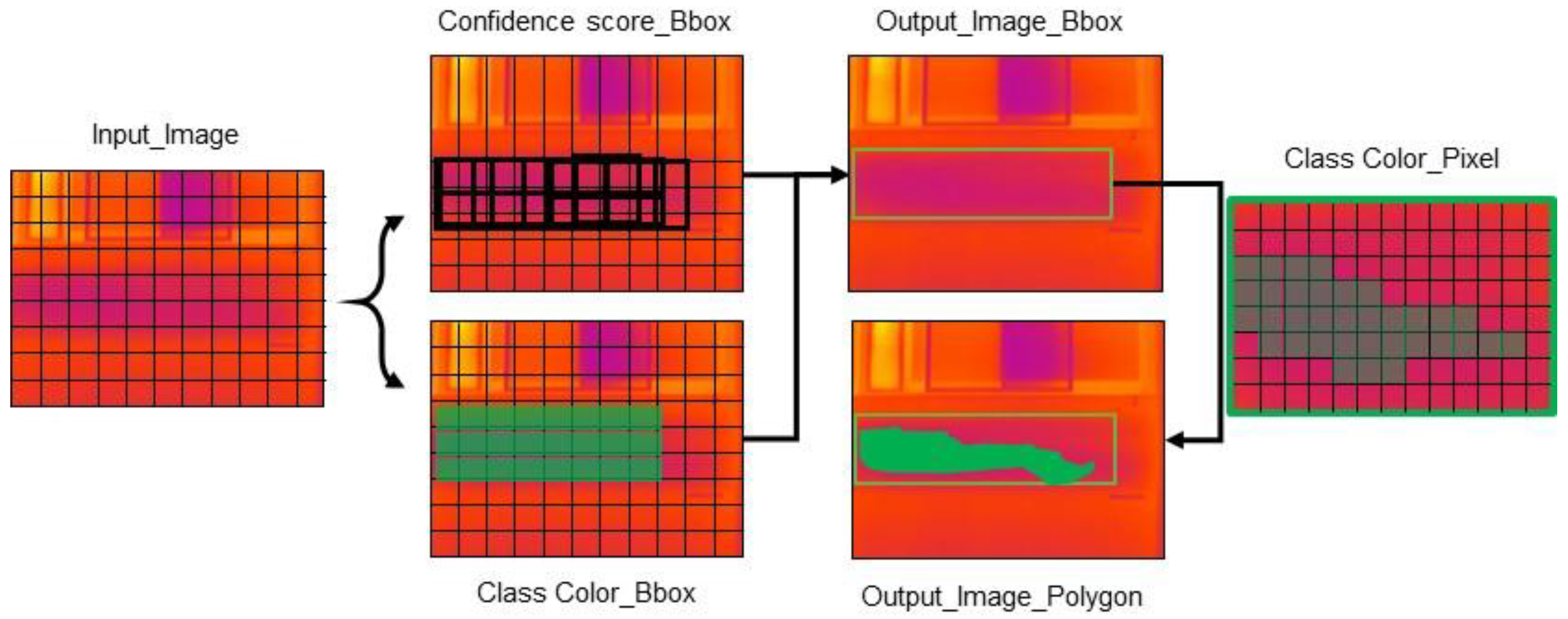
In this study, the input image was first divided into an x × x grid. Then, multiple thin bounding boxes of various sizes were generated within the grid. The algorithm could predict the expected location of the trained object within the bounding box. A confidence score could then be calculated for each predicted location, with the bounding box in these areas becoming thicker. Finally, the thin bounding boxes were removed, leaving only the thick bounding boxes. The non-maximum suppression (NMS) algorithm could then be applied to the remaining bounding boxes to determine the final bounding box selection [21]. In the case of segmentation—which predicts the shape of an object at the location rather than just its location—the pixel attributes could be analyzed within the final predicted bounding box to generate a pixel-wide mask for object separation [22,23]. Figure 2 describes this process.

2.2.2. Object Detection Evaluation Metrics

To assess the reliability of the image object detection model, the average precision (AP) was employed. The AP is a key metric for evaluating object recognition performance; it is derived from the precision–recall (PR) relationship, which is based on the counts of true positives (TPs), false positives (FPs), and false negatives (FNs) calculated by comparing the predicted and ground truth bounding boxes. A critical element in this evaluation is the intersection over union (IoU), which quantifies the overlap between the predicted and actual bounding boxes; a value closer to 1 indicates greater similarity. Alongside AP, additional evaluation metrics such as the F1-score and Dice coefficient were considered to provide a more comprehensive performance analysis. The F1-score, representing the harmonic mean of precision and recall, helps balance the trade-off between these two metrics, particularly in the case of class imbalance. The Dice coefficient, mathematically similar to the F1-score, is widely used in segmentation tasks and places more emphasis on the overlapping region than the IoU. Together, these metrics—AP, IoU, F1-score, and Dice—offer a robust assessment of both detection accuracy and model consistency, with the AP being calculated as the area under the PR curve across various IoU thresholds.

$$IoU={\displaystyle \frac{\left|Prediction \cap Ground Truth\right|}{\left|Prediction \cup Ground Truth\right|}},$$

(1)

$$Dice={\displaystyle \frac{2·\left|Prediction \cap Ground Truth\right|}{\left|Prediction\right|+\left|Ground Truth\right|}},$$

(2)

$$\mathrm{P}\mathrm{r}\mathrm{e}\mathrm{c}\mathrm{i}\mathrm{s}\mathrm{i}\mathrm{o}\mathrm{n}={\displaystyle \frac{TP}{TP+FP}},$$

(3)

$$\mathrm{R}\mathrm{e}\mathrm{c}\mathrm{a}\mathrm{l}\mathrm{l}={\displaystyle \frac{TP}{TP+FN}},$$

(4)

$$\mathrm{A}\mathrm{P}={\sum }_n({recall}_n-{recall}_{n-1}){precision}_n,$$

(5)

$$F1-score={\displaystyle \frac{2·Precision·Recall}{Precision+Recall}}.$$

(6)

2.3. Step 3: Object GCP Acquisition

This section explains the GBP collection method for the objects (windows and thermal anomalies) detected in Section 2.2. First, the resolution coordinates (x, y) of the detected object region can be extracted from the image, along with the camera parameters used for image acquisition (sensor size, focal length, and resolution). The image should also contain GCPs (latitude, longitude, and altitude) recorded at the time of acquisition. Using the GCPs (latitude and longitude) corresponding to the building’s edges and the building height, all relevant GCPs (latitude, longitude, and altitude) corresponding to the building’s surface can be generated.

To link the building’s GCPs with the resolution coordinates of detected objects in the image, the distance between the GCPs in the image and the building’s GCPs can be measured to compute the actual pixel size based on the shooting distance. The Haversine formula can then be used to measure the distance between the two GCPs. This formula calculates the great-circle distance between two points on a sphere (assuming the Earth is a perfect sphere) to determine the distance between them [24,25], and is expressed as follows:

$$\mathrm{a}={sin}^2\left({\displaystyle \frac{\mathsf{\Delta }\varphi }{2}}\right)+cos\left({\varphi }_1\right)·cos\left({\varphi }_2\right)·{sin}^2\left({\displaystyle \frac{\mathsf{\Delta }\lambda }{2}}\right),$$

(7)

$$\mathrm{c}=2·\mathrm{a}\mathrm{t}\mathrm{a}\mathrm{n}2\left(\sqrt{a},\sqrt{1-a}\right),$$

(8)

$$\mathrm{d}=\mathrm{R}·\mathrm{c}.$$

(9)

where Δϕ denotes the difference in latitude between two spherical points; ϕ₁ and ϕ₂ denote the latitudes of point one and point two, respectively; Δλ denotes the difference between the longitudes of the two points; and R denotes the radius of Earth, the average of which is approximately 6371 km.

The distances between all GCPs corresponding to the building area and the image GCPs can be computed, with the shortest distance among them being defined as the camera’s shooting distance. To determine the actual size of the region captured in the image, an RGB image can be processed using a proportional formula that incorporates the photographic metadata (including focal length, sensor size, and resolution) along with the capture distance [17]. For IR images, the actual size can be determined using a formula that considers the metadata (focal length, pixel pitch, and image resolution) and shooting distance [26].

$$\mathrm{R}\mathrm{G}{\mathrm{B}}_{\mathrm{P}\mathrm{I}\mathrm{X}} = {\displaystyle \frac{SS\times L}{R\times FL}},$$

(10)

$${\mathrm{I}\mathrm{R}}_{\mathrm{P}\mathrm{I}\mathrm{X}}=\left({\displaystyle \frac{PP}{FL}}\right)\times L.$$

(11)

Equations (10) and (11) define the actual size corresponding to a single pixel within the image resolution. Here, FL denotes the camera’s focal length, SS denotes the sensor size, L denotes the shooting distance, R denotes the image resolution, and PP denotes the pixel pitch.

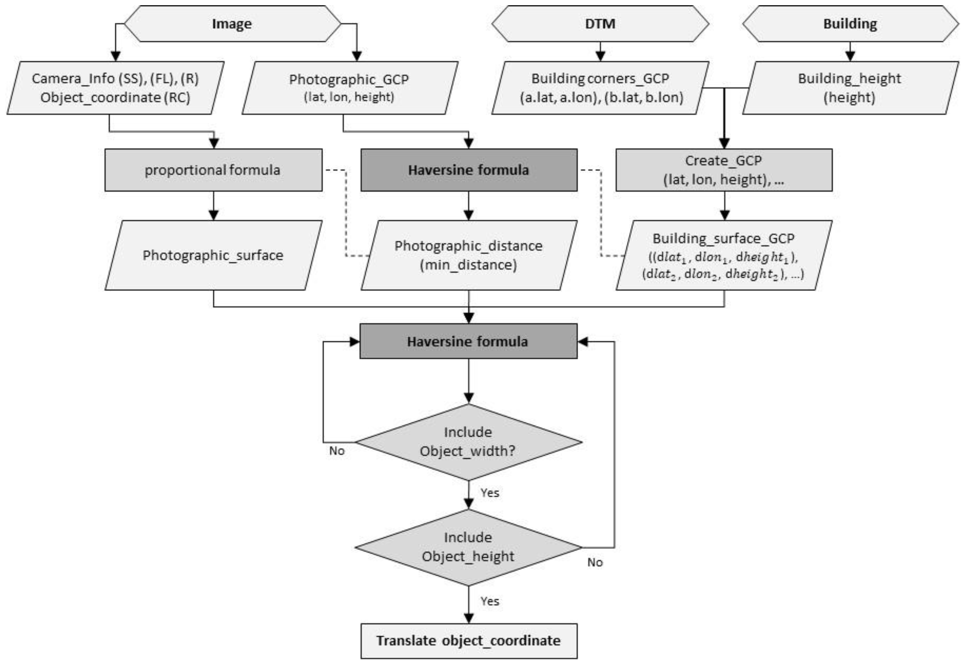
The actual area of the image, calculated using this method, along with the previously obtained image acquisition distance and the GCPs of the building area, can be used to determine the regions of the building in which the detected objects are located. First, the building’s GCP can be defined as 0 based on the central position of the image resolution (x/2, y/2) and the image acquisition distance. Next, the pixel difference between the image’s central coordinate and the detected object’s coordinate (ax, ay) can be computed. The actual distance from the image resolution center to the object position can be determined by multiplying the actual size of a single pixel, obtained from the proportional formula. Here, ax-x represents the horizontal direction of the building, whereas ay-y represents the vertical direction. The measured actual distance value can then be defined as the standard reference for obtaining the object’s GCP. The Haversine formula can be used to compute the distance between the building’s GCP (defined as 0) and the GCP values of other building areas. This process is repeated iteratively until the corresponding GCP is identified for the distances ax-x and ay-y. Once the GCPs for the horizontal and vertical distances are determined, the obtained information can be defined as the GCP of the object’s coordinates. Figure 3 illustrates the process described above.

2.4. Step 4: Vector Acquisition and Correction

In this section, all GCP information (i.e., the building edges and objects) collected in Section 2.3 is vectorized. These vector values serve as coordinate data for constructing the 3D model. For object GCPs, the vector correction algorithm presented in Section 2.4.2 can be used to extract vectors that fall within the range of building corner vector values. The vectors obtained through this process can then be used as positional coordinates for constructing the 3D model.

2.4.1. Vector Acquisition

To obtain the x, y, and z coordinates of the building’s 3D space, one of the acquired GCP values is set as the reference point (0, 0, 0), and the positions of other GCPs are measured accordingly. To define a 3D space, both the distances and directions of other GCPs should be measured relative to the reference point. The Haversine formula, as described in Section 2.3, can be used to calculate the distances. To calculate the directions, a bearing formula based on spherical trigonometry can be applied to determine the azimuth between two points. The distance and direction between the two points can be calculated using the reference GCP and the target GCP. Ultimately, the obtained distance and direction values can then be used to derive 2D vector coordinates (x, y). The z-coordinate, representing the third dimension, is defined as the acquired building height value. The bearing formula can be expressed as in Equation (15) [17,25]:

$$\mathrm{D}\mathrm{L}={{\mathsf{\lambda }}_y-\mathrm{\varnothing }}_{y,}$$

(12)

$$\mathrm{Y}=\mathrm{s}\mathrm{i}\mathrm{n}\left(\mathrm{D}\mathrm{L}\right)\times cos\left({\mathsf{\lambda }}_x\right),$$

(13)

$$\mathrm{X}=\mathrm{c}\mathrm{o}\mathrm{s}\left({\mathrm{\varnothing }}_x\right)\times sin\left({\mathsf{\lambda }}_x\right)-sin\left({\mathrm{\varnothing }}_x\right)\times cos\left({\mathsf{\lambda }}_x\right)\times cos\left(DL\right),$$

(14)

$$\mathrm{B}\mathrm{F}={\displaystyle \frac{\left(atan2\left(Y,X\right)\times \left(\frac{180}{\pi }\right)+360\right)}{360}},$$

(15)

where λ(x, y) denotes the latitude and longitude of the reference point, and ∅(x, y) denotes a value that indicates the latitude and longitude of the relative point.

$$x=\left(d\times \mathit{sin}\left(BF\right)\right),$$

(16)

$$y=(d\times \mathit{cos}\left(BF\right))$$

(17)

where d denotes the Haversine formula-based distance between two points, and BF denotes the bearing-based direction from one point to another.

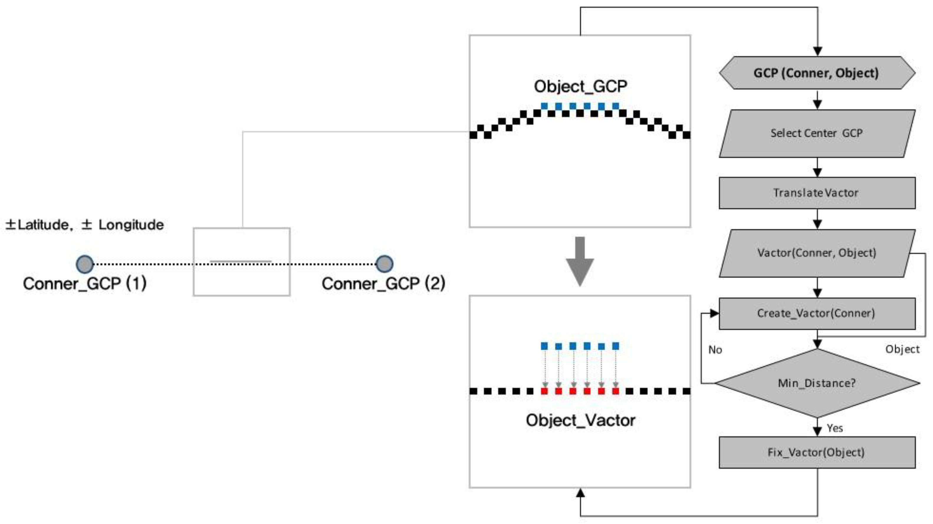
2.4.2. Object GCP-Based Vector Correction

The building shape is based on the Earth’s rotational ellipsoid, and its form consists of curves rather than straight lines. Consequently, in the vector-based 3D model constructed using GCPs corresponding to the building edges, the GCP object locations obtained through the building’s shape can deviate from the vector-based model. To address this, this study employed a vector correction method that replaced the object vector values with the nearest corresponding coordinates within the vector-based 3D model. The vector correction generates virtual point coordinates along a straight line connecting two vector coordinates that define the building edges. The distance between the object vector coordinates and the virtual coordinates can then be iteratively measured. Subsequently, the shortest distance can be determined, and the virtual coordinate at that distance can be defined as the corrected object position. Figure 4 illustrates the structure of the vector correction algorithm.

2.5. Step 5: Vector Coordinate-Based Automatic 3D Modeling

In the final phase of automated 3D modeling utilizing vector coordinates, Ruby code was developed through the SketchUp API to aid seamless tool integration into SketchUp. Using the obtained results, automated 3D modeling was performed by applying geometric tools provided by the SketchUp API [27]. The gathered vector coordinates included unique information such as building contours and object details; thus, vectors corresponding to each distinctive data segment were grouped and treated as individual elements. All vectors constituting window elements were generated using the rectangle tool. Meanwhile, vectors representing thermal anomalies and building contours were created as closed polygons using the line tool. Additional height information was entered for buildings, enabling the construction of a unified building model. Finally, window elements and thermal anomalies were positioned within the building model according to their corresponding locations.

3. Results: Case Study

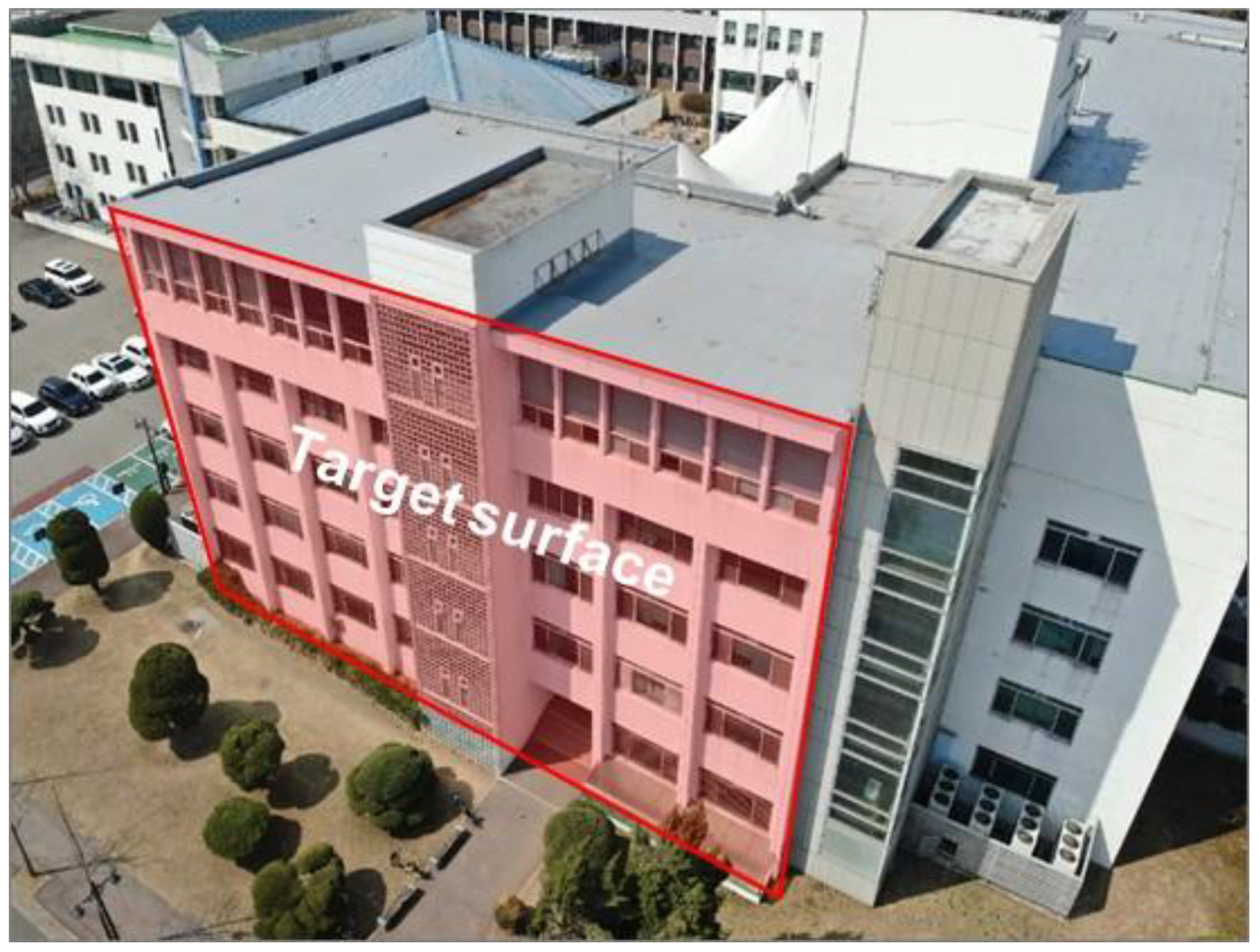
The proposed method was implemented to automatically detect thermal anomaly regions of buildings and record them in the constructed 3D model for management. However, it is essential to comprehensively analyze various factors to identify objects corresponding to thermal anomalies in infrared thermal images, such as structural characteristics, including building columns and beams, and indoor and outdoor environmental conditions. Therefore, in this study, objects corresponding to thermal anomaly areas were defined as insulation areas, trained as objects, and recorded in the three-dimensional model. To validate this method, actual building data were compared with the model data, and errors in the building elements (areas) and thermal anomalies (locations) were analyzed. Additionally, a comparison was made of the number of data points used and the results obtained from the 3D image alignment technique, which were similar to those of previous studies. To apply this research method, an engineering building on a university campus was selected as the study subject. Research involving the target building was conducted after obtaining approval from the appropriate institutional review board. Additionally, to effectively examine the thermal information within the building, one surface capable of indoor temperature regulation was selected for detailed analysis. In the 3D model, the window configuration and the location corresponding to thermal anomalies on this surface were identified, and their similarity to actual locations was evaluated. The exterior of the target building surface is shown in Figure 5.

3.1. Building Data Acquisition

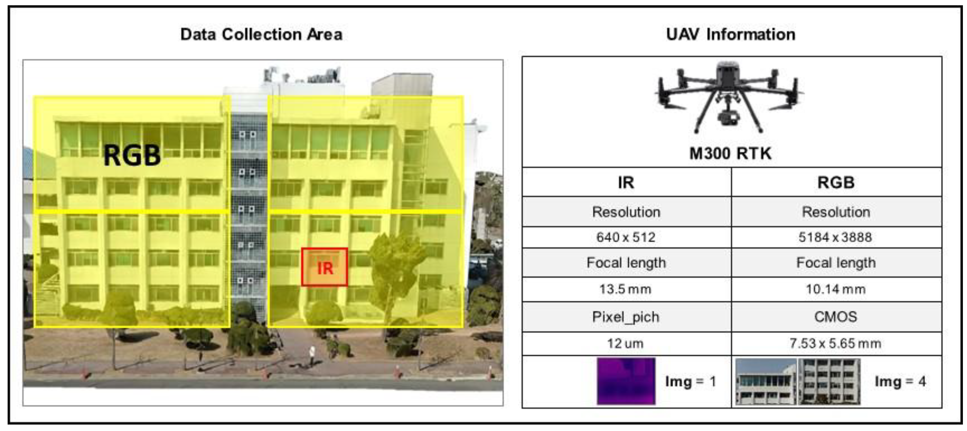
GCPs representing the edge positions for planar modeling were collected from a digital topographic map (DTM) to construct the building envelope of the target building. Additionally, RGB image data capturing the architectural features of windows embedded in the building’s envelope were collected. The image area fully included objects corresponding to windows. Subsequently, IR images were collected to analyze the thermal information of the building envelope. To apply the proposed method, RGB and IR image acquisition were performed with the camera plane aligned horizontally with the target building surface.

The UAV selected for image acquisition was the M300 RTK of DJI Company (Shenzhen, China). It was equipped with real-time kinematic (RTK) functionality to ensure the accurate transmission of GCP data. RTK positioning significantly improves the accuracy of GPS signal collection by applying real-time correction data. This technique is increasingly used in various fields such as geodesy, autonomous navigation, agriculture, and underwater positioning, where precise geolocation is critical [28]. Furthermore, the data acquisition was carried out after obtaining approval for filming, as mandated by national policy guidelines.

The UAV was also equipped with an H20T camera capable of capturing both RGB and IR images, with the resolution of the captured RGB images being 5184 × 3888 pixels. The focal length of the camera lens was set to 10.14 mm, and the sensor used was a 1/1.7-inch complementary metal–oxide–semiconductor (CMOS) sensor. Additionally, the pixel pitch of the IR image was 12 μm, and the focal length was set to 13.5 mm. The data acquired under these conditions are presented in Figure 6.

3.2. Object Detection

To extract resolution coordinates for window and thermal anomaly regions from the acquired images, the YOLOv5 model was trained with 10,000 RGB image-based window bounding box datasets and 880 IR image-based thermal anomaly segmentation datasets.

3.2.1. IR Image

In thermal infrared imagery, the heat distribution of concrete wall surfaces may exhibit varying patterns even on identical facades due to differences in external environmental conditions such as wind, ambient temperature, and humidity, as well as indoor temperature. This study aims to detect thermal anomalies by analyzing deviations in relative temperature distribution patterns, rather than through absolute quantitative thermal measurements.

To facilitate learning of these relative thermal characteristics, a total of 300 thermal images were collected under consistent environmental conditions using the IronRed colormap, which visualizes temperature ranges from −20 °C to 35 °C. In this colormap, higher infrared temperatures are represented as brighter colors, while lower temperatures appear as darker tones. To ensure consistency in thermal distribution across the images, data collection was conducted during the winter season. Moreover, the infrared images were captured from exterior wall surfaces where the difference between indoor and outdoor temperature exceeded 10 °C, enabling clearer detection of radiated heat. Data acquisition was performed just before sunrise to minimize external disturbances such as solar radiation and wind.

To enhance model performance, geometric augmentations including flipping, translation, and rotation were applied to the original dataset, expanding it to a total of 800 training images. The collected dataset included not only concrete wall surfaces but also other architectural components such as columns, openings, and plenum spaces. To isolate the thermal characteristics of the wall itself, non-wall areas were excluded and only the pixel distribution of the wall surface was analyzed.

Based on the extracted color distribution, the wall surfaces were segmented into two groups. Among these, the relatively darker-colored regions were interpreted as areas with superior thermal insulation performance and were consequently defined as thermal anomaly regions for the purpose of this study. These regions were labeled as objects and used as the ground truth data for the segmentation training. Figure 7 presents an example of the thermal images used in the training dataset.

3.2.2. RGB Image

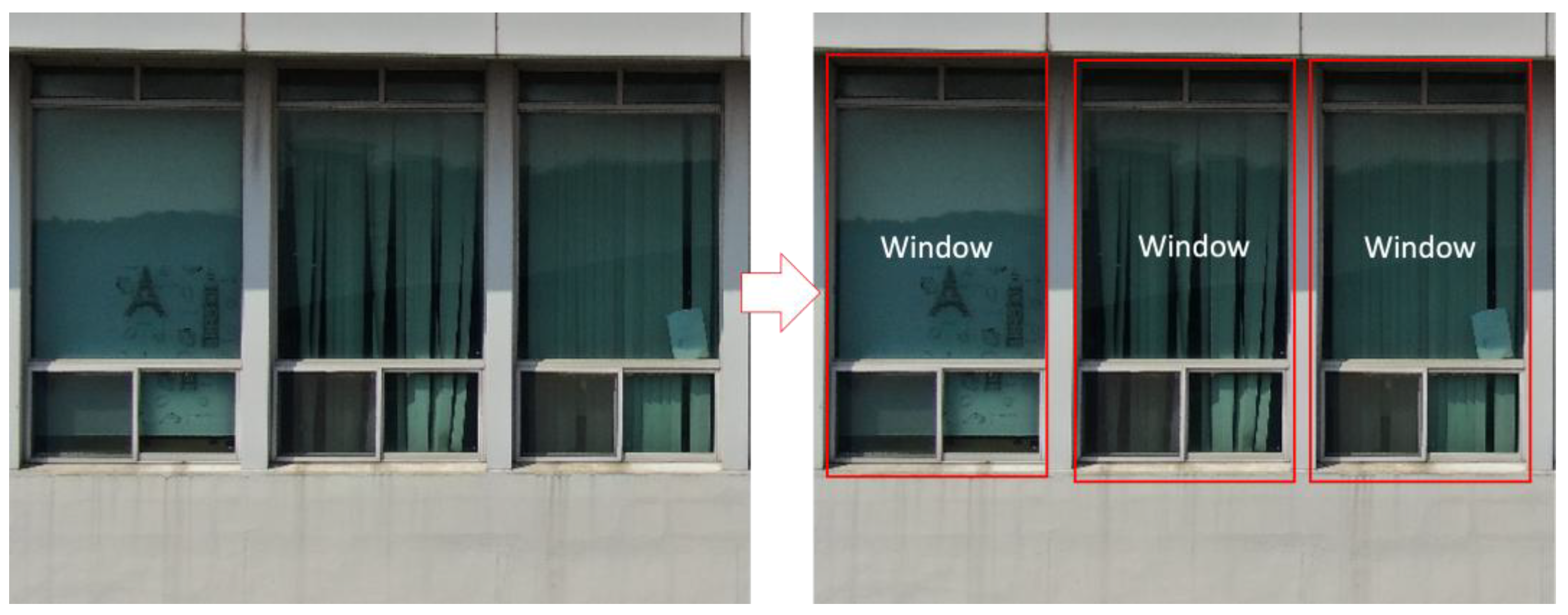
Visible-light images contain data within the spectrum perceivable by the human eye and are used in this study to capture the exterior surfaces of buildings. These images were specifically collected to recognize the shape and identify the location of windows on building facades.

For this purpose, the training dataset was constructed by focusing on windows with a typical rectangular geometry. The window areas were labeled using bounding boxes (bbox), resulting in a total of 10,000 labeled training images.

An example of the images collected under these conditions is presented in Figure 8.

3.2.3. YOLOv5 Model Training

The collected datasets were divided into three subsets—training, validation, and testing—to evaluate the model’s learning capability and overall performance. Selected hyperparameters were adjusted in order to optimize the training process.

Table 1. Structure of training data.

Image	Train	Val	Test	Size
RGB	9000	500	500	640 × 512
IR	700	50	50	640 × 512

summarizes the datasets and the corresponding hyperparameter settings used for training with both RGB and IR images.

For the RGB dataset, 9000 images were used for training, while 500 images each were allocated for validation and testing. In the case of IR images, 700 were used for training, and 50 images each were assigned to the validation and test sets.

Among the hyperparameters listed in

Table 2. Hyperparameters for model training.

Image	lr0	lrf	Momentum	Weight_Decay	Box	Obj
RGB	0.01	0.01	0.937	0.0005	0.05	1.0
IR	0.00967	0.0108	0.97	0.0005	0.0704	1.02

, lr0 is related to the learning convergence speed and training stability. High values of lr0 may lead to instability in segmentation tasks; thus, it was carefully reduced through tuning. The lrf parameter plays a critical role during the fine-tuning phase, while momentum affects both the convergence rate and stability of the training process. The weight_decay parameter contributes to improving the model’s generalization performance and helps prevent overfitting. Lastly, the box and obj parameters influence the accuracy of bounding box predictions and object presence detection, respectively. These influential hyperparameters were selectively adjusted to improve training efficiency. 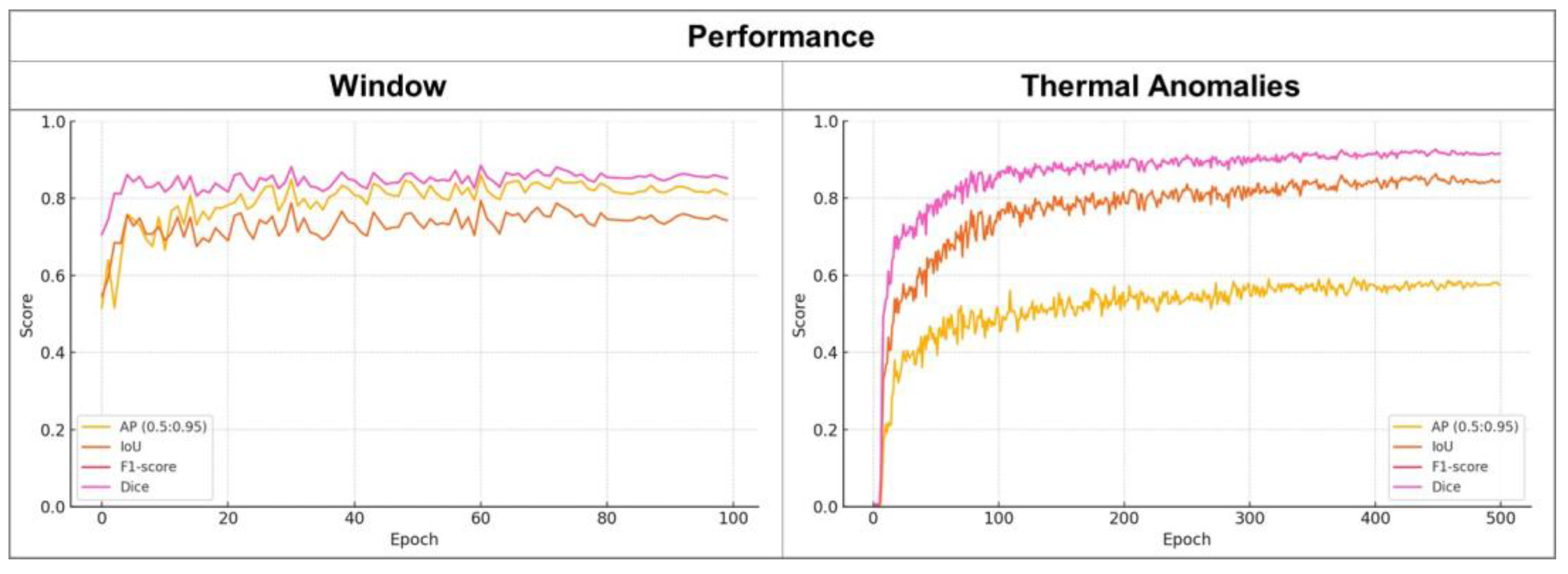The resulting performance of each model after hyperparameter tuning is illustrated in Figure 9.

The window detection model was trained over 100 epochs, and it was observed that the model began to learn the key structural features of windows correctly after approximately 20 epochs. The training and validation curves exhibited a stable pattern, maintaining performance metrics within the range of 0.7 to 0.9. The evaluation results demonstrated high detection performance, with an average precision (AP) of 0.89, an intersection over union (IoU) of 0.74, and both the F1-score and Dice coefficient reaching 0.86.

In the case of the thermal anomaly segmentation model, training was conducted over 500 epochs. The model appeared to have learned the fundamental thermal patterns by around epoch 50, after which a stable convergence trend was observed. The evaluation metrics showed an AP of 0.59, an IoU of 0.84, and both an F1-score and Dice coefficient of 0.91. While the pixel-wise overlap was high, the relatively lower AP in high-score intervals suggests a reduced detection reliability in those regions.

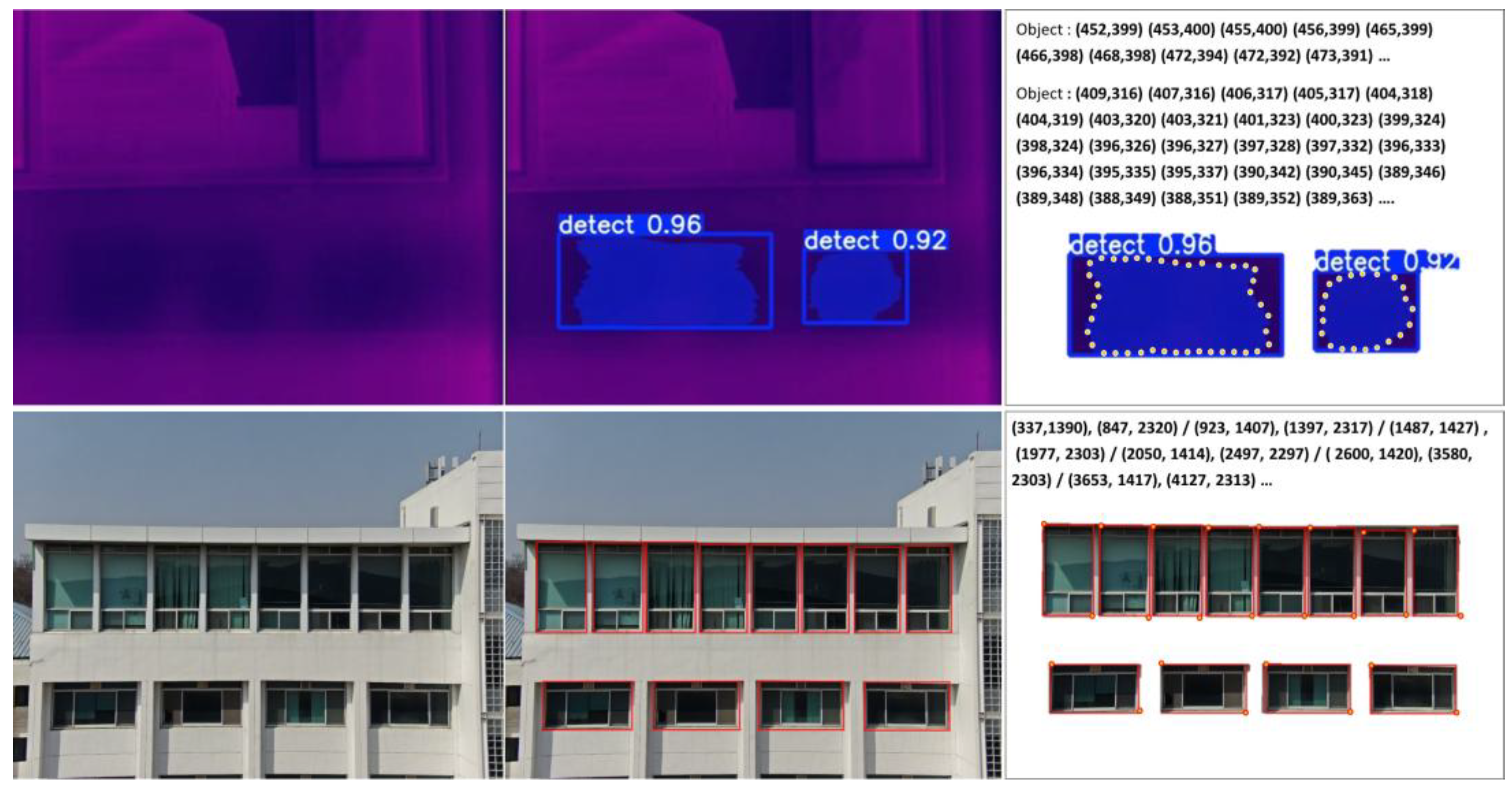
The trained model was used to detect windows in the RGB images as bounding boxes, extracting the resolution coordinates of the top-left and bottom-right corners of each bounding box. Additionally, the IR images were used to obtain resolution coordinates corresponding to the polygon in the thermal anomaly segmentation. The detection results for the windows and thermal anomaly regions, along with their corresponding coordinates, are shown in Figure 10.

3.3. Object GCP Acquisition

The image resolution coordinates of the detected windows and thermal anomaly regions obtained in Section 3.2 were computed as GCPs positioned on the building, using the edge coordinates acquired from the DTM and the building’s height values. First, the GCP_2d points forming the lines between two corner GCP_2ds constituting the outer lines of the building were determined based on the latitude and longitude values (GCP_2d) of the building’s corners. Next, the distances between the collected GCP_2d values from the RGB and IR images and the GCP_2d values forming the building edges were computed using the Haversine formula. The GCP_2d with the shortest distance was then defined as the image acquisition distance.

Next, the height values were added to GCP_2d points along all lines corresponding to the building’s outer edges, defining them as 3D latitude, longitude, and height coordinates. Lastly, by comparing the height values contained within the image, the UAV’s shooting position could be defined within the 3D space. The actual pixel size was calculated based on the defined image acquisition position in the 3D space, the acquisition distance, and the performance of the camera used. This calculation could then be used to measure the building area captured within the image. Finally, the GCPs for the windows and anomaly regions within the acquired area could be defined. The shapes obtained using the GCPs are shown in Figure 11.

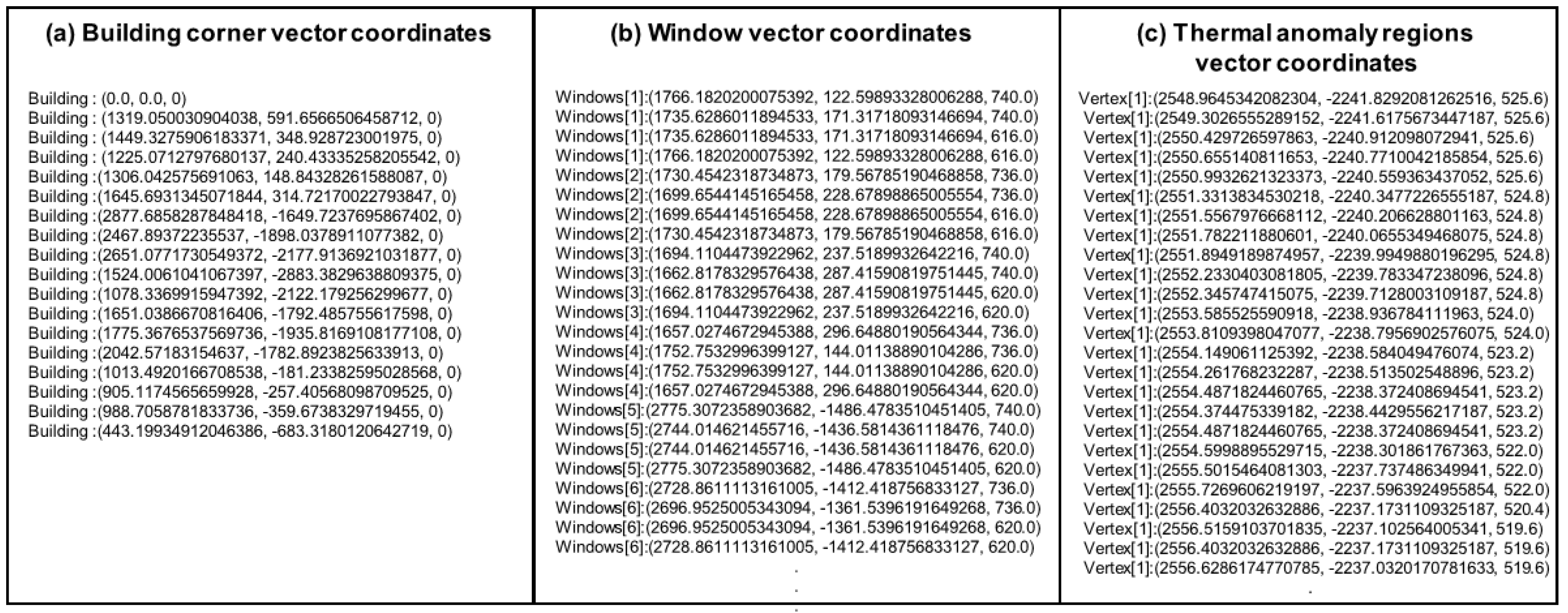
3.4. Vector Acquisition and Correction

One of the previously acquired building corner GCP values was designated as the reference vector coordinate (0, 0, 0). Subsequently, the remaining building corner GCP values were converted into vector coordinates by computing their relative distances from this reference point. The GCP values for the windows and thermal anomaly regions could also be converted into vector coordinates using the same method. The building vector coordinates were then used for refining to obtain the final vector coordinates. The information on the coordinates is shown in Figure 12.

3.5. Automatic 3D Modeling

A 3D model was developed using vector coordinates with modeling tools such as SketchUp. The SketchUp API-based modeling tool (e.g., for creating surfaces, lines, and heights) was used, with the building’s corner vector coordinates first being used to create its shape, after which additional vector coordinates were entered for the windows and thermal anomaly regions on the respective building wall surfaces. This method was developed in Ruby and executed as active code in the SketchUp 2017 application. Figure 13 shows the results of the three-dimensional model.

The actual dimensions of the building were compared with those of the modeled building, the results of which are presented in

Table 3. Comparison of object measurements.

Object	Real Data (m)	Modeling Result (m)	Deviation (%)
Building	80.0 × 45.0 × 21.0	79.5 × 45.3 × 21.3	1.47
Window 1	3.10 × 1.68	3.08 × 1.63	3.62
Window 2	1.55 × 3.70	1.59 × 3.15	17.45

.

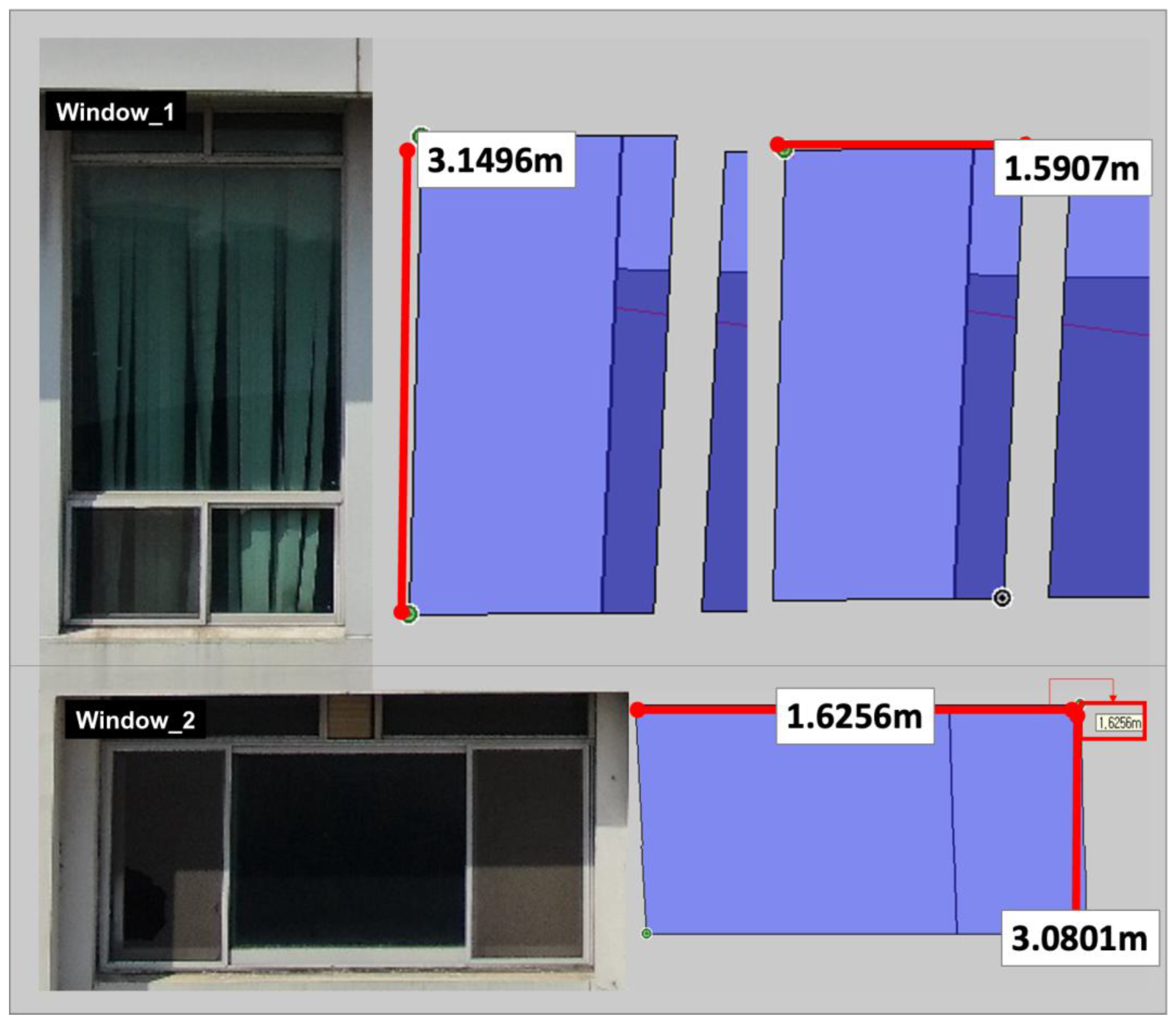
A comparison of the overall building dimensions and the dimensions of the input windows showed errors of 1.47% for the building, 3.62% for Window 1, and 17.45% for Window 2. Additionally, the front facade of the building exhibited a high degree of consistency. The thermal anomaly regions were examined based on the window positions, and all entered thermal anomalies were confirmed to be consistent with the visually identified locations. Furthermore, the shapes of the thermal anomaly regions were confirmed to be structurally similar. Figure 14 shows the actual shape of the window and the window representation generated in the 3D model.

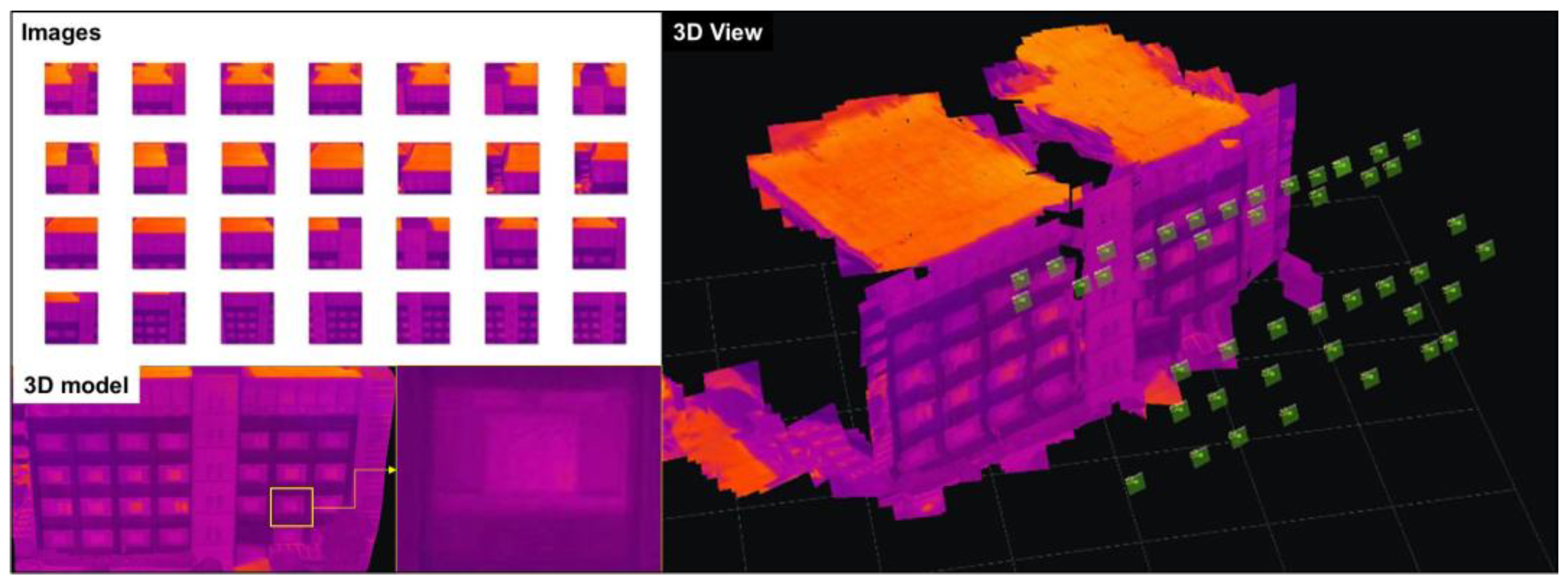
Next, a 3D image matching model based on a previous study was also constructed to evaluate the efficiency of the 3D model constructed using the proposed research method. A total of 44 thermal images were acquired of the same wall surface for comparison of shapes, the number of images used, and data size. ContextCapture software [29] was used for image alignment. The configuration of the image data used for modeling and the resulting outputs from both the proposed and the previous methods are shown in Figure 15.

Although the 3D image alignment model requires a larger number of image datasets compared to the SketchUp-based shape constructed using the proposed method, it provides a more intuitive representation of building features by closely resembling the actual geometry. Additionally, thermal images have lower resolution than visible-light images, resulting in smaller data sizes per image. However, due to this lower resolution, each pixel covers a wider temperature range, which can lead to alignment quality issues, as seen in the yellow areas in Figure 15. To overcome such resolution limitations, image data should be collected from closer distances, and a higher number of overlapping images is required to ensure proper alignment.

In contrast, the 3D model proposed in this study identifies window areas that indicate the spatial characteristics of the building using only four images and reconstructs the building shape in 3D. Moreover, thermal image data are used specifically to identify thermal insulation areas on the exterior wall, allowing for targeted data acquisition with a single image per location to identify insulation-related features and generate the corresponding 3D model.

Table 4. Comparison of the images and model data used.

Data	3D Image Matching	Proposed Method-Based 3D Model
Images	44	4
Image size	35.9 MB	28.3 MB
Model size	2.36 MB	0.088 MB

summarizes the image types, data sizes, and specific features captured through each dataset.

4. Discussion

The proposed methodology demonstrated its ability to model the target building. Even in the absence of architectural drawing data, it enabled the 3D modeling of high-rise buildings with limited accessibility using UAVs, allowing for a relatively fast generation of a structurally similar building model. The identified thermal anomaly regions in the 3D model were consistent with actual locations in the building, confirming that they could be identified using the 3D model. The findings of this study indicate that the proposed method could enable the identification of thermal anomaly regions and facilitate faster and more efficient documentation and management of these regions during inspections. However, several limitations exist.

The thermal insulation object detection model employed in this study was trained on winter-season infrared images of flat concrete exterior walls and demonstrated effective performance under these conditions. However, building facades in real-world scenarios may consist of diverse materials beyond concrete, and infrared emission patterns from wall surfaces can vary depending on seasonal conditions. Moreover, not all buildings feature flat geometries; some incorporate curved or irregularly shaped walls. Therefore, future studies should consider the development of diverse training datasets and models tailored for non-planar and irregular building types to evaluate the model’s generalizability across various wall structures and seasons.

The image data used in this study were collected from a single building, and the size of the detected objects in the images closely matched their actual physical dimensions. Nonetheless, discrepancies in object size may arise due to various factors, including coordinate transformation errors and geometric distortions caused by lens characteristics. To improve the accuracy of object dimension estimation, further research is required on correcting image distortion and refining coordinate transformation processes.

This study demonstrated a method for detecting thermal anomaly regions—defined as insulation zones—and recording them within a 3D model. The approach was shown to be an efficient means of documenting and managing the thermal performance of building envelopes. However, converting the color distributions obtained from thermal infrared images into quantifiable temperature values also plays a critical role in thermal performance assessment and long-term insulation management. Quantitative analysis of thermal accuracy in infrared imagery requires not only controlled acquisition conditions—as implemented in this study, including the absence of direct sunlight, minimal wind influence, sufficient difference between indoor and outdoor temperature, and seasonal considerations—but also building-specific structural factors and additional environmental variables. Such analysis demands a higher level of domain-specific expertise and methodological precision. Therefore, future studies should incorporate professional thermographic evaluation techniques to quantitatively assess thermal performance from infrared imagery. This would allow for the classification and segmentation of well-insulated, non-insulated, and degraded insulation areas, enabling their accurate representation in 3D models for more comprehensive and precise insulation management.

Finally, the proposed method was able to generate a 3D model of the building envelope, containing only information related to the exterior structure. For this model to be integrated into a BIM system, it should also incorporate information regarding the internal structure and material composition of the building.

By addressing these limitations, it should be possible to conduct building maintenance more effectively, reducing human risk, minimizing inspection time, and enabling quantitative building performance assessments through simulation-based objective evaluations.

5. Conclusions

This study developed a method for documenting thermal anomaly regions through the automatic modeling of buildings. Initially, the coordinates of building edges were collected using a DTM (Digital Terrain Model), and images of building shapes and heights were acquired through UAV flights. These collected building edge coordinates and height data were then converted into vector coordinates to construct a 3D shape. Subsequently, window structures and thermal anomaly regions within the building images were identified using YOLO-based image object detection, collecting image resolution coordinates for these two types of structures. The collected image resolution coordinates were then converted into vector coordinates corresponding to their 3D shapes by integrating GNSS coordinates embedded in the images. Consequently, the method successfully automated the construction of 3D models utilizing all collected vector coordinates and documented the identified windows and thermal anomaly regions.

Unlike conventional methods that process and construct 3D models of all regions within an image, this approach selectively identifies relevant areas, enhancing documentation and management efficiency. Furthermore, constructing a 3D model based on vector coordinates using dedicated 3D modeling software can provide foundational data for extending the model into a building information modeling (BIM) environment. BIM not only encompasses the building envelope but also integrates comprehensive information on materials, structural elements, and interior spaces. Although this study focused on representing the external geometry of the building, the proposed method ensures scalability to incorporate additional data necessary for full BIM implementation in future research.

By addressing the limitations discussed in Section 4, a maintenance process could be developed to record and analyze thermal anomaly regions in high-rise buildings using the generated building models, enabling more efficient management. The proposed process is expected to reduce the time and cost required for external building inspections while simultaneously ensuring inspector safety during maintenance procedures.