Research on Denoising of Bridge Dynamic Load Signal Based on Hippopotamus Optimization Algorithm–Variational Mode Decomposition–Singular Spectrum Analysis Method

Abstract

Bridge dynamic load test signals are readily contaminated by environmental noise. This reduces the accuracy of bridge structure state assessment. To address this issue, this research proposes a denoising method that combines the hippopotamus optimization algorithm (HOA), variational mode decomposition (VMD), and singular spectrum analysis (SSA). The methodology follows three key phases: First, the HOA optimizes the critical parameters of VMD. Then, the optimized VMD decomposes raw signals into several intrinsic mode components (IMFs). The IMFs below the threshold are removed by calculating the correlation coefficient between each IMF and the original signal. Finally, SSA is introduced for secondary denoising, which helps reorganize bridge signals and eliminate local low-frequency oscillations. The simulation results show that compared with other methods, the root mean square error (RMSE), signal-to-noise ratio (SNR), mean square error (MSE), and mean absolute error (MAE) of the denoised signals achieve on average 16.22% reduction, 2.51% improvement, 62.02% diminution, and 43.74% decrease, respectively, across varying noise levels. Practical validation reveals superior performance metrics: a mean 12.81% lower normalization Shannon entropy ratio (NSER) and a mean 8.44% higher noise suppression ratio (NSR) compared to other techniques. This comprehensive approach effectively addresses noise components in bridge dynamic load test signals.

1. Introduction

The detection and evaluation of bridge safety performance represent a critical task in modern transportation infrastructure management. As an essential part for bridge safety verification, bridge dynamic load testing precisely assesses the bridge structure’s dynamic response through controlled traffic load simulation [1]. The dynamic load test examines how bridges behave under dynamic loads, covering aspects like vibration traits, impact reactions, and fatigue harm [2]. However, bridge dynamic test instruments are currently weak equipment that can be easily disturbed by factors such as geomagnetic fields and space electromagnetic waves. These interference sources introduce substantial noise contamination in acquired dynamic signals, significantly compromising the fidelity of structural condition assessments [3]. Therefore, it is urgent to develop a systematic and robust signal denoising algorithm to guarantee accurate and reliable data in bridge dynamic load tests.

In bridge engineering, various denoising techniques based on structural vibration signals have been widely adopted and implemented. Kordestani et al. [4] developed a novel trendline-based decomposition algorithm where bridge response signals are partitioned through Savitzky–Golay filtering. The removal of noise is accompanied by the storage of noise and higher-order modal vibrations in separate residual signals, facilitating subsequent signal reconstruction and damage localization. Liu et al. [5] pioneered a hybrid denoising architecture integrating ground-based synthetic aperture radar (GBSAR) with second-order blind identification (SOBI). Their methodology exploits GBSAR’s millimeter-scale displacement resolution alongside SOBI’s statistical independence criteria to disentangle noise from bridge deflection dynamics. Fang et al. [6] formulated an improved empirical wavelet transform (EWT) framework for global navigation satellite system (GNSS) data denoising. Their adaptive spectral segmentation mechanism, governed by local maxima detection in Fourier spectra, achieves precise extraction of low-order bridge modes during operational vibrations. Notably, adaptive mode decomposition remains a cornerstone in this field. Empirical mode decomposition (EMD) and ensemble empirical mode decomposition (EEMD) represent prominent adaptive signal processing approaches. EMD is a time–frequency localization analysis method; it decomposes non-stationary signals into a series of intrinsic mode functions (IMFs) [7]. Notably, each IMF represents the intrinsic vibration mode of different frequency components in the signal [8]. By selectively combining these IMFs, the denoised signal sequence can be reconstructed. However, EMD may encounter modal aliasing when processing signals with similar frequency components. To overcome this constraint, EEMD has been proposed [9]. By adding white Gaussian noise to raw signals to enhance decomposition performance of EMD, it helps eliminate the phenomenon of modal aliasing effectively and improve the robustness of the algorithm. Nevertheless, the artificial noise introduced in EEMD may have an impact on the noise components in the original signal, resulting in distortion of the analysis results and loss of feature information.

To address the inherent limitations existing in EMD and its improved version EEMD, variational mode decomposition (VMD) was developed as an innovative alternative [10]. VMD introduces a regularization term to limit the bandwidth of each modal function, reduce spectrum overlap, and effectively suppress modal aliasing. When implementing VMD for bridge feature extraction, it is necessary to set decomposition scales and penalty factors. Current methodologies frequently integrate meta-heuristic optimization techniques to optimize these parameter combinations [11,12,13]. Notably, Nassef et al. [14] proposed an improved VMD based on sailfish optimization (SFO) to identify the fault in rolling bearings, which significantly improved the accuracy in extracting fault features and exclusion of noise effect. However, the global search ability and algorithm convergence speed of SFO in dealing with complex problems need to be strengthened. Zhang et al. [15] investigated a hybrid approach combining the grasshopper optimization algorithm (GOA) with VMD for mechanical vibration signal denoising. This method uses the weighted kurtosis index as the index to screen the modes and improve the denoising accuracy. However, GOA faces the challenges of local optimization and convergence speed. According to the shortcomings of the existing algorithms, Amiri et al. [16] introduced the hippopotamus optimization algorithm (HOA). As a new population-based optimization method, it achieved a superior balance between global exploration and local exploration. This innovative optimizer effectively circumvents premature convergence while maintaining rapid convergence characteristics [17]. Recent applications demonstrate the practical efficacy of HOA-VMD integration, as evidenced by Chen et al. [18], who successfully applied this combination to reduce the error of synchronous oscillation mode identification. The results verified the excellent optimization ability of the HOA and the effectiveness and accuracy of the HOA-VMD.

In addition to parameter setting, VMD finds difficulty in dealing with the instantaneously changing frequency components during the processing of non-stationary bridge signals. As a result, the denoised signal has local low-frequency oscillation, which becomes a non-negligible signal error. To make up for the deficiency of VMD, prior studies [19,20] combined wavelet threshold with VMD for acoustic and ultrasound signal denoising. The results show that this method can significantly reduce the error of reconstructed signals. However, this hybrid method exhibits limited effectiveness for bridge signal processing, as the wavelet threshold technique inadequately suppresses white noise components in bridge signals. Further evidence of VMD’s limitations emerges. Zhou et al. [21] used VMD to remove the noise to suppress the seismic noise. Because of the residual low-frequency noise, there were obvious oscillations in the denoised signal. Remarkably, the subsequent application of singular spectrum analysis (SSA) for secondary denoising achieved great oscillation suppression. This highlights SSA’s potential as an effective complement to VMD-based approaches, especially for processing signals with large amplitude changes, which can effectively reduce the low-frequency oscillation after denoising.

Aiming at the noise interference phenomenon in bridge dynamic load test signals, this research proposes a hybrid denoising method that integrates HOA to adaptively optimize VMD parameters, enabling VMD to decompose raw signals into IMFs. Finally, we introduce SSA to eliminate oscillatory components and reconstruct the denoised signal while preserving critical structural response characteristics.

The sequence of this paper is organized as follows: The system of bridge dynamic load test signal denoising is presented in Section 2. A theoretical background on VMD, HOA, and SSA is introduced in Section 3. Section 4 is a simulation to verify the feasibility of the denoising method in this paper. To verify the practicability of the method, Section 5 shows the experiment process and results. Finally, discussion and conclusions are presented in Section 6 and Section 7, respectively.

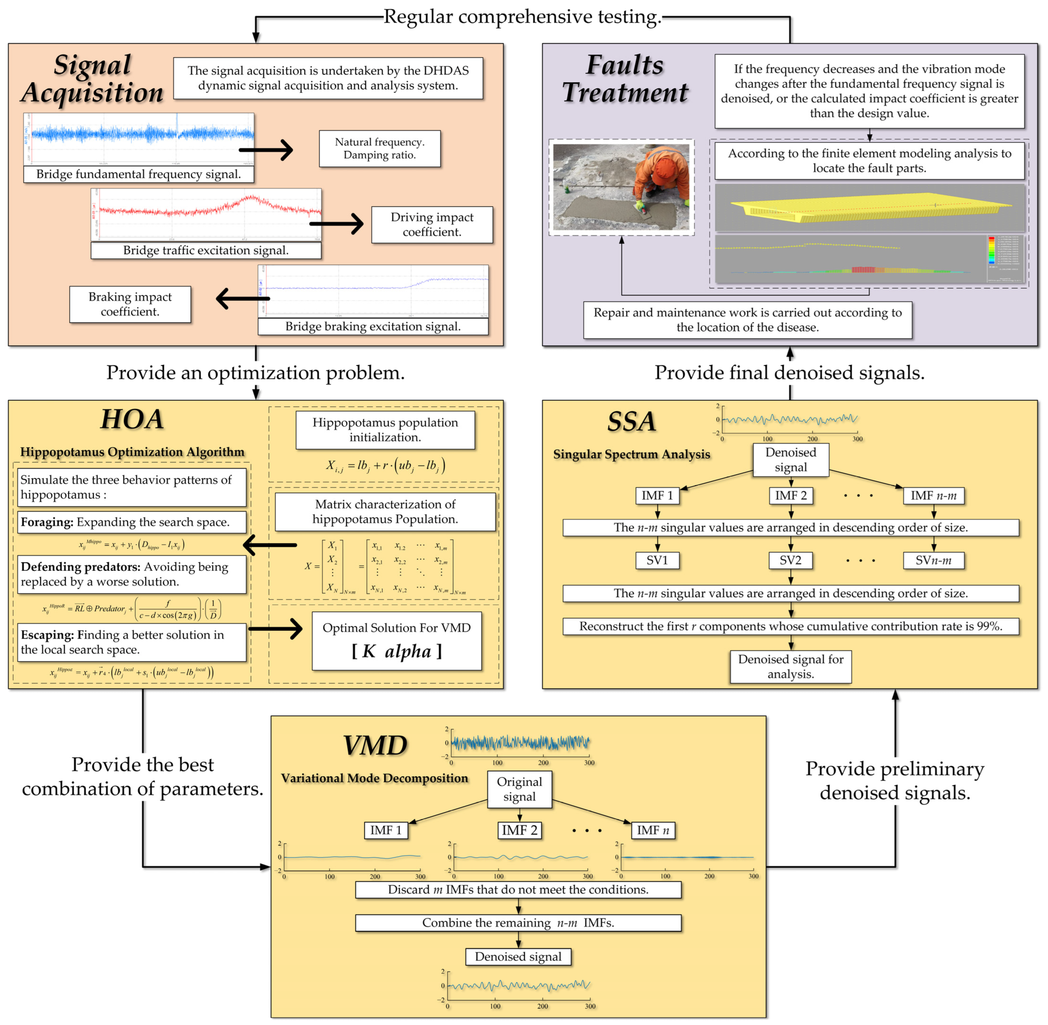
2. System Framework

This research proposes a system framework of signal denoising algorithm for bridge dynamic load test, with particular emphasis on developing an advanced denoising solution to address signal quality challenges in structural health monitoring. As depicted in Figure 1, the DHDAS dynamic signal acquisition and analysis system is used to collect and analyze the dynamic load test signals of the bridge. The denoising module constitutes the primary contribution of this research, which utilizes HOA, VMD, and SSA as the core innovation. This tripartite algorithmic combination effectively eliminates noise components from raw bridge dynamic load test signals while preserving critical structural vibration characteristics.

To demonstrate the engineering applicability, denoised signals undergo validation through performance index calculations referenced in technical specifications. If the signal’s characteristics are abnormal or the calculated impact coefficients are greater than the design value, the reasons are further analyzed by using finite element analysis. Afterwards, the structural faulty areas are accurately located, thereby providing a scientific basis for the subsequent maintenance and repair of the bridge structure.

3. Methodology

In this research, the VMD parameters are optimized through the HOA to enhance signal processing performance. Then, the raw bridge dynamic load test signal is decomposed into a series of IMFs using the optimized VMD. To deal with residual low-frequency interference, SSA is introduced to eliminate the low frequency oscillation in the signals after preliminary processing by VMD. Finally, the denoised signal is obtained by reconstructing through superposition of the optimized IMF components. The denoising process is depicted in Figure 2.

3.1. Variational Mode Decomposition

Bridge dynamic load test signals exhibit nonlinear and non-stationary characteristics, manifesting as time-dependent statistical properties, including instantaneous mean and variance. To mitigate these signal characteristics, VMD employs simultaneous estimation of modes with different center frequencies through non-recursive mode decomposition. By effectively extracting the periodic and transient characteristics of signals, VMD decomposes raw signals into a series of IMFs with specific center frequencies and narrow band characteristics [22,23,24].

The given bridge dynamic load test signal is decomposed into multiple AM-FM signals, denoted as

$$u_i\left(t\right)=A_i\left(t\right)\cos [\varphi \left(t\right)]$$

(1)

where $A_i\left(t\right)$ is the amplitude of IMF; $\varphi \left(t\right)$ is the phase function of IMF.

Based on this, the optimization problem of VMD can be expressed as a constrained variational problem:

$$\underset{\left\{u_i\right\},\left\{{\omega }_i\right\}}{\min }\left\{{\displaystyle \sum _{i=1}^K{‖{\partial }_t\left[\delta \left(t\right)+\frac{j}{\pi t}{u}_i\left(t\right)\right]e^{-j{\omega }_{i}t}‖}_2^2}\right\},s.t.{\displaystyle \sum _{i=1}^K{u}_i\left(t\right)=f\left(t\right)}$$

(2)

where $\left\{u_i\right\}=\left\{u_1,\dots ,u_k\right\}$, $\left\{{\omega }_i\right\}=\left\{{\omega }_1,\dots ,{\omega }_k\right\}$, $K$ is the number of intrinsic mode components, $s.t.$ denotes the constraint condition, $u_i\left(t\right)$ is the modal function of signal $f\left(t\right)$, $\delta \left(t\right)$ denotes the Dirac distribution, $j$ represents the signal sequence, ${\omega }_i$ is the center frequency of each modal component, and $i$ is the number of iterations.

The quadratic penalty factor $\alpha$ is introduced to suppress the Gaussian noise in the bridge dynamic load test signal. By using the Lagrange operator to maintain the tightness of the constraint, transform Equation (2) into an unconstrained variational problem. The augmented Lagrange expression is obtained as

$$L(\left\{u_i\right\},\left\{{\omega }_i\right\},\lambda )=\alpha {\displaystyle \sum _{i=1}^K{‖{\partial }_t\left[\left(\delta \left(t\right)+\frac{j}{\pi t}\right)u_i\left(t\right)\right]e^{-j{\omega }_{i}t}‖}_2^2+}{‖f\left(t\right)-{\displaystyle \sum _{i=1}^K{u}_i\left(t\right)}‖}_2^2+〈\lambda \left(t\right),f\left(t\right)-{\displaystyle \sum _{i=1}^K{u}_i\left(t\right)}〉$$

(3)

where $L\left(·\right)$ is the Lagrange function; $\lambda$ is the Lagrange multiplier term. Use the alternating direction multiplier combined with the Fourier transform iterative algorithm to obtain the optimal solution of Equation (3). Iterate the current solution until Equation (4) is satisfied, and output $K$ modal components:

$${\displaystyle \sum _{i=1}^k\frac{{‖{\widehat{u}}_i^{n+1}-{\widehat{u}}_i^n‖}_2^2}{{‖{\widehat{u}}_i^n‖}_2^2}}<\epsilon$$

(4)

where $n$ is the number of iterations, ${\widehat{u}}_i^{n+1}$ is the Fourier transform of $u_i^{n+1}$, and $\epsilon$ represents the allowable error, usually with a value of $1\times {10}^{-7}$.

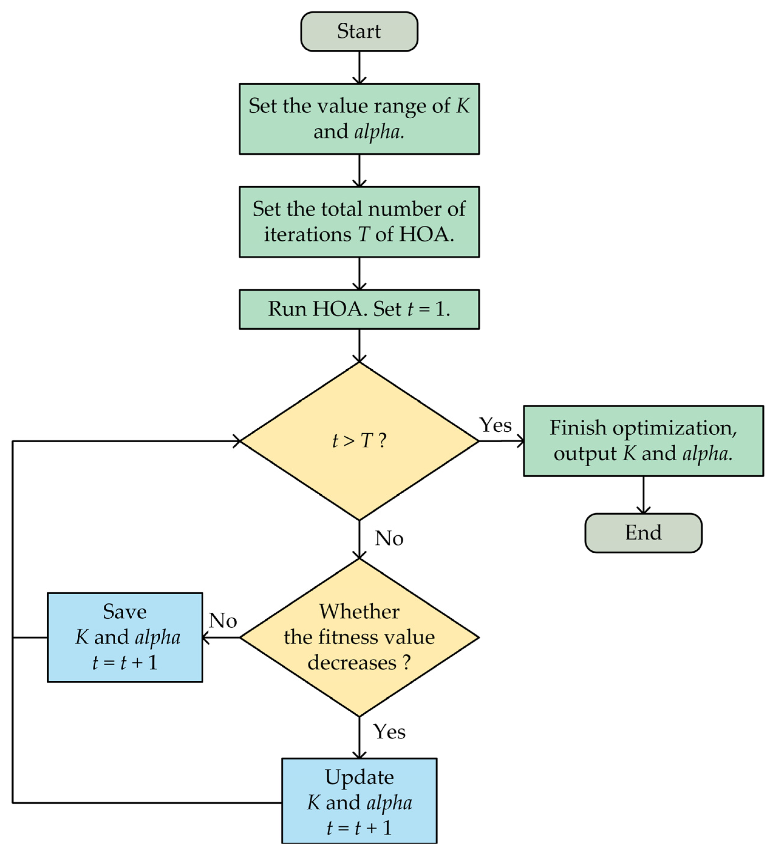
3.2. Hippopotamus Optimization Algorithm

During the bridge dynamic load test analysis, the denoising performance of VMD is critically influenced by two key parameters: decomposition scale ($K$) and penalty factor ($\alpha$). Current parameter determination approaches can be categorized into three primary methodologies: The first relies on empirical selection based on engineering experience, which can easily lead to inadequate signal decomposition because of a lack of adaptability [25]. The second employs self-adaptive VMD. However, it is difficult to always meet the iterative conditions [26]. The third category utilizes metaheuristic optimization algorithms such as WOA, GWO, and others. Although these algorithms can optimize VMD parameters, there are significant performance variations between efficiency and accuracy due to the different core links such as algorithm search space construction, iterative solution process, parameter dynamic update, solution evaluation, and screening [27]. To tackle these limitations, Amiri et al. proposed the HOA recently. It demonstrates superior convergence characteristics and robustness across multiple benchmark functions compared to conventional optimization techniques. Therefore, this research introduces HOA as an innovative approach for VMD parameter optimization. Aiming to enhance its noise denoising capabilities for dynamic load test signals of bridge. The systematic workflow for HOA-based VMD parameter optimization is illustrated in Figure 3.

The pseudo-code of the HOA is shown in Algorithm 1. According to the initialized hippopotamus population, each hippopotamus is represented by a single vector. The hippopotamus population matrix is characterized as

$$x_{i,j}=l{b}_j+r·\left(u{b}_j-l{b}_j\right)$$

(5)

$$X={\left[\begin{array}{c}{X}_1\\ X_2\\ ⋮\\ X_N\end{array}\right]}_{N\times m}={\left[\begin{array}{cccc}{x}_{1,1}& x_{1.2}& \cdots & x_{1,m}\\ x_{2,1}& x_{2,2}& \cdots & x_{2,m}\\ ⋮& ⋮& \ddots & ⋮\\ x_{N,1}& x_{N,2}& \cdots & x_{N,m}\end{array}\right]}_{N\times m}$$

(6)

where $X$ denotes the position of the candidate solution; $r$ is a random number between 0 and 1; $lb$ and $ub$, respectively, represent the lower and upper boundaries of decision variables; $N$ represents the population size of the hippos in the population; $m$ represents the number of decision variables in the problem, $i=1,2,\dots ,N$, $j=1,2,\dots ,m$.

• Phase 1: Renewal of the hippopotamus’ position in a river or pond (Exploration)

According to the position of the leading hippopotamus, the group members update their positions in the place of residence. The algorithm is expressed as expanding the search space:

$${x_{ij}}^{Mhippo}=x_{ij}+y_1·\left(D_{hippo}-I_1{x}_{ij}\right)$$

(7)

As the number of iterations increases, juvenile hippopotamuses, driven by curiosity, increasingly depart from the group to explore the surrounding environment:

$${x_{ij}}^{FBhippo}=x_{ij}+h_1·\left(D_{hippo}-I_{2}M{G}_i\right)$$

(8)

where ${x_{ij}}^{Mhippo}$ denotes the location of the male hippopotamus, $D_{hippo}$ denotes the position of the dominant hippopotamus, $y_1$ is a random number, $M{G}_i$ is the average value of random hippopotamuses, $h_1$ is a random number or vector, $I_1$ and $I_2$ are integers between 1 and 2, $i=1,2,\dots ,N/2$, and $j=1,2,\dots ,m$.

• Phase 2: Hippopotamus defense against predators (Exploration)

Update the position of predators and simulate the random walk of them according to the Levy flight vector. When the fitness value of the hippopotamus is greater than the fitness value of predators, the hippopotamus defends the predators according to Equation (9).

$${x_{ij}}^{HippoR}=\overrightarrow{RL}\oplus Predato{r}_j+\left({\displaystyle \frac{f}{c-d\times \cos \left(2\pi g\right)}}\right)·\left({\displaystyle \frac{1}{\overrightarrow{D}}}\right)$$

(9)

Otherwise, the hippopotamus escapes from the predators according to Equation (10). It is reflected in the algorithm as a fine-tuning of the current solution to avoid being replaced by a worse solution:

$${x_{ij}}^{HippoR}=\overrightarrow{RL}\oplus Predato{r}_j+\left({\displaystyle \frac{f}{c-d\times \cos \left(2\pi g\right)}}\right)·\left({\displaystyle \frac{1}{2\times \overrightarrow{D}+{\overrightarrow{r}}_3}}\right)$$

(10)

where $Predato{r}_j$ represents the position of the predator in the dimension $j$; $\overrightarrow{RL}$ is a random vector with levy distribution; ${x_{ij}}^{HippoR}$ is the position of the hippopotamus relative to the predator; $\overrightarrow{D}$ is the distance between the hippopotamus and the predator; $c$, $d$, $f$, and $g$ are random numbers; ${\overrightarrow{r}}_3$ is a random matrix of dimension; $i=1,2,\dots ,N$; and $j=1,2,\dots ,m$.

• Phase 3: Hippopotamus escapes from predators (Exploitation)

By simulating the behavior of the hippopotamus escaping from the predator and attempting to move to a safer position, the algorithm is further refined to find a more optimal solution in the local search space:

$${x_{ij}}^{Hippo\epsilon }=x_{ij}+{\overrightarrow{r}}_4·\left({{lb}_j}^{local}+s_1·\left({{ub}_j}^{local}-{{lb}_j}^{local}\right)\right)$$

(11)

where ${x_{ij}}^{Hippo\epsilon }$ is the nearest safe location; $s_1$ is a random vector or number; ${\overrightarrow{r}}_4$ is a random vector from 0 to 1; $i=1,2,\dots ,N$; $j=1,2,\dots ,m$.

The HOA establishes a criterion through fitness evaluation of hippopotamus population dynamics as the termination condition for optimizing the VMD parameters. The fitness function is composed of envelope entropy $H$ and kurtosis $Ku$. The envelope entropy metric inversely correlates with noise contamination level in modal components; lower envelope entropy indicates more preservation of original signal features [28]. Complementarily, kurtosis describes the peakedness of signal amplitude distribution, exhibiting heightened sensitivity to the impact component in the bridge vibration signal while having low sensitivity to the working state of the bridge:

$$P_i={\displaystyle \frac{e\left(f_i\right)}{{\displaystyle \sum _{i=1}^{N}e\left(f_i\right)}}}$$

(12)

$$H=-{\displaystyle \sum _{i=1}^N{P}_i·\lg P_i}$$

(13)

$$Ku={\displaystyle \frac{E{\left(x-\mu \right)}^4}{{\sigma }^4}}$$

(14)

where $N$ is the number of sampling points, $e\left(f_i\right)$ is the envelope signal after Hilbert transform, $P_i$ is the standardized form of $e\left(f_i\right)$, $E\left(·\right)$ is the expected value of the signal $x$, $\mu$ is the average value of signal $x$, and $\sigma$ is the standard deviation of signal $x$.

The VMD parameters are optimized through a dual-objective strategy that simultaneously minimizes envelope entropy and maximizes kurtosis. Combining the characteristics of envelope entropy and kurtosis, the fitness function is obtained according to the signal characteristics of the bridge dynamic load test signal to enhance the HOA. The process of HOA optimizing VMD is thus transformed into a calculation of the minimum envelope entropy and maximum kurtosis of the original signal. The expression is defined as

$$fitness=0.1H+{\displaystyle \frac{1}{Ku}}$$

(15)

Algorithm 1: Pseudo-code of HOA.

Input: The maximum number of iterations (T), number of hippopotamuses (N), fitness function, bounds of variables function, bounds of variables decision, and signals.

Output: Fitness, parameter combinations [K, alpha].

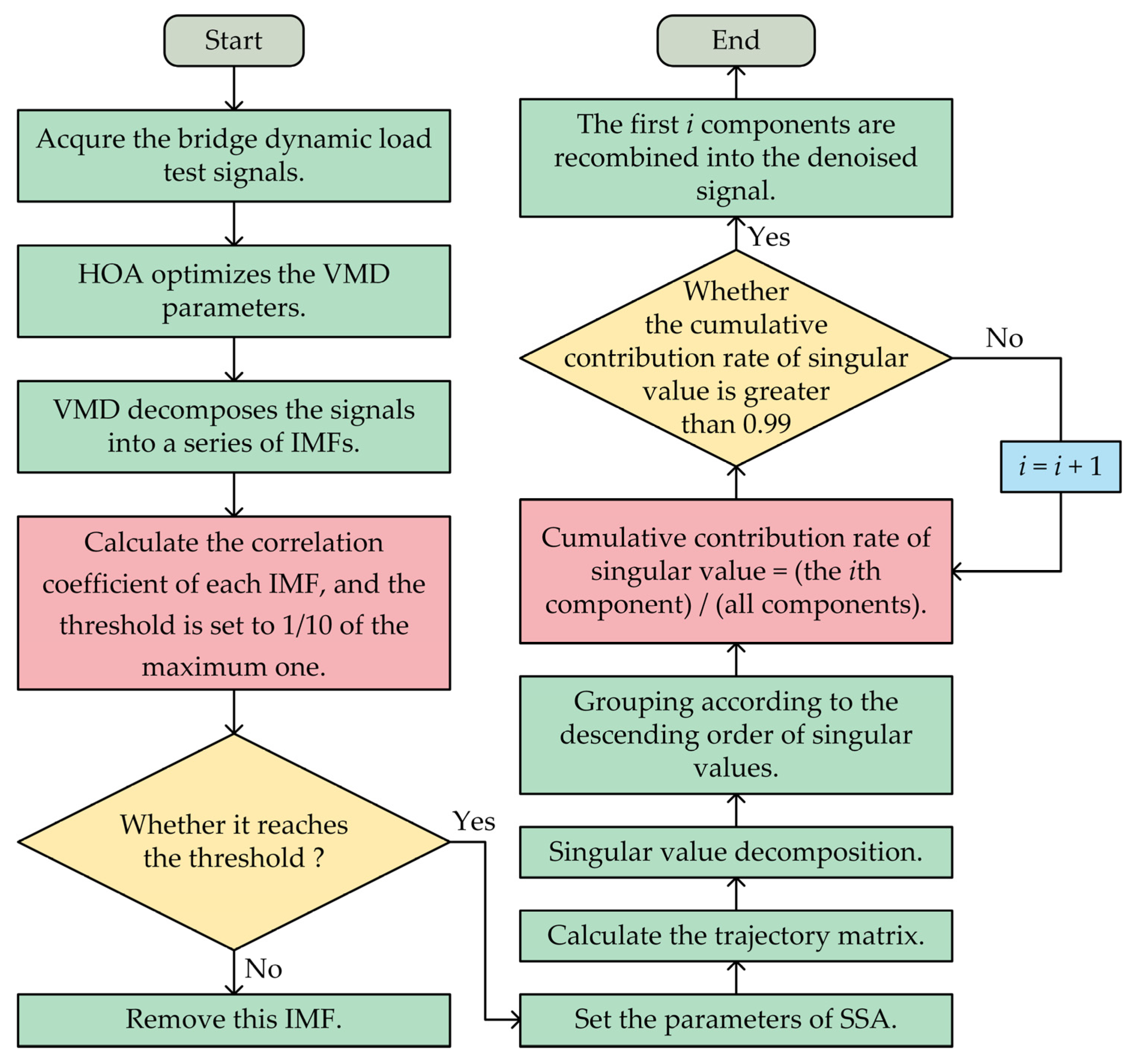
3.3. Singular Spectrum Analysis

While VMD effectively processes the noise in the bridge dynamic load test signal, residual local low-frequency oscillations often persist in the denoised output, which affects the accuracy and reliability of the test results. To overcome this phenomenon, SSA is introduced. The implementation of SSA is mainly divided into two complementary stages.

• Stage 1: Decomposition

The window length is set according to the number of sampling points $N$. Let $K=N-L+1$; the effective IMFs after VMD denoising are composed of one-dimensional time series $u_1,u_2,\dots ,u_N$ and reconstructed into Hankel matrix $U$:

$$U=\left[u_1,u_2,\dots ,u_N\right]={\left(u_{ij}\right)}_{i,j=1}^{L,K}=\left[\begin{array}{cccc}{u}_1& u_2& \cdots & u_K\\ u_2& u_3& \cdots & u_{K+1}\\ ⋮& ⋮& \ddots & ⋮\\ u_L& u_{L+1}& \cdots & u_N\end{array}\right]$$

(16)

The larger singular value of the singular value decomposition of matrix $U$ represents the larger energy contribution rate of the corresponding component. Let $Z=U{U}^T$; $U^T$ is the transpose of trajectory matrix $U$. The eigenvalues of the $Z$, which are also singular values, are ${\lambda }_1,{\lambda }_2,\dots ,{\lambda }_L$ in descending order. The rank of the trajectory matrix $U$ is $d=\max \left(i,{\lambda }_i>0\right)$, the left eigenvectors are $R_1,R_2,\dots ,R_L$, and the corresponding right eigenvectors are $M_i=U^T{R}_i/\sqrt{{\lambda }_i}\left(i=1,2,\dots ,d\right)$. The trajectory matrix $U$ is transformed into

$$U={\displaystyle \sum _{i=1}^d{U}_i}={\displaystyle \sum _{i=1}^d\sqrt{{\lambda }_i}{R}_i{M}_i^T}$$

(17)

• Stage 2: Recombination

$p_{ij}\left(1\le i\le L,1\le j\le K\right)$ are the elements in the matrix after sorting the $U_i$ in descending order according to the size of the singular value. The matrix $P_{L\times K}$ composed of these elements is diagonally averaged, and matrix $P$ is transformed into a time series with a length of $N$:

$$p_i=\left\{\begin{array}{l}{\displaystyle \frac{1}{i}}{\displaystyle \sum _{j=1}^k{p}_{j,i-j+1}^{*}}\\ {\displaystyle \frac{1}{L^{*}}}{\displaystyle \sum _{j=1}^{L^{*}}{p}_{j,i-j+1}^{*}}\\ {\displaystyle \frac{1}{N-i+1}}{\displaystyle \sum _{j=i-K^{*}+1}^{N-K^{*}+1}{p}_{j,i-j+1}^{*}}\end{array}\right.\begin{array}{l}1\le i\le L^{*}\\ \\ L^{*}\le I\le K^{*}\\ \\ K<i\le N\end{array}$$

(18)

where $L^{*}=\min \left(L,K\right)$ and $K^{*}=\max \left(L,K\right)$; if $L<K$, then $p_{ij}^{*}=p_{ij}$, else $p_{ij}^{*}=p_{ji}$.

Similar to VMD, the SSA contains two vital parameters as well: window length $L$ and reconstruction order $R$. These parameters govern the compromise between signal fidelity and noise suppression in bridge dynamic load test signals characterized by non-stationary vibration components and ambient noise interference. An oversized $L$ leads to the aliasing of singular value decomposition results, whereas an undersized $L$ will result in the loss of some effective signals. Empirical studies by Mahmoudvand et al. [29] discovered that when nearly half of the time series length $N$ is selected as the window length $L$, the maximum singular value is usually obtained. Therefore, this research sets the window length $L$ to $N/2$. The reconstruction order $R$, as the second important parameter, governing component retention during signal synthesis. Overestimation of $R$ will cause excessive noise retention, while underestimation discards effective signals. To resolve this trade-off, $R$ is determined according to the number of singular values with a cumulative contribution rate of more than 99%. The corresponding first $r$ feature vectors are selected for reconstruction to form $\overline{U}$. The calculation formula of the $i$th component contribution rate ${\eta }^i$ is as follows:

$${\eta }^i={\displaystyle \frac{{\lambda }_i}{{\displaystyle \sum _{i=1}^L{\lambda }_i}}}$$

(19)

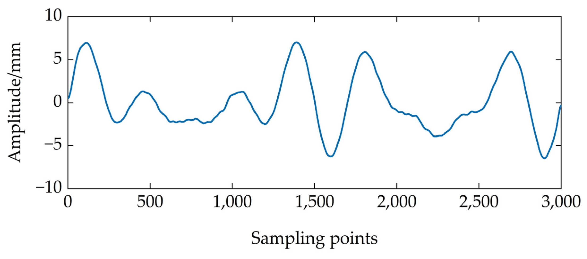
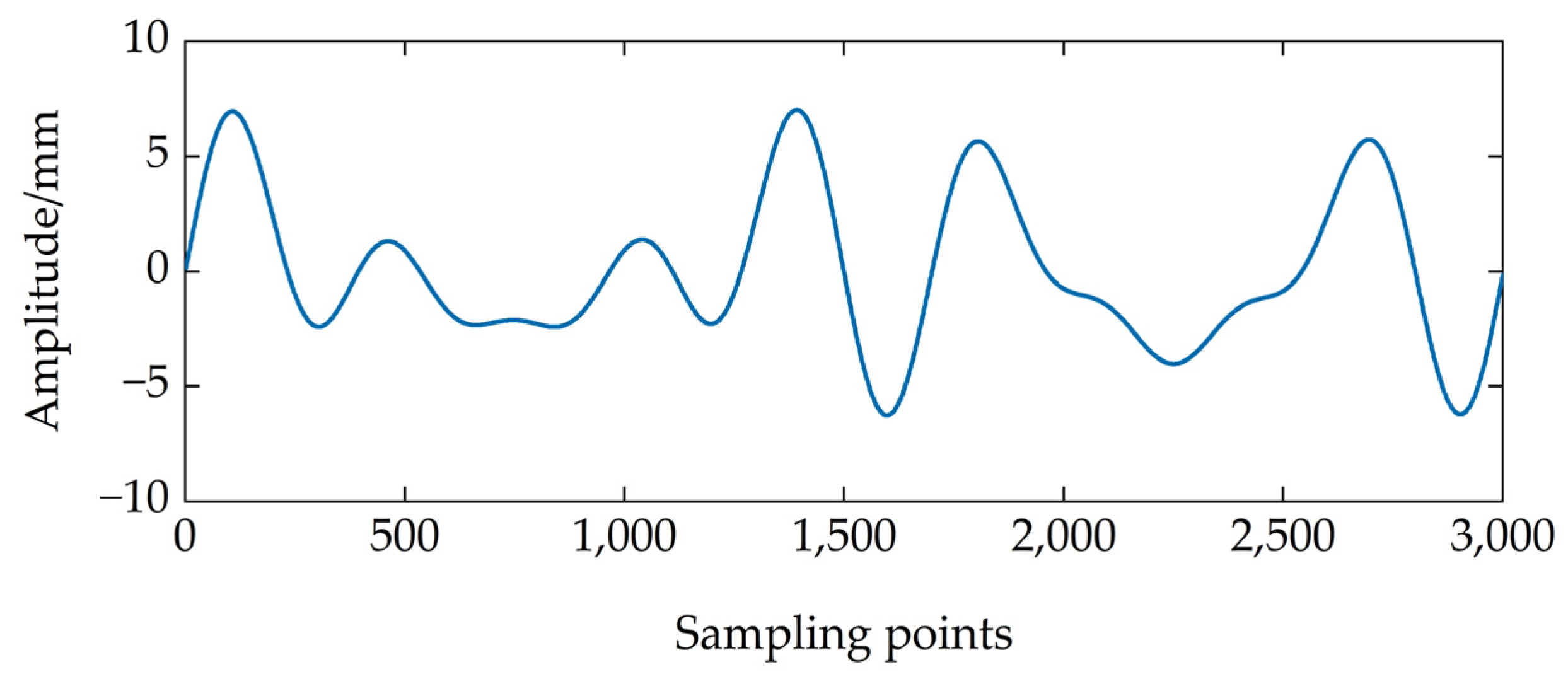
4. Simulation

To validate the denoising efficacy of the proposed HOA-optimized VMD-SSA framework, a systematic numerical investigation was conducted using MATLAB R2022a. Considering the typical frequency range of bridge signals is usually between 0.3 and 10 Hz, a random signal containing 1 Hz, 3 Hz, 5 Hz, 7 Hz, and 9 Hz frequency components were generated and superimposed according to specific formulas. To emulate realistic measurement conditions, we added Gaussian white noise $n$ with signal-to-noise ratio (SNR) of 5 dB, 10 dB, 15 dB, and 20 dB, respectively. The simulation signal $y$ is defined as follows, and the simulation of the signal is shown in Figure 4:

$$\left\{\begin{array}{l}{y}_1=3\sin \left(2\pi f_{1}t\right)·\sin \left(2\pi f_{2}t\right)\\ y_2=2\sin \left(2\pi f_{3}t\right)+3\sin \left(2\pi f_{4}t\right)+2\sin \left(2\pi f_{5}t\right)\\ y=y_1+y_2+n\end{array}\right.$$

(20)

where $t$ is the time vector; $f_1$, $f_2$, $f_3$, $f_4$, and $f_5$ are signal frequencies, which are 1, 3, 5, 7, and 9, respectively.

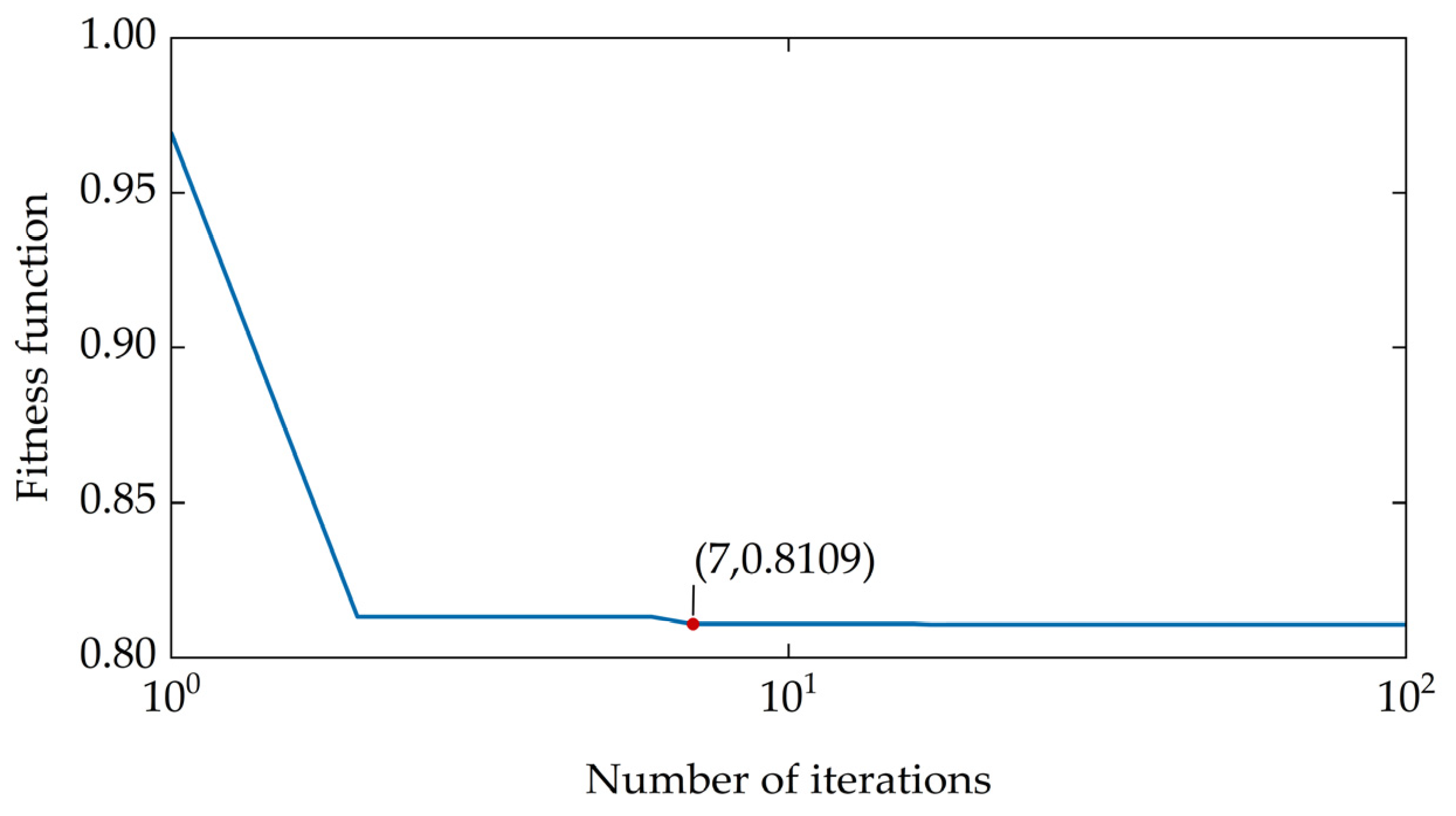
4.1. Process Analysis

Based on a comprehensive evaluation of the denoising performance at different noise levels, we selected the situation with an SNR of 15 dB as a demonstration case. The random noise-corrupted signal under this condition is processed through the HOA-VMD. The optimization results are illustrated in Figure 5. When the number of iterations reaches the seventh time, the fitness value is 0.8109, and the optimal parameter combination $\left[K,\alpha \right]$ = [20,1553] of VMD is output, which indicates the successful global optimum attainment. Then, the VMD decomposes the signal into 20 IMFs, as shown in Figure 6.

To systematically validate the unique advantages of HOA in optimizing VMD parameters, a comparative algorithmic framework was developed, including HOA, particle swarm optimization (PSO) [30], and gray wolf optimization (GWO) [31]. Experimental controls were implemented with identical computational constraints—population size ($N=30$), iteration limits ($T_{\max }=25$), and parametric search boundaries ($K\in$ [5,20], $\alpha \in$ [100,2500])—to ensure unbiased performance benchmarking.

The Pearson correlation coefficient index was used to compare the linear correlation between the two variables. Hence, the correlation coefficients between each IMF component and the original signal can be calculated to measure the similarity between each IMF and the original signal [32]. A higher correlation coefficient indicates stronger morphological consistency. The correlation coefficient of the $i$ th IMF is defined as

$$C{C}_i={\displaystyle \frac{E[u_i\left(t\right)·X\left(t\right)]-E[u_i\left(t\right)]·E[X\left(t\right)]}{\sqrt{D[u_i\left(t\right)]}·\sqrt{D[X\left(t\right)]}}}$$

(21)

where $u_i\left(t\right)$ is the $i$ th IMF component after VMD decomposition, $X\left(t\right)$ is the original signal, $E\left(·\right)$ is mathematical expectation, $D\left(·\right)$ is the mathematical variance, and the threshold of the correlation coefficient is set to 1/10 of the maximum correlation coefficient in the component.

The correlation coefficient of IMFs is calculated as shown in

Table 1. The correlation coefficient calculation of IMF1 to IMF20.

IMF	Correlation Coefficient	IMF	Correlation Coefficient
1	0.9833	11	0.0469
2	0.3481	12	0.0452
3	0.0623	13	0.0454
4	0.0530	14	0.0446
5	0.0528	15	0.0457
6	0.0523	16	0.0468
7	0.0527	17	0.0465
8	0.0501	18	0.0460
9	0.0475	19	0.0436
10	0.0459	20	0.0420

. The maximum correlation coefficient is 0.9833. Therefore, the threshold is set to 0.0983. We discarded IMF3 to IMF20 and superimposed the remaining IMF1 and IMF2 as the denoised signal, which is shown in Figure 7. The comparative denoising performance of HOA-VMD, PSO-VMD, and GWO-VMD, averaging over 10 Monte Carlo trial repetitions, is systematically demonstrated in

Table 2. Performance evaluation of HOA-VMD, PSO-VMD, and GWO-VMD.

Method	Best Parameter [$\mathit{K}$,$\mathit{\alpha }$]	Correlation Coefficient	Time/min
HOA-VMD	[20,1544]	0.9924	64.64
PSO-VMD	[20,1237]	0.9683	59.11
GWO-VMD	[20,1551]	0.9733	63.98

. The denoising results of PSO-VMD and GWO-VMD are depicted in Figure 8 and Figure 9, respectively. Notably, although the VMD-denoised signal approximates the original waveform in global morphological features, local oscillations still exist. This is because there are low-frequency noises in the denoised signal. To address this limitation, the second denoising is performed by SSA. Specifically, we input IMF1 and IMF2 into SSA for decomposition and reconstruction, and the refined signal is shown in Figure 10.

Table 2 presents a comparative analysis of denoising performance among HOA, PSO, and GWO, focusing on two critical metrics: Pearson correlation coefficients between denoised and pure reference signal, and computational optimization duration. The results reveal that the PSO and GWO demonstrate 8.56% and 1.02% reductions in optimization time, respectively, compared to HOA. However, the HOA-processed signal exhibits superior signal fidelity with 2.49% and 1.96% enhancements in correlation coefficients relative to PSO and GWO counterparts. This performance dichotomy indicates a fundamental trade-off between computational efficiency and signal preservation accuracy. While PSO and GWO achieve marginally faster convergence, parametric optimization prioritizes spectral fidelity over computational speed in bridge structural health monitoring. This prioritization is essential because minor modal parameter deviations may indicate early-stage bridge structural degradation [33]. Consequently, HOA is selected to optimize the VMD parameters, as this approach provides the necessary balance between computational feasibility and precision required for infrastructure monitoring applications.

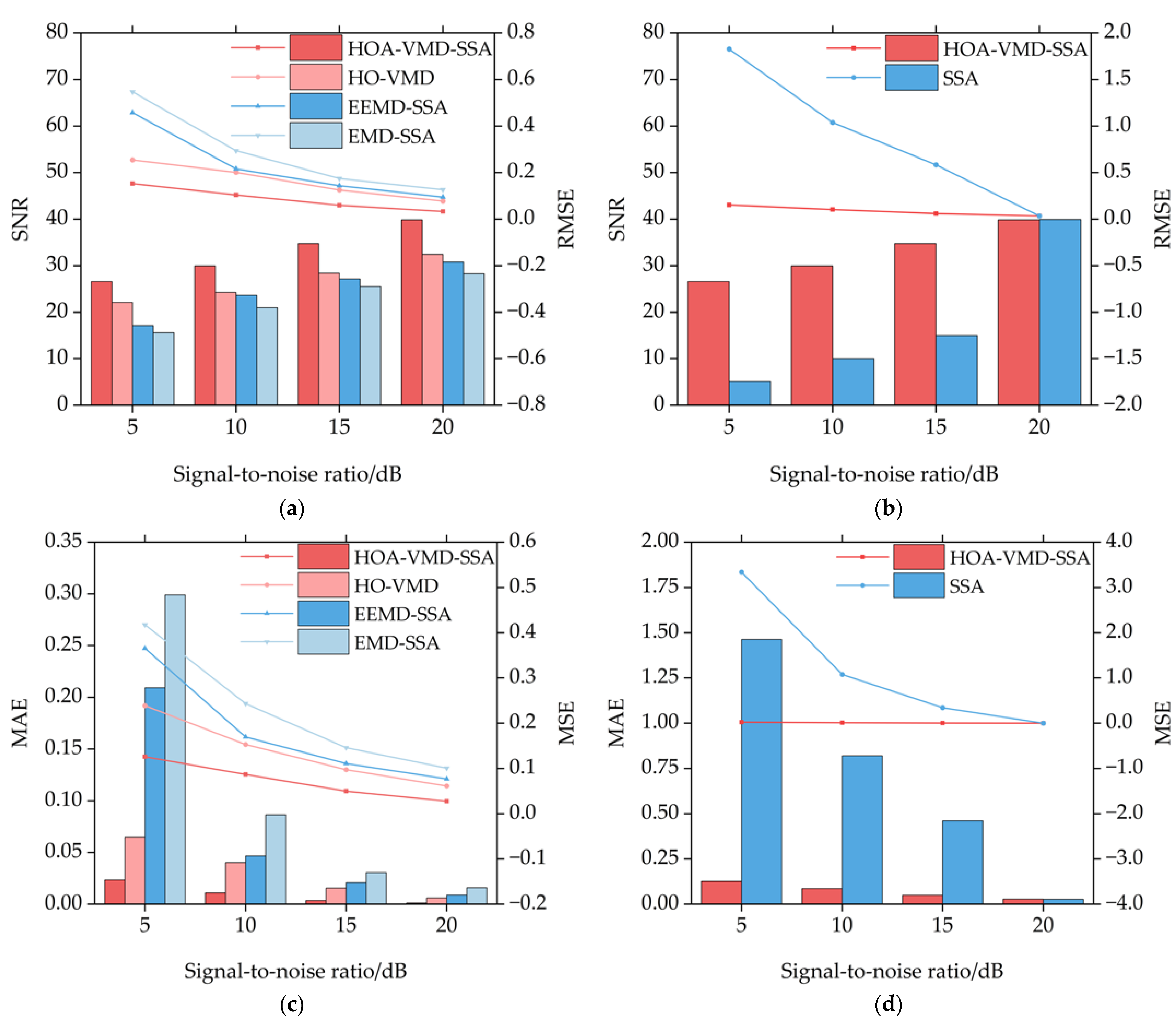
4.2. Results Analysis

In Figure 11, these two signals have a high degree of curve fitting, only slight deviation exists locally, and the signal oscillation phenomenon is significantly reduced.

This research develops a quadruple-metric framework incorporating root mean square error, signal-to-noise ratio, mean square error, and mean absolute error to evaluate the comparative performance of different denoising methods:

• Index 1: Root Mean Square Error (RMSE)

The RMSE is an indicator to measure the accuracy of the prediction. It emphasizes the large error and intuitively reflects the accuracy of the model prediction. Lower RMSE values correspond to more reliable model prediction [34,35]. Defined as follows:

$$RMSE=\sqrt{{\displaystyle \frac{1}{n}}{{\displaystyle \sum _{i=1}^n\left(u\left(i\right)-u\left(\widehat{i}\right)\right)}}^2}$$

(22)

• Index 2: Signal-to-Noise Ratio (SNR)

The SNR is an indicator of signal clarity. It emphasizes the contrast between the intensity of useful information in the signal and the intensity of interference noise. Higher SNR values correspond to purer signal [36]. Defined as follows:

$$SNR=10\times \lg \left({\displaystyle \frac{{\displaystyle \sum _{i=1}^n{u}^2\left(i\right)}}{{\displaystyle \sum _{i=1}^n{\left(u\left(i\right)-u\left(\widehat{i}\right)\right)}^2}}}\right)$$

(23)

• Index 3: Mean Square Error (MSE)

The MSE is a widely used metric to quantify the accuracy of prediction models. It calculates the average squared difference between predicted and true values, thereby assigning higher weight to larger errors. Lower MSE values indicate better model performance in minimizing prediction deviations [37]. Defined as follows:

$$MSE={\displaystyle \frac{1}{n}}{{\displaystyle \sum _{i=1}^n\left(u\left(i\right)-u\left(\widehat{i}\right)\right)}}^2$$

(24)

• Index 4: Mean Absolute Error (MAE)

The MAE quantifies the average magnitude of prediction errors by computing the absolute differences between predicted and true values. Unlike RMSE and MSE, it treats all errors uniformly without amplifying larger deviations. Lower MAE values indicate higher consistency between model predictions and ground truth, reflecting the model’s stability in practical applications [38]. Defined as follows:

$$MAE={\displaystyle \frac{1}{n}}{\displaystyle \sum _{i=1}^n\left|u\left(i\right)-u\left(\widehat{i}\right)\right|}$$

(25)

where $u\left(i\right)$ is the original signal, $u\left(\widehat{i}\right)$ is the signal after denoising, and $n$ is the number of sampling points.

After applying five distinct denoising methods to the simulation signals with different levels of noise, this research quantitatively evaluates the denoising effect and obtains the RMSE and SNR corresponding to each method, as summarized in

Table 3. Comparison of RMSE and SNR of five denoising methods at different noise levels.

Denoising Method	5 dB		10 dB		15 dB		20 dB
	RMSE	SNR	RMSE	SNR	RMSE	SNR	RMSE	SNR
HOA-VMD-SSA	0.1530	26.62	0.1042	29.95	0.0598	34.78	0.0333	39.85
HOA-VMD	0.2545	22.13	0.2008	24.27	0.1250	28.38	0.0778	32.45
EEMD-SSA	0.4575	17.11	0.2159	23.63	0.1437	27.16	0.0946	30.79
EMD-SSA	0.5468	15.56	0.2939	20.95	0.1749	25.46	0.1266	28.27
SSA	1.8271	5.08	1.0379	9.99	0.5836	14.99	0.0330	39.93

and

Table 4. Comparison of MSE and MAE of five denoising methods at different noise levels.

Denoising Method	5 dB		10 dB		15 dB		20 dB
	MSE	MAE	MSE	MAE	MSE	MAE	MSE	MAE
HOA-VMD-SSA	0.0234	0.1257	0.0109	0.0867	0.0036	0.0498	0.0011	0.0278
HOA-VMD	0.0648	0.2388	0.0403	0.1530	0.0156	0.0971	0.0061	0.0611
EEMD-SSA	0.2093	0.3654	0.0466	0.1695	0.0207	0.1107	0.0089	0.0770
EMD-SSA	0.2990	0.4174	0.0864	0.2434	0.0306	0.1458	0.0160	0.1007
SSA	3.3383	1.4630	1.0772	0.8205	0.3406	0.4614	0.0011	0.0274

.

According to the data from Table 3 and Table 4, dual comparative analyses were performed to validate methodological superiority:

• Algorithmic Hybridization Contrast: The proposed HOA-VMD-SSA, HOA-VMD, EEMD-SSA, and EMD-SSA;
• Component Efficacy Verification: The proposed HOA-VMD-SSA and SSA.

Dual-axis visualization was employed to enhance interpretative clarity: RMSE and MSE are represented by a line chart to track the dynamic change of noise reduction level, while SNR and MAE are represented by a histogram to quantify residual distortion. A biaxial columnar line chart was drawn, as shown in Figure 12.

In the comparison experiment for the denoising effect at different noise levels, the denoising method proposed in this research achieves the lowest RMSE, MSE, and MAE, as well as the highest SNR. Notably, in a high-level noise environment, the conventional SSA method exhibits significant performance degradation. While SSA slightly outperforms the proposed method at the 20 dB noise level, this advantage diminishes as the noise level increases. The quantitative evaluations confirm the superiority of the proposed method in this research, achieving an average 16.22% reduction in RMSE, an average 62.02% diminution in MSE, an average 43.74% decrease in MAE, and an average 2.51% improvement in SNR compared to other algorithmic hybridization approaches.

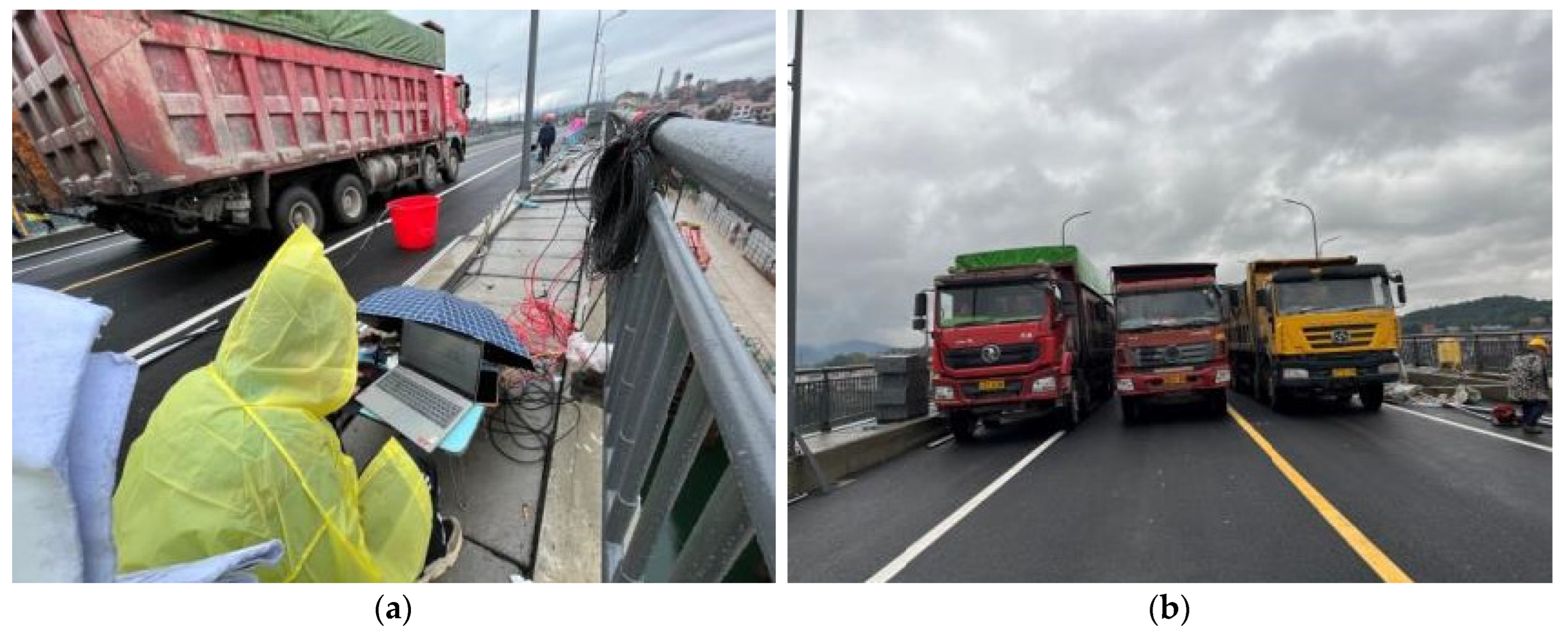
5. Experiment

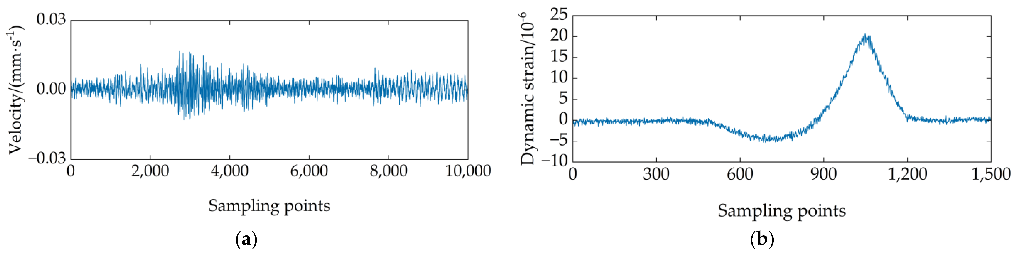
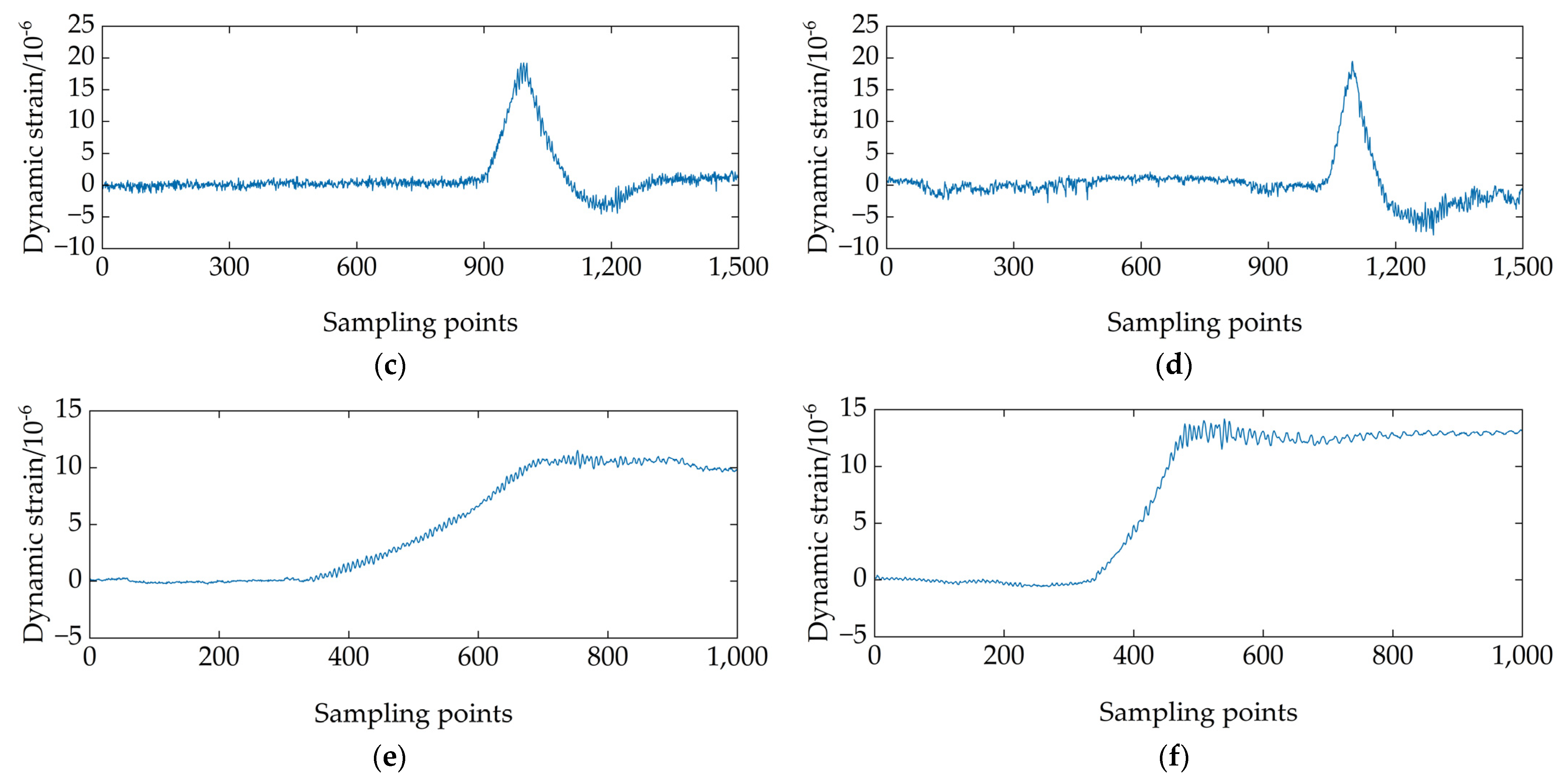
5.1. Signal Acquisition

A prestressed variable cross-section continuous beam bridge located in Hunan Province, China was selected as the research subject to validate the proposed denoising method. The bridge had to be dismantled and rebuilt due to the cracking of the bridge body. After completion in 2024, it once again became an important transportation hub connecting the two sides of the river. To prevent the bridge having serious degradation again and ensure its long-term stable operation, the overall performance and operational state were evaluated. This was achieved by measuring the natural and forced vibration signals at the maximum bending moment section under dynamic loads. The data acquisition was completed by the DH5922N dynamic resistance strain acquisition system.

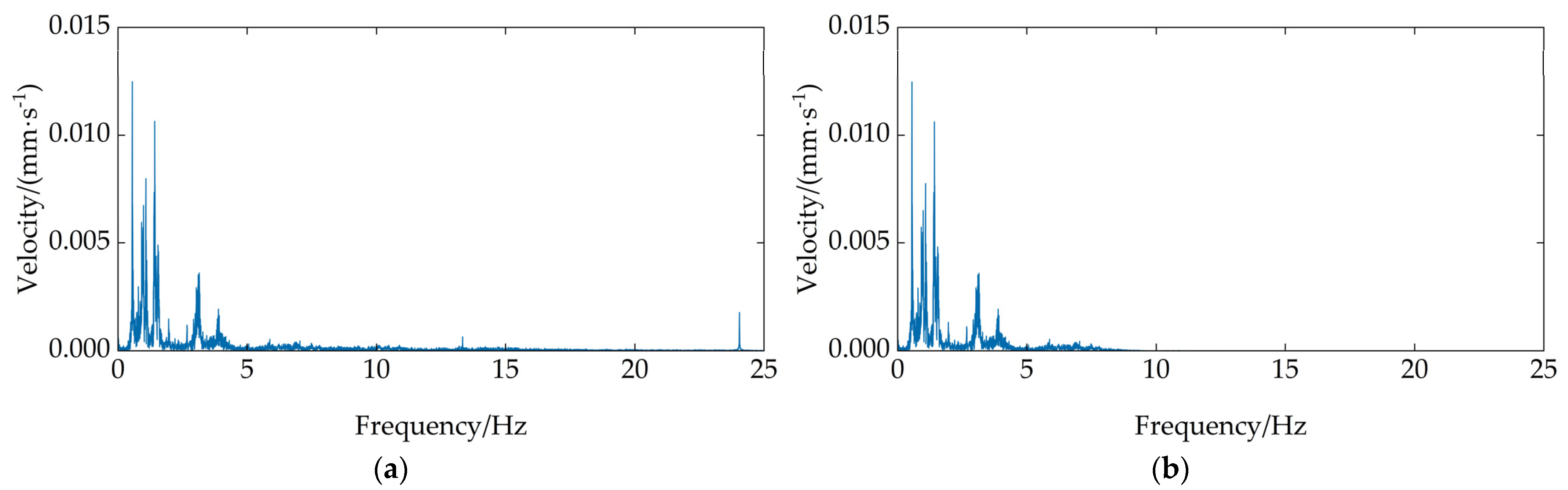
5.2. Signal Processing

As shown in Figure 13, a series of dynamic load tests were conducted on the target bridge. The goal was to comprehensively evaluate the structure’s dynamic response characteristics under operational loading conditions. The test protocol is detailed in

Table 5. The protocol of dynamic load test of bridge.

Test Project	Details	Sampling Frequency
Fundamental frequency detection	Measure the natural vibration frequency of the bridge structure that is applied by the natural environment. Provide a basis for evaluating the dynamic characteristics of the bridge.	100 Hz
Driving vibration excitation	Simulate the bridge response under normal driving conditions. The test speeds are set to 10 km/h, 20 km/h, and 30 km/h, respectively, to cover the influence of different driving speeds on the bridge structure.	20 Hz
Braking vibration excitation	Simulate the bridge response under emergency braking. The test speeds are 10 km/h and 20 km/h, respectively, to evaluate the structural stability of the bridge in emergency situations.	20 Hz

. To validate the engineering efficacy of the denoising method presented in this research, the fifth span of the main bridge, which exhibits a heightened sensitivity to traffic-induced vibrations, was subjected for comparative analysis. This selection aims to evaluate the denoising effect of the proposed method in practical applications.

The main primary dynamic characteristics of bridge structures, including natural frequency and damping ratio, can be extracted through operational modal analysis using environmental vibration signals. However, the fundamental frequency signal in Figure 14 has noise interference and poor readability, which may affect the accuracy of analysis results. To further evaluate the structural performance of the bridge, the impact coefficient of the bridge is calculated by using the signals collected by the driving and braking tests. The impact coefficient is defined as follows [39]:

$$\mu ={\displaystyle \frac{f_{d\max }}{f_{j\max }}}-1$$

(26)

where $f_{d\max }$ is the maximum dynamic strain amplitude and $f_{j\max }$ is the vertex value of the waveform amplitude center trajectory.

In Figure 14, according to the calculation formula of the impact coefficient, amplitude determination becomes challenging due to the sudden change of the signal at the peak value. In addition, given the lack of original noiseless signal, to improve the reliability of the analysis, the variance contribution rate (VCR) is selected instead of the correlation coefficient to screen the IMFs [40]. The smaller VCR indicates that the IMF contains less effective signal components. The VCR of the $i$th IMF is defined as

$$VC{R}_i={\displaystyle \frac{\left[\frac{1}{N}{\displaystyle \sum _{t=1}^n{u}_i{\left(t\right)}^2}-{\left(\frac{1}{N}{\displaystyle \sum _{t=1}^N{u}_i\left(t\right)}\right)}^2\right]}{{\displaystyle \sum _{t=1}^N\left[\frac{1}{N}{\displaystyle \sum _{t=1}^n{u}_i{\left(t\right)}^2}-{\left(\frac{1}{N}{\displaystyle \sum _{t=1}^N{u}_i\left(t\right)}\right)}^2\right]}}}$$

(27)

where $N$ is the number of sampling points and $n$ is the number of IMFs. Remove the IMF that does not meet VCR $\le$ 0.01, complete the initial denoising, and input the remaining IMF to SSA for secondary denoising.

5.3. Results Analysis

The collected signals are processed separately by the method. As the fundamental frequency signal demonstrated in Figure 15, a comparative time-domain analysis reveals that there is little difference in amplitude between raw and denoised signal. This phenomenon indicates that the denoising process selectively targets high-amplitude noise components while preserving structural vibration characteristics. This selective mechanism confirms the algorithm’s capability to maintain critical signal integrity during noise suppression.

Frequency-domain analysis is an effective signal processing analysis tool that can reveal the energy distribution of signal at different frequencies. Thus, to highlight the denoising effect of this method from another perspective, select the frequency domain diagram of the fundamental frequency signal before and after denoising for further validation. As shown in Figure 16, the proposed denoising method selectively preserves the 0–10 Hz spectral components while achieving effective suppression of high-frequency noise above 10 Hz. These quantitative metrics demonstrate the proposed method’s precision in discriminating structural response signatures from environmental noise.

Due to the inability to obtain the pure signals without noise, RMSE and SNR indicators are no longer applicable. Therefore, two new indices are introduced to comprehensively evaluate the denoising effect.

• Index 1: Normalization Shannon Entropy Ratio (NSER)

Shannon entropy can be used to measure the uncertainty of information combined with signal normalization [41]. The smaller NSER represents the better denoising effect, which is defined as

$$NSER={\displaystyle \frac{S\left(\left|N\left(x\left(\widehat{i}\right)\right)\right|\right)}{S\left(\left|N\left(x\left(i\right)\right)\right|\right)}}$$

(28)

where $S\left(·\right)$ is Shannon entropy function, $N\left(·\right)$ is the most value normalization function, $x\left(i\right)$ is a noisy signal, and $x\left(\widehat{i}\right)$ is the denoised signal.

• Index 2: Noise Suppression Ratio (NSR)

NSR is an index to measure the effect of noise suppression that is used to quantify and evaluate the effectiveness of noise suppression technology [42]. A smaller NSER indicates the higher noise suppression rate, which is defined as

$$NSR=10\left(\lg {\sigma }_1^2-\lg {\sigma }_2^2\right)$$

(29)

where ${\sigma }_1$ and ${\sigma }_2$ are the standard deviations of the signal before and after denoising, respectively.

Three distinct signal types were selected for systematic evaluation:

• The bridge fundamental frequency signal;
• The 30 km/h barrier-free traffic signal;
• The 10 km/h braking signal.

These datasets were subjected to denoising procedures using the conventional EMD-SSA and EEMD-SSA methodologies. Whereas the HOA-VMD denoising outputs are derived from HOA-VMD-SSA. The NSER and NSR indices of each method were calculated to objectively assess denoising performance. Notably, the SSA is excluded from consideration due to its great sensitivity to noise level, as demonstrated in the simulation. As tabulated in

Table 6. Index calculation of denoising methods.

Denoising Method	Fundamental Frequency Signal		30 km/h Barrier-Free Traffic Signal		10 km/h Braking Signal
	NSER	NSR	NSER	NSR	NSER	NSR
HOA-VMD-SSA	0.8840	0.1592	0.7202	0.1965	0.7797	0.1565
HOA-VMD	0.9432	0.1580	0.7693	0.1823	0.8021	0.1495
EEMD-SSA	0.9601	0.1537	0.8866	0.1751	0.8759	0.1452
EMD-SSA	0.9845	0.1486	0.9202	0.1655	0.9013	0.1336

, the proposed method demonstrated superior performance across both indices, achieving NSER reductions of 12.81% and NSR improvements of 8.44% compared to traditional methods. These enhancements confirm the enhanced signal fidelity and operational efficiency of the proposed method in this research.

6. Discussion

While the proposed HOA-VMD-SSA framework demonstrates effective noise suppression in bridge dynamic load test signals, three methodological limitations warrant refinement for enhanced robustness:

• Although the current framework utilizes HOA for VMD parameter optimization, its failure to conduct comparative analyses with canonical metaheuristic optimizers (e.g., whale optimization algorithm, genetic algorithms) undermines methodological validation rigor. Furthermore, HOA’s triple-phase optimization mechanism raises unresolved questions regarding computational efficiency trade-offs in large-scale engineering applications.
• SSA denoising performance exhibits great dependence on the window length and reconstruction order. Despite the parameters being selected based on existing research, it does not consider whether the requirements of signal characteristics and algorithm combination on parameters will change, which raises questions about whether the chosen parameters are applicable to bridge signals. Therefore, it is necessary to pay continuous attention to the parameter selection of SSA.
• In the simulation experiment of this research, SSA shows characteristics of poor adaptability to noisy environments. This may result from the complex high-level white noise environment; some white noise is superimposed into impulse noise. As SSA has limited denoising ability for impulse noise, this leads to the distortion of denoising signals.
• In the present study, while the selection of VMD parameters was adaptively selected by the HOA, the parameter configuration for the SSA remained empirically determined through manual intervention. Therefore, it is paramount to validate the possibility of SSA parameters being optimized by meta-heuristic algorithms, which in turn allows for us to verify the adaptability of SSA for denoising bridge dynamic load test signals.

Regarding applicability, the proposed method was validated solely on prestressed continuous beam bridge load tests. Future research should prioritize other bridge types with distinct vibration signatures, such as cable-stayed, suspension, arch bridges, etc. Meanwhile, the denoising potential of the proposed method in other fields such as seismic and electromagnetic signals needs to be further developed and verified.

7. Conclusions

To address noise interference in bridge dynamic load testing, this research develops a hybrid signal processing method combining the HOA, VMD, and SSA. The proposed method effectively removes the noise in the bridge dynamic load test signal while suppressing local low-frequency oscillations that persist in conventional VMD outputs. Numerical simulations and engineering applications demonstrate three key advancements:

• SSA resolves persistent low-frequency oscillations in primary VMD outputs through an internal decomposition and reconstruction mechanism. It can effectively identify and separate the periodic and trending components in the signal, thereby eliminating oscillations and improving signal readability.
• Compared to other denoising methods, the proposed HOA-VMD-SSA achieves 16.2% RMSE reduction, 2.51% SNR enhancement, 62.02% MSE slump, and 43.74% MAE decline in numerical simulation. These results indicate that the proposed method in this research shows outstanding denoising stability under different noise level environments.
• Engineering validation shows that compared with other denoising methods, the proposed method in this research achieves a 12.8% NSER decrease and 8.44% NSR improvement, which shows that the proposed HOA-VMD-SSA is suitable for bridge dynamic load test signal denoising.

References

- Hu, C.W.; Luo, W.B.; Chen, S.C. Evaluation of bearing capacity of reinforced stone arch bridge based on dynamic load test. IOP Conf. Ser. Earth Environ. Sci. 2020, 546, 042069. [Google Scholar] [CrossRef]
- Gatti, M. Structural health monitoring of an operational bridge: A case study. Eng. Struct. 2019, 195, 200–209. [Google Scholar] [CrossRef]
- Sun, Z.L.; Lu, J.G. An ultrasonic signal denoising method for EMU wheel trackside fault diagnosis system based on improved threshold function. IEEE Access 2021, 9, 96244–96256. [Google Scholar] [CrossRef]
- Kordestani, H.; Zhang, C.W.; Masri, S.F.; Shadabfar, M. An empirical time-domain trend line-based bridge signal decomposing algorithm using Savitzky-Golay filter. Struct. Control Health Monit. 2021, 28, e2750. [Google Scholar] [CrossRef]
- Liu, X.L.; Wang, H.; Huang, M.; Yang, W.X. An improved second-order blind identification (SOBI) signal de-noising method for dynamic deflection measurements of bridges using ground-based synthetic aperture radar (GBSAR). Appl. Sci. 2019, 9, 3561. [Google Scholar] [CrossRef]
- Fang, Z.; Yu, J.Y.; Meng, X.L. Modal parameters identification of bridge structures from GNSS data using the improved empirical wavelet transform. Remote Sens. 2021, 13, 3375. [Google Scholar] [CrossRef]
- Huang, N.E.; Shen, Z.; Long, S.R.; Wu, M.C.; Shih, H.H.; Zheng, Q.A.; Yen, N.C.; Tung, C.; Liu, H.H. The empirical mode decomposition and the Hilbert spectrum for nonlinear and non-stationary time series analysis. Proc. R. Soc. Lond. A 1998, 454, 903–995. [Google Scholar] [CrossRef]
- Ge, H.Q.; Chen, G.B.; Yu, H.C.; Chen, H.B.; An, F.P. Theoretical analysis of empirical mode decomposition. Symmetry 2018, 10, 623. [Google Scholar] [CrossRef]
- Wu, Z.; Huang, N.E. Ensemble empirical mode decomposition: A noise-assisted data analysis method. Adv. Adapt. Data Anal. 2009, 1, 1–41. [Google Scholar] [CrossRef]
- Dragomiretskiy, K.; Zosso, D. Variational mode decomposition. IEEE Trans. Signal Process. 2014, 62, 531–544. [Google Scholar] [CrossRef]
- Zhou, J.; Guo, X.M.; Wang, Z.J.; Du, W.H.; Wang, J.Y.; Han, X.F.; Wang, J.T.; He, G.F.; He, H.H.; Xue, H.L.; et al. Research on fault extraction method of variational mode decomposition based on immunized fruit fly optimization algorithm. Entropy 2019, 21, 400. [Google Scholar] [CrossRef] [PubMed]
- Ji, H.X.; Huang, K.; Mo, C.Q. Research on the application of variational mode decomposition optimized by snake optimization algorithm in rolling bearing fault diagnosis. Shock Vib. 2024, 2024, 5549976. [Google Scholar] [CrossRef]
- Fang, T.; Ma, L.; Zhang, H.K. Research on fault diagnosis method with adaptive artificial gorilla troops optimization optimized variational mode decomposition and support vector machine parameters. Machines 2024, 12, 637. [Google Scholar] [CrossRef]
- Nassef, M.G.A.; Hussein, T.M.; Mokhiamar, O. An adaptive variational mode decomposition based on sailfish optimization algorithm and Gini index for fault identification in rolling bearings. Measurement 2021, 173, 108514. [Google Scholar] [CrossRef]
- Zhang, X.; Miao, Q.; Zhang, H.; Wang, L. A parameter-adaptive VMD method based on grasshopper optimization algorithm to analyze vibration signals from rotating machinery. Mech. Syst. Signal Process. 2018, 108, 58–72. [Google Scholar] [CrossRef]
- Amiri, M.H.; Hashjin, N.M.; Montazeri, M.; Mirjalili, S.; Khodadadi, N. Hippopotamus optimization algorithm: A novel nature-inspired optimization algorithm. Sci. Rep. 2024, 14, 5032. [Google Scholar] [CrossRef]
- Maurya, P.; Tiwari, P.; Pratap, A. Application of the hippopotamus optimization algorithm for distribution network reconfiguration with distributed generation considering different load models for enhancement of power system performance. Electr. Eng. 2024, 2024, 1–38. [Google Scholar] [CrossRef]
- Chen, Y.Z.; Wu, F.; Shi, L.J.; Li, Y.; Qi, P.; Guo, X. Identification of sub-synchronous oscillation mode based on HO-VMD and SVD-regularized TLS-prony methods. Energies 2024, 17, 5067. [Google Scholar] [CrossRef]
- Lei, W.; Wang, G.; Wan, B.Q.; Min, Y.Z.; Wu, J.M.; Li, B.P. High voltage shunt reactor acoustic signal denoising based on the combination of VMD parameters optimized by coati optimization algorithm and wavelet threshold. Measurement 2024, 224, 113854. [Google Scholar] [CrossRef]
- Li, H.; Li, S.S.; Sun, J.; Huang, B.C.; Zhang, J.Q.; Gao, M.Y. Ultrasound signal processing based on joint GWO-VMD wavelet threshold functions. Measurement 2024, 226, 114143. [Google Scholar] [CrossRef]
- Zhou, Y.T.; Zhu, Z.L. A hybrid method for noise suppression using variational mode decomposition and singular spectrum analysis. J. Appl. Geophys. 2019, 161, 105–115. [Google Scholar] [CrossRef]
- Li, H.; Liu, T.; Wu, X.; Chen, Q. An optimized VMD method and its applications in bearing fault diagnosis. Measurement 2020, 166, 108185. [Google Scholar] [CrossRef]
- Gan, M.; Pan, H.D.; Chen, Y.P.; Pan, S.Q. Application of the variational mode decomposition (VMD) method to river tides. Estuar. Coast. Shelf Sci. 2021, 261, 107570. [Google Scholar] [CrossRef]
- Jia, B.; Li, S.L.; Liu, D.S.; Wu, S.F. Application of low-frequency processing method based on VMD algorithm in blasting signal processing. Shock Vib. 2022, 2022, 5779714. [Google Scholar] [CrossRef]
- Gong, T.K.; Yuan, X.H.; Yuan, Y.B.; Lei, X.H.; Wang, X. Application of tentative variational mode decomposition in fault feature detection of rolling element bearing. Measurement 2019, 135, 481–492. [Google Scholar] [CrossRef]
- Li, Z.P.; Chen, J.L.; Zi, Y.Y.; Pan, J. Independence-oriented VMD to identify fault feature for wheel set bearing fault diagnosis of high speed locomotive. Mech. Syst. Signal Process. 2017, 85, 512–529. [Google Scholar] [CrossRef]
- Zhang, X.; Li, D.Q.; Li, J.; Li, Y. Grey wolf optimization-based variational mode decomposition for magnetotelluric data combined with detrended fluctuation analysis. Acta Geophys. 2022, 70, 111–120. [Google Scholar] [CrossRef]
- Chao, Z.X.; Yang, Y.; He, C.B.; Liu, Y.B.; Liu, X.Z.; Cao, Z. Feature extraction based on hierarchical improved envelope spectrum entropy for rolling bearing fault diagnosis. IEEE Trans. Instrum. Meas. 2023, 72, 1–12. [Google Scholar]
- Mahmoudvand, R.; Zokaei, M. On the singular values of the Hankel matrix with application in singular spectrum analysis. Chil. J. Stat. 2012, 3, 43–56. [Google Scholar]
- Wu, C.Y.; Duan, Y.Y.; Wang, H. Signal denoising of traffic speed deflectometer measurement based on partial swarm optimization-variational mode decomposition method. Sensors 2024, 24, 3708. [Google Scholar] [CrossRef]
- Cao, L.; Zhou, H.L.; Peng, W.B.; Liu, J.P.; Chen, Y.F. Analytical analysis on the static support reactions of single-column pier bridges using the grey wolf optimizer. Structures 2023, 55, 2003–2012. [Google Scholar] [CrossRef]
- Mao, M.H.; Chang, J.; Sun, J.C.; Lin, S.; Wang, Z.H. Research on VMD-based adaptive TDLAS signal denoising method. Photonics 2023, 10, 674. [Google Scholar] [CrossRef]
- Lin, F.Z.; Scherer, R.J. Concrete bridge damage detection using parallel simulation. Autom. Constr. 2020, 119, 103283. [Google Scholar] [CrossRef]
- Jiang, W.G.; You, W. A combined denoising method of empirical mode decomposition and singular spectrum analysis applied to Jason altimeter waveforms: A case of the Caspian Sea. Geod. Geodyn. 2022, 13, 327–342. [Google Scholar] [CrossRef]
- Wang, X.G.; Li, W.H.; Ma, M.; Yang, F.; Song, S. Bridge damage identification based on encoded images and convolutional neural network. Buildings 2024, 14, 3104. [Google Scholar] [CrossRef]
- Fu, J.J.; Cai, F.Y.; Guo, Y.H.; Liu, H.D.; Niu, W.T. An improved VMD-based denoising method for time domain load signal combining wavelet with singular spectrum analysis. Math. Probl. Eng. 2020, 2020, 1485937. [Google Scholar] [CrossRef]
- Asgarkhani, N.; Kazemi, F.; Jankowski, R. Machine learning-based prediction of residual drift and seismic risk assessment of steel moment-resisting frames considering soil-structure interaction. Comput. Struct. 2023, 289, 107181. [Google Scholar] [CrossRef]
- Wang, D.M.; Zhu, L.J.; Yue, J.K.; Lu, J.Y.; Li, D.W.; Li, G.F. Application of variational mode decomposition based on particle swarm optimization in pipeline leak detection. Eng. Res. Express 2020, 2, 045036. [Google Scholar] [CrossRef]
- Kim, C.; Kawatani, M.; Kwon, Y. Impact coefficient of reinforced concrete slab on a steel girder bridge. Eng. Struct. 2007, 29, 576–590. [Google Scholar] [CrossRef]
- Peng, K.; Guo, H.Y.; Shang, X.Y. EEMD and multiscale PCA-based signal denoising method and its application to seismic P-phase arrival picking. Sensors 2021, 21, 5271. [Google Scholar] [CrossRef]
- Zhang, J.; He, J.J.; Long, J.C.; Yao, M.; Zhou, W. A new denoising method for UHF PD signals using adaptive VMD and SSA-based shrinkage method. Sensors 2019, 19, 1594. [Google Scholar] [CrossRef] [PubMed]
- Li, L.A.; Wei, X.L. Suppression method of partial discharge interferences based on singular value decomposition and improved empirical mode decomposition. Energies 2021, 14, 8579. [Google Scholar] [CrossRef]