Abstract
Most of Italy’s residential building stock predates contemporary structural safety and energy efficiency regulatory frameworks. Today, policymakers face the challenge of choosing whether to prioritise renovation or opt for demolition and reconstruction; both options carry significant socio-economic and environmental consequences and require extensive knowledge of the built heritage. However, detailed architecture-specific data remain scarce, as existing databases lack granular information. Moreover, traditional urban-level knowledge mapping approaches may be resource-intensive. To address this data gap, this study proposes a semi-automated methodology for generating graph-based digital models representing residential building floor plans. Using graph theory, floor spatial layouts are mapped into connectivity graphs and transformed into topological models. These models are enriched with functional data about spaces by assigning conditional topological rules based on node centrality metrics. The method was tested on 98 buildings in Bologna, Italy, yielding an 89.8% success rate and demonstrating its effectiveness in data-limited contexts. The resulting dataset facilitates the analysis of floor spatial configurations and the extraction of geometric attributes, laying the foundation for future analyses that will integrate machine learning techniques for functional detection and typological clustering.
1. Introduction
Among Italy’s heterogeneous urban fabrics, the residential building stock is estimated at around 30 million units [1]. Approximately 70% of these structures were constructed before the 1970s, a period preceding the establishment of modern regulatory frameworks for seismic safety and energy performance. In contrast, only about 2 million houses were built after the introduction of the most recent building regulations in the early 2000s. Consequently, almost all existing residences fail to comply with current regulatory requirements.
In particular, the dwellings built between the 1940s and 1960s are characterised by intrinsic construction and architectural features—related to their structural systems, their low construction quality, the uncertainty in the definition of their structural safety and the urban and architectural conformation of the areas where they are located—that make them particularly inadequate for contemporary requirements. Only radical interventions, which are often complex to enforce, can restore these deficiencies completely and, above all, these interventions have high costs, complex execution, or in some cases are incompatible with the requirements needed to preserve listed buildings. Consequently, a key question confronting policymakers is whether to focus on the preservation/renovation of this heritage or opt instead for demolition/reconstruction strategies. Both approaches have socio-economic and environmental implications, necessitating a comprehensive knowledge of this heritage’s physical, typological, and construction characteristics for informed decision-making.
Acquiring detailed, building-specific knowledge using traditional mapping methods is complex and resource-intensive. Although existing digital databases—such as the ISTAT database and municipal Geographic Information Systems (GISs)—can facilitate data collection, they often provide only general information about buildings, which is insufficient for targeting interventions at both urban and building scales. There is a pressing need for methods to systematically gather extensive information on urban building construction and architectural features and integrate these data into data-driven approaches, such as city digital twins [2], to guide policymakers.
As part of a broader research project aimed at developing digital methods for the rapid classification of residential buildings in the Italian outskirts, this paper presents a methodology for the semi-automated analysis of residential building floor plan layouts. The proposed methodology systematically collects layout data and automatically structures it into graph-based topological models that represent spatial and construction components and their interconnections. In the future developments, these models will be intended for subsequent predictive analyses, including life cycle cost, life cycle assessment and energy analysis, to evaluate the most appropriate intervention strategy and its sustainability over time.
Graph theory, a continually growing approach within the AECO sector [3], is employed in this study to analyse building spatial layouts. In particular, a semi-automated methodology has been developed to map the spatial functions within floor plans through the assignment of 11 conditional topological–spatial rules for semantic enrichment of the layout graphs, primarily based on node centrality metrics. This approach was tested on a subset of 98 buildings (corresponding to 175 blocks and 392 apartments) located in Bologna, Italy, all of which were constructed between the 1940s and 1960s.
The method, carefully evaluated step by step, proved successful in 89.8% of cases. It demonstrates effectiveness in scenarios where only limited data are available for analysing existing buildings where the application of alternative approaches to graph analysis, such as machine learning (ML) techniques on extensive datasets, is hindered by data scarcity. The data produced are valuable both for understanding the internal spatial composition of these buildings (e.g., the number of apartments, the number of rooms per apartment and the spatial configuration of the apartments) and for characterising their geometric and shape attributes (e.g., size and compactness). In future research phases, this dataset will be complemented with additional information, including information about the construction characteristics of the main building components and stylistic data of the main facades, to enable a more in-depth mapping of the building stock.
The contribution of this study lies in presenting a methodology that can be applied in contexts where large datasets for training custom AI models to extract spatial information from buildings are not available. The approach demonstrates that, by focusing on typological contexts—as is often the case with existing built heritage—it is possible to reconstruct the underlying design rules (derived from the architectural practices and regulations of the time) associated with a given building category. This is achieved through reverse engineering processes based on graph analysis. Such an approach can be extended to other building categories to help systematise spatial analysis.
2. Background
2.1. Context
In Italy, the period following the Second World War was characterised by a strong incentive for construction and reconstruction. As many as 16 measures date back to the period 1944–1949 solely for the restoration of buildings damaged by bombing [4]. The strong demographic growth and the need to adapt cities to the new housing needs pushed the governments of the period to continue the strong building incentive even in the phases following the most immediate emergency. Law 408 of 2 July 1949, later known as the “Tupini” law [5], regulated the characteristics of subsidised social housing from this period.
The buildings constructed at that time in the municipality of Bologna, as well as those in the analysed sample, are characterised by a strong craftsmanship component and low industrialisation of construction processes. At the time, it was thought that this policy direction would solve both the housing problem and the employment problem, as it partially did. These reasons have ensured that the buildings constructed during that period shared similar architectural and structural features, which today are categorised as typologies, with only rare examples of uniquely constructed and architecturally distinct buildings.
The construction technology of these buildings is obsolete in relation to the current structural and energy performance standards required by regulations. The spatial characteristics are also outdated, considering the demographic changes that have occurred over the past eighty years and the contemporary lifestyle compared to that of the period in which the buildings were originally constructed. Today, studying this type of building, which is widespread across the entire national territory, is essential for gaining a deeper understanding of our cities and for informing urban regeneration processes, guiding strategies consciously towards demolition/reconstruction or soft renovation/conservation.
From the construction point of view, a vast amount of these buildings are mostly made of unreinforced load-bearing masonry and beam and clay block floors. The perimeter wall is usually of two heads, while the central wall could also be of only one head. In a minority of cases, the structures are entirely made of reinforced concrete frames; more frequently, there is unreinforced load-bearing masonry forming the perimeter and a reinforced concrete frame is used for the internal structure. From the spatial point of view, the most widespread typological configuration is that of in-line buildings where the common stairwell serves two–three residential units per floor (Figure 1). Much less common are tower constructions that would have required greater technical complexity and more high-performance structural materials. On average, these buildings are characterised by four levels above ground, plus the basement, which is used as a cellar, and the non-habitable attic floor. On average, the flats surveyed had two or three bedrooms, which was consistent with the family composition of the time. The living room may be connected to the kitchen (dining room) or functionally autonomous. There is usually a bathroom per unit and, in larger flats, a storage room. Figure 2 shows the elevations taken from Google Maps of some of the investigated buildings characterised by unreinforced load-bearing masonry and reinforced concrete frames.
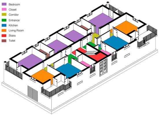
Figure 1.
Axonometric view of a typical residential building representative of the sample analysed.
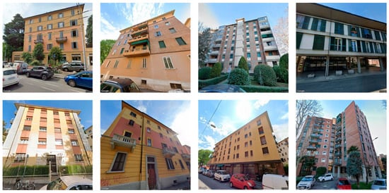
Figure 2.
Google street views of a subsample of the buildings under investigation.
2.2. State of the Art
2.2.1. Graph-Based Analysis for Spatial Layouts
Graph theory is instrumental in designing and analysing building layouts [3]. Graph-based approaches offer various methods and tools for generating architectural floor plan layouts [3,6] and analysing spatial configurations [3,7,8]. Researchers have proposed techniques to represent floor plans as graphs, effectively capturing spatial relationships and semantic information [9,10]. For instance, Lu et al. [3] proposed a workflow for the procedural generation of room relation graphs, leveraging vectorised floor plans to create corresponding organisational graphs for subsequent graph-based deep learning. Herthogs et al. [8] utilised justified plan graph analysis as a graph-based method to assess the generality and adaptability of building layouts quantitatively. Azizi et al. [9] represent floor plans as attributed graphs to capture geometric, semantic, and behavioural information. Zhang et al. [7] introduced an automated floor plan analysis system that extracts geographic information from floor plans and generates a weighted graph representation.
Keleş et al. [11] integrated graph theory with space syntax methodologies [12,13] to assess the accessibility of public buildings, utilising metrics such as integration, connectivity, and depth. Isaac et al. [14] utilised a graph-based representation to model building components and their relationships by integrating graph theory with Building Information Management (BIM) to uncover complex interdependencies within buildings. Similarly, Ernst et al. [15] applied a graph-based approach to optimise road lighting design, emphasising spatial elements and their interconnections. Cao et al. [16] developed an energy prediction model that transformed spatial layouts into graphs, which were then analysed using Graph Neural Networks (GNNs).
A graph represents a structure consisting of points, known as vertices, and the connections between them, referred to as edges [17]. As per Xie and Ding [6], an architectural floor plan can be depicted using dual graphs, where nodes correspond to rooms or spaces, and edges signify their connections. Each edge represents the adjacency relationship between the connected spaces [18]. Standard measures such as degree, closeness, betweenness, and eigenvector centrality were employed in graph-based analysis, in which critical insights into structural properties and hierarchies within spatial networks can be obtained [19]. Centrality measures reflect the morphological and topological characteristics of graphs by assessing a node’s importance based on its relationship with all other nodes in the graph [20,21]. Yang and Worboys [22] propose an automated approach for generating navigation graphs for indoor spaces to assess their connectivity. As per Bhattacharya et al. [23] the clustering coefficient of a graph offers insights into its connectivity.
2.2.2. Floor Plan Datasets
Recent research has emphasised the development and application of floor plan datasets for a range of architectural tasks. Kalervo et al. [24] presented CubiCasa5K, a dataset of 5000 annotated floor plan images, along with an improved multi-task convolutional neural network model for automated floor plan image analysis. Lu et al. (2021) [3] presented CubiGraph5K, a dataset of organisational graphs derived from vectorised architectural floor plan datasets derived from CubiCasa5K, designed to support graph-based deep learning. Goyal et al. [25] introduced BRIDGE, a large-scale public dataset comprising over 13,000 annotated floor plan images that support multiple tasks, including symbol spotting, caption and description generation, scene graph synthesis, and retrieval. Engelenburg et al. [26] developed the Modified Swiss Dwellings (MSDs) dataset, the first large-scale floor plan dataset featuring a substantial number of multi-apartment building layouts, which aims to address the scarcity of diverse and realistic floor plan data for architectural design applications.
Additionally, Wu et al. [27] developed RPLAN, a manually curated, large-scale dataset comprising 80,000 densely annotated floor plans from real residential buildings. RPLAN was utilised by Hu et al. [28] to train their Graph2Plan generative model. These datasets fulfil the demand for diverse and realistic floor plan data, enhancing the training and performance of ML models in architectural design and spatial analysis. For instance, House-GAN, a graph-constrained generative adversarial network designed to generate realistic and diverse house layouts while adhering to input architectural constraints, was trained on a dataset of 117,000 actual floor plan images [29].
3. Materials and Methods
3.1. Workflow Overview
This section presents the methodology followed to semi-automatically generate the graphs and topological models representing the floor plans’ spatial components and their interconnections.
The proposed workflow, outlined in Figure 3, comprises four different steps:
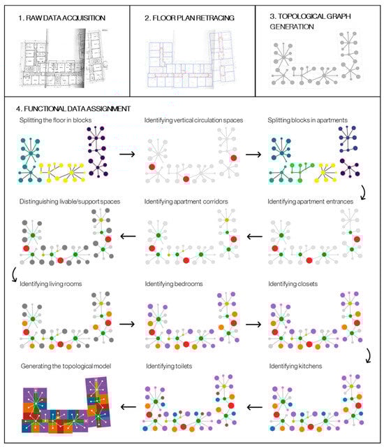
Figure 3.
Overview of the workflow for generating graphs and topological models of buildings’ floor plans.
- Raw data acquisition: the building’s typical floor plans are acquired in a raw format.
- Floor plan retracing: the spaces and the doors in the floor plans are manually retraced in a 3D modelling environment.
- Topological data generation: a 3D topological model mapping spaces and the data generation: a 3D topological model mapping spaces and their passage relationships through doors for each floor plan is generated thanks to a VPL algorithm.ir passage relationships through doors for each floor plan is generated thanks to a VPL algorithm.
- Functional data assignment: the occupancy types of the spaces in the floor plan are assigned through a procedure that leverages conditional data enrichment techniques based on the analysis of graph centrality metrics and morphological attributes of spaces.
3.2. Raw Data Acquisition
In this phase, raw data are acquired. These data consist of planimetric images of the typical floors from the analysed buildings, extracted from original drawings and technical reports associated with original building permits. This data source is particularly valuable, as it allows the accurate determination of floor layouts without the necessity of physically entering the buildings, a procedure that would be both time-consuming and invasive in terms of privacy given the residential nature of the structures.
The raw data of the buildings analysed result from archival research carried out at the Historical Archives of the Emilia Romagna Region (ParER). Specifically, the buildings investigated are blocks of flats built using public funds in the municipality of Bologna between 1945 and 1965. Contrary to the private buildings constructed during this period, for which few documents were required, the application for public funds had to be accompanied by a large number of official deeds and technical documents demonstrating the feasibility and regularity of the project. As a result, in addition to plans and sections, each building analysed was accompanied by a great deal of information not otherwise available, such as estimated metric calculations, structural plans, special specifications, and technical and photographic reports. For each building studied, the original drawings and all the documents considered most relevant for its complete definition were then digitally scanned. This led to the definition of the database containing all the raw floor plans used in the subsequent steps. Figure 4 shows typical floor plans of some buildings analysed characterised by various configurations.
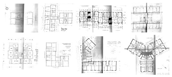
Figure 4.
Raw floor plans for a sample of the investigated buildings.
3.3. Floor Plan Retracing
In this workflow phase, the raw floor plans are transformed into a digital format using Rhino 3D, laying the groundwork for subsequent topological modelling and functional data prediction. The process involves three key steps:
- The initial step is to import the raw floor plan data into Rhino, ensuring that the original architectural drawings are available in a 3D modelling environment, where their geometry and scale can be manipulated.
- Once imported, each space within the floor plan is manually retraced by drawing closed polylines delineating the gross area of each space.
- In parallel with space retracing, door locations are defined by manually adding vertices at the centre of each door opening. By using these vertices, the following algorithms capture the connectivity between spaces.
Examples of retraced floor plans are depicted in Figure 5.
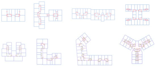
Figure 5.
Retraced floor plans for a sample of the buildings under investigation.
3.4. Topological Graph Generation
This step leverages a Grasshopper script, built upon the Topologic framework [30,31], to convert the manually retraced space curves and door vertices into a topological model and passage graph. The algorithm involves several sequential operations.
First, the retraced curves are scaled to the building’s real-world dimensions, ensuring that all subsequent analyses reflect accurate spatial measures. Second, the scaled curves are optimised by snapping them onto a 10 cm square grid. This adjustment helps align nearby vertices and edges, compensating for minor inaccuracies from the manual retracing process. Once optimised, the 2D curves are extruded into 3D, generating closed BRep surfaces. These BReps are subsequently transformed into Topologic Cells, which serve as the basic units for capturing spatial adjacencies, and the individual Topologic Cells are merged into a Topologic CellComplex. This model encapsulates all the adjacencies between different spaces, forming the backbone for the topological analysis. Dummy door geometries, designed with a fixed width of 80 cm and a height of 210 cm, are generated and projected onto the nearest surfaces of the Topologic model. The projected door geometries, processed as Topologic Apertures, are then added to the CellComplex, enriching it with information about the connectivity between spaces. Using the enriched CellComplex, the algorithm creates a Topologic Graph that maps all the passage relationships, representing how different spaces are interconnected through the doors, i.e., the floor plan layout. Finally, the resulting passage graph is exported in CSV format for further analysis, and the complete Topologic CellComplex is output as a BRep. Figure 6 illustrates the main results of this step.
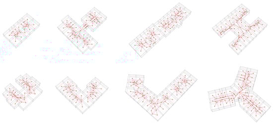
Figure 6.
Topologic Graph and CellComplex for a sample of the buildings under investigation.
3.5. Functional Data Assignment
In the final phase of the workflow, a Python 3.8.5 algorithm automatically assigns the function to each space according to 11 rulesets based on topological and geometric characteristics extracted from the passage graph. These rulesets, described below, were determined after iterative and careful observation of the floor plans analysed, which, as stated, belong to a set of buildings with similar function, age, location, and construction characteristics.
The functional data assignment process begins by importing the CSV representations of the graph into Python as both a NetworkX 3.1 graph [32] (to compute graph analytics and centrality metrics) and a Topologic Graph (to manage geometrical and shape attributes). Before applying the assignment rules, the algorithm extracts the connected components of each floor plan graph to analyse each one separately, each representing a “building block”, i.e., a part of the building with an independent passage layout from the other parts of the floor (Figure 7).
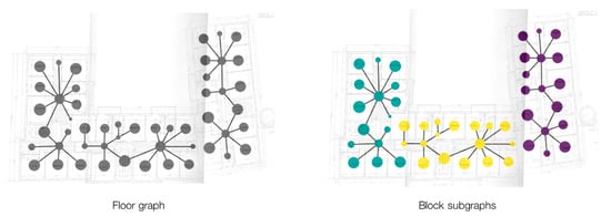
Figure 7.
A floor plan graph split into building block subgraphs. On the right, nodes are coloured by building block.
3.5.1. Ruleset 1: Identifying the Stairs via Uniform Component Decomposition Centrality
The first ruleset allows for the identification of the stairs, which are detected as the most central node in the building block graph. The algorithm introduces a new graph metric called Uniform Component Decomposition Centrality (UCDC) for this purpose. The key steps for its application are as follows:
- For every node in that building block graph, the node is temporarily removed, and any resulting isolated nodes in the graph are discarded.
- The modified graph is split into its connected subgraphs. For the removed node, the algorithm calculates the sizes (number of nodes) of the resulting subgraphs.
- The algorithm computes the standard deviation of the subgraphs’ sizes (in terms of number of nodes in the subgraph) to quantify how evenly the graph splits without the node.
- The standard deviation is then rescaled, and a negative logarithm is applied to produce a score, meaning that a lower standard deviation (i.e., more homogeneous component sizes) results in a higher UCDC score. This score is normalised and assigned to the node as its UCDC.
- Within each building block, the node with the highest score (i.e., the one whose removal yields the most balanced split) is identified as the staircase node, serving as the root of that building block (Figure 8).
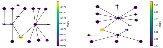 Figure 8. Block graphs after the detection of stairs (nodes coloured by UCDC). “None” nodes have unassigned functions at this step.
3.5.2. Ruleset 2: Detecting Elevators
After the staircase has been identified, the algorithm detects “elevator” nodes as those nodes with degree 1 connected to a “stairs” node (meaning their only neighbour is the staircase). Additionally, to be classified as an elevator, the space must have an area that is less than 50% of the staircase’s area. If a node is connected only to the staircase but exceeds 50% of the staircase area, it is instead classified as a “storage” space. This value was determined and tuned by visually examining the investigated dataset and iteratively testing the ruleset with different thresholds.
3.5.3. Ruleset 3: Apartment Graph Extraction and Entrance Identification
After the staircase and elevator nodes have been found, they are removed from the building block graph. The remaining connected components—each containing more than one node—are then isolated as individual subgraphs. These subgraphs represent the apartment graphs (Figure 9).
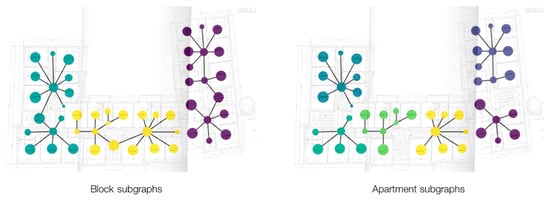
Figure 9.
Block graphs split into apartment subgraphs. On the left, nodes coloured by building block. On the right, nodes coloured by apartment.
The nodes directly connected to the removed staircase (in the original block graph) are designated as the apartment “entrances” within each apartment graph. From this step ahead, the analysis proceeds within the apartment graphs.
3.5.4. Ruleset 4: Corridor Assignment
In each apartment graph, corridors are identified after the entrance definition. In architectural layout, corridors are intended as the spatial elements that allow passage between spaces. In other words, spaces with this functionality allow two or more adjacent spaces to connect.
They are found by computing the minimum spanning tree of the apartment graph and marking all nodes with a degree greater than one as corridors. By virtue of their connectivity, these nodes are assumed to serve as transit spaces (see Figure 10).
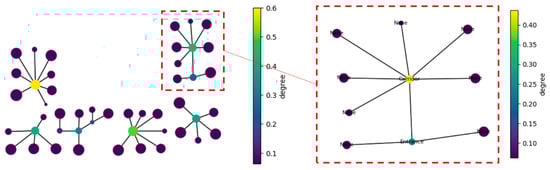
Figure 10.
Apartment graphs with nodes coloured by degree centrality. The nodes with degree centrality not null (i.e., the nodes that are not leaves) are set entrances or corridors. “None” nodes have unassigned functions at this step.
3.5.5. Ruleset 5: Distinguishing Corridors from Pass-Through Living Rooms
The preliminary corridor assignment rule (Rule 4) sometimes misclassifies some circulation spaces as corridors. While these spaces function as circulation areas, they also serve as living rooms. To identify these “pass-through living rooms”, three node-chain configurations have been developed to reclassify nodes based on their connectivity characteristics.
- Chain A: this configuration comprises nodes connected in the sequence “Entrance—Corridor—Corridor”. The central corridor is designated as a pass-through living room if its area is greater than that of the second corridor if the degree (number of connections) of the second corridor is higher than that of the central corridor, and if the degree of the central corridor is less than or equal to three.
- Chain B: this configuration comprises nodes connected in the sequence “Corridor—Corridor—None”, where “None” indicates that the node has not yet been classified. In this chain, the central corridor is reclassified as a pass-through living room if its area exceeds that of each adjacent node that is not classified as a corridor if the degree of the first corridor is greater than that of the central corridor, and if the degree of the central corridor is less than or equal to 3.
- Chain C: this configuration comprises nodes connected in the sequence “Entrance—Corridor—None”. Here, the corridor is classified as a pass-through living room if its area is larger than that of each adjacent non-corridor node and if its degree is less than or equal to 3.
Examples of Chain A, Chain B, and Chain C are depicted in Figure 11.
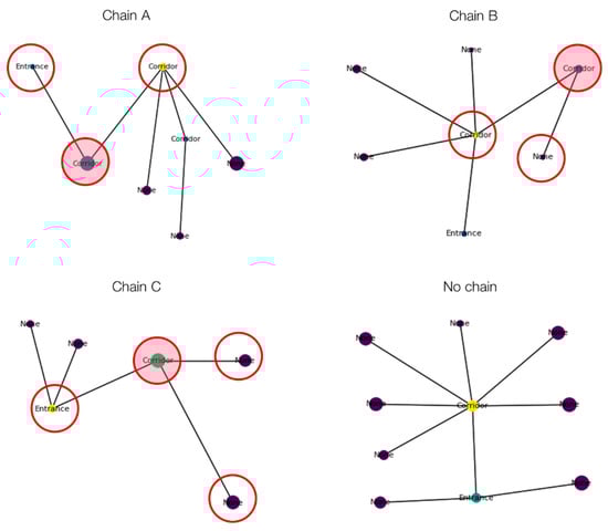
Figure 11.
Examples of Chain A, Chain B, and Chain C configurations in the analysed dataset. “None” nodes have unassigned functions at this step.
These chain-based rules enable the algorithm to correct misclassifications by reassigning nodes that, although they might serve as transitional spaces, function more like pass-through living rooms based on their relative size and connectivity.
3.5.6. Ruleset 6: Differentiating Liveable from Non-Liveable Spaces
After the entrances, corridors, and pass-through living rooms have been extracted from each apartment graph, the remaining nodes—those with lower-degree centrality—are analysed to distinguish between liveable spaces (e.g., bedrooms, living rooms) and non-liveable spaces (e.g., closets, bathrooms).
This classification strategy relies on the K-Means clustering method, an iterative, centroid-based clustering algorithm that partitions a dataset into similar groups based on the distance between their centroids [33].
Two approaches were tested to understand which centrality and dimensional features affect the clustering procedure.
- Approach A: Initially, each apartment’s unclassified nodes (i.e., those not already labelled as “corridor”, “entrance”, or “pass-through living room”) were clustered using K-Means with three clusters. The clustering used features that combined both the gross area and centrality metrics (i.e., betweenness, closeness, and degree centrality in the apartment graph). The clusters with the smallest average area were designated as “Supporting” spaces. The remaining clusters were classified as “Living” spaces. Moreover, if the cluster with a medium average area had a mean area below 65% of the cluster with the highest average area (a threshold derived from the ratio of the smallest single bedroom to the smallest double bedroom in Bologna according to local regulation), then even those nodes were reclassified as “Supporting”.
- Approach B: Then, due to the sensitivity issues associated with this approach (e.g., recurrent failures to correctly identify small single bedrooms as living spaces in apartments containing many large rooms), the algorithm was simplified to perform K-Means clustering using only the area attribute and reduce the number of clusters to 2.
Example results are provided in Figure 12.
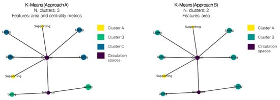
Figure 12.
K-Means algorithm applied to an apartment graph to classify living and supporting spaces.
3.5.7. Ruleset 7: Identifying the Living Room
This step identifies the living room between the nodes classified as “Living”.
Assuming that each apartment has only one living room, to determine which node among the “Living” spaces is the living room, the algorithm prioritises the following:
- Proximity to the entrance: the closer a node is to the designated entrance, the more likely it is to function as the living room.
- Connectivity (degree): nodes with a higher number of connections (i.e., a higher degree) are more central in the apartment’s circulation and thus are favoured.
- Size: a larger area increases the likelihood of the node serving as the living room.
The node that best meets these criteria is labelled the “Living Room”.
3.5.8. Ruleset 8: Classifying Bedrooms
Once the living room has been identified among the nodes previously classified as “Living”, all remaining nodes in that category are subsequently classified as bedrooms. Figure 13 outlines this and the previous steps.
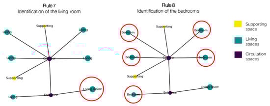
Figure 13.
Identification of the living room and of the bedrooms for an apartment graph.
3.5.9. Ruleset 9: Identifying Closets
Among the nodes designated as “Supporting” spaces, the algorithm identifies closets by selecting those nodes whose area is smaller than 30% of the average area of the rooms in the apartment. This threshold was determined empirically through iterative testing.
3.5.10. Ruleset 10: Kitchen Identification
Then, the kitchen is determined. The algorithm assumes that each apartment contains a single kitchen. The identification of kitchens proceeds as follows.
For smaller apartments (i.e., composed of a maximum of four nodes), it is hypothesised that the kitchen is integrated into the living room.
For apartments with more than four nodes, the algorithm first examines the leaf nodes (nodes with degree 1) in the minimum spanning tree of the apartment graph that are connected to a “Living Room”. These are initially set as candidates for the kitchen. For apartments that contain at least one “Supporting” node and more than one bedroom, the kitchen is determined by reclassifying the “Living” node (which was previously marked as a bedroom) that has the smallest area. The rationale here is that if the kitchen is relatively large, it should not be confused with a dining or living area.
3.5.11. Ruleset 11: Setting Toilets
Finally, the algorithm processes the remaining “Supporting” spaces to designate them as toilets.
The output consists of the apartment, block and floor graphs with nodes labelled with their function, as illustrated in Figure 14.
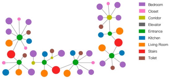
Figure 14.
Floor plan graph with labelled nodes at the end of the functional data prediction step.
3.6. Data Export
In the end, any error due to process inaccuracies is manually fixed. Then, after assigning the functional types to the nodes, the floor, block and apartment graphs are exported in JSON format as NetworkX and Topologic graphs with nodes containing the information reported in Table 1 and Table 2. Figure 15 shows the output graph of a floor plan with nodes coloured with relevant centrality scores.

Table 1.
Centrality metrics, calculated through NetworkX, added to the nodes in the graphs before the export.
Table 2.
Morphological and dimensional metrics, calculated topologically, added to the nodes in the graphs before the export.
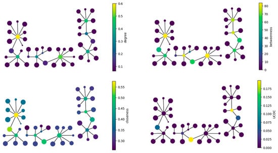
Figure 15.
Floor plan graph with nodes coloured by different types of centrality scores at the block level (degree, betweenness, closeness, and UCDC).
3.7. Sensitivity Analysis
After generating the dataset, to systematically assess which node features are most influential in distinguishing between occupancy types, a sensitivity analysis is conducted using a Random Forest (RF) classifier. This analysis is performed on node-level data extracted from the graphs, encompassing multiple spatial scales (i.e., floor, block, and apartment).
The node attributes are extracted and aggregated into a single data frame for each JSON file exported in the previous step. These nodes are characterised by the numerical properties provided in Table 1 and Table 2, including shape features (e.g., rectangularity, SV ratio, compactness, and gross area) and several network centrality measures (i.e., betweenness, closeness, degree, UCDC, and eigenvector centrality) computed at floor, block and apartment scales.
The target variable, representing the occupancy type of each node, is encoded using a label encoder. The dataset is then split into training and testing subsets using a 70/30 ratio. Missing values are handled via mean imputation to ensure completeness of the data. An RF classifier is therefore trained on the processed training data, using 1000 trees to ensure robustness. The choice of an RF is motivated by its intrinsic ability to provide measures of feature importance, making it particularly suitable for sensitivity analysis.
After training, the model’s feature important scores, which indicate the relative influence of each node feature in determining the occupancy type, are extracted and analysed.
4. Results
4.1. Dataset Description
The procedure described in the previous section was applied to 98 buildings, corresponding to 175 blocks and 392 apartments. A small subset of the graph dataset is depicted in Figure 16 and Figure 17.
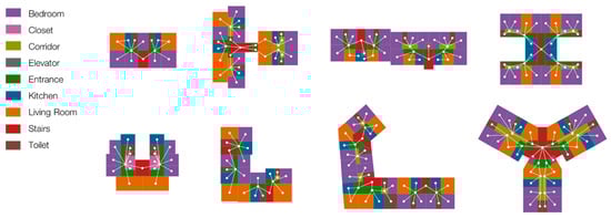
Figure 16.
Topologic models (with cells coloured by space occupancy type) for a sample of the buildings under investigation.
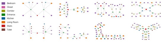
Figure 17.
NetworkX graphs (with nodes coloured by space occupancy type) for a sample of the buildings under investigation.
The following figures provide instead an overview of the study sample at the floor (Figure 18), block (Figure 19), and apartment level (Figure 20). Collectively, these distributions highlight a tendency toward smaller, simpler building configurations across the dataset, punctuated by some more complex structures.
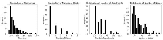
Figure 18.
Distribution of floor plans by total area, number of building blocks, apartments, and spaces.
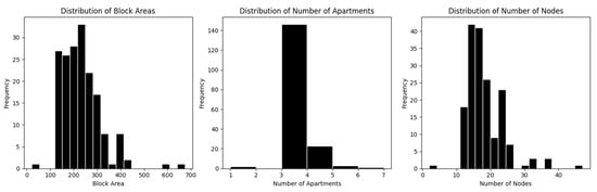
Figure 19.
Distribution of blocks by total area, apartment count, and number of spaces.
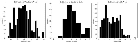
Figure 20.
Distribution of apartments by total area, number of spaces, and number of edges.
Floor Level Distribution: The distribution of floor areas demonstrates a right-skewed pattern, indicating that most floor plans have relatively small areas, while few exceed 1000 square metres. Regarding the block configuration, a single block per floor plan is the most common arrangement, whereas multi-block layouts occur less frequently. The number of apartments per floor plan is concentrated around lower values, with a noticeable peak between three and five apartments. Finally, the distribution of nodes, which represent spaces within the floor plan, follows a right-skewed trend. This suggests a general preference for simpler designs with fewer internal subdivisions.
Block Level Distribution: The figure below illustrates the distribution of blocks by total area, apartment count, and number of spaces. The data show that most block areas fall within 150 to 300 square metres. The data also indicate that blocks with three apartments are the most frequent, while those with four are the least frequent, suggesting the preference for three-unit configurations. Likewise, the distribution of spaces within each block is slightly skewed, with most blocks containing between 10 and 25 spaces.
Apartment Level Distribution: Apartment areas vary between 50 and 160 square metres, with most apartments within 90 to 110 square metres. The number of nodes, which represents the number of spaces per apartment, ranges from 2 to 30, with 7 being the most frequent.
4.2. Dataset Analysis
Figure 21 and Figure 22 provide a summary of the distribution of the primary functions within the study sample.
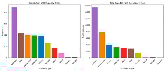
Figure 21.
Distribution of functions in the dataset (by total count and area).
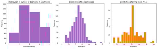
Figure 22.
Distribution of bedrooms and living room (by total count and area).
Figure 21 provides information about the distributions of the node functions in the dataset, with the chart on the left illustrating the number of nodes and the chart on the right showing the total gross area of the spaces. Overall, these charts indicate that bedrooms are both the most numerous and occupy the greatest total area in this dataset, as expected, with living rooms also occupying a consistently substantial area. The number of living rooms, toilets and kitchens is almost equal to the number of apartments analysed, suggesting that nearly every apartment includes one toilet and one kitchen.
Figure 22 shows the apartments’ distribution of bedrooms and living rooms, indicating that most apartments in the dataset have two or three bedrooms. The bedroom areas typically range from 10 to 25 sqm of gross area, with a peak at approximately 18 sqm, while living room areas generally range from 14 to 29 sqm, peaking at around 21 sqm. Few outliers are observed at either the smaller or larger end of these distributions.
Figure 23 depicts the top 10 node features, ranked based on their importance, in a vertical bar plot. From this bar chart, it is clear that shape and size metrics (particularly SV ratio and gross area) emerge as the most influential features in the classification task, reflecting that a node’s geometric properties (e.g., volume/area ratio and overall size) are highly predictive of its occupancy type. In addition, in addition to these shape descriptors, centrality measures, notably closeness and betweenness at the building scale, also appear among the top features, indicating that how a space is integrated within the larger building network plays a meaningful role. The presence of apartment-scale centralities in the top 10 further underscores that node connectivity and position at the apartment level can still inform the classification, albeit to a lesser extent than the floor-level measures and the geometric properties.
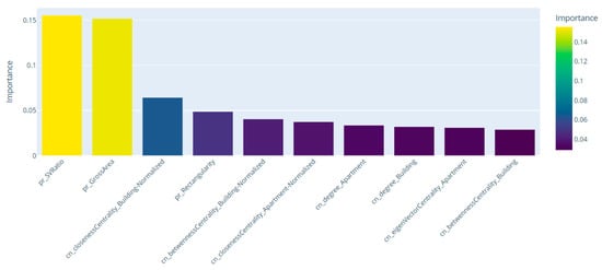
Figure 23.
Results of the sensitivity analysis on node features, highlighting the relative importance of each attribute in the classification model.
Figure 24 presents box plots comparing the top four node features (SV ratio, gross area, closeness centrality, and rectangularity) across the dataset’s occupancy types. Bedrooms and living rooms generally exhibit larger areas, whereas bathrooms, corridors, and stairs are notably smaller. The SV ratio varies among occupancy types: corridors, for example, may show higher medians or wider spreads, while bedrooms and living rooms tend to be more compact. Concerning closeness centrality, corridors, stairs, and entrances exhibit higher values due to their role as spatial connectors, whereas bathrooms, bedrooms, and storage areas are more peripheral, exhibiting lower centrality. Living rooms often have intermediate values, since many of them serve as pass-through spaces. Finally, in terms of rectangularity, bedrooms and living rooms frequently display higher rectangularity—indicating they are closer to a square shape—while stairs and corridors can be more irregular, often enclosed in elongated rectangular layouts.
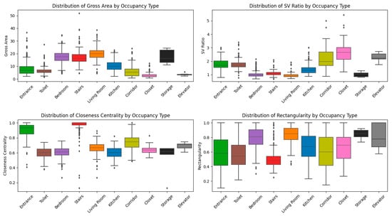
Figure 24.
Distribution of the top 4 node features across the dataset.
5. Discussion
5.1. Evaluation of Process Accuracy
With regard to the process of functional data prediction, this application iteratively enabled the understanding of the previously described rules for the attribution of functional data. Not all rules yielded positive results in every case study. Below, the accuracy of the main steps of the process application is evaluated with respect to the considered sample.
5.1.1. Evaluation of Rulesets 1 and 2: Stairs and Elevators
For the definition of Ruleset 1, various centrality measures were tested to detect the stairs node automatically; however, the most commonly used ones did not yield satisfactory results. As previously reported, a new metric for analysing node centrality was developed to address this: UCDC. In summary, this metric identifies the node that, if removed from the graph, divides it into components of as homogeneous a size as possible. UCDC allowed us to identify the staircase node with a success rate of approximately 94%, failing in only 12 building blocks where the node with the highest UCDC did not correspond to a staircase. As expected, this metric fails in blocks with less symmetrical architectural layout. More specifically, UCDC succeeded in 94.4% of cases, while the node with the highest closeness centrality corresponded to the staircase in 74% of cases. In contrast, betweenness, eigenvector, and degree centrality succeeded in only 23%, 8%, and 3% of cases, respectively.
Ruleset 2 was successful in all cases. It was discovered that only 14 blocks have an elevator, corresponding to 8% of the total number of building blocks, which also belong to higher buildings.
5.1.2. Evaluation of Rulesets 3, 4 and 5: Entrances, Corridors and Pass-Through Living Rooms
While the application of Ruleset 3 was successful in all cases, as anticipated, Ruleset 4 produced several inaccuracies because it classified spaces that are actually living rooms as corridors. In fact, this is not a flaw in the method itself but rather a reflection of its underlying assumptions. Indeed, if a living room permits passage between an entrance/corridor and other spaces—such as the kitchen or, in some cases, a bedroom—then, topologically, it facilitates transit between two areas; in other words, it is a circulation space and can be considered a corridor. The analysed dataset found that many apartments exhibit a spatial configuration corresponding to the description above. Specifically, in 162 apartments (approximately 42%), configurations corresponding to Chain A, Chain B, and Chain C were observed.
More specifically, the following observations were made:
- Chain A was observed in 23 apartments (6.0% of the total). This configuration occurs when a pass-through living room is situated between two corridors, following the specified conditions.
- Chain B was found in 28 apartments (7.3%). In this case, the pass-through living room appears between two corridors, with one of them leading to a dead end.
- Chain C was the most common, appearing in 113 apartments (29.4%). Here, the pass-through living room is formed between the entrance and a single corridor, which ends in a dead end.
5.1.3. Evaluation of Ruleset 6: Living vs. Supporting Spaces
Ruleset 6 is perhaps the least accurate method, leaving room for further improvement. In this task, the goal was to distinguish which leaf nodes in the minimum spanning tree of apartment graphs represent supporting spaces and which represent living spaces.
Two approaches were tested: one applying K-Means clustering using both dimensional and centrality metrics and another using only dimensional metrics. The second approach demonstrated that the clustering algorithm was insensitive to the architectural significance of nodes in terms of centrality, indicating that the primary distinguishing feature is the gross area. In similar buildings, these types of spaces always exhibit the same topological centrality, as they are typically leaf nodes connected to only one space.
Moreover, there were certain edge cases where K-Means failed. For example, the algorithm failed when an apartment had one room significantly larger than the other small bedrooms or living rooms were erroneously classified as supporting spaces instead of living spaces. Similarly, when there was a closet much smaller than the bathrooms, the closet was classified as supporting while the bathrooms were classified as living. This observation led to the decision to simplify the process using K-Means clustering, which considers only the area attribute and disregards centrality metrics.
The simplified approach failed in 15% of cases (59 apartments), showing a very slight improvement over the first approach, which failed in 16% of cases. This similarity in results demonstrates that centrality metrics do not influence distinguishing between “Living” and “Supporting” spaces.
An additional rule was applied to correct these inaccuracies: all nodes with a gross area greater than 10 were classified as “Living”, while the others were classified as “Supporting”. Among the 59 apartments that previously failed, this strategy was successful in 56 cases (approximately 95%). For the remaining three buildings, the misclassified nodes were manually adjusted.
5.1.4. Evaluation of Ruleset 7, 8, 9, 10 and 11: Living Rooms, Bedrooms, Kitchens, Toilets, and Closets
These final steps are evaluated together because, given how the rules are defined, the failure of one ruleset almost always leads to the failure of subsequent ones.
After the execution of these steps, all graphs were manually corrected by cross-checking the original floor plans of the buildings. At the end of the process, it was found that only 320 out of 3147 nodes (approximately 10.2%) were misclassified.
Among the misclassified nodes (i.e., false negatives), 124 bedrooms and 125 kitchens were erroneously assigned to other functions, compared to 18 closets, 29 toilets, and 22 living rooms.
The main errors are due to some nodes being confused with other topologically and dimensionally very similar nodes. The primary errors are as follows:
- Single bedroom vs. kitchen: These are often confused when the kitchen is directly connected to the corridor (entrance) and is not connected to other spaces. Considering that Italian regulations (Istruzioni Ministeriali 20 Giugno 1896) stipulated a minimum of 9 square metres for both kitchens and single bedrooms, this error is understandable. In such cases, the approach cannot yield better results.
- Living rooms vs. large bedrooms: The same consideration applies. Established Italian regulations require that living rooms and double bedrooms have a net area greater than 14 square metres. When identified topologically in terms of centrality, living rooms can be confused with bedrooms. Again, the algorithm cannot do much in these cases.
- Small kitchen vs. toilets: A small kitchen can be confused with toilets when the toilets are larger, for similar reasons.
- Small toilets vs. closets: Another recurring error occurs when bathrooms are smaller than closets. Indeed, the process assumes that closets are the nodes with the smallest area among those classified as supporting spaces.
5.2. Limitations and Future Studies
This study offers a graph-based approach to generating a residential building floor plan dataset and assigning node functions through conditional data enrichment techniques. Although good results were achieved on the presented dataset, several limitations should be acknowledged.
First, this study is built on a relatively small dataset of floor plans, which opens the door for more future work by investigating the offered methodology’s applicability on larger datasets. Moreover, the proposed method is applied to residential buildings, which limits the generalisation of methodology to buildings with other functions, as well as more complex and large-scale buildings, including commercial or institutional buildings. Furthermore, this study is context-sensitive, since it considers buildings from Italy built in a specific period according to a spread of architectural practice in the Italian territory between the 1940s and 1960s. This aspect, which limits the generalisation of the approach to other regional contexts, pushes the interest of extending the study to different contexts to validate its methodology and make logical comparisons of different residential typologies.
From the methodological point of view, this study can be extended to include community detection methods for investigating zones and communities within layouts, further improving specific steps of the functional data enrichment process (e.g., stairs detection). In addition, while the approach is computationally efficient for small-scale layouts, its scalability to larger or highly irregular buildings may introduce processing challenges.
Future work could address these limitations by expanding the dataset to include more diverse building types and incorporating additional spatial metrics alongside graph-based features.
6. Conclusions
This study introduced an automated approach to generating a dataset for residential buildings using a topological graph-based methodology, which addresses a gap in conventional architectural datasets that primarily focus on only geometric attributes. It proposes an automated methodology for encoding spatial relationships, adjacency, and connectivity between spaces within residential layouts, extending centrality measures to define functional roles of spaces within residential layouts. By analysing the topological importance of spaces within the spatial network, this research explored how graph-based metrics can predict the function of spaces without prior labelling.
The dataset generated in this study provides a foundation for researchers to explore graph-based analysis, centrality-driven design automation, and functional prediction in architectural layouts. Additionally, it enables the automatic classification of spaces based on their graph centrality values, facilitating future integration of graph-based analysis with ML techniques.
The presented work will be further developed in the future with three key objectives. First, the dataset of floor plan layouts will be extended by integrating the proposed methodology with supervised ML techniques for node function prediction (such as RFs, ANNs, and GNNs). Using the dataset generated in this study, future work will assess which of these ML models perform best and identify the most relevant features to streamline the data collection and analysis process. Second, future work is aimed at exploring unsupervised ML techniques, such as K-Means and DBSCAN, for clustering graphs based on dimensional, geometric, and spatial connectivity characteristics. This clustering will help categorise buildings into architectural types for urban analysis so that, after the clustering, by employing methods such as the nearest-neighbour chain algorithm, it will be possible to associate new buildings (not included in the dataset) with these types, enabling fast urban-scale data collection and analyses. Finally, the third goal will be to integrate spatial data with additional contextual information, such as construction features and visual characteristics of the buildings. Integrating these data—which are currently being acquired through in situ surveys, the examine of original building permits, and computer vision techniques—into topological models will allow for a more comprehensive classification of buildings into “digital archetypes” (on the basis of construction, functional, spatial, and performance characteristics), ultimately supporting data-driven urban policymaking.
Author Contributions
Conceptualization, A.M.; methodology, A.M. and W.J.; software, A.M. and W.J.; validation, D.H.A.-H., L.S. and W.J.; formal analysis, A.M.; investigation, A.M.; resources, L.S.; data curation, A.M. and D.H.A.-H.; writing—original draft preparation, A.M. and D.H.A.-H.; writing—review and editing, L.S. and W.J.; visualisation, A.M.; supervision, W.J. All authors have read and agreed to the published version of the manuscript.
Funding
This research received no external funding.
Data Availability Statement
The datasets presented in this article are not readily available because the data are part of an ongoing study. Requests to access the datasets should be directed to angelo.massafra@unibo.it.
Conflicts of Interest
The authors declare no conflicts of interest.
Abbreviations
The following abbreviations are used in this manuscript:
| AECO | Architecture, Engineering, Construction, and Operations. |
| ANN | Artificial neural network. |
| BIM | Building information modelling. |
| GIS | Geographic Information System. |
| GNN | Graph Neural Network. |
| ML | Machine learning. |
| RF | Random Forest. |
| UCDC | Uniform component decomposition centrality. |
| VPL | Visual Programming Language. |
References
- Italian National Institute of Statistics (ISTAT). Population and Housing Census. 2011. Available online: http://dati-censimentopopolazione.istat.it/Index.aspx (accessed on 13 March 2025).
- Lehtola, V.V.; Koeva, M.; Elberink, S.O.; Raposo, P.; Virtanen, J.-P.; Vahdatikhaki, F.; Borsci, S. Digital Twin of a City: Review of Technology Serving City Needs. Int. J. Appl. Earth Obs. Geoinf. 2022, 114, 102915. [Google Scholar] [CrossRef]
- Lu, Y.; Tian, R.; Li, A.; Wang, X.; Garcia del Castillo Lopez, J.L. CUBIGRAPH5K: Organizational Graph Generation for Structured Architectural Floor Plan Dataset. In Proceedings of the 26th International Conference of the Association for Computer—Aided Architectural Design Research in Asia (CAADRIA 2021), Hong Kong, China, 29 March–1 April 2021; Volume 1, pp. 81–90. [Google Scholar]
- Parenti, G. Una Esperienza Di Programmazione Settoriale Nell’edilizia: L’ina-Casa; Giuffrè: Roma, Italy, 1967. [Google Scholar]
- Ministero dei Lavori Pubblici. Legge 2 Luglio 1949, n. 408: Disposizioni per l’incremento Delle Costruzioni Edilizie; Ministero dei Lavori Pubblici: Rome, Italy, 1949. [Google Scholar]
- Xie, X.; Ding, W. An Interactive Approach for Generating Spatial Architecture Layout Based on Graph Theory. Front. Archit. Res. 2023, 12, 630–650. [Google Scholar] [CrossRef]
- Zhang, X.; Wong, A.K.-S.; Lea, C.-T. Automatic Floor Plan Analysis for Adaptive Indoor Wi-Fi Positioning System. In Proceedings of the 2016 International Conference on Computational Science and Computational Intelligence (CSCI), Las Vegas, NV, USA, 15–17 December 2016; pp. 869–874. [Google Scholar]
- Herthogs, P.; De Temmerman, N.; De Weerdt, Y. Assessing the Generality and Adaptability of Building Layouts Using Justified Plan Graphs and Weighted Graphs: A Proof of Concept. In Proceedings of the Central Europe towards Sustainable Building 2013: Sustainable Refurbishment of Existing Building Stock, Prague, Czech Republic, 26–28 June 2013. [Google Scholar]
- Azizi, V.; Usman, M.; Zhou, H.; Faloutsos, P.; Kapadia, M. Graph-Based Generative Representation Learning of Semantically and Behaviorally Augmented Floorplans. Vis. Comput. 2022, 38, 2785–2800. [Google Scholar] [CrossRef]
- De Las Heras, L.-P.; Terrades, O.R.; Llados, J. Attributed Graph Grammar for Floor Plan Analysis. In Proceedings of the 2015 13th International Conference on Document Analysis and Recognition (ICDAR), Tunis, Tunisia, 23–26 August 2015; pp. 726–730. [Google Scholar]
- Keleş, B.N.; Takva, Ç.; Çakıcı, F.Z. Accessibility Analysis of Public Buildings with Graph Theory and the Space Syntax Method: Government Houses. J. Asian Archit. Build. Eng. 2025, 24, 199–213. [Google Scholar] [CrossRef]
- Hillier, B. A Theory of the City as Object: Or, How Spatial Laws Mediate the Social Construction of Urban Space. Urban Des. Int. 2001, 6, 153–179. [Google Scholar] [CrossRef]
- Hillier, B. Space Is the Machine: A Configurational Theory of Architecture; Cambridge University Press: Cambridge, UK, 1996. [Google Scholar]
- Isaac, S.; Sadeghpour, F.; Navon, R. Analyzing Building Information Using Graph Theory. In Proceedings of the 30th ISARC, Montreal, QC, Canada, 11–15 August 2013. [Google Scholar]
- Ernst, S.; Łabuz, M.; Środa, K.; Kotulski, L. Graph-Based Spatial Data Processing and Analysis for More Efficient Road Lighting Design. Sustainability 2018, 10, 3850. [Google Scholar] [CrossRef]
- Cao, J.; Zhang, H.; Savov, A.; Hall, D.; Dillenburger, B. Energy-Aware Design: Predicting Building Performance from Layout Graphs. In Proceedings of the Energy-Aware Design: Predicting Building Performance from Layout Graphs, Rhodes, Greece, 24–26 July 2022. [Google Scholar]
- Wilson, R.J. Introduction to Graph Theory, 4th ed.; Longman Group Ltd.: Harlow, UK, 1996. [Google Scholar]
- Wong, S.S.Y.; Chan, K.C.C. EvoArch: An Evolutionary Algorithm for Architectural Layout Design. Comput. -Aided Des. 2009, 41, 649–667. [Google Scholar] [CrossRef]
- Valente, T.W.; Coronges, K.; Lakon, C.; Costenbader, E. How Correlated Are Network Centrality Measures? Connections 2008, 28, 16–26. [Google Scholar] [PubMed]
- Werner, C.; Loidl, M. Betweenness Centrality in Spatial Networks: A Spatially Normalised Approach (Short Paper). GIScience 2023, 277, 83. [Google Scholar] [CrossRef]
- Wurzer, G.; Lorenz, W.E. SpaceBook: A Case Study of Social Network Analysis in Adjacency Graphs. In Complexity & Simplicity: Proceedings of the 34th eCAADe Conference, Oulu, Finland, 24–26 August 2016; Herneoja, A., Österlund, T., Markkanen, P., Eds.; TU Wien: Vienna, Austria, 2016; Volume 2, pp. 229–238. [Google Scholar]
- Yang, L.; Worboys, M. Generation of Navigation Graphs for Indoor Space. Int. J. Geogr. Inf. Sci. 2015, 29, 1737–1756. [Google Scholar] [CrossRef]
- Bhattacharya, S.; Sinha, S.; Dey, P.; Saha, A.; Chowdhury, C.; Roy, S. Online Social-Network Sensing Models. In Computational Intelligence Applications for Text and Sentiment Data Analysis; Elsevier: Amsterdam, The Netherlands, 2023; pp. 113–140. [Google Scholar] [CrossRef]
- Kalervo, A.; Ylioinas, J.; Häikiö, M.; Karhu, A.; Kannala, J. CubiCasa5K: A Dataset and an Improved Multi-Task Model for Floorplan Image Analysis. In Image Analysis; Felsberg, M., Forssén, P.-E., Sintorn, I.-M., Unger, J., Eds.; Lecture Notes in Computer Science; Springer International Publishing: Cham, Switzerland, 2019; Volume 11482, pp. 28–40. [Google Scholar] [CrossRef]
- Goyal, S.; Mistry, V.; Chattopadhyay, C.; Bhatnagar, G. BRIDGE: Building Plan Repository for Image Description Generation, and Evaluation. In Proceedings of the 2019 International Conference on Document Analysis and Recognition (ICDAR), Sydney, Australia, 20–25 September 2019; pp. 1071–1076. [Google Scholar]
- van Engelenburg, C.; Mostafavi, F.; Kuhn, E.; Jeon, Y.; Franzen, M.; Standfest, M.; van Gemert, J.; Khademi, S. MSD: A Benchmark Dataset for Floor Plan Generation of Building Complexes. arXiv 2024, arXiv:2407.10121. [Google Scholar] [CrossRef]
- Wu, W.; Fu, X.-M.; Tang, R.; Wang, Y.; Qi, Y.-H.; Liu, L. Data-Driven Interior Plan Generation for Residential Buildings. ACM Trans. Graph. 2019, 38, 1–12. [Google Scholar] [CrossRef]
- Hu, R.; Huang, Z.; Tang, Y.; Van Kaick, O.; Zhang, H.; Huang, H. Graph2Plan: Learning Floorplan Generation from Layout Graphs. ACM Trans. Graph. 2020, 39, 4. [Google Scholar] [CrossRef]
- Nauata, N.; Chang, K.-H.; Cheng, C.-Y.; Mori, G.; Furukawa, Y. House-GAN: Relational Generative Adversarial Networks for Graph-Constrained House Layout Generation. arXiv 2020, arXiv:2003.06988. [Google Scholar] [CrossRef]
- Jabi, W.; Chatzivasileiadi, A. Topologic: Exploring Spatial Reasoning Through Geometry, Topology, and Semantics; Advances in Science, Technology & Innovation; Springer: Cham, Switzerland, 2021. [Google Scholar]
- Jabi, W. Topologicpy, Version 0.8.15; 2024. Available online: https://zenodo.org/records/11555173 (accessed on 10 April 2025).
- NetworkX—NetworkX Documentation. Available online: https://networkx.org/ (accessed on 13 March 2025).
- MacQueen, J.B. Some Methods for Classification and Analysis of Multivariate Observations. In Proceedings of the Fifth Berkeley Symposium on Mathematical Statistics and Probability, Volume 1: Statistics; Le Cam, L.M., Neyman, J., Eds.; University of California Press: Berkeley, CA, USA, 1967; pp. 281–297. [Google Scholar]
- Crucitti, P.; Latora, V.; Porta, S. Centrality Measures in Spatial Networks of Urban Streets. Phys. Rev. E 2006, 73, 036125. [Google Scholar] [CrossRef] [PubMed]
- Perez, C.; Germon, R. Graph Creation and Analysis for Linking Actors: Application to Social Data. In Automating Open Source Intelligence: Algorithms for OSINT; Layton, R., Watters, P.A., Eds.; Elsevier: Amsterdam, The Netherlands, 2016; pp. 103–129. [Google Scholar]
- Golbeck, J. Nodes, Edges, and Network Measures. In Analyzing the Social Web; Elsevier: Amsterdam, The Netherlands, 2013; pp. 9–23. [Google Scholar] [CrossRef]
Disclaimer/Publisher’s Note: The statements, opinions and data contained in all publications are solely those of the individual author(s) and contributor(s) and not of MDPI and/or the editor(s). MDPI and/or the editor(s) disclaim responsibility for any injury to people or property resulting from any ideas, methods, instructions or products referred to in the content. |
© 2025 by the authors. Licensee MDPI, Basel, Switzerland. This article is an open access article distributed under the terms and conditions of the Creative Commons Attribution (CC BY) license (https://creativecommons.org/licenses/by/4.0/).