


Automatic Scan-to-BIM—The Impact of Semantic Segmentation Accuracy


Abstract
1. Introduction
1.1. Background
1.1.1. Semantic Segmentation
1.1.2. Wall Reconstruction
2. Materials and Methods
2.1. Dataset Preparation
2.2. Semantic Segmentation
2.2.1. Selection of Algorithms
2.2.2. Training
2.2.3. Evaluation
2.3. Wall Reconstruction
2.3.1. Wall Mask
2.3.2. Individual Wall Detection
2.3.3. Extracting Measurements
2.3.4. Reconstruction
2.3.5. Accuracy Assessment

3. Results
4. Discussion
5. Conclusions
Author Contributions
Funding
Data Availability Statement
Conflicts of Interest
Abbreviations
| BIM | Building Information Model/Modelling |
| AEC | Architecture, Engineering, and Construction |
| NIST | National Institute of Standards and Technology |
| RGBD | Red Green Blue Depth |
| RANSAC | Random Sampling Consensus |
| SIFT | Scale Invariant Feature Transform |
| PTV1 | Point Transformer Version 1 |
| PTV3 | Point Transformer Version 3 |
| KNN | K-Nearest Neighbour |
| S3DIS | Stanford 3D Indoor Scene Dataset |
| SOTA | State-of-the-art |
| CNN | Convolutional Neural Network |
| FPS | Farthest Point Sampling |
| MLP | Multi-Layer Perceptron |
| EPE | Explicit Positional Encoding |
| BN | Batch Normalization |
| ReLU | Rectified Linear Unit |
| cRSE | Contextual Relative Signal Encoding |
| RPE | Relative Positional Encoding |
| oAcc | Overall Accuracy |
| mAcc | Mean Class-wise Accuracy |
| mIoU | Mean Intersection Over Union |
| AABB | Axis-Aligned Bounding Box |
| IFC | Industry Foundation Class |
References
- Eastman, C. BIM Handbook: A Guide to Building Information Modeling for Owners, Managers, Designers, Engineers and Contractors; John Wiley & Sons: Hoboken, NJ, USA, 2011. [Google Scholar]
- Adekunle, S.A.; Aigbavboa, C.; Ejohwomu, O.A. SCAN TO BIM: A systematic literature review network analysis. IOP Conf. Ser. Mater. Sci. Eng. 2022, 1218, 012057. [Google Scholar] [CrossRef]
- Nwodo, M.N.; Anumba, C.J. A review of life cycle assessment of buildings using a systematic approach. Build. Environ. 2019, 162, 106290. [Google Scholar] [CrossRef]
- Pətrəucean, V.; Armeni, I.; Nahangi, M.; Yeung, J.; Brilakis, I.; Haas, C. State of research in automatic as-built modelling. Adv. Eng. Inform. 2015, 29, 162–171. [Google Scholar] [CrossRef]
- Gourguechon, C.; MacHer, H.; Landes, T. Automation of As-Built Bim Creation from Point Cloud: An Overview of Research Works Focused on Indoor Environment. Int. Arch. Photogramm. Remote Sens. Spat. Inf. Sci. 2022, 43, 193–200. [Google Scholar] [CrossRef]
- Borruso, G.; Huang, W.; Balletto, G.; Banfi, F.; Mura, M. Procedural Point Cloud Modelling in Scan-to-BIM and Scan-vs-BIM Applications: A Review. ISPRS Int. J. Geo-Inf. 2023, 12, 260. [Google Scholar] [CrossRef]
- Chmelar, P.; Rejfek, L.; Nguyen, T.N.; Ha, D.H. Advanced Methods for Point Cloud Processing and Simplification. Appl. Sci. 2020, 10, 3340. [Google Scholar] [CrossRef]
- Zhang, J.; Zhao, X.; Chen, Z.; Lu, Z. A Review of Deep Learning-Based Semantic Segmentation for Point Cloud. IEEE Access 2019, 7, 179118–179133. [Google Scholar] [CrossRef]
- Wang, Y.; Sun, Y.; Liu, Z.; Sarma, S.E.; Bronstein, M.M.; Solomon, J.M. Dynamic graph CNN for learning on point clouds. ACM Trans. Graph. 2019, 38, 146. [Google Scholar] [CrossRef]
- Zhao, H.; Jiang, L.; Fu, C.W.; Jia, J. Pointweb: Enhancing local neighborhood features for point cloud processing. In Proceedings of the IEEE/CVF Conference on Computer Vision and Pattern Recognition, Long Beach, CA, USA, 15–20 June 2019; pp. 5560–5568. [Google Scholar]
- Park, C.; Jeong, Y.; Cho, M.; Park, J. Fast Point Transformer. In Proceedings of the IEEE/CVF Conference on Computer Vision and Pattern Recognition, New Orleans, LA, USA, 18–24 June 2022; pp. 16928–16937. [Google Scholar]
- Qi, C.R.; Su, H.; Mo, K.; Guibas, L.J. PointNet: Deep learning on point sets for 3D classification and segmentation. In Proceedings of the 30th IEEE Conference on Computer Vision and Pattern Recognition, CVPR 2017, Honolulu, HI, USA, 21–26 July 2017; pp. 77–85. [Google Scholar]
- Engelmann, F.; Kontogianni, T.; Schult, J.; Leibe, B. Know What Your Neighbors Do: 3D Semantic Segmentation of Point Clouds; Lecture Notes in Computer Science (Including Subseries Lecture Notes in Artificial Intelligence and Lecture Notes in Bioinformatics); Springer: Berlin/Heidelberg, Germany, 2019; pp. 395–409. [Google Scholar]
- Wang, L.; Huang, Y.; Hou, Y.; Zhang, S.; Shan, J. Graph attention convolution for point cloud semantic segmentation. In Proceedings of the IEEE/CVF Conference on Computer Vision and Pattern Recognition, Long Beach, CA, USA, 15–20 June 2019; pp. 10288–10297. [Google Scholar]
- Wu, X.; Lao, Y.; Jiang, L.; Liu, X.; Zhao, H. Point Transformer V2: Grouped Vector Attention and Partition-based Pooling. Adv. Neural Inf. Process. Syst. 2022, 35, 33330–33342. [Google Scholar]
- Camuffo, E.; Michieli, U.; Milani, S. Learning from Mistakes: Self-Regularizing Hierarchical Representations in Point Cloud Semantic Segmentation. IEEE Trans. Multimed. 2023, 27, 978–989. [Google Scholar] [CrossRef]
- Lai, K.; Fox, D. Object Recognition in 3D Point Clouds Using Web Data and Domain Adaptation. Int. J. Robot. Res. 2010, 29, 1019–1037. [Google Scholar] [CrossRef]
- Lai, K.; Bo, L.; Ren, X.; Fox, D. A large-scale hierarchical multi-view RGB-D object dataset. In Proceedings of the IEEE International Conference on Robotics and Automation, Shanghai, China, 9–13 May 2011; pp. 1817–1824. [Google Scholar] [CrossRef]
- Quigley, M.; Batra, S.; Gould, S.; Klingbeil, E.; Le, Q.; Wellman, A.; Ng, A.Y. High-accuracy 3D sensing for mobile manipulation: Improving object detection and door opening. In Proceedings of the IEEE International Conference on Robotics and Automation, Kobe, Japan, 12–17 May 2009; pp. 2816–2822. [Google Scholar] [CrossRef]
- Shao, T.; Xu, W.; Zhou, K.; Wang, J.; Li, D.; Guo, B. An Interactive Approach to Semantic Modeling of Indoor Scenes with an RGBD Camera. ACM Trans. Graph. 2012, 31, 136. [Google Scholar] [CrossRef]
- Hedau, V.; Hoiem, D.; Forsyth, D. Thinking Inside the Box: Using Appearance Models and Context Based on Room Geometry. In Proceedings of the 11th European Conference on Computer Vision, Heraklion, Greece, 5–11 September 2010; Volume 6316, pp. 224–237. [Google Scholar] [CrossRef]
- Silberman, N.; Fergus, R. Indoor scene segmentation using a structured light sensor. In Proceedings of the IEEE International Conference on Computer Vision Workshops, Barcelona, Spain, 6–13 November 2011; pp. 601–608. [Google Scholar] [CrossRef]
- Nan, L.; Xie, K.; Sharf, A. A search-classify approach for cluttered indoor scene understanding. ACM Trans. Graph. 2012, 31, 137. [Google Scholar] [CrossRef]
- Xiong, X.; Huber, D. Using context to create semantic 3D models of indoor environments. In Proceedings of the British Machine Vision Conference, BMVC 2010, Aberystwyth, UK, 31 August–3 September 2010. [Google Scholar] [CrossRef]
- Galleguillos, C.; Rabinovich, A.; Belongie, S. Object categorization using co-occurrence, location and appearance. In Proceedings of the 26th IEEE Conference on Computer Vision and Pattern Recognition, CVPR, Anchorage, AK, USA, 23–28 June 2008. [Google Scholar] [CrossRef]
- Vosselman, G.; Gorte, B.G.H.; Sithole, G.; Rabbani, T. Recognising structure in laser scanning point clouds. Int. Arch. Photogramm. Remote Sens. Spat. Inf. Sci. 2004, 36, 33–38. [Google Scholar]
- Schnabel, R.; Degener, P.; Klein, R. Completion and reconstruction with primitive shapes. Comput. Graph. Forum 2009, 28, 503–512. [Google Scholar] [CrossRef]
- Munoz, D.; Bagnell, J.A.; Vandapel, N.; Hebert, M. Contextual classification with functional Max-Margin Markov Networks. In Proceedings of the IEEE Conference on Computer Vision and Pattern Recognition, Miami, FL, USA, 20–25 June 2009; pp. 975–982. [Google Scholar] [CrossRef]
- Anguelov, D.; Taskar, B.; Chatalbashev, V.; Koller, D.; Gupta, D.; Heitz, G.; Ng, A.Y. Discriminative learning of Markov random fields for segmentation of 3D scan data. In Proceedings of the IEEE Computer Society Conference on Computer Vision and Pattern Recognition, San Diego, CA, USA, 20–25 June 2005; pp. 169–176. [Google Scholar] [CrossRef]
- Sarker, I.H. Deep Learning: A Comprehensive Overview on Techniques, Taxonomy, Applications and Research Directions. SN Comput. Sci. 2021, 2, 420. [Google Scholar] [CrossRef]
- Guo, Y.; Liu, Y.; Georgiou, T.; Lew, M.S. A review of semantic segmentation using deep neural networks. Int. J. Multimed. Inf. Retr. 2018, 7, 87–93. [Google Scholar] [CrossRef]
- Weng, W.; Zhu, X. U-Net: Convolutional Networks for Biomedical Image Segmentation. IEEE Access 2015, 9, 16591–16603. [Google Scholar] [CrossRef]
- Guo, Y.; Wang, H.; Hu, Q.; Liu, H.; Liu, L.; Bennamoun, M. Deep Learning for 3D Point Clouds: A Survey. IEEE Trans. Pattern Anal. Mach. Intell. 2021, 43, 4338–4364. [Google Scholar] [CrossRef]
- Wu, Z.; Song, S.; Khosla, A.; Yu, F.; Zhang, L.; Tang, X.; Xiao, J. 3D ShapeNets: A Deep Representation for Volumetric Shapes. In Proceedings of the IEEE Conference on Computer Vision and Pattern Recognition, Boston, MA, USA, 7–12 June 2015. [Google Scholar]
- Qi, C.R.; Su, H.; Niessner, M.; Dai, A.; Yan, M.; Guibas, L.J. Volumetric and Multi-View CNNs for Object Classification on 3D Data. In Proceedings of the IEEE Conference on Computer Vision and Pattern Recognition, Las Vegas, NV, USA, 27–30 June 2016. [Google Scholar]
- Wang, P.-S.; Liu, Y.; Guo, Y.-X.; Sun, C.-Y.; Tong, X. O-CNN: Octree-based convolutional neural networks for 3D shape analysis. ACM Trans. Graph. 2017, 36, 72. [Google Scholar]
- Li, C.R.Q.; Hao, Y.; Leonidas, S.; Guibas, J. PointNet++: Deep Hierarchical Feature Learning on Point Sets in a Metric Space. In Proceedings of the 31st Annual Conference on Neural Information Processing Systems (NIPS 2017), Long Beach, CA, USA, 4–9 December 2017. [Google Scholar]
- Engelmann, F.; Kontogianni, T.; Hermans, A.; Leibe, B. Exploring Spatial Context for 3D Semantic Segmentation of Point Clouds. In Proceedings of the IEEE International Conference on Computer Vision Workshops, Venice, Italy, 22–29 October 2017. [Google Scholar]
- Jiang, M.; Wu, Y.; Zhao, T.; Zhao, Z.; Lu, C. PointSIFT: A SIFT-like Network Module for 3D Point Cloud Semantic Segmentation. arXiv 2018, arXiv:1807.00652. [Google Scholar]
- Li, Y.; Bu, R.; Sun, M.; Wu, W.; Di, X.; Chen, B. PointCNN: Convolution on X-Transformed Points. In Proceedings of the Annual Conference on Neural Information Processing Systems (NIPS 2018), Montreal, QC, Canada, 3–8 December 2018. [Google Scholar]
- Thomas, H.; Qi, C.R.; Deschaud, J.-E.; Marcotegui, B.; Goulette, F.; Guibas, L.J. KPConv: Flexible and Deformable Convolution for Point Clouds. In Proceedings of the IEEE/CFV International Conference on Computer Vision, Seoul, Republic of Korea, 27 October–2 November 2019; pp. 6410–6419. [Google Scholar] [CrossRef]
- Chen, L.-Z.; Li, X.-Y.; Fan, D.-P.; Wang, K.; Lu, S.-P.; Cheng, M.-M. LSANet: Feature Learning on Point Sets by Local Spatial Aware Layer. arXiv 2019, arXiv:1905.05442. [Google Scholar]
- Yan, X.; Zheng, C.; Li, Z.; Wang, S.; Cui, S. PointasNL: Robust point clouds processing using nonlocal neural networks with adaptive sampling. In Proceedings of the IEEE/CFV Conference on Computer Vision and Pattern Recognition, Seattle, WA, USA, 13–19 June 2020; pp. 5588–5597. [Google Scholar]
- Hu, Q.; Yang, B.; Xie, L.; Rosa, S.; Guo, Y.; Wang, Z.; Trigoni, N.; Markham, A. RandLA-Net: Efficient Semantic Segmentation of Large-Scale Point Clouds. In Proceedings of the IEEE/CVF Conference on Computer Vision and Pattern Recognition, Seattle, WA, USA, 13–19 June 2020. [Google Scholar]
- Qian, G.; Li, Y.; Peng, H.; Mai, J.; Hammoud, H.A.A.K.; Elhoseiny, M.; Ghanem, B. PointNeXt: Revisiting PointNet++ with Improved Training and Scaling Strategies. Adv. Neural Inf. Process. Syst. 2022, 35, 23192–23204. [Google Scholar]
- Zhao, H.; Jiang, L.; Jia, J.; Torr PH, S.; Koltun, V. Point Transformer. In Proceedings of the IEEE/CVF International Conference on Computer Vision, Virtual Conference, 11–17 October 2021. [Google Scholar]
- Lin, H.; Zheng, X.; Li, L.; Chao, F.; Wang, S.; Wang, Y.; Tian, Y.; Ji, R. Meta Architecture for Point Cloud Analysis. In Proceedings of the IEEE/CVF Conference on Computer Vision and Pattern Recognition, Vancouver, BC, Canada, 17–24 June 2023; pp. 17682–17691. [Google Scholar]
- Wu, X.; Jiang, L.; Wang, P.-S.; Liu, Z.; Liu, X.; Qiao, Y.; Ouyang, W.; He, T.; Zhao, H. Point Transformer V3: Simpler, Faster, Stronger. In Proceedings of the IEEE/CVF Conference on Computer Vision and Pattern Recognition, Seattle, WA, USA, 16–22 June 2024. [Google Scholar]
- Lai, X.; Liu, J.; Jiang, L.; Wang, L.; Zhao, H.; Liu, S.; Qi, X.; Jia, J. Stratified Transformer for 3D Point Cloud Segmentation. In Proceedings of the IEEE/CVF Conference on Computer Vision and Pattern Recognition, New Orleans, LA, USA, 18–24 June 2022; pp. 8490–8499. [Google Scholar] [CrossRef]
- Yang, Y.-Q.; Guo, Y.-X.; Xiong, J.-Y.; Liu, Y.; Pan, H.; Wang, P.-S.; Tong, X.; Guo, B. Swin3D: A Pretrained Transformer Backbone for 3D Indoor Scene Understanding. Comput. Vis. Media 2025, 11, 83–101. [Google Scholar]
- Wang, R.; Xie, L.; Chen, D. Modeling indoor spaces using decomposition and reconstruction of structural elements. Photogramm. Eng. Remote Sens. 2017, 83, 827–841. [Google Scholar] [CrossRef]
- Yang, F.; Zhou, G.; Su, F.; Li, L.; Zhu, H.; Li, D.; Zuo, X.; Ying, S. Automatic Indoor Reconstruction from Point Clouds in Multi-room Environments with Curved Walls. Sensors 2019, 19, 3798. [Google Scholar] [CrossRef]
- Ambrus, R.; Claici, S.; Wendt, A. Automatic Room Segmentation from Unstructured 3-D Data of Indoor Environments. IEEE Robot. Autom. Lett. 2017, 2, 749–756. [Google Scholar] [CrossRef]
- Macher, H.; Landes, T.; Grussenmeyer, P. From Point Clouds to Building Information Models: 3D Semi-Automatic Reconstruction of Indoors of Existing Buildings. Appl. Sci. 2017, 7, 1030. [Google Scholar] [CrossRef]
- Fischler, M.A.; Bolles, R.C. Random sample consensus. Commun. ACM 1981, 24, 381–395. [Google Scholar] [CrossRef]
- Torr, P.H.S.; Zisserman, A. MLESAC: A New Robust Estimator with Application to Estimating Image Geometry. Comput. Vis. Image Underst. 2000, 78, 138–156. [Google Scholar] [CrossRef]
- Hojjatoleslami, S.A.; Kittler, J. Region growing: A new approach. IEEE Trans. Image Process. 1998, 7, 1079–1084. [Google Scholar] [CrossRef] [PubMed]
- Mura, C.; Wyss, G.; Pajarola, R. Robust normal estimation in unstructured 3D point clouds by selective normal space exploration. Vis. Comput. 2018, 34, 961–971. [Google Scholar] [CrossRef]
- Bassier, M.; Vergauwen, M. Unsupervised reconstruction of Building Information Modeling wall objects from point cloud data. Autom. Constr. 2020, 120, 103338. [Google Scholar] [CrossRef]
- Previtali, M.; Díaz-Vilariño, L.; Scaioni, M. Indoor Building Reconstruction from Occluded Point Clouds Using Graph-Cut and Ray-Tracing. Appl. Sci. 2018, 8, 1529. [Google Scholar] [CrossRef]
- Oesau, S.; Lafarge, F.; Alliez, P. Indoor scene reconstruction using feature sensitive primitive extraction and graph-cut. ISPRS J. Photogramm. Remote Sens. 2014, 90, 68–82. [Google Scholar] [CrossRef]
- Li, L.; Su, F.; Yang, F.; Zhu, H.; Li, D.; Zuo, X.; Li, F.; Liu, Y.; Ying, S. Reconstruction of Three-Dimensional (3D) Indoor Interiors with Multiple Stories via Comprehensive Segmentation. Remote Sens. 2018, 10, 1281. [Google Scholar] [CrossRef]
- Mahmoud, M.; Chen, W.; Yang, Y.; Li, Y. Automated BIM generation for large-scale indoor complex environments based on deep learning. Autom. Constr. 2024, 162, 105376. [Google Scholar] [CrossRef]
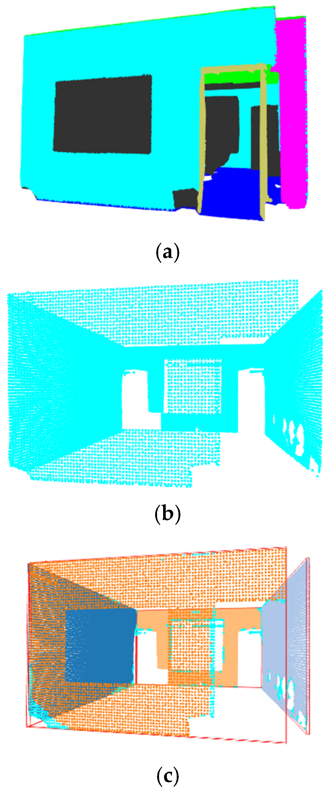
- Armeni, I.; Sener, O.; Zamir, A.R.; Jiang, H.; Brilakis, I.; Fischer, M.; Savarese, S. 3D Semantic Parsing of Large-Scale Indoor Spaces (a) Raw Point Cloud (b) Space Parsing and Alignment in Canonical 3D Space (c) Building Element Detection Enclosed Spaces. In Proceedings of the IEEE Conference on Computer Vision and Pattern Recognition, Las Vegas, NV, USA, 27–30 June 2016. [Google Scholar]
- S3DIS Benchmark (Semantic Segmentation)|Papers with Code. Available online: https://paperswithcode.com/sota/semantic-segmentation-on-s3dis (accessed on 20 January 2025).
- He, K.; Zhang, X.; Ren, S.; Sun, J. Deep Residual Learning for Image Recognition. In Proceedings of the 31st Annual Conference on Neural Information Processing Systems (NIPS 2017), Long Beach, CA, USA, 4–9 December 2017. [Google Scholar]
- Sandler, M.; Howard, A.; Zhu, M.; Zhmoginov, A.; Chen, L.-C. MobileNetV2: Inverted Residuals and Linear Bottlenecks. In Proceedings of the IEEE/CVF Conference on Computer Vision and Pattern Recognition, Salt Lake City, UT, USA, 18–23 June 2018. [Google Scholar]
- Chollet, F. Xception: Deep Learning with Depthwise Separable Convolutions. In Proceedings of the IEEE Conference on Computer Vision and Pattern Recognition, Honolulu, HI, USA, 21–26 July 2017. [Google Scholar]
- Vaswani, A.; Shazeer, N.; Parmar, N.; Uszkoreit, J.; Jones, L.; Gomez, A.N.; Kaiser, Ł.; Polosukhin, I. Attention Is All You Need. In Proceedings of the 31st Annual Conference on Neural Information Processing Systems (NIPS 2017), Long Beach, CA, USA, 4–9 December 2017; Available online: https://dl.acm.org/doi/10.5555/3295222.3295349 (accessed on 23 March 2025).
- Qian, G.; Al Kader Hammoud, H.A.; Li, G.; Thabet, A.; Ghanem, B. ASSANet: An Anisotropic Separable Set Abstraction for Efficient Point Cloud Representation Learning. Adv. Neural Inf. Process. Syst. 2021, 34, 28119–28130. [Google Scholar]
- Liu, Z.; Hu, H.; Cao, Y.; Zhang, Z.; Tong, X. A Closer Look at Local Aggregation Operators in Point Cloud Analysis; Lecture Notes in Computer Science (Including Subseries Lecture Notes in Artificial Intelligence and Lecture Notes in Bioinformatics); Springer: Cham, Switzerland, 2020; Volume 12368, pp. 326–342. [Google Scholar] [CrossRef]
- Bader, M. Space-Filling Curves; Springer: Berlin/Heidelberg, Germany, 2013; Volume 9. [Google Scholar] [CrossRef]
- Bassier, M.; Klein, R.; Van Genechten, B.; Vergauwen, M. IfcWall Reconstruction from Unstructured Point Clouds. ISPRS Ann. Photogramm. Remote Sens. Spat. Inf. Sci. 2018, 4, 33–39. [Google Scholar] [CrossRef]
- Yang, B.; Wang, J.; Clark, R.; Hu, Q.; Wang, S.; Markham, A.; Trigoni, N. Learning Object Bounding Boxes for 3D Instance Segmentation on Point Clouds. In Proceedings of the 33rd Conference on Neural Information Processing Systems (NeurIPS 2019), Vancouver, BC, Canada, 8–14 December 2019. [Google Scholar]
- IfcOpenShell—The Open Source IFC Toolkit and Geometry Engine. Available online: https://ifcopenshell.org/ (accessed on 20 January 2025).
- Open3D Primary (Unknown) Documentation. Available online: https://www.open3d.org/docs/latest/index.html (accessed on 18 March 2025).
- blender.org—Home of the Blender Project—Free and Open 3D Creation Software. Available online: https://www.blender.org/ (accessed on 13 February 2025).
- Bassier, M.; Vergauwen, M. Topology Reconstruction of BIM Wall Objects from Point Cloud Data. Remote Sens. 2020, 12, 1800. [Google Scholar] [CrossRef]
- Khoshelham, K.; Díaz-Vilariño, L. 3D Modelling of Interior Spaces: Learning the Language of Indoor Architecture. Int. Arch. Photogramm. Remote Sens. Spat. Inf. Sci. 2014, 40, 321–326. [Google Scholar] [CrossRef]


| PointNeXt | PointMetaBase | PTV1 | PTV3 | Swin3D | |
|---|---|---|---|---|---|
| Core Idea | Hierarchical feature learning | Meta Architecture | Point based Attention | Patch-based Attention | Shift Window Attention |
| Neighbour Search | FPS | KNN | KNN/Radius Search | Patch Partition | Sparse Voxelization Neighbour Lookup |
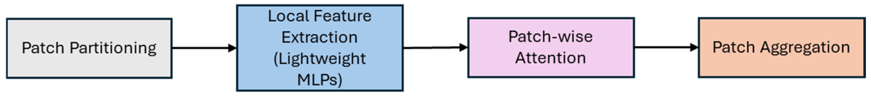
| Extract Features of Points | InvResMLPs | Lightweight MLPs | Vector Self Attention | Lightweight MLPs and Patch-wise Attention | Sparse Convolution |
| Spatial Encoding | Implicit | Explicit | Relative | Patch Interaction | cRSE |
| Neighbour Aggregation | Max Pooling/Stratified Sampling | Max Pooling | Attention Weights | Patch Aggregation | Shift Window Self-Attention |
| Algorithms | Swin3D | PTV3 | PTV1 | PointNeXt | PointMetaBase |
|---|---|---|---|---|---|
| mAcc (%) | 77.89 | 71.75 | 70.98 | 70.51 | 73.4 |
| oAcc (%) | 94.83 | 93.43 | 93.03 | 92.39 | 93.56 |
| mIoU (%) | 72.24 | 67.13 | 66.65 | 65.78 | 68.88 |
| Wall IoU (%) | 88.95 | 86.41 | 84.97 | 82.25 | 85.74 |
| Algorithms | Swin3D | PTV3 | PTV1 | PointNext | PointMetaBase |
|---|---|---|---|---|---|
| Mean Distance (m) | 0.073 | 0.077 | 0.085 | 0.077 | 0.078 |
| Max Distance (m) | 0.332 | 0.362 | 0.477 | 0.369 | 0.412 |
| Standard Deviation (m) | 0.068 | 0.075 | 0.098 | 0.070 | 0.078 |
Disclaimer/Publisher’s Note: The statements, opinions and data contained in all publications are solely those of the individual author(s) and contributor(s) and not of MDPI and/or the editor(s). MDPI and/or the editor(s) disclaim responsibility for any injury to people or property resulting from any ideas, methods, instructions or products referred to in the content. |
© 2025 by the authors. Licensee MDPI, Basel, Switzerland. This article is an open access article distributed under the terms and conditions of the Creative Commons Attribution (CC BY) license (https://creativecommons.org/licenses/by/4.0/).
Share and Cite
Patil, J.; Kalantari, M. Automatic Scan-to-BIM—The Impact of Semantic Segmentation Accuracy. Buildings 2025, 15, 1126. https://doi.org/10.3390/buildings15071126
Patil J, Kalantari M. Automatic Scan-to-BIM—The Impact of Semantic Segmentation Accuracy. Buildings. 2025; 15(7):1126. https://doi.org/10.3390/buildings15071126
Chicago/Turabian StylePatil, Jidnyasa, and Mohsen Kalantari. 2025. "Automatic Scan-to-BIM—The Impact of Semantic Segmentation Accuracy" Buildings 15, no. 7: 1126. https://doi.org/10.3390/buildings15071126
APA StylePatil, J., & Kalantari, M. (2025). Automatic Scan-to-BIM—The Impact of Semantic Segmentation Accuracy. Buildings, 15(7), 1126. https://doi.org/10.3390/buildings15071126