Deflection Predictions of Tapered Cellular Steel Beams Using Analytical Models and an Artificial Neural Network

Abstract

Cellular steel beams are primarily used to accommodate electrical and mechanical services within their structural depth, helping to reduce the floor-to-ceiling height in buildings. These beams are often tapered for various reasons, such as connecting members (e.g., beams) of different depths, adjusting stiffness in specific areas, or enhancing architectural design. This paper presents an algorithm developed using MATLAB R2019a and an artificial neural network (ANN) to predict the deflection of tapered cellular steel beams. The approach considers the web I-section variation parameter (α), along with shear and bending effects that contribute to additional deflections. It also accounts for the influence of the stiffness of the upper and lower T-sections at the centreline of the web opening. To validate the model, a total of 1415 finite element models were analysed. The deflections predicted by the analytical and ANN models were compared with finite element results, showing good agreement.

1. Introduction

Designers aim to optimize material usage for more economical and sustainable designs. In many cases, tapered steel elements offer a highly effective solution for both buildings and roof structures, especially when applied to long-span cantilevers, such as stadium stands, continuous beams, footbridges, or portal frame rafters.

Several studies have analysed the behaviour of prismatic perforated steel beams to provide engineers with approximate design formulas. However, tapered steel beams present a more complex analysis due to their geometry [1], (Figure 1). Integrating services and equipment within the structural floor depth has become common practice with the use of perforated beams, such as cellular and castellated beams [2]. These beams allow for passaging electric and hydraulic services through their openings, eliminating the need for running them beneath the sections [3,4]. Additionally, they are lighter and deeper than standard beams due to the material reduction from web openings, enabling longer spans without excessive deflection.

BS EN 1993-1-1 (2022) [5] and BS EN 1993-1-13 (2024) [6] do not offer specific guidelines for calculating the deflection of perforated beams, particularly for prismatic and non-prismatic steel beams with web openings. However, SCI-P355 [7] provides an approximate method for calculating additional deflection in beams with single or multiple openings. The Steel Design Guide 31 [8] provides a formula based on the radial stress method to estimate local deflection caused by web openings.

Researchers have increasingly used ANNs to predict the behaviour of structural components and systems. ANNs have proven effective in making accurate predictions across a range of structural applications.

Warren McCulloch and Walter Pitts were among the first to develop a neuron model in 1943, which was divided into two components. This foundational model remains integral to modern artificial neural networks (ANNs) [9,10].

ANNs have been applied to the analysis of perforated steel beams, which exhibit complex structural behaviour. Gholizadeh et al. [11] used an ANN with 140 finite element models to predict web-post capacity. Sharifi and Tohidi [12] developed an ANN-based formula to predict the buckling of steel girders with rectangular web openings. Tohidi and Sharifi [13,14] used an ANN to estimate the lateral–torsional buckling resistance of corroded steel beams. Other studies have focused on lateral–distortional buckling [15] and the bearing capacity of castellated beams [16]. Large datasets have been used to train ANN models; Abambres et al. [17] used 3645 finite element models and Ferreira et al. [18] used 768 models to predict lateral–torsional buckling resistance. Recent works by Shamass et al. [10] and others have continued to refine ANN models for web-post buckling resistance and ultimate load predictions of perforated steel beams [10,19].

Degtyarev and Tsavdaridis [20] developed ML models for calculating the buckling and ultimate loads of steel cellular beams. Unlike previous studies, which predominantly focused on constant-section perforated beams, this study integrates the novel parameter (α) into analytical and ANN models, enabling the accurate deflection prediction of tapered cellular beams with varying geometry. This approach uniquely bridges the gap between analytical simplicity and the computational precision of finite element methods.

This study aims to predict the total elastic deflection of tapered perforated steel I-beams with circular web openings using both ANN and analytical models. A dataset comprising 1438 finite element models was developed, simulating various loading conditions. The results from the proposed calculation methods and ANN models are validated against finite element models generated using the commercial software ABAQUS/CAE 2017 [21], focusing on elastic analysis.

This paper addresses a key research gap by proposing an analytical formulation for tapered steel beams with web openings, focusing on the additional deflection caused by multiple circular openings in the web of I-section beams under bending loads. The formulation introduces a new parameter to account for variations in the web I-section, which are often overlooked by traditional elastic models. It begins by calculating the additional deflection for a single circular opening, considering local shear and bending effects in the upper and lower Tee-sections. An algorithm is then applied to compute the total additional deflection for both the openings and solid tapered beams under various load conditions. The total deflection of the tapered cellular steel beam is determined by combining the deflection from the openings with that of the solid beam.

Figure 1. Application of tapered cellular steel beams in a real building [8].

Figure 1. Application of tapered cellular steel beams in a real building [8].

2. Prediction Models for Additional and Total Deflection

As previously mentioned, SCI-P355 [7] outlines an approximate approach for calculating the extra deflection caused by single and multiple openings in composite beams of constant sections. This method is based on an analytical technique for single web openings, which considers both additional bending deflection and additional shear deflection. Thus, the additional deflection for multiple regular openings is calculated according to Equation (1), in which $w_{add}$ is the total additional deflection for multiple regular openings, $w_b$ is the deflection of the solid beam, $n_0$ is the number of regular openings along the beam, $k_0$ is the coefficient equal to 1.0 for longitudinally stiffened and 1.5 for unstiffened openings, $h_0$ is the opening height, $h$ is the beam height, $l_0$ is the effective length of the opening, and L is the beam span.

$${\displaystyle \frac{w_{add}}{w_b}}=0.7\cdot n_0\cdot k_0\left({\displaystyle \frac{h_0}{h}}\right)\left({\displaystyle \frac{l_0}{L}}\right)$$

(1)

For the case of cellular beams, the effective length ($l_0$) of the opening is 0.45$h_0$. Thus,

$${\displaystyle \frac{w_{add}}{w_b}}=0.47\cdot n_0{\left({\displaystyle \frac{h_0}{h}}\right)}^2\left({\displaystyle \frac{h}{L}}\right)$$

(2)

These equations originate from the SCI P355 [7] guide, which provides a design method in accordance with Eurocode 3 [5] and Eurocode 4 [22]. These formulations were developed based on multiple research studies investigating the impact of web openings on beam stiffness and deflection.

However, the detailed derivation of these equations is not explicitly provided in the SCI P355 guide itself. Instead, they are empirical or semi-analytical formulations calibrated through numerical and experimental studies referenced within the guide. The works of several researchers, including Lawson [23,24,25], Ward [26], and Redwood, R.G [27], among others, provide in-depth insights into the effects of web openings on beam stiffness and deflection.

3. Proposed Model

The theoretical model proposed in this study focuses on tapered, thin-walled, bi-symmetric steel beams with circular, regularly spaced web openings of constant size. The beams are considered simply supported and subjected to three types of transverse loads: three-point bending, four-point bending, five-point loading, and cantilever beams with concentrated load ($P$) at the free end. The displacements of the steel beam sections are characterized by linear vertical ($w_x$) and angular (${\theta }_x$) displacements. The values of $w_x$ and ${\theta }_x$, which are in an arbitrary section of a prismatic beam with the constant section located at distance x from the origin, are given by Equations (3) and (4), respectively.

$$w_x=y=\iint {\displaystyle \frac{M_x}{EI}} {dx}^2 +{y\prime }_0 x+y_0$$

(3)

$${\theta }_x=y\prime =\int {\displaystyle \frac{M_x}{EI}} dx+{y\prime }_0$$

(4)

The maximum deflection of solid beams with a web-tapered section for the four load cases is given by Equations (5)–(8). These cases include three-point bending, four-point bending, and five-point bending for beams that are simply supported at both ends, as well as a cantilever beam.

$$w_x=y={\displaystyle \frac{P L^3}{48 E I_x}}$$

(5)

$$w_x=y={\displaystyle \frac{P a (3L^2-4a^2) }{24 E I_x}}$$

(6)

$$w_x=y={\displaystyle \frac{P L^3}{20.1 E I_x}}$$

(7)

$$w_x=y={\displaystyle \frac{P L^3}{3 E I_x}}$$

(8)

The diagram in Figure 2 illustrates the local bending and shear effects on the upper and lower tee-sections caused by the presence of circular web openings. The deflection is influenced by the tapered geometry of the beam, with the parameter ($\alpha$) representing the variation in web height (Equation (9)). Figure 2 highlights the Vierendeel mechanism, where stress concentrations occur around the openings, leading to additional deflections that must be accounted for in the structural analysis.

$$\alpha ={\displaystyle \frac{h_{min}}{h_{max}}}$$

(9)

In these equations, $h_{max}$ represents the distance between the outer edges of the two flanges at $x$ = $L$/2 (mid-span) for the simply supported beam, while $h_{min}$ is the distance between the outer edges of the two flanges at $x$ = 0 and $x$ = $L$ (the beam’s ends).

For the case of a cantilever beam, $h_{max}$ is located at the fixed end, whereas $h_{min}$ is located at the free end. Regarding the taper parameter ($\alpha$), it is evident that the case of a prismatic cross-section is covered by setting $\alpha$ = 1.

The deflection of tapered, thin-walled, bi-symmetric steel beams with circular web openings, subjected to bending and shear forces, is calculated by considering the additional deflection caused by the web openings, as illustrated in Figure 2. To accurately determine this additional deflection, the local bending deformation of the upper and lower tee-sections must also be accounted for.

The deflection due to bending in the upper and lower tee-sections is determined using Equations (9) and (10), where $i_f$, $i_{wx}$, and $i_x$ represent the moments of inertia of the flange, the tapered web, and the entire tee-section, respectively. The $\beta$ angle denotes the concentration of stresses along the edge of a circular web opening subjected to bending, with a local plasticised section (Vierendeel mechanism) forming in this area—specifically, the diagonal section connecting the top and bottom tee-sections. The length $l$ of the tee-section is modelled as a cantilever beam subjected to an external load ($V$) on its free end, calculated using Equations (10)–(14).

$$w_{ T,b}={\displaystyle \frac{V l^3}{3 E i_x}}$$

(10)

$$l=R \mathit{sin}\beta$$

(11)

$$i_f={\displaystyle \frac{b_f {t_f}^3}{12}}$$

(12)

$$i_{wx}={\displaystyle \frac{t_w{\left(\frac{h_{wx}-D}{2}\right)}^3}{12}}$$

(13)

$$i_x=i_f+A_f\cdot d_f^2+i_{wx}+A_{wx}\cdot d_{wx}^2$$

(14)

where $A_f$ denotes the area of the flange, $d_f$ denotes the distance between the centroid of the I-section and the centroid of the flange section, $A_{wx}$ denotes the area of the tapered web of the T-section, and $d_{wx}$ denotes distance between the centroid of the I-section and the centroid of the web-tapered T-section.

Lawson et al. [25] and Tsavdaridis et al. [28] estimated that $\beta$, the angle of stress concentration, ranges between 25° and 40° for perforated steel beams with circular web openings, depending on the shear-to-moment ratio at the web opening’s centreline. This study acknowledges that the Vierendeel mechanism is not fully developed for circular web openings, especially those with smaller diameters. The Vierendeel effect is more significant in rectangular openings than circular ones. In this work, a 45° angle is adopted, treating the circular openings as equivalent to a rectangular shape, in line with UK standards.

The deflection under the shear effect of the upper and lower tee-sections is given by Equations (15)–(18):

$$w_{T,s}={\displaystyle \frac{V l}{G {\omega }_x}}$$

(15)

$$G={\displaystyle \frac{E}{2\cdot (1+\upsilon )}}$$

(16)

$${\omega }_x={\displaystyle \frac{\left(h_{wx}-2R\right)}{2}}\cdot t_w$$

(17)

$$h_{wx}=H_{wx}-2 t_f$$

(18)

It is assumed that the two local additional deflections are equivalent for the upper and lower tee-sections of the beam at the opening, according to Equation (19).

$$w_T=w_{T,top}=w_{T,bottom}=w_{T,b}+w_{T,s}$$

(19)

The total additional deflection ($w_{add}$) at a single opening of the beam, which considers the effect of bending and shear deformation, is given by Equation (20):

$$w_{add}=2\left(w_{T,b}+w_{T,s}\right)$$

(20)

The expression for the additional deflection of a beam with web openings is valid only for a single opening. Unlike the approach in SCI-P355 [7], this study examines beams with periodic circular web openings, accounting for local geometric variations due to the tapered factor. The total additional deflection of a cellular beam is determined by summing the individual deflections of each web opening. To achieve this, a MATLAB R2019a algorithm [29] was developed, using a loop parameterized by the index $i$, which calculates the deflection for all $n$ openings at the midspan. The loop runs from 1 to $m$, where $m$ = 2 $n$, and the positions $x$ of the openings along the beam’s length are determined at even i-values, calculated using Equation (21), as shown in Figure 3.

$$x_{even}={\displaystyle \frac{i}{2}}W+\left(i-1\right){\displaystyle \frac{D}{2}}$$

(21)

Also, for each even pitch of $i$, the local additional deflections due to shear ($w_{Ts,i}$) and bending ($w_{Tb,i}$) are calculated; thus, the local additional deflection for opening $i$ is calculated according to Equation (22):

$$w_{add, i}=2\left(w_{Tb,i}+w_{Ts,i}\right)$$

(22)

Consequently, the total additional deflection of all openings of the cellular beams can be predicted by Equation (23):

$$w_{add}=\sum _{i=0}^m{w}_{add,i}$$

(23)

Currently, no analytical expression exists for calculating the deflection of unperforated (solid web) tapered beams. Instead, deflection ($w_0$) is computed using a numerical finite element model based on the Euler–Bernoulli approach, developed for four different loading cases and various tapered web section parameters. The total deflection ($w$) of the tapered cellular steel beam is then determined using Equation (24).

$$w=w_0+w_{add}$$

(24)

4. Finite Element Method

The deflection values obtained from the proposed method in Section 3 are compared with the results from finite element simulations using ABAQUS/CAE 2017 [21].

The numerical model was validated against the proposed analytical method and SCI-P355 for prismatic beams. The results are presented and discussed in Section 8. Its application to tapered cellular beams showed strong agreement between the numerical and analytical results, confirming the method’s reliability.

The numerical model was developed for elastic analysis using Static General, where the linear problem is solved via the Newton–Raphson method. The initial load increment was set to 10% of the total external load applied to the structure, with the analysis concluding once 100% of the load was reached. The elastic properties of the steel used in the study included a modulus of elasticity of 210 GPa and a Poisson’s ratio of 0.3.

Figure 4 illustrates the boundary conditions for three-point bending, where the beams are considered simply supported. One end has displacements fully restrained in all three directions ($U_x$ = $U_y$ = $U_z$ = 0), while the other end has displacements restrained in two directions ($U_y$ = $U_z$ = 0) [30,31].

The I-sections were discretized using eight-node quadrilateral shell elements (S8R), each with six degrees of freedom per node (three translations and three rotations). This element was employed for its ability to provide accurate results with reduced computational effort [30,32]. A free mesh rule was applied, and a sensitivity analysis was conducted by varying the mesh element size.

Table 1. Mesh sensitivity analysis.

α	L (m)	P (kN)	Section	n	Deflection (mm)				Δ (%)			CPU Run-Time (s)
					Mesh Size			Proposed Method				Mesh Size
					10	20	40		10.00	20.00	40.00	10	20	40
0.4	6	100	IPE600	24	4.43	4.42	4.39	4.183	5.58	5.36	4.72	29.4	5.7	1.3
	8	100	IPE600	32	9.85	9.83	9.79	9.094	7.68	7.49	7.11	48.2	10.8	2.1
	12	100	IPE600	48	31.61	31.59	31.52	28.417	10.10	10.04	9.84	67.2	12.2	2.5
0.6	6	100	IPE600	14	4.05	4.04	4.02	3.905	3.58	3.34	2.86	38.7	7.7	1.3
	8	100	IPE600	20	8.69	8.69	8.66	8.471	2.52	2.52	2.18	40.3	10	1.9
	12	100	IPE600	30	27.2	27.19	27.14	26.133	3.92	3.89	3.71	66	15.2	3.7
0.8	6	100	IPE600	10	3.93	3.93	3.91	3.878	1.32	1.32	0.82	33.6	9.6	2.4
	8	100	IPE600	14	8.2	8.2	8.18	8.053	1.79	1.79	1.55	50.3	12.7	2
	12	100	IPE600	20	24.62	24.61	24.58	24.130	1.99	1.95	1.83	66	15.5	3.2

shows the deflections and CPU run-time for three different mesh sizes applied to IPE600 section beams with three different tapered section parameters ($\alpha$) under three-point bending with simply supported conditions. The parameter $\alpha$ represents the tapered factor of the beam’s cross-section and is calculated as the ratio of the minimum to maximum web height. In ABAQUS/CAE 2017, this parameter is incorporated by defining variable cross-section properties along the beam’s length, aligning with the input geometry and load distribution.

The results indicate that changes in mesh size have a minimal impact on deflection predictions. Based on the sensitivity analysis, a mesh size of 20 mm was selected for the parametric study. The processing time for each mesh shown in Table 1 varied with mesh size. For the smallest mesh, the time was 67.2 s, while for the largest, it was around 3.7 s. However, processing time did not significantly affect the number of analyses performed, as the mesh size was selected based on accuracy results rather than processing speed.

Regarding the parametric study, the loads were applied to the upper flanges of the cellular beams, considering three- and four-point bending load cases, as shown in Figure 5. The length of the beams varies between 4.702 m and 12.0 m to represent typical spans. The deflections are evaluated for the tapered section parameters ($\alpha$ = 0.4, 0.6, and 0.8). The analysis uses typical steel sections such as IPE600, IPE550, IPE500, and IPE450. The diameter of the circular web openings of the cellular beams is 75% of the beam’s total height, excluding the flange thickness. The number of openings ranges from 10 to 18, depending on the beam’s span, with uniform spacing along the beam length. Notably, no openings are placed at the mid-span. Deflections are measured at the mid-span on the bottom flange of the beams.

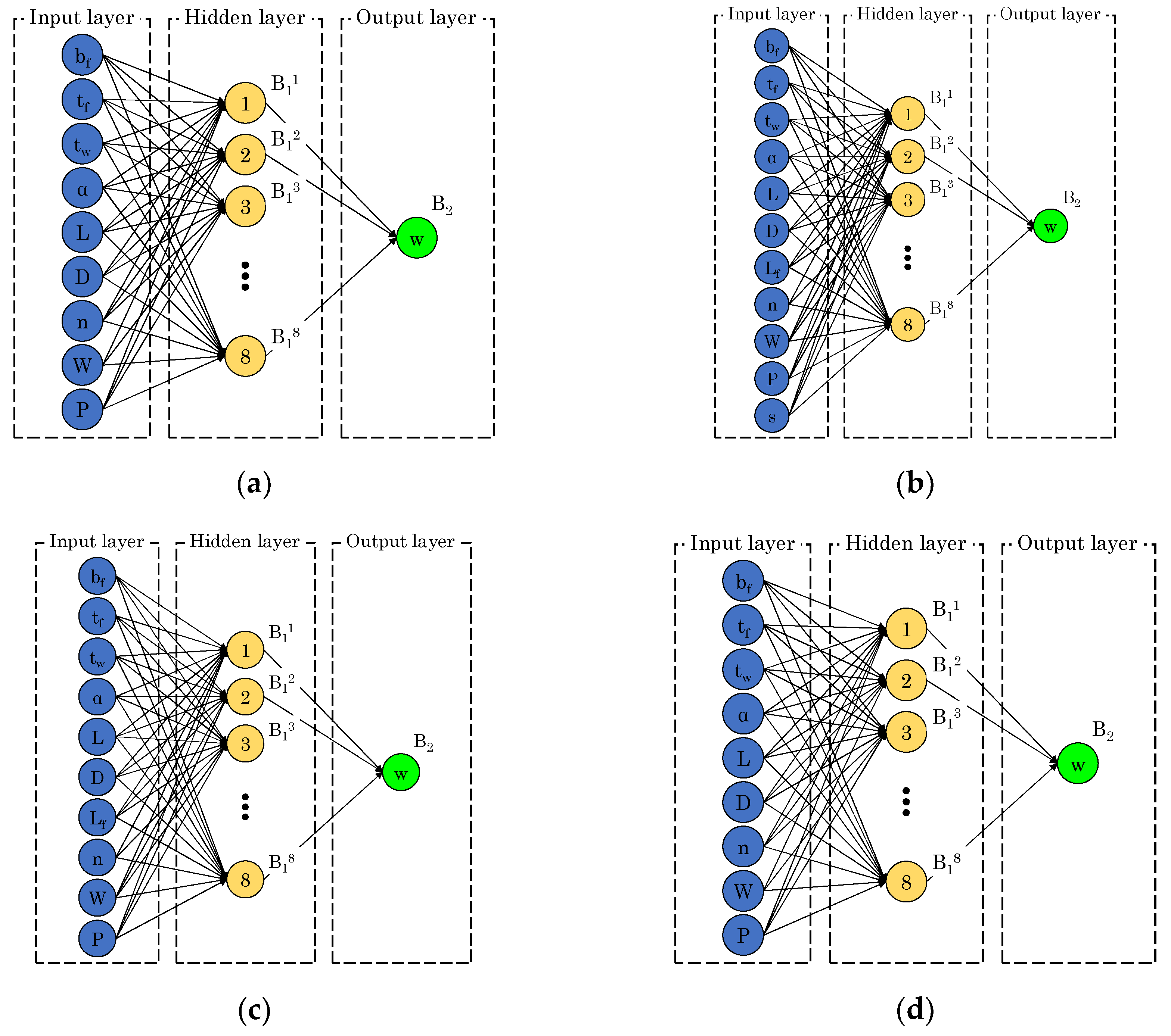
5. Artificial Neural Network

A dataset of 1415 finite element models was used to predict the deflections of the tapered cellular steel beams using an ANN. The ANN model used in this study employs a feedforward architecture with Levenberg–Marquardt backpropagation for training. It maps input variables to predict deflections, optimizing accuracy through iterative weight adjustments. The ANN-based formulas infer deflections by normalizing input variables and applying trained weights and bias terms to compute outputs. Each formula corresponds to specific loading conditions, ensuring tailored predictions across various scenarios. The input parameters for developing the ANN include flange width ($b_f$), flange thickness ($t_f$), tapered section factor ($\alpha$), beam span ($L$), opening diameter ($D$), load distance ($L_f$), number of openings ($n$), spacing between openings ($W$), load ($P$), and shear span ($s$). The study models the ANN with four, six, and eight neurons in the hidden layer. While the proposed analytical model offers a manual computation approach, the inclusion of the ANN is essential for scenarios requiring rapid predictions across a wide range of parameters. The ANN can achieve an approximate 5% improvement in accuracy, which is critical for engineering applications where precision directly influences structural integrity and cost-effectiveness. Figure 6 illustrates the ANN structure, showing the input parameters for each loading case, the number of hidden layer neurons, and a single output parameter.

The normalization of input variables is applied following the method by Moradi et al. [33], as described in Equation (25) [34]. In this equation, $X^{act}$ represents the actual value and $X^{norm}$ is the normalized value, while $X_{min}$ and $X_{max}$ are the minimum and maximum values of the input/output parameters. $Y_{min}$ and $Y_{max}$ are the minimum (default is −1) and maximum (default is +1) values for each row of $X$. The output parameters are then denormalized, with $X^{act}$ derived from the equation, and $X^{norm}$ being the predicted value from the ANN model.

Table 2. Parameters used to normalize input and target values.

Input/Target Parameter	Xmin	Xmax	Ymin	Ymax
bf (mm)	190	220	−1	1
tf (mm)	14.6	19	−1	1
tw (mm)	5	17.2	−1	1
α	0.4	1	−1	1
L (mm)	4702	12,000	−1	1
D (mm)	130	353.6	−1	1
n	10	58	−1	1
Lf (mm)	1175.5	6000	−1	1
W (mm)	66	450	−1	1
a P (kN)	1.67	180	−1	1
a s (mm)	1175.5	6000	−1	1

^a Varies according to loading conditions.

lists all parameters used.

$$X^{norm}={\displaystyle \frac{\left(Y_{max}-Y_{min}\right)\left(X^{act}-X_{min}\right)}{\left(X_{max}-X_{min}\right)}}+Y_{min}$$

(25)

A multilayer feedforward neural network is designed and trained using the Levenberg–Marquardt backpropagation algorithm, which is memory-intensive but efficient in execution time. The ANN model employs a dataset of 1415 finite element models divided into two subsets: 70% for training and 30% for testing. This division ensures an adequate test set for validating the model with new data while minimizing the risk of overfitting during training.

The hyperbolic tangent transfer function (tansig) was employed, as it is well suited for capturing non-linear relationships in data [33] and is readily available in MATLAB R2019a.

The reliability of the developed model is assessed by comparing the target and predicted values using several metrics. The correlation coefficient ($R$), Root Mean Square Error (RMSE), and Mean Absolute Error (MAE) are calculated according to Equations (26)–(28), in which $t_i$ and $O_i$ are the actual and predicted deflections, $N$ is the total number of data points in each set of data, and $\overline{O}$ and $\overline{t}$ are the average of the predicted and actual deflections.

$$R={\displaystyle \frac{\sum _{i=1}^N\left(O_i-{\overline{O}}_i\right)\left(t_i-{\overline{t}}_i\right)}{\sqrt{\sum _{i=1}^N{\left(O_i-{\overline{O}}_i\right)}^2 \sum _{i=1}^N{\left(t_i-{\overline{t}}_i\right)}^2}}}$$

(26)

$$RMSE=\sqrt{{\displaystyle \frac{\sum _{i=1}^N{\left(O_i-t_i\right)}^2}{N}}}$$

(27)

$$MAE={\displaystyle \frac{1}{N}}\sum _{i=1}^N\left|O_i-t_i\right|$$

(28)

The analysis of how input parameters affect the deflection of tapered cellular steel beams is conducted using the connection weight approach (proposed by Olden and Jackson [35]) according to Equation (29), in which $X$ is the input parameter, $Y$ is the weighted connection between the input parameter and the hidden layer, and Hidden is the weighted connection between the hidden layer and the output parameter. This method has been referenced in other studies as well [10,18,36].

$${Input}_X=\sum _{Y=A}^E{Hidden}_{XY}$$

(29)

The significance of each input variable in the ANN is assessed using Garson’s algorithm [37], which has been referenced in various studies [38,39,40]. Equation (30) quantifies the importance of the $j^{th}$ input parameter on the output, in which $N_i$ and $N_h$ are the numbers of neurons in the input and hidden layers, respectively, $w$ is connection weight, $k$, $m$, and $n$ refer to the input, hidden, and output neurons, respectively, and $i$, $h$, and $o$ refer to the input, hidden, and output layers, respectively.

$$I_j={\displaystyle \frac{\sum _{m=1}^{m=Nh}\left(\frac{w_{jm}^{ih}}{\sum _{k=1}^{Ni}{w}_{km}^{ih}}{w}_{mn}^{ho}\right)}{\sum _{k=1}^{k=Ni}\left[\sum _{m=1}^{m=Nh}\left(\frac{w_{km}^{ih}}{\sum _{k=1}^{Ni}{w}_{km}^{ih}}{w}_{mn}^{ho}\right)\right]}}$$

(30)

6. Results and Discussion

The results are discussed in terms of how additional and total deflections are influenced by the number of openings and the development of the ANN.

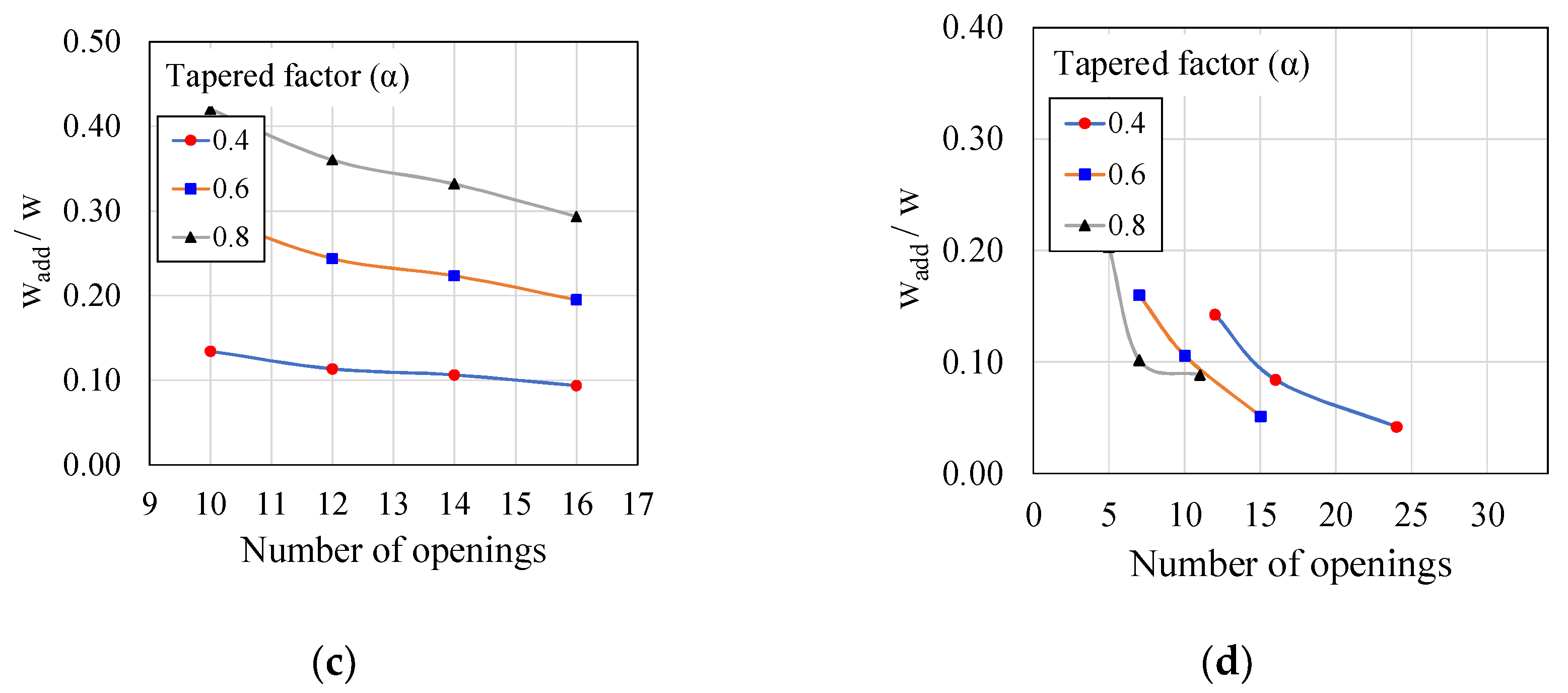
6.1. Additional Deflection

Figure 7 illustrates the relationship between the ratio of additional deflection ($w_t$) to total deflection ($w$) as a function of the number of openings under various loading conditions: three-point bending (Figure 7a), four-point bending (Figure 7b), five-point bending (Figure 7c), and cantilever loading (Figure 7d). As the number of openings and the span increase, the influence of additional deflection on the total deflection of cellular beams diminishes. In the cellular beams studied in this article, the openings are uniformly spaced and have a constant diameter along the span. Consequently, the stiffness of the Tee-section increases toward the mid-span of the beam. Our analytical formulation for calculating the additional deflection evaluates it at each opening, considering the exact force applied at that location. Due to the increasing stiffness of the Tee-section toward the centre of the beam, the additional deflection progressively decreases at each opening.

Therefore, fewer openings lead to a more significant impact on total deflection, consistent with the behaviour observed in prismatic perforated beams, as noted by Tsavdaridis and D’Mello [41]. Additionally, the opening diameter and the width of the web-post are based on the height of the web I-section, as shown in Figure 3. Furthermore, when the tapered section factor decreases, the effect of web openings on total elastic deflection also decreases, as the deflection at the tee-section becomes less critical and the Vierendeel effect diminishes.

The influence of loading conditions on total deflection shows similar behaviour across different scenarios. Under the same applied load, the additional deflection in three-point bending is significantly greater than in four-point bending, with increases ranging from 44% to 111%. In three-point bending, global shear remains constant, while the bending moment varies across the span, leading to a moment–shear interaction. Conversely, in four-point bending, the central span experiences null global shear and a constant bending moment, resulting in no shear–moment interaction in that area. Consequently, the Vierendeel effect is more pronounced in the three-point bending case.

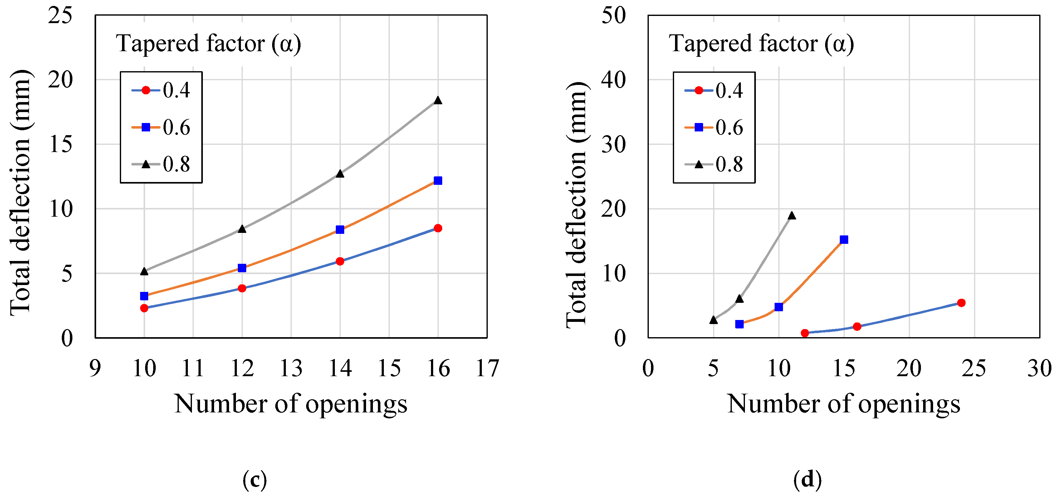
6.2. Total Deflection

Several examples illustrate the relationship between total deflection and the number of openings under different loading conditions (Figure 8), including three-point bending (Figure 8a), four-point bending (Figure 8b), five-point bending (Figure 8c), and cantilever loading (Figure 8d). Notably, an increase in the number of openings leads to a higher total deflection. Conversely, a reduction in the section factor results in smaller total deflections. This indicates that a smaller opening diameter increases the amount of steel used in the member, thereby enhancing the moment of inertia at the strong axis.

6.3. Prediction-Based ANN

Table 3. Accuracy of the ANN models with different numbers of neurons.

	3 Points			4 Points
Number of neurons	4	6	8	4	6	8
Max error	36.41	26.28	68.52	29.91	33.26	12.21
Min error	−24.48	−24.86	−28.64	−56.84	−22.13	−68.88
R2	0.99970	0.99993	0.99980	0.99940	0.9999	0.9999
RMSE	0.632	0.262	0.274	0.309	0.108	0.0997
	5 points			Cantilever
Number of neurons	4	6	8	4	6	8
Max error	45.57	13.44	70.52	4.56	3.18	1.49
Min error	−26.40	−11.40	−60.09	−1.96	−1.46	−0.62
R2	0.9995	0.9999	0.9995	0.99976	0.99993	0.99999
RMSE	0.288	0.121	0.627	0.0188	0.023	0.008

displays the comparison of the ANN results with the finite element models, using four, six, and eight neurons based on $R^2$ and RMSE metrics. The results show a distinct correlation between the model’s accuracy and the number of neurons in the hidden layer. Specifically, as the number of neurons increases, the model’s accuracy improves. However, an excessive number of neurons may lead to a more complex model, potentially resulting in overfitting.

The possibility of using fewer neurons (one or two) was initially explored, but performance metrics revealed that while this could simplify the model, it would likely compromise accuracy and reliability. Consequently, a compromise was made by selecting four, six, and eight neurons for optimal performance. The training process was repeated multiple times to address the inherent variability in machine learning, and the reported RMSE values reflect the average across these runs. For example, the higher RMSE for the five-point bending scenario with eight neurons compared to six is attributed to this variability.

The final RMSE values for the six-neuron model were as follows: $R^2$ = 0.99993 and RMSE = 0.262 for three-point beams; $R^2$ = 0.9999 and RMSE = 0.108 for four-point beams; $R^2$ = 0.9999 and RMSE = 0.121 for five-point beams; and $R^2$ = 0.99993 and RMSE = 0.023 for cantilever beams. These results indicate that the six-neuron model achieves a very high level of accuracy, making it effective for predicting outcomes. The high $R^2$ values (>0.99) indicate strong model performance. Overfitting risks were mitigated by dividing the dataset into 70% training and 30% testing, ensuring the model generalizes well to unseen data.

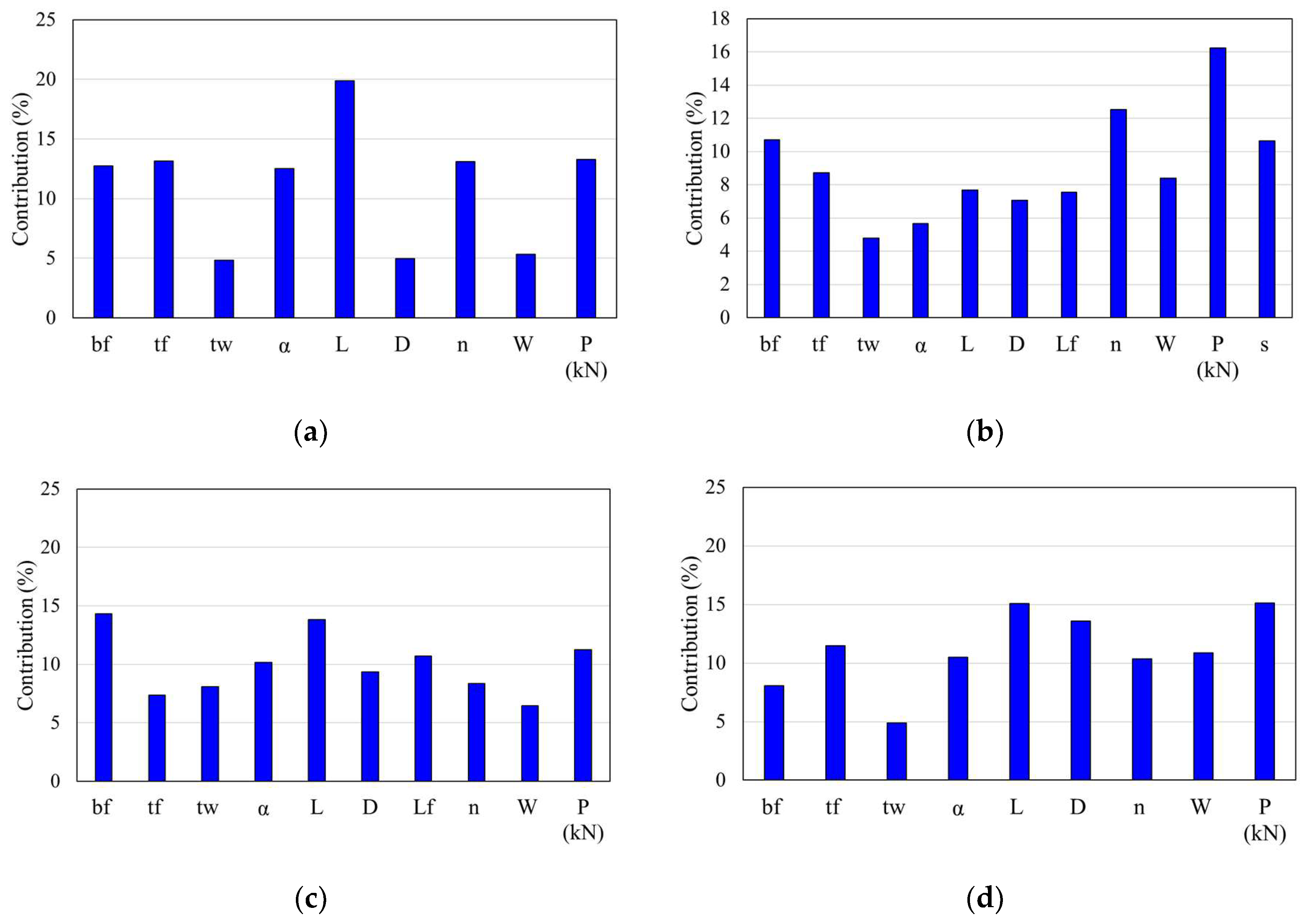
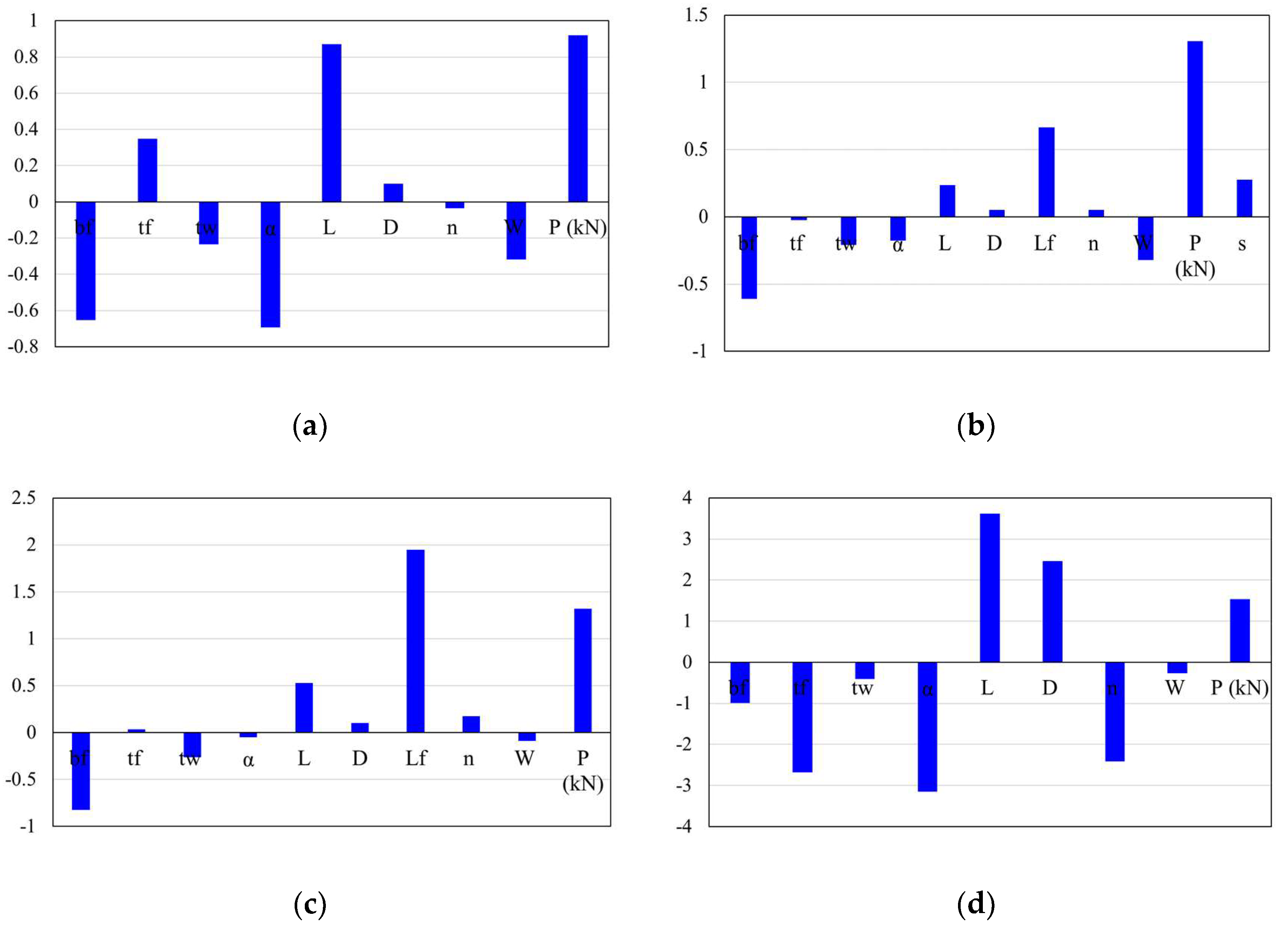
6.3.1. Variable Contribution

Figure 9 shows the importance of input parameters for deflection calculations. The most significant parameter is identified by the highest contribution value, as determined using Garson’s algorithm. For three-point bending beams (Figure 9a), the load ($P$), flange width ($b_f$), and span ($L$) are the key contributors, with percentage contributions of 19.9%, 13.3%, and 13.17%, respectively. In contrast, the distance between openings, web thickness, and section height have lesser impacts, contributing only 5.3%, 4.9%, and 5.0%, respectively.

For four-point bending beams (Figure 9b), the importance ranking is as follows: $P$ (16.2%), number of openings ($n$) (12.5%), $b_f$ (10.7%), and span ($s$) (10.6%), among others. In five-point bending beams (Figure 9c), the most influential parameters are $b_f$ and $L$, while the distance between openings ($W$) has the least significant effect at 6.5%. For cantilever beams (Figure 9d), the most impactful parameters are $P$, $L$, and diameter ($D$), while web thickness ($t_w$) has the least effect.

The influence of input parameters varies by beam type. For example, n contributes 13.1%, 12.5%, 8.4%, and 10.4% to the deflections in three-point, four-point, five-point, and cantilever beams, respectively. The contribution of flange width ($b_f$) ranges from 10.7% to 14.3% for simply supported beams, compared to 8.1% for cantilever beams. Overall, both $L$ and $P$ significantly affect deflections across all beam types.

6.3.2. Impact of Input Parameters on Deflection

Figure 10 displays the results from the connection weight approach, demonstrating the effect of each input parameter on the output for all models studied. The findings reveal consistent patterns in identifying which parameters significantly influence deflections and whether their effects are positive or negative.

For all beam types, increasing the span ($L$), load ($P$), and opening diameter ($D$) leads to higher deflections. This is explained by Equations (10) and (15), which incorporate the local shear force ($V$) derived from the overall load and recognize that a larger diameter increases the effective length, enhancing local deflections. Consequently, the Vierendeel effect accounts for both parameters. Additionally, as the number of web openings increases with the span, the total additional deflection also rises due to a higher number of local additional deflections, as indicated in Equation (23).

Conversely, parameters such as flange width ($b_f$), distance between openings ($W$), and tapered factor ($\alpha$) negatively affect deflections. The main equations calculating additional deflection do not include the width of the web-post ($W$). Both $b_f$ and $\alpha$ influence the stiffness of the tee-section in the perforated profiles, as seen in the denominators of Equations (10) and (15). However, $b_f$ has a minor effect on additional deflection since it remains constant along the beam, resulting in minimal variation in stiffness. Regarding $\alpha$, while openings are uniformly spaced, the stiffness of the tee-section becomes more significant toward the beam’s centre, where local additional deflection influences are counterproductive.

6.3.3. ANN-Based Formula

For each loading condition examined, a separate ANN-based formula was created to predict the deflection of tapered cellular steel beams, as outlined in Equations (31)–(34) for the three-point bending, four-point bending, five-point bending, and cantilever scenarios.

The ANN model automates the application of these design equations, improving prediction accuracy and reducing computational time [36]. The process involves the following:

• Input Data Collection: Geometric and loading parameters such as flange width, web thickness, taper factor, beam span, and number of openings.
• ANN Model Execution: Normalised inputs are fed into the trained ANN model for deflection predictions.

This approach bridges the gap between theoretical models and practical design, enhancing the efficiency and accuracy of structural analysis.

$$\begin{array}{l}{\left({\mathrm{w}}_{\mathrm{A}\mathrm{N}\mathrm{N}}\right)}_{\mathrm{n}}={\mathrm{B}}_2+{\sum }_{\mathrm{i}=1}^{\mathrm{n}=6}{\mathrm{w}}_2\left(\mathrm{i}\right)\left({\displaystyle \frac{2}{1+{\mathrm{e}}^{-2{\mathrm{H}}_{\mathrm{i}}}}}-1\right)\\ {\mathrm{H}}_{\mathrm{i}}={\mathrm{B}}_1\left(\mathrm{i}\right)+{\mathrm{w}}_1\left(\mathrm{i},1\right){\left({\mathrm{b}}_{\mathrm{f}}\right)}_{\mathrm{n}}+{\mathrm{w}}_1\left(\mathrm{i},2\right){\left({\mathrm{t}}_{\mathrm{f}}\right)}_{\mathrm{n}}+{\mathrm{w}}_1\left(\mathrm{i},3\right){\left({\mathrm{t}}_{\mathrm{w}}\right)}_{\mathrm{n}}+{\mathrm{w}}_1\left(\mathrm{i},4\right){\left(\mathrm{\alpha }\right)}_{\mathrm{n}}+{\mathrm{w}}_1\left(\mathrm{i},5\right){\left(\mathrm{L}\right)}_{\mathrm{n}}\\ \hspace{1em}\hspace{1em}\hspace{1em}\hspace{1em}\hspace{1em}\hspace{1em}\hspace{1em}+{\mathrm{w}}_1\left(\mathrm{i},6\right){\left(\mathrm{D}\right)}_{\mathrm{n}}+{\mathrm{w}}_1\left(\mathrm{i},7\right){\left(\mathrm{n}\right)}_{\mathrm{n}}+{\mathrm{w}}_1\left(\mathrm{i},8\right){\left(\mathrm{W}\right)}_{\mathrm{n}}+{\mathrm{w}}_1\left(\mathrm{i},9\right){\left(\mathrm{P}\right)}_{\mathrm{n}}\end{array}$$

(31)

$$\begin{array}{l}{\left({\mathrm{w}}_{\mathrm{A}\mathrm{N}\mathrm{N}}\right)}_{\mathrm{n}}={\mathrm{B}}_2+{\sum }_{\mathrm{i}=1}^{\mathrm{n}=6}{\mathrm{w}}_2\left(\mathrm{i}\right)\left({\displaystyle \frac{2}{1+{\mathrm{e}}^{-2{\mathrm{H}}_{\mathrm{i}}}}}-1\right)\\ {\mathrm{H}}_{\mathrm{i}}={\mathrm{B}}_1\left(\mathrm{i}\right)+{\mathrm{w}}_1\left(\mathrm{i},1\right){\left({\mathrm{b}}_{\mathrm{f}}\right)}_{\mathrm{n}}+{\mathrm{w}}_1\left(\mathrm{i},2\right){\left({\mathrm{t}}_{\mathrm{f}}\right)}_{\mathrm{n}}+{\mathrm{w}}_1\left(\mathrm{i},3\right){\left({\mathrm{t}}_{\mathrm{w}}\right)}_{\mathrm{n}}+{\mathrm{w}}_1\left(\mathrm{i},4\right){\left(\mathrm{\alpha }\right)}_{\mathrm{n}}+{\mathrm{w}}_1\left(\mathrm{i},5\right){\left(\mathrm{L}\right)}_{\mathrm{n}}\\ \hspace{1em}\hspace{1em}\hspace{1em}\hspace{1em}\hspace{1em}\hspace{1em}\hspace{1em}+{\mathrm{w}}_1\left(\mathrm{i},6\right){\left(\mathrm{D}\right)}_{\mathrm{n}}+{\mathrm{w}}_1\left(\mathrm{i},7\right){\left({\mathrm{L}}_{\mathrm{f}}\right)}_{\mathrm{n}}+{\mathrm{w}}_1\left(\mathrm{i},8\right){\left(\mathrm{n}\right)}_{\mathrm{n}}+{\mathrm{w}}_1\left(\mathrm{i},9\right){\left(\mathrm{W}\right)}_{\mathrm{n}}\\ \hspace{1em}\hspace{1em}\hspace{1em}\hspace{1em}\hspace{1em}\hspace{1em}\hspace{1em}+{\mathrm{w}}_1\left(\mathrm{i},10\right){\left(\mathrm{P}\right)}_{\mathrm{n}}+{\mathrm{w}}_1\left(\mathrm{i},11\right){\left(\mathrm{s}\right)}_{\mathrm{n}}\end{array}$$

(32)

$$\begin{array}{l}{\left({\mathrm{w}}_{\mathrm{A}\mathrm{N}\mathrm{N}}\right)}_{\mathrm{n}}={\mathrm{B}}_2+{\sum }_{\mathrm{i}=1}^{\mathrm{n}=6}{\mathrm{w}}_2\left(\mathrm{i}\right)\left({\displaystyle \frac{2}{1+{\mathrm{e}}^{-2{\mathrm{H}}_{\mathrm{i}}}}}-1\right)\\ {\mathrm{H}}_{\mathrm{i}}={\mathrm{B}}_1\left(\mathrm{i}\right)+{\mathrm{w}}_1\left(\mathrm{i},1\right){\left({\mathrm{b}}_{\mathrm{f}}\right)}_{\mathrm{n}}+{\mathrm{w}}_1\left(\mathrm{i},2\right){\left({\mathrm{t}}_{\mathrm{f}}\right)}_{\mathrm{n}}+{\mathrm{w}}_1\left(\mathrm{i},3\right){\left({\mathrm{t}}_{\mathrm{w}}\right)}_{\mathrm{n}}+{\mathrm{w}}_1\left(\mathrm{i},4\right){\left(\mathrm{\alpha }\right)}_{\mathrm{n}}+{\mathrm{w}}_1\left(\mathrm{i},5\right){\left(\mathrm{L}\right)}_{\mathrm{n}}\\ \hspace{1em}\hspace{1em}\hspace{1em}\hspace{1em}\hspace{1em}\hspace{1em}\hspace{1em}+{\mathrm{w}}_1\left(\mathrm{i},6\right){\left(\mathrm{D}\right)}_{\mathrm{n}}+{\mathrm{w}}_1\left(\mathrm{i},7\right){\left({\mathrm{L}}_{\mathrm{f}}\right)}_{\mathrm{n}}+{\mathrm{w}}_1\left(\mathrm{i},8\right){\left(\mathrm{n}\right)}_{\mathrm{n}}+{\mathrm{w}}_1\left(\mathrm{i},9\right){\left(\mathrm{W}\right)}_{\mathrm{n}}\\ \hspace{1em}\hspace{1em}\hspace{1em}\hspace{1em}\hspace{1em}\hspace{1em}\hspace{1em}+{\mathrm{w}}_1\left(\mathrm{i},10\right){\left(\mathrm{P}\right)}_{\mathrm{n}}\end{array}$$

(33)

$$\begin{array}{l}{\left({\mathrm{w}}_{\mathrm{A}\mathrm{N}\mathrm{N}}\right)}_{\mathrm{n}}={\mathrm{B}}_2+{\sum }_{\mathrm{i}=1}^{\mathrm{n}=6}{\mathrm{w}}_2\left(\mathrm{i}\right)\left({\displaystyle \frac{2}{1+{\mathrm{e}}^{-2{\mathrm{H}}_{\mathrm{i}}}}}-1\right)\\ {\mathrm{H}}_{\mathrm{i}}={\mathrm{B}}_1\left(\mathrm{i}\right)+{\mathrm{w}}_1\left(\mathrm{i},1\right){\left({\mathrm{b}}_{\mathrm{f}}\right)}_{\mathrm{n}}+{\mathrm{w}}_1\left(\mathrm{i},2\right){\left({\mathrm{t}}_{\mathrm{f}}\right)}_{\mathrm{n}}+{\mathrm{w}}_1\left(\mathrm{i},3\right){\left({\mathrm{t}}_{\mathrm{w}}\right)}_{\mathrm{n}}+{\mathrm{w}}_1\left(\mathrm{i},4\right){\left(\mathrm{\alpha }\right)}_{\mathrm{n}}+{\mathrm{w}}_1\left(\mathrm{i},5\right){\left(\mathrm{L}\right)}_{\mathrm{n}}\\ \hspace{1em}\hspace{1em}\hspace{1em}\hspace{1em}\hspace{1em}\hspace{1em}\hspace{1em}+{\mathrm{w}}_1\left(\mathrm{i},6\right){\left(\mathrm{D}\right)}_{\mathrm{n}}+{\mathrm{w}}_1\left(\mathrm{i},7\right){\left(\mathrm{n}\right)}_{\mathrm{n}}+{\mathrm{w}}_1\left(\mathrm{i},8\right){\left(\mathrm{W}\right)}_{\mathrm{n}}+{\mathrm{w}}_1\left(\mathrm{i},9\right){\left(\mathrm{P}\right)}_{\mathrm{n}}\end{array}$$

(34)

In these expressions, the parameters ${\left({\mathrm{b}}_{\mathrm{f}}\right)}_{\mathrm{n}}$, ${\left({\mathrm{t}}_{\mathrm{f}}\right)}_{\mathrm{n}}$, ${\left({\mathrm{t}}_{\mathrm{w}}\right)}_{\mathrm{n}}$, ${\left(\mathrm{\alpha }\right)}_{\mathrm{n}}$, ${\left(\mathrm{L}\right)}_{\mathrm{n}}$, ${\left(\mathrm{D}\right)}_{\mathrm{n}}$, ${\left({\mathrm{L}}_{\mathrm{f}}\right)}_{\mathrm{n}}$, ${\left(\mathrm{n}\right)}_{\mathrm{n}}$, ${\left(\mathrm{W}\right)}_{\mathrm{n}}$, ${\left(\mathrm{P}\right)}_{\mathrm{n}}$, and ${\left(\mathrm{s}\right)}_{\mathrm{n}}$ represent the normalised values of the inputs ${\mathrm{b}}_{\mathrm{f}}$, ${\mathrm{t}}_{\mathrm{f}}$, ${\mathrm{t}}_{\mathrm{w}}$, $\alpha$, $L$, $D$, $L_f$, $n$, $W$, $P$, and $s$, respectively; $w_1(i,j)$ is the connection weight between the neuron in the hidden layer ($i$) and the input ($j$); and $w_2\left(i\right)$ is the connection weight between the neuron in the hidden layer ($i$) and the output. Each neuron in the hidden layer ($i$) has a bias value denoted as $B_1\left(i\right)$. The output bias value ($B_2$) is equal to −0.08187, 0.24666, 0.81534, and 3.50353 for three-point bending, four-point bending, five-point bending, and the cantilever beams, respectively. The values of $w_1(i,j)$, $w_2\left(i\right)$, and $B_1\left(i\right)$ corresponding to each neuron $i$ are given in

Table 4. The connection weight and bias values for three-point bending.

Neuron	w1 (i,j)									w2 (i)	B1 (i)
	bf	tf	tw	α	L	D	n	W	P
1	−0.8323	−0.2838	0.2185	0.6005	0.5157	−0.0184	−1.0640	0.2714	0.2282	−0.009	1.9988
2	−0.3009	0.5388	0.0270	0.2434	−0.6898	−0.4004	−0.3283	0.0379	0.5404	1.1882	1.3659
3	−0.4953	0.4739	0.2031	−0.378	−1.2543	0.0158	−0.4703	−0.0504	−0.2901	−0.0565	−0.6044
4	−0.1522	−0.1612	−0.0724	−0.1355	0.6588	0.1919	0.2130	0.0137	0.2587	2.6628	−1.1937
5	1.0733	1.3069	0.5113	0.3062	0.4176	0.0260	−0.3167	0.2060	0.7646	0.0129	1.3511
6	−0.0981	−0.2377	0.1109	1.0537	0.2210	0.1974	0.4015	0.6608	0.7172	−0.6093	−1.7799

,

Table 5. The connection weight and bias values for four-point bending.

Neuron	w1 (i,j)											w2 (i)	B1 (i)
	bf	tf	tw	α	L	D	Lf	n	W	P	s
1	−0.252	−0.011	−0.017	−0.158	0.392	−0.091	0.562	−0.390	−0.019	0.445	0.468	0.184	−0.285
2	0.309	−0.133	−0.317	−0.337	0.877	0.357	−0.055	0.584	−0.815	−1.120	−0.298	0.225	−1.722
3	1.314	−1.483	0.156	−0.238	0.275	0.932	0.191	1.490	−0.279	−0.401	−0.266	0.352	−0.741
4	0.194	−0.611	−0.870	0.023	−0.276	0.039	0.528	0.123	1.204	0.705	0.230	0.140	−0.840
5	0.147	−0.296	0.022	−0.444	−0.084	0.634	−0.115	0.947	0.059	−0.985	0.620	−0.791	−1.000
6	−0.900	0.339	−0.047	−0.305	−0.140	0.138	0.304	0.177	−0.141	0.660	0.721	1.121	−1.642

,

Table 6. The connection weight and bias values for five-point bending.

Neuron	w1 (i,j)										w2 (i)	B1 (i)
	bf	tf	tw	α	L	D	Lf	n	W	P
1	−1.088	0.503	−0.083	0.377	0.255	−0.272	0.016	−0.190	0.304	−0.305	−0.305	1.052
2	0.153	0.015	0.134	−0.682	−0.714	0.647	0.648	0.060	−0.124	0.255	−1.121	−1.247
3	−0.647	0.693	1.163	−0.779	0.015	0.375	−0.083	−0.042	0.148	−0.189	0.074	−0.344
4	−0.377	0.249	0.309	0.142	−1.150	−0.405	−0.336	0.421	0.366	0.048	−0.057	−0.009
5	−0.411	0.121	−0.114	−0.024	0.387	0.089	0.080	0.918	0.400	−1.221	−0.357	−1.266
6	0.378	−0.071	0.085	0.195	0.404	−0.210	−0.923	−0.185	−0.067	−0.374	−2.923	1.216

and

Table 7. The connection weight and bias values for the cantilever beams.

Neuron	w1 (i,j)									w2 (i)	B1 (i)
	bf	tf	tw	α	L	D	n	W	P
1	−0.205	0.254	0.602	0.075	−0.405	0.188	0.493	−0.104	−0.481	−0.324	2.361
2	−0.415	−0.247	−0.067	0.826	−0.819	0.280	−0.438	1.758	1.255	−0.024	−1.786
3	0.339	−0.386	0.039	−0.721	−1.342	1.197	0.271	0.967	−0.354	−0.041	0.206
4	0.548	0.795	0.098	−0.249	−0.128	−0.503	−0.177	−0.159	−0.208	0.024	0.151
5	0.314	0.716	0.054	0.847	−0.884	−0.804	0.694	−0.041	−0.208	−3.545	2.564
6	−0.065	0.155	0.040	0.192	−0.420	0.391	−0.319	−0.258	−0.987	−0.669	0.782

for three-point bending, four-point bending, five-point bending, and the cantilever beams, respectively.

It is essential to note that input data were normalized before being used in the ANN model, enhancing its performance and accuracy. However, the model’s applicability is restricted to the parameter range of the training dataset, and caution is advised when using it outside this range, as it may compromise prediction accuracy and reliability.

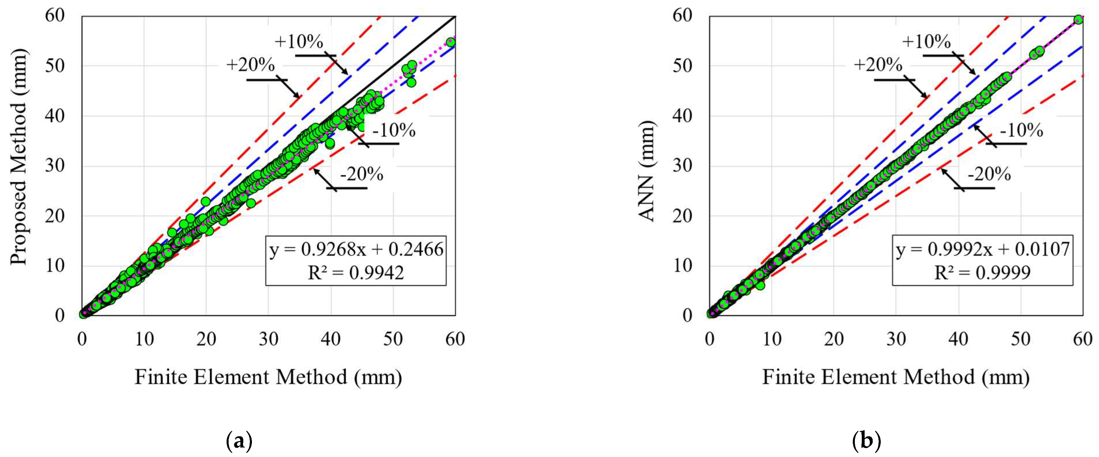
7. Comparative Study

The statistical analysis reveals, as shown in Figure 11, that the proposed method reached 80.8% in terms of observations, indicating safety with a $w_{proposed}/w_{FEM}$ ratio < 1.0. The maximum and minimum relative errors ($w_{proposed}/w_{FEM}$ − 1) for this method were 16% and −30%, respectively. In contrast, the ANN model demonstrated higher accuracy, with maximum and minimum relative errors of 33% and −25%.

Table 8. Statistical analysis of comparative study.

Model	Proposed	ANN
Mean	0.95	1.00
S.D	7.15%	2.79%
R2	0.9942	0.9999
MAE	0.904	0.087
RMSE	1.550	0.154
Minimum error (WPredicted/NFE − 1)	−30%	−25%
Maximum error (WPredicted/NFE − 1)	16%	33%

summarizes the statistical results, indicating that both models are suitable for practical applications and design purposes.

8. Benchmarking the Proposed Analytical Method Against SCI P355 and FEM

As explained previously, the literature currently lacks studies on the deflection calculations for cellular beams with tapered sections; most existing works focus solely on beams with constant sections. The proposed formulation addresses this gap by incorporating a parameter ($\alpha$) that accounts for all web height dimensions, including prismatic sections.

In this section, we validate the proposed formulation for cellular beams with a constant web section ($\alpha =1$) by comparing its predictions to those obtained via finite element modelling and the standard SCI P355 code. The comparison includes total elastic deflections ($w$), additional deflections ($w_{add}$) computed using the proposed formulation, Abaqus/CAE 2017 FEM results ($w_{FEM}$), and deflections derived from SCI P355 through Equation (2).

Five IPE beam are analysed for simply supported beams subjected to two load cases: three-point bending and four-point bending. The geometrical properties of the beams studied in this comparison are presented in

Table 9. Geometries of cellular steel beams used in comparison.

Beam	tf [mm]	tw [mm]	b [mm]	h [mm]	Openings	D [mm]	W [mm]	P [mm]	L [m]
B1	19	12	220	600	14	257.6	125	382.6	6
B2	19	12	220	600	24	161.6	80	241.6	6
B3	16	10.2	200	745	10	525	135	660	7
B4	16	10.2	200	745	13	525	135	660	9
B5	19	12	220	896	11	630	160	790	9

. It is also important to note that concentrated forces are applied to the upper flange of the beams for each load case.

The relative errors associated with the proposed method—$w$, $w_{(SCI P355)}$, and $w_{FEM}$—are given respectively by the expressions (35) and (36). The comparison results are listed in

Table 10. Total deflection of prismatic cellular steel beams ($\alpha$ = 1) under two load cases.

Beam	Load case	P [kN]	${\mathit{w}}_{\mathit{a}\mathit{d}\mathit{d}}$ [mm]	${\mathit{w}}_0$ [mm]	$\mathit{w}$ [mm]	SCI P355 [mm]	${\mathit{w}}_{\left(\mathit{S}\mathit{C}\mathit{I}\mathit{P}355\right)}$ [mm]	${\mathit{w}}_{\mathit{F}\mathit{E}\mathit{M}}$ [mm]	${\mathsf{\Delta }}_1$ (%)	${\mathsf{\Delta }}_2$ (%)
B1	3 pts	100	0.50	2.43	2.92	0.129	2.74	3.33	12.25	17.71
B2	3 pts	100	0.37	2.43	2.79	0.087	2.64	3.14	11.08	15.99
B3	3 pts	100	2.886	2.937	5.82	0.260	3.70	5.78	0.76	35.98
B4	3 pts	100	3.464	6.242	9.71	0.262	7.88	10.12	4.09	22.13
B5	3 pts	100	2.43	3.230	5.66	0.266	4.09	6.14	7.88	33.47
B1	4 pts	50	0.28	1.67	1.95	0.129	1.88	2.16	9.68	12.78
B2	4 pts	50	0.18	1.67	1.85	0.087	1.81	2.04	9.27	11.10
B3	4 pts	50	1.732	2.019	3.75	0.260	2.54	3.39	10.66	24.97
B4	4 pts	50	1.732	4.292	6.02	0.262	5.42	6.21	2.98	12.74
B5	4 pts	50	1.458	2.220	3.68	0.266	2.81	3.74	1.54	24.78

.

$${\mathrm{\Delta }}_1={\displaystyle \frac{\left|w-w_{FEM}\right|}{w_{FEM}}}\times 100$$

(35)

$${\mathrm{\Delta }}_2={\displaystyle \frac{\left|w_{\left(SCI P355\right)}-w_{FEM}\right|}{w_{FEM}}}\times 100$$

(36)

Table 10 clearly shows that the validation process was very successful. In the first phase, the proposed method aligns well with the Finite Element Method (FEM) results, with relative errors (${\mathrm{\Delta }}_{₁}$) ranging from 0.76% to 12.25%. These small errors indicate that the analytical method is both robust and reliable, particularly in how accurately it calculates the additional deflection of cellular steel beams.

In the second part of the comparison, the relative error (${\mathrm{\Delta }}_2$) between the deflection values predicted by the SCI P355 formulation and those from the FEM for cellular steel beams with constant sections was significantly larger, ranging from 11.1% to 35.98%. This highlights the fact that the SCI P355 formulation, although useful in some situations, tends to underestimate the total deflection of cellular steel beams. The SCI P355 method fails to fully account for the complexities introduced by variations in geometry and local shear forces, which further emphasizes the need for a more detailed and accurate analytical approach.

Additional validation tests were not deemed necessary, as they showed similar results, reinforcing the initial findings. These discrepancies underscore the importance of developing methods that better capture the complexity of cellular steel beams, including their local variations and the impact of shear forces.

The method works by evaluating the additional deflection for each opening individually, considering the specific geometry of each T-section formed by the web and flanges of the beam. Additionally, the exact shear force ($V$) acting on each T-section is included in the calculation. This shear force can vary across the length of the beam, depending on both the type of global loading and the position of the openings, which makes the method highly precise and well suited for handling changes in geometry and local load distributions. The overall additional deflection is then obtained by summing the contributions from each opening. To streamline the process, a MATLAB R2019a program was developed to help automate the calculations, making this approach practical for real-world applications. This thorough approach ensures an accurate and reliable model of the structural behaviour of the beam.

Ultimately, it is clear that the SCI P355 formulation underestimates the total deflection of cellular steel beams. On the other hand, the proposed method delivers highly accurate results that align closely with the FEM predictions. This precision, combined with the detailed consideration of geometric variations and local forces, makes the method an excellent tool for structural design.

In conclusion, the comparison highlights the clear advantage of the proposed analytical method for predicting the deflections of cellular steel beams under different loading conditions and geometries. By addressing the limitations of SCI P355, the method fills an important gap in current design practices and provides engineers with a more reliable and accurate solution.

9. Conclusions

This paper presents both analytical and artificial neural network (ANN) solutions to predict the additional and total deflection of tapered cellular steel beams under various loading conditions, including three-, four-, and five-point bending, as well as cantilever loading. The proposed method is based on Vierendeel beam behaviour, calculating additional deflection by considering shear and bending effects on circular web openings, with equal transverse displacement assumed in the upper and lower tee-sections. A new parameter ($\alpha$) is introduced to represent the tapered geometry factor in non-prismatic beams, which is used to estimate deflections. The results showed good agreement with the finite element models, with additional deflection being more significant in beams with fewer web openings. As the tapered section factor increases, additional deflection decreases, though its impact grows with higher tapered section values. The ANN-based formula using six neurons accurately predicted deflections and is suitable for design purposes, particularly for the Service Limit State. The proposed analytical method provides a highly precise and computationally efficient alternative to finite element simulations for non-prismatic beams, with error margins significantly lower than those observed in the SCI P355 code. Future studies could further explore the applicability of the analytical model for beams with non-circular openings or under dynamic loading conditions.

References

1. Boissonnade, N.; Muzeau, J.-P. Mise au Point d’un Elément fini de Type Poutre à Section Variable et Autres Applications à la Construction Métallique. 2002. Available online: https://theses.fr/2002CLF21394 (accessed on 15 March 2025).
2. Hosain, M.U.; Speirs, W.G. Experiments on Castellated Steel Beams; Welding Research Supplement; Department of Civil Engineering, University of Saskatchewan: Saskatoon, SK, Canada, 1973; pp. 329–342. [Google Scholar]
3. Ferreira, F.P.V.; Rossi, A.; Martins, C.H. Lateral-torsional buckling of cellular beams according to the possible updating of EC3. J. Constr. Steel Res. 2019, 153, 222–242. [Google Scholar] [CrossRef]
4. Ferreira, F.P.V.; Shamass, R.; Santos, L.F.P.; Tsavdaridis, K.D.; Limbachiya, V. Web-post buckling resistance calculation of perforated high-strength steel beams with elliptically-based web openings for EC3. Structures 2023, 55, 245–262. [Google Scholar] [CrossRef]
5. BS EN 1993.1.1:2022; Eurocode 3—Design of Steel Structures. Part 1-1: General Rules and Rules for Buildings. British Standards: London, UK, 2022.
6. BS EN 1993-1-13; Eurocode 3. Design of Steel Structures. Beams with Large Web Openings. British Standards: London, UK, 2024.
7. Lawson, R.M.; Hicks, S.J. Design of Composite Beams with Large Web Openings, P355 ed.; The Steel Construction Institute: London, UK, 2011. [Google Scholar]
8. Fares, S.S.; Coulson, J.; Dinehart, D.W. AISC Steel Design Guide 31: Castellated and Cellular Beam Design; American Institute of Steel Construction: Chicago, IL, USA, 2016. [Google Scholar]
9. Thai, H.T. Machine learning for structural engineering: A state-of-the-art review. Structures 2022, 38, 448–491. [Google Scholar] [CrossRef]
10. Shamass, R.; Ferreira, F.P.V.; Limbachiya, V.; Santos, L.F.P.; Tsavdaridis, K.D. Web-post buckling prediction resistance of steel beams with elliptically-based web openings using Artificial Neural Networks (ANN). Thin-Walled Struct. 2022, 180, 109959. [Google Scholar] [CrossRef]
11. Gholizadeh, S.; Pirmoz, A.; Attarnejad, R. Assessment of load carrying capacity of castellated steel beams by neural networks. J. Constr. Steel Res. 2011, 67, 770–779. [Google Scholar] [CrossRef]
12. Sharifi, Y.; Tohidi, S. Lateral-torsional buckling capacity assessment of web opening steel girders by artificial neural networks—Elastic investigation. Front. Struct. Civ. Eng. 2014, 8, 167–177. [Google Scholar] [CrossRef]
13. Tohidi, S.; Sharifi, Y. Neural networks for inelastic distortional buckling capacity assessment of steel I-beams. Thin-Walled Struct. 2015, 94, 359–371. [Google Scholar] [CrossRef]
14. Tohidi, S.; Sharifi, Y. Load-carrying capacity of locally corroded steel plate girder ends using artificial neural network. Thin-Walled Struct. 2016, 100, 48–61. [Google Scholar] [CrossRef]
15. Hosseinpour, M.; Sharifi, Y.; Sharifi, H. Neural network application for distortional buckling capacity assessment of castellated steel beams. Structures 2020, 27, 1174–1183. [Google Scholar] [CrossRef]
16. Nguyen, T.-A.; Ly, H.-B.; Tran, V.Q. Investigation of ANN Architecture for Predicting Load-Carrying Capacity of Castellated Steel Beams. Complexity 2021, 2021, 6697923. [Google Scholar] [CrossRef]
17. Abambres, M.; Rajana, K.; Tsavdaridis, K.; Ribeiro, T. Neural Network-Based Formula for the Buckling Load Prediction of I-Section Cellular Steel Beams. Computers 2018, 8, 2. [Google Scholar] [CrossRef]
18. Ferreira, F.P.V.; Shamass, R.; Limbachiya, V.; Tsavdaridis, K.D.; Martins, C.H. Lateral–torsional buckling resistance prediction model for steel cellular beams generated by Artificial Neural Networks (ANN). Thin-Walled Struct. 2022, 170, 108592. [Google Scholar] [CrossRef]
19. Rabi, M.; Jweihan, Y.S.; Abarkan, I.; Ferreira, F.P.V.; Shamass, R.; Limbachiya, V.; Tsavdaridis, K.D.; Santos, L.F.P. Machine learning-driven web-post buckling resistance prediction for high-strength steel beams with elliptically-based web openings. Results Eng. 2024, 21, 101749. [Google Scholar] [CrossRef]
20. Degtyarev, V.V.; Tsavdaridis, K.D. Buckling and ultimate load prediction models for perforated steel beams using machine learning algorithms. J. Build. Eng. 2022, 51, 104316. [Google Scholar] [CrossRef]
21. Dassault Systèmes. ABAQUS 2017 Documentation. 2017. Available online: https://www.3ds.com/products-services/simulia/products/abaqus/ (accessed on 15 March 2025).
22. BS EN 1994-1-1:2004; Eurocode 4: Design of Steel and Concrete Composite Structures. Part 1.1: General Rules and Rules for Buildings. British Standards: London, UK, 2004.
23. Lawson, R.M. Design for Openings in the Webs of Composite Beams; CIRIA: London, UK, 1987. [Google Scholar]
24. Lawson, R.M.; Chung, K.F.; Price, A.M. Tests on composite beams with large web openings to justify existing design methods. Struct. Eng. Lond. 1992, 70, 1–7. [Google Scholar]
25. Lawson, R.M.; Lim, J.; Hicks, S.J.; Simms, W.I. Design of composite asymmetric cellular beams and beams with large web openings. J. Constr. Steel Res. 2006, 62, 614–629. [Google Scholar] [CrossRef]
26. Ward, J.K. Design of Composite and Non-Composite Cellular Beams. 1990. Available online: https://www.abebooks.com/9781870004510/Design-Composite-Non-composite-Cellular-Beams-1870004515/plp (accessed on 15 March 2025).
27. Redwood, R.G. Design of Beams with Web Holes; Canadian Steel Industries Construction Council: Markham, ON, Canada, 1973. [Google Scholar]
28. Tsavdaridis, K.D. Structural Performance of Perforated Steel Beams with Novel Web Openings and with Partial Concrete Encasement. Ph.D. Thesis, City University London, London, UK, 2010. [Google Scholar]
29. MathWorks. MATLAB R2019a Documentation. 2019. Available online: https://www.mathworks.com (accessed on 15 March 2025).
30. Osmani, A.; Meftah, S.A. Lateral buckling of tapered thin walled bi-symmetric beams under combined axial and bending loads with shear deformations allowed. Eng. Struct. 2018, 165, 76–87. [Google Scholar] [CrossRef]
31. Saoula, A.; Meftah, S.A.; Mohri, F.; Daya, E.M. Lateral buckling of box beam elements under combined axial and bending loads. J. Constr. Steel Res. 2016, 116, 141–155. [Google Scholar] [CrossRef]
32. Benyamina, A.B.; Meftah, S.A.; Mohri, F.; Daya, E.M. Analytical solutions attempt for lateral torsional buckling of doubly symmetric web-tapered I-beams. Eng. Struct. 2013, 56, 1207–1219. [Google Scholar] [CrossRef]
33. Moradi, M.J.; Khaleghi, M.; Salimi, J.; Farhangi, V.; Ramezanianpour, A.M. Predicting the compressive strength of concrete containing metakaolin with different properties using ANN. Measurement 2021, 183, 109790. [Google Scholar] [CrossRef]
34. Jin, J.; Li, M.; Jin, L. Data Normalization to Accelerate Training for Linear Neural Net to Predict Tropical Cyclone Tracks. Math. Probl. Eng. 2015, 2015, 931629. [Google Scholar] [CrossRef]
35. Olden, J.D.; Jackson, D.A. Illuminating the “black box”: Understanding variable contributions in artificial neural networks. Ecol. Modell. 2002, 154, 135–150. [Google Scholar] [CrossRef]
36. Limbachiya, V.; Shamass, R. Application of Artificial Neural Networks for web-post shear resistance of cellular steel beams. Thin-Walled Struct. 2021, 161, 107414. [Google Scholar] [CrossRef]
37. Garson, D.G. Interpreting neural network connection weights. AI Expert 1991, 6, 46–51. [Google Scholar]
38. Gupta, T.; Patel, K.A.; Siddique, S.; Sharma, R.K.; Chaudhary, S. Prediction of mechanical properties of rubberised concrete exposed to elevated temperature using ANN. Measurement 2019, 147, 106870. [Google Scholar] [CrossRef]
39. Sharifi, Y.; Moghbeli, A. Shear capacity assessment of steel fiber reinforced concrete beams using artificial neural network. Innov. Infrastruct. Solut. 2021, 6, 89. [Google Scholar] [CrossRef]
40. al-Swaidani, A.M.; Khwies, W.T. Applicability of Artificial Neural Networks to Predict Mechanical and Permeability Properties of Volcanic Scoria-Based Concrete. Adv. Civ. Eng. 2018, 2018, 5207962. [Google Scholar] [CrossRef]
41. Tsavdaridis, K.D.; D’Mello, C. Web buckling study of the behaviour and strength of perforated steel beams with different novel web opening shapes. J. Constr. Steel Res. 2011, 67, 1605–1620. [Google Scholar] [CrossRef]
Figure 2. Schematic representation of additional deflection due to web openings in tapered cellular steel beams.
Buildings 15 00992 g002
Figure 3. Details of the cellular beam for the program.
Buildings 15 00992 g003
Figure 4. Boundary conditions of considered tapered cellular steel beam.
Buildings 15 00992 g004
Figure 5. Loading conditions considered for the tapered cellular steel beam. (a) Three-point bending; (b) four-point bending; (c) five-point bending; (d) cantilever.
Buildings 15 00992 g005
Figure 6. Proposed ANN framework considering 8 neurons. (a) Three-point bending; (b) four-point bending; (c) five-point bending; (d) cantilever.
Buildings 15 00992 g006
Figure 7. Influence of additional deflection on total deflection considering IPE 600 section. (a) Three-point bending; (b) four-point bending; (c) five-point bending; (d) cantilever.
Buildings 15 00992 g007aBuildings 15 00992 g007b
Figure 8. Total deflection vs. number of openings considering IPE 600 section. (a) Three-point bending; (b) four-point bending; (c) five-point bending; (d) cantilever.
Buildings 15 00992 g008aBuildings 15 00992 g008b
Figure 9. Variable contributions, dimensions in mm. (a) Three-point bending; (b) four-point bending; (c) five-point bending; (d) cantilever.
Buildings 15 00992 g009
Figure 10. Impact of input parameters, dimensions in mm. (a) Three-point bending; (b) four-point bending; (c) five-point bending; (d) cantilever.
Buildings 15 00992 g010
Figure 11. Comparative analyses for actual and predicted values using analytical method and ANN. (a) Analytical method; (b) ANN−based method.
Buildings 15 00992 g011