Research on Quasi-Elastic–Plastic Optimization of Reinforced Concrete Frame–Shear Wall Structures

Abstract

Precise determination of structural elastic–plastic displacement and component states under rare earthquakes is crucial for structural design. This article proposes a quasi-elastic–plastic optimization method for reinforced concrete structures. First, an approximate formula for calculating the yield bending moment of shear walls is provided through analysis of 64 shear walls. Second, a quasi-elastic–plastic analysis method is proposed. Using the elastic response spectrum analysis, strain energy for each component is calculated, and stiffness reduction factors for walls, beams, and columns are derived based on the energy equivalence principle. Finally, combining the elastic response spectrum analysis and the quasi-elastic–plastic analysis, various constraint indicators at the elastic and elastic–plastic design stages are calculated, and structural size optimization is completed using the particle swarm optimization method. The feasibility of this method is validated with examples of a 15-story reinforced concrete frame structure and a 15-story frame–shear wall structure. The quasi-elastic–plastic optimization with the particle swarm optimization efficiently completes elastic–plastic optimization for reinforced concrete structures, determining section sizes that meet performance standards while reducing material usage.

1. Introduction

Under the action of a major earthquake, structures may enter an elastic–plastic state. Achieving and enhancing the elastic–plastic performance of structures is a critically important topic. The elastic–plastic performance of a structure can be improved through various approaches, such as adjusting structural layout, optimizing component dimensions, and selecting different materials. Currently, for structures with determined topology, component dimensions, and materials, the analysis of their elastic–plastic performance can generally be conducted through the following methods:

Nonlinear static analysis methods, ranging from single fixed loading patterns [1] to multi-mode pushover methods [2,3] and higher-order modal pushover methods [4,5,6], cannot directly reflect the sequence of structural damage development. Some researchers have proposed adaptive pushover methods based on force or displacement, which update the lateral force distribution patterns during the damage progression process to better represent damage development [7,8,9]. However, these methods require substantial computational effort and time, making them challenging to apply in all engineering cases. Furthermore, they are not particularly effective in predicting the deformation modes of buildings. The Incremental Dynamic Analysis (IDA) method represents an extension of the dynamic time–history analysis approach. It enables systematic investigation of structural seismic performance by establishing correlation curves between structural damage indices and seismic intensity measures, thereby comprehensively reflecting the entire damage accumulation and failure process under earthquake excitation [10]. Tang [11] implemented an IDA-based seismic fragility assessment methodology to evaluate the seismic vulnerability of long-span spatial structures. Liu [12] proposed a failure mode regulation strategy for primary–secondary structural systems through degradation-controllable bracing elements, based on the principle of rational seismic failure sequence. Although dynamic time–history analysis-based methods can accurately capture structural internal forces and displacements under seismic actions, refined modeling and nonlinear analysis of structural systems still entail a substantial computational overhead.

The pseudo-elastoplastic method (equivalent linearization method) approximates seismic displacement responses of nonlinear structures by establishing equivalent linear elastic models with stiffness reduction and damping enhancement. Gulkan and Sozen [13] demonstrated that employing the secant period as the equivalent linear period enables non-conservative prediction of maximum displacements in inelastic systems. Building upon this foundation, Akimori Shibata [14,15] developed the “equivalent structural method”, which constructs equivalent multi-degree-of-freedom elastic systems through adjustments in component stiffness matrices and equivalent damping ratios. Yoshida [16] subsequently modified this approach for the seismic response verification of existing structures. Lin and Miranda [17,18] established computational criteria for equivalent period and damping ratio based on strength ratio definitions to determine post-yield maximum responses in single-degree-of-freedom systems. Wang and Hua [19] approximated nonlinear restoring forces as bilinear forms while evaluating linearization errors. Guyader [20] proposed a two-dimensional search algorithm to optimize equivalent period and damping ratio solutions, thereby deriving equivalent structural stiffness. Samimifar and Massumi [21] developed an equivalent linear analysis model that equates maximum seismic-induced displacements to hysteretic energy-equivalent displacements of nonlinear systems, simplifying computation by equivalating nonlinear seismic energy to the area under linear force–displacement curves. However, current research exhibits three primary limitations: 1. Existing studies predominantly focus on equivalent linearization analysis of beam–column components, with limited investigation on shear wall elements. 2. The applicability of these methods to large-scale reinforced concrete structures remains undemonstrated, as current validations concentrate on simple structural configurations. 3. Few documented studies have yet explored the application of equivalent linearization analysis to structural optimization.

In response to the issue of multiple iterations being required during the elastoplastic optimization process, and that the time-consuming nature of time–history analysis is unacceptable, along with the limited research on the calculation methods for shear wall yield bending moments, this article proposes a quasi-elastic–plastic optimization method for reinforced concrete structures. Based on the energy equivalence principle, stiffness reduction factors are applied to walls, beams, and columns, establishing a quasi-elastic–plastic analysis approach. By combining the quasi-elastic–plastic analysis method with intelligent optimization algorithms, the optimization of reinforced concrete structural cross-sectional dimensions is achieved with performance indicators from both the elastic design phase and the elastic–plastic design phase as constraints, and structural cost as the optimization objective. Considering that the particle swarm optimization (PSO) algorithm exhibits good convergence speed in high-dimensional spaces [22], the PSO is adopted as the optimization algorithm in this study. A dedicated optimization program was developed in C++ using ETABS for structural analysis. Validation through a frame structure and a frame–shear wall structure, compared against nonlinear time–history analysis, confirmed the accuracy and suitability of the method, achieving efficient elastic–plastic optimization that is challenging to accomplish using time–history analysis.

2. Yield Bending Moment of Reinforced Concrete Component

The calculation of component yield bending moments significantly impacts the energy equivalence process in quasi-elastic–plastic analysis, as over- or underestimating these values can cause theoretical deformation to deviate from actual deformation. For calculating the yield bending moment of concrete member cross-sectional capacity, the following basic assumptions are made [23]:

(1) The deformed cross-section remains planar and perpendicular to the neutral axis. (2) Concrete tensile strength is neglected. (3) The stress ${\sigma }_c$ and strain ${\epsilon }_c$ relationship for compressed concrete is as follows:

$${\sigma }_c=\left\{\begin{array}{l}{f}_c\left[1-{\left(1-{\displaystyle \frac{{\epsilon }_c}{{\epsilon }_0}}\right)}^n\right]\hspace{1em}\hspace{1em}{\epsilon }_c\le {\epsilon }_0\\ f_c\hspace{1em}\hspace{1em}\hspace{1em}\hspace{1em}\hspace{1em}\hspace{1em}\hspace{1em}\hspace{1em} {\epsilon }_0<{\epsilon }_c\le {\epsilon }_{cu}\end{array}\right.$$

(1)

where $f_c$ is the design compressive strength; ${\epsilon }_0$ is the strain at compressive stress $f_c$; ${\epsilon }_{cu}$ is the ultimate compressive strain; and $n$ is a coefficient determined by the standard compressive strength of concrete cubes. (4) The stress ${\sigma }_s$ of longitudinal reinforcement equals the product of elastic modulus $E_s$ and reinforcement strain ${\epsilon }_s$, i.e., ${\sigma }_s=E_s·{\epsilon }_s\le f_y$, where $f_y$ is the ultimate tensile strain of the longitudinal reinforcement.

The yield bending moments of beams and columns can be referenced in the literature [23]. The failure modes of shear walls may be bending, shear, bending–shear, and other types of failure [24,25]. Shear walls play a critical role in the structure and should be designed to fail in bending rather than in shear [23]; therefore, this study assumes that shear walls follow bending failure, and the yield bending moment of shear walls is calculated based on the nominal strength of the cross-section.

The stress and strain distribution of the rectangular shear wall section with symmetric reinforcement at yield state is shown in Figure 1. Based on the plane section assumption and equilibrium conditions, the yield bending moment $M_y$ of the shear wall can be expressed as follows:

$$\begin{array}{c}{M}_y=F_s\left(h_w-l_c\right)/2+F_{sw}\left(1/6h_w-2/3a_s+1/3x\right)+F_s^{\prime }\left(h_w-l_c\right)/2+\\ F_{sw}^{\prime }\left(1/2h_w-2/3a_s^{\prime }-1/3x\right)+F_c\left(1/2h_w-1/3x\right)\end{array}$$

(2)

where $F_s$ represents the resultant force of the longitudinal tensile reinforcement in the confined boundary elements. $F_{sw}$ represents the resultant force of the vertical distributed reinforcement in the tensile zone. $F_s^{\prime }$ represents the resultant force of the longitudinal compressive reinforcement in the confined boundary elements. $F_{sw}^{\prime }$ represents the resultant force of the vertical distributed reinforcement in the compressive zone. $F_c$ represents the resultant force of the concrete in the compressive zone. $E_c$ is the elastic modulus of the concrete material. $h_w$ is the height of the wall cross-section. $l_c$ the length of the confined boundary elements along the wall limb. $a_s^{\prime }$ is the thickness of the concrete cover in the compressive zone. $a_s$ is the thickness of the concrete cover in the tensile zone. $x$ is the height of the compressive zone.

From Equation (2), it can be seen that the yield bending moment of the shear wall is primarily influenced by the section height, edge components, distributed reinforcement, and the height of the compressive zone. However, calculating the height of the compressive zone is complex and difficult to express with a formula. Ji [26] studied the mechanical performance of reinforced concrete shear walls with medium shear span-to-depth ratios, which has some discrepancies with the calculation results from the standard [27]. The author also investigated the performance of shear walls with low shear span-to-depth ratios [28]. In this chapter, it is assumed that the yield mode of the shear wall is due to the yielding of the edge component reinforcement in tension. A total of 64 shear wall samples were established, and the yield bending moment under different axial forces, section heights, vertical reinforcement ratios, and edge component tensile reinforcement areas was calculated using XTRACT. The calculation results are shown in

Table 1. Parameter table of shear wall samples for fitting.

SWSD (mm)	VR	BER	AI (kN)	XBM (kN·m)	SWSD (mm)	VR	BER	AI (kN)	XBM (kN·m)
200 × 1500	C8@150	6 C18	0	914	200 × 2500	C8@150	6 C16	0	1632
			1000	1455				1000	2638
			2000	1853				2000	3525
			3000	2045				3000	4270
		6 C16	0	755			6 C14	0	1383
			1000	1311				1000	2401
			2000	1715				2000	3289
			3000	1900				3000	4036
	C6@150	6 C18	0	933		C6@150	6 C16	0	1559
			1000	1458				1000	2587
			2000	1983				2000	3488
			3000	2508				3000	4248
		6 C16	0	730			6 C14	0	1115
			1000	1276				1000	2158
			2000	1713				2000	3094
			3000	2010				3000	3884
200 × 2000	C8@150	6 C16	0	1132	200 × 3000	C8@150	6 C18	0	2392
			1000	1920				1000	3627
			2000	2592				2000	4764
			3000	3058				3000	5776
		6 C14	0	939			6 C16	0	2045
			1000	1738				1000	3281
			2000	2412				2000	4418
			3000	2877				3000	6243
	C6@150	6 C16	0	1061		C6@150	6 C18	0	2201
			1000	1843				1000	3449
			2000	2525				2000	4602
			3000	3061				3000	5611
		6 C14	0	859			6 C16	0	1841
			1000	1666				1000	3118
			2000	2344				2000	4269
			3000	2883				3000	5283

Ps: SWSD is the shear wall section dimension; VR is the vertical reinforcement; BER is the boundary element reinforcement; AI is the axial load; XBM is the XTRACT bending moment.

. Using OriginPro 2021 software, an approximate formula for the yield bending moment $M_{y,f}$ of the shear wall is derived, as shown in Equation (3).

$$M_{y,f}=f_y{A}_s{h}_w+0.37 N{h}_w+0.25 f_y{\rho }_w{b}_w{h}_w^2$$

(3)

where $A_s$ is the reinforcement area of the boundary element, ${\rho }_w$ is the vertical reinforcement ratio, $b_w$ is the wall thickness, and $N$ is the axial load on the shear wall. The remaining symbols are defined in the relevant descriptions of Equations (1) and (2). The yield bending moment of a shear wall is related to its cross-sectional area, reinforcement ratio, and the horizontal dimensions of the section, with the length of the shear wall having a greater impact. Substituting the parameter values of each shear wall sample from Table 1 into Equation (3), the calculation results were compared with the values obtained from XTRACT, as shown in Figure 2. For the selected samples, the average error of the fitted formula compared to the XTRACT results is approximately 9%.

3. Quasi-Elastic–Plastic Optimization of Reinforced Concrete Structures

3.1. Quasi-Elastic–Plastic Analysis Method for Reinforced Concrete Structures

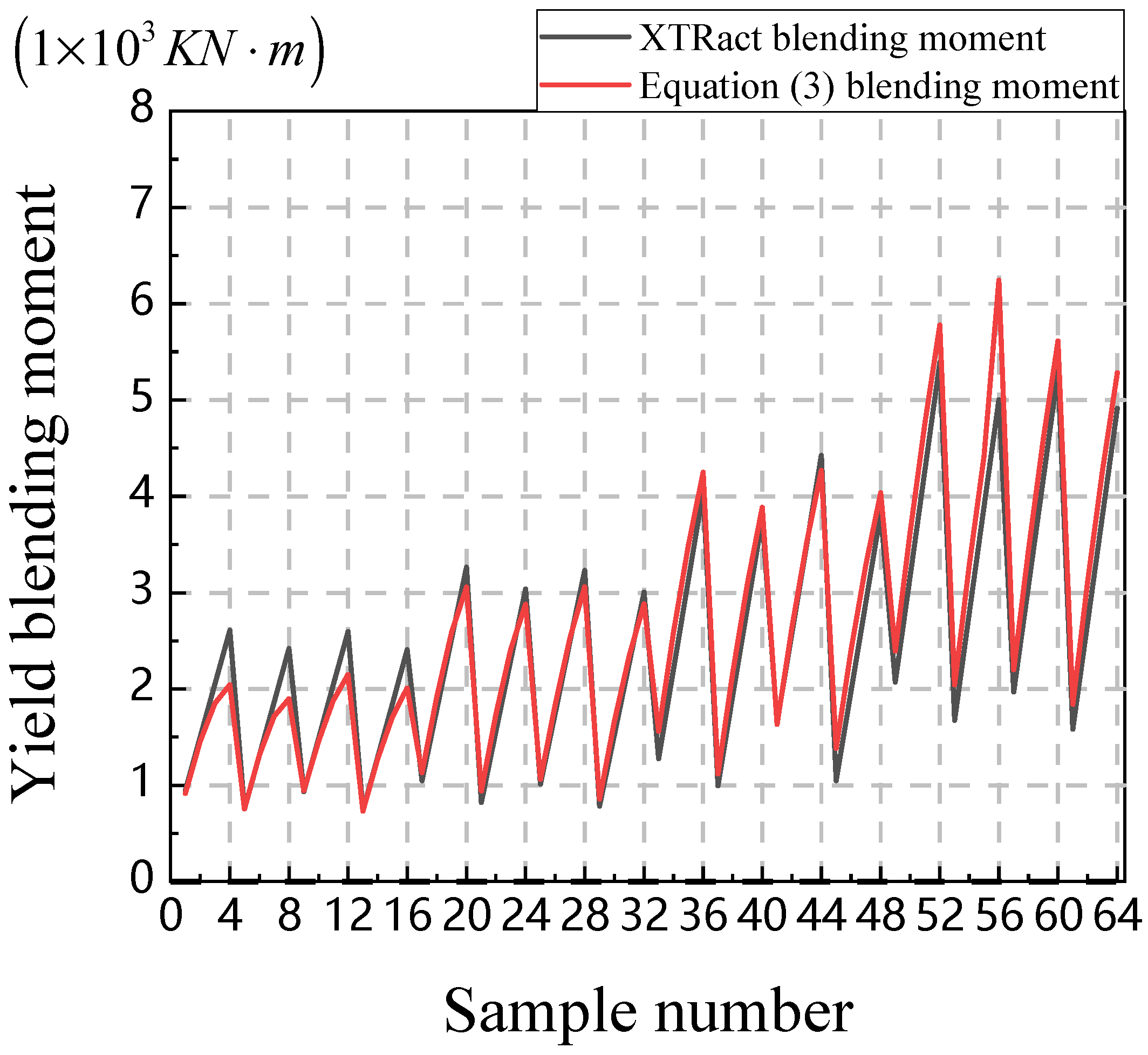
Assume that the structure remains in an elastic state. Through elastic analysis, the maximum bending moment of the structural member section under rare earthquake loads can be obtained. According to the equal energy criterion proposed by Veletsos and Newmark [29], under the maximum response displacement, the maximum potential energy of the elastic system and the elastoplastic system are equal. Herein, the equivalent stiffness of the structural member in the elastoplastic state is calculated to obtain the stiffness reduction factor of the member.

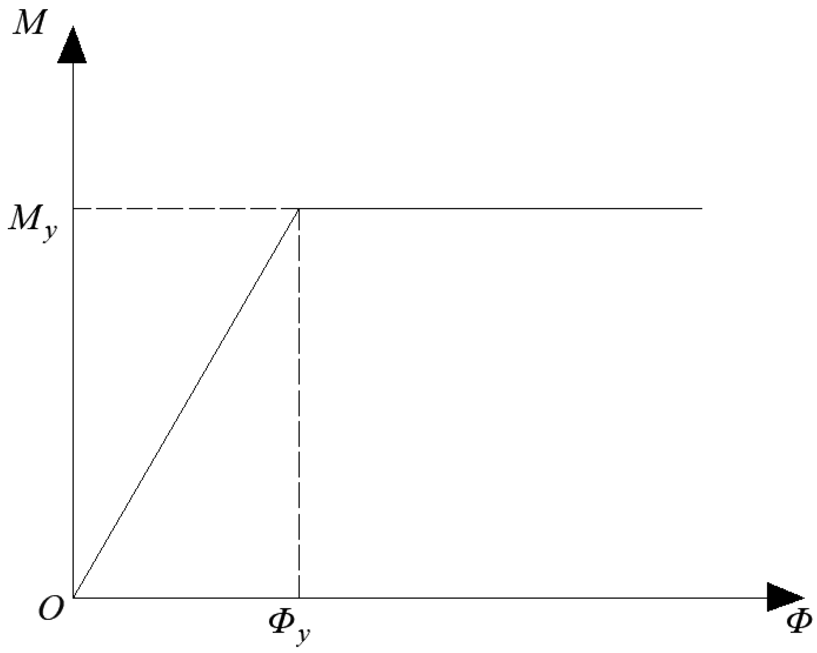
The moment–rotation model of the reinforced concrete member is simplified to a bilinear model, assuming that the curve remains horizontal after the member yields. The moment–rotation curve of the ideal elastoplastic member is shown in Figure 3, and the energy equivalence process is shown in Figure 4. $M_y$ is the yield bending moment of the member; ${\mathsf{\Phi }}_y$ is the yield rotation of the member; $M_{c,i}$ is the bending moment of the member calculated using the elastic method during the $i$-th iteration; ${\mathsf{\Phi }}_{c,i}$ is the elastic rotation of the member during the $i$-th iteration; ${\mathsf{\Phi }}_{E,i}$ is the plastic rotation of the member during the $i$-th iteration; $k_{i-1}$ is the reduced stiffness of the member during the $i-1$-th iteration; and $k_i$ is the reduced stiffness of the member during the $i$-th iteration.

Based on the principle of equal strain energy [29], in both elastic and ideal elastoplastic states, the potential energy of structural components is equal, which can be represented as $SOAB=SOCDE$ as in Figure 4. Therefore, the limit state point $D$ and the corresponding rotation angle ${\mathsf{\Phi }}_{E,i}$ can be determined.

When $SOAB\le SOCG$, the component has not yielded, and $k_i=k_0$, where $k_0$ represents the initial stiffness of the component.

When $SOAB>SOCG$,

$${\displaystyle \frac{{M_{\mathrm{c},\mathrm{i}}}^2}{2k_{i-1}}}={\displaystyle \frac{{M_{\mathrm{y}}}^2}{2k_0}}+M_{\mathrm{y}}\left({\mathsf{\Phi }}_{E,i}-{\displaystyle \frac{M_{\mathrm{y}}}{k_0}}\right)$$

(4)

$${\mathsf{\Phi }}_{E,i}={\displaystyle \frac{M_{\mathrm{c},\mathrm{i}}^2}{2k_{i-1}{M}_{\mathrm{y}}}}+{\displaystyle \frac{M_{\mathrm{y}}}{2k_0}}$$

(5)

Assuming that the curvature of the component in the equivalent elastic state is equal to the curvature in the elastoplastic state, and based on the equivalence between the energy of the member in the ideal elastoplastic state and the energy corresponding to the maximum deformation under corrected stiffness in elastic analysis (i.e., $SOAB=SOEF$), the stiffness after elastoplastic deformation (i.e., $k_i$) can be determined.

$${\displaystyle \frac{{M_{\mathrm{c},\mathrm{i}}}^2}{2k_{i-1}}}={\displaystyle \frac{{{\mathsf{\Phi }}_{E,i}}^2{k}_i}{2}}$$

(6)

$$k_i={\displaystyle \frac{{M_{\mathrm{c},\mathrm{i}}}^2}{{{\mathsf{\Phi }}_{E,i}}^2{k}_{i-1}}}$$

(7)

The stiffness reduction factor ${\lambda }_i$ is defined as the ratio of the reduced stiffness to the initial elastic stiffness, as shown in Equation (8). The stiffness reduction factor reflects the current damage state of the component. If the component has not yielded, then ${\lambda }_i=1$.

$${\lambda }_i=k_i/k_0$$

(8)

Due to the stiffness reduction, the internal force distribution of the structure changes accordingly, leading to a variation in the stiffness reduction factors for the components based on the internal forces. Therefore, multiple iterations are required until convergence, ensuring that the stiffness reduction values of each component match their respective load conditions. In practical operations, the structural model should first be established, and the internal forces of the components should be calculated using the response spectrum method. Next, the stiffness reduction factors for each component are determined, followed by the reduction in the elastic modulus for each component based on these factors to obtain the equivalent model. This process is repeated for the equivalent model until convergence. In this way, the performance information of the structure after entering the elastoplastic state under rare seismic actions can be estimated under elastic analysis conditions. Finally, the automation of the proposed quasi-elastic–plastic analysis method was achieved based on the ETABS OAPI.

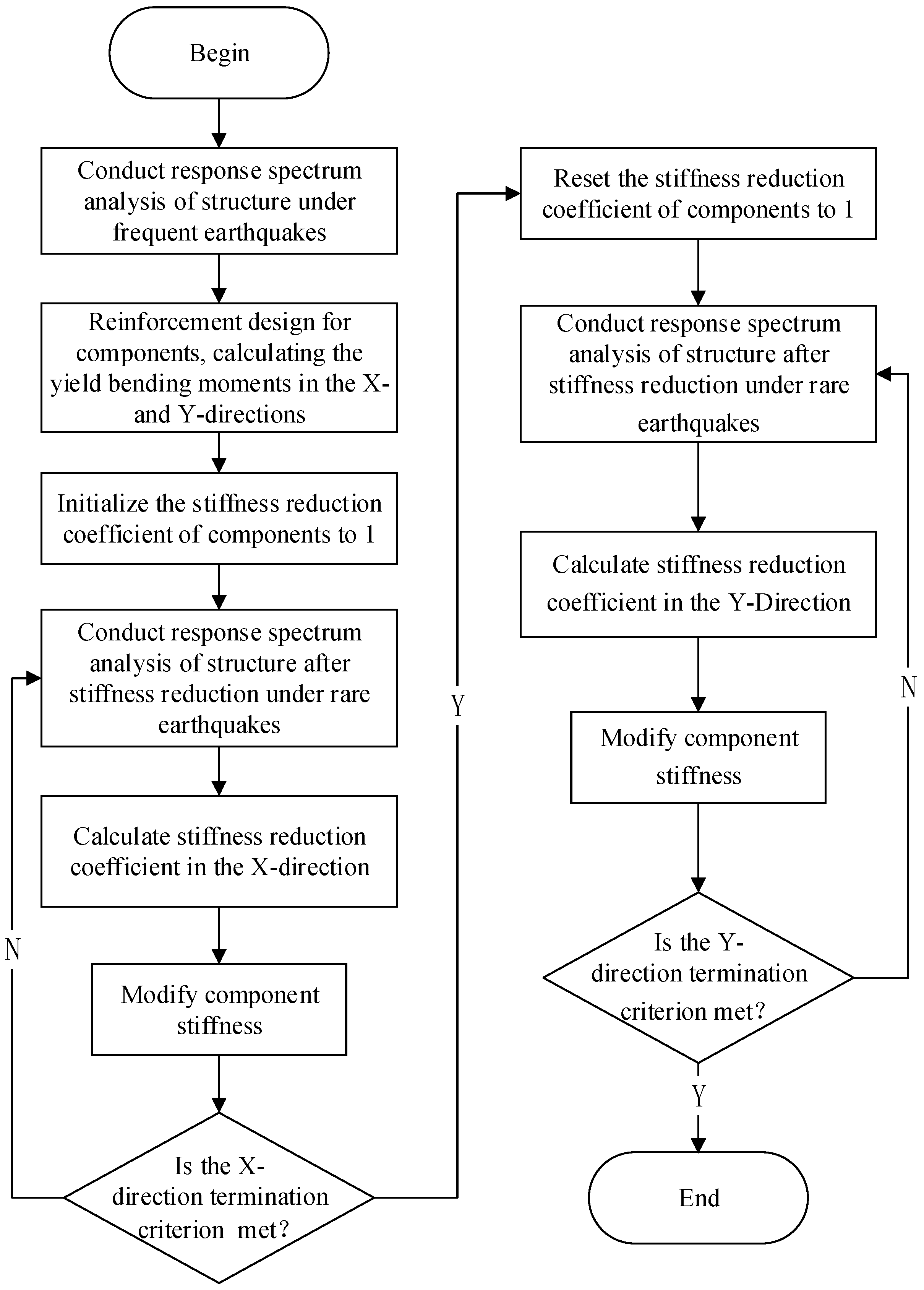
The flowchart of the proposed quasi-elastic–plastic analysis method is shown in Figure 5, and the specific process is as follows.

(1)

Calculate the frequent earthquake condition in the X-direction, complete the design of reinforcement for the components, and calculate the yield bending moment of each component.

(2)

Set the stiffness reduction factor for all components to 1.

(3)

Calculate the rare earthquake condition in the X-direction. Assume all components are elastic and use the elastic response spectrum method to calculate the maximum bending moment and axial force of each component under the condition of ‘1.0 dead load + 0.5 live load + seismic load’.

(4)

Calculate the stiffness reduction factor for each component. For components with bending moments exceeding the yield bending moment, reduce the stiffness by lowering the elastic modulus of the material and modify the structural model accordingly.

(5)

Repeat steps (2)–(5) until the termination criteria are met. The termination criterion is that the change in the stiffness reduction factor of all components between two consecutive iterations is less than 5%.

(6)

Initialize the structural model and calculate the seismic effects in the Y-direction using the same method.

3.2. Elastoplastic Optimization Model for Reinforced Concrete Frame–Shear Wall Structures

Based on the quasi-elastic–plastic analysis method for reinforced concrete structures, a quasi-elastic–plastic optimization method for reinforced concrete structures is introduced. The cross-sectional dimensions of beams, columns, and walls are used as variables, with the section numbers from the section library serving as the range of variable changes. The optimization design variables are defined as:

$$S={\{s_1,\cdots ,s_N\}}^T(l_n\le s_n\le u_n)$$

(9)

where $S$ represents the vector of section numbers; $s_n(n=1,\cdots ,N)$ represents the section number variables for the $n$-th group of components; $u_n$ and $l_n$ are the upper and lower limits of the section number for the $n$-th group of components, respectively. For the convenience of subsequent optimization, the section number vector $S$ is standardized according to Equations (10) and (11). In this chapter, the design variables do not include the reinforcement ratio of the components, as the reinforcement design is completed by ETABS according to the code requirements.

$$X={\{x_1,\cdots ,x_N\}}^T$$

(10)

$$x_n={\displaystyle \frac{s_n-l_n}{u_n-l_n}}$$

(11)

The optimization model can be obtained as follows:

$$\begin{array}{l}\mathrm{Objective} \mathrm{function}:W\left(X\right)=W\left(x_1,x_2,\dots ,x_N\right)\\ \mathrm{Constraint} \mathrm{function}:G_j\left(X\right)\le 0(j=1,2,\cdots ,15)\\ \mathrm{Range} \mathrm{of} \mathrm{variables}:l_n\le s_n\le u_n(n=1,2,\dots ,N)\end{array}$$

(12)

where $W$ is the cost of the structure, $X$ is the standardized vector; $G_j\left(X\right)(j=1,2,\cdots ,15)$ represents the structural performance constraint values that must be met during the elastic and elastoplastic design stages, and their calculation method is determined by Equation (13).

$$G_j(X)=\left\{\begin{array}{l}{\displaystyle \frac{P{I}_j}{{\mathrm{limit}}_j}}-1 \le 0 (j=1,\cdots ,7,14,15)\\ 1-{\displaystyle \frac{P{I}_j}{{\mathrm{limit}}_j}} \le 0 (j=8,\cdots ,13)\end{array}\right.$$

(13)

$G_j$ is the constraint value for the $j$-th structural performance indicator; $P{I}_j$ is the value of the $j$-th performance indicator, and ${\mathrm{limit}}_j$ is the limit value for the $j$-th performance indicator, as specified by the code [27]. The relationship between the names of performance indicators, their corresponding indicator numbers, and limit values is shown in

Table 2. The structural performance indicators considered in this study.

Performance Indicator	$\mathit{j}$	Limit
Story drift 1	1(X), 2(Y)	$\le 1/800$$, \le 1/550$
Displacement ratio	3(X), 4(Y)	$\le 1.5$
Interlayer displacement ratio	5(X), 6(Y)	$\le 1.5$
Period ratio	7	$\le 0.9$
Interlayer stiffness ratio 2	8(X), 9(Y)	$\ge 0.9$$,\ge 1.1$$,\ge 1.5$
Overturning stability factor 3	10(X), 11(Y)	$\ge 2.308$$,\ge 3$
Rigid weight ratio	12(X), 13(Y)	$\ge 1.4$
Elastoplastic interlayer displacement angle 4	14(X), 15(Y)	$\le 1/100,\le 1/50$

Ps: ¹ The limit values from left to right correspond to the frame–shear wall structure and the frame structure, respectively. ² The limit values from left to right are the general value, the value when the ratio of the height of the current floor to the height of the floor above is greater than 1.5, and the value when the story is a fixed base floor, respectively. ³ The limit values from left to right are for cases where the height-to-width ratio of the structure is no greater than 4, and for cases where the height-to-width ratio is greater than 4, respectively. ⁴ The limit values from left to right correspond to the frame–shear wall structure and the frame structure, respectively.

. The optimization objective is to obtain the component dimensions with the smallest $W$ value, while satisfying the performance indicators during the elastic design phase and the story drift constraints during the elastoplastic design phase.

3.3. Structural Dimension Optimization Process Based on Particle Swarm Optimization Method

Particle swarm optimization (PSO) is a heuristic algorithm inspired by the process of bird flocking and foraging. Through the exchange of information among multiple particles, all particles move towards better directions, gradually converging to the global optimum. In the PSO algorithm, particles can quickly adjust their search direction and speed by sharing information about their individual best positions and the global best position [30]. This allows them to move closer to better solutions, thereby achieving rapid convergence. In contrast, in the Genetic Algorithm (GA), there is less information exchange between individuals, which mainly rely on crossover and mutation operations to exchange information [31]. This method may lead to slower information propagation and affect the convergence speed. The fundamental principle of the PSO algorithm is as follows:

Let the number of variables be $NS$ and the number of particles be $NP$. In the $t$-th iteration step, the position vector $X_{np}^t$ and velocity vector ${\delta }_{np}^t$ of the $np$-th particle are given by Equations (14) and (15). Here, $x_{np,ns}^t$ and ${\delta }_{np,ns}^t(ns=1,\cdots ,NS)$ represent the $ns$-th component position and velocity, respectively. The position vector $X_{np}^{t+1}$ at time $t+1$ is obtained by the linear combination of $X_{np}^t$ and ${\delta }_{np}^{t+1}$, as shown in Equation (16).

$$X_{np}^t=\left(x_{np,1}^t,x_{np,2}^t,\cdots ,x_{np,NS}^t\right)$$

(14)

$${\delta }_{np}^t=\left({\delta }_{np,1}^t,{\delta }_{np,2}^t,\cdots ,{\delta }_{np,NS}^t\right)$$

(15)

$$x_{np,ns}^{t+1}=x_{np,ns}^t+{\delta }_{np,ns}^{t+1}$$

(16)

The particle swarm optimization algorithm requires a fitness evaluation function to assess the adaptability of each position vector, thus determining its quality. The fitness function $f_{fit}$ is determined by the structural cost $W$ and the constraint violation coefficient $CV$, and is defined as follows:

$$f_{fit}=\left\{\begin{array}{ll}W·CV·\eta & CV>1\\ W& CV=1\end{array}\right.$$

(17)

$$CV={\displaystyle \prod _{j=1}^{15}[1+\max (G_j,0)]}$$

(18)

When all constraints are within the limits, $CV=1$, the fitness function value $f_{fit}$ equals the structural cost $W$. When any constraint is violated, $CV>1$, a penalty is applied to the fitness function, with $\eta$ being the penalty factor. In this study, the penalty factor $\eta$ was set to 100 to ensure that the fitness function receives sufficient penalty when constraints are violated. Among different positions, the comparison shows that the smaller $f_{fit}$ is, the better the position.

In the optimization process, the velocity vector ${\delta }_{np}^{t+1}$ is influenced by the global best position $BX=(b{x}_1^t,b{x}_2^t,\cdots ,b{x}_{NS}^t)$ from the previous iteration and the individual best position $LB{X}_{np}=(lb{x}_{np,1}^t,lb{x}_{np,2}^t,\cdots ,lb{x}_{np,NS}^t)$ found by the $np$-th particle, and can be calculated using Equation (19). Here, $\omega$ is the inertia factor, indicating the degree of retention of the previous velocity. A larger $\omega$ leads to a broader search range, suitable for global search in the early optimization stages; a smaller $\omega$ causes the algorithm to be more influenced by the historical best position, resulting in a narrower search range, suitable for local search in later stages. Therefore, the value of $\omega$ decreases as the iteration count $t$ increases, and is typically calculated using Equation (20), where ${\omega }_{\max }$ and ${\omega }_{\min }$ represent the maximum and minimum values of the inertia factor, respectively, and $N_{tmax}$ is the maximum number of iterations. $c_1$ and $c_2$ are the individual and global learning factors, respectively, reflecting the influence of the individual and global historical best positions on the direction of particle movement. $r_1$ and $r_2$ are random values within the range $\left[0,1\right]$, increasing the randomness of the search and enhancing the global search capability of the algorithm.

$${\delta }_{np,ns}^{t+1}=\omega ·{\delta }_{np,ns}^t+c_1·r_1·\left(lb{x}_{np,ns}^t-x_{np,ns}^t\right)+c_2·r_2·\left(b{x}_{ns}^t-x_{np,ns}^t\right)$$

(19)

$$\omega ={\omega }_{\max }-{\displaystyle \frac{{\omega }_{\max }-{\omega }_{\min }}{N_{tmax}}}·t$$

(20)

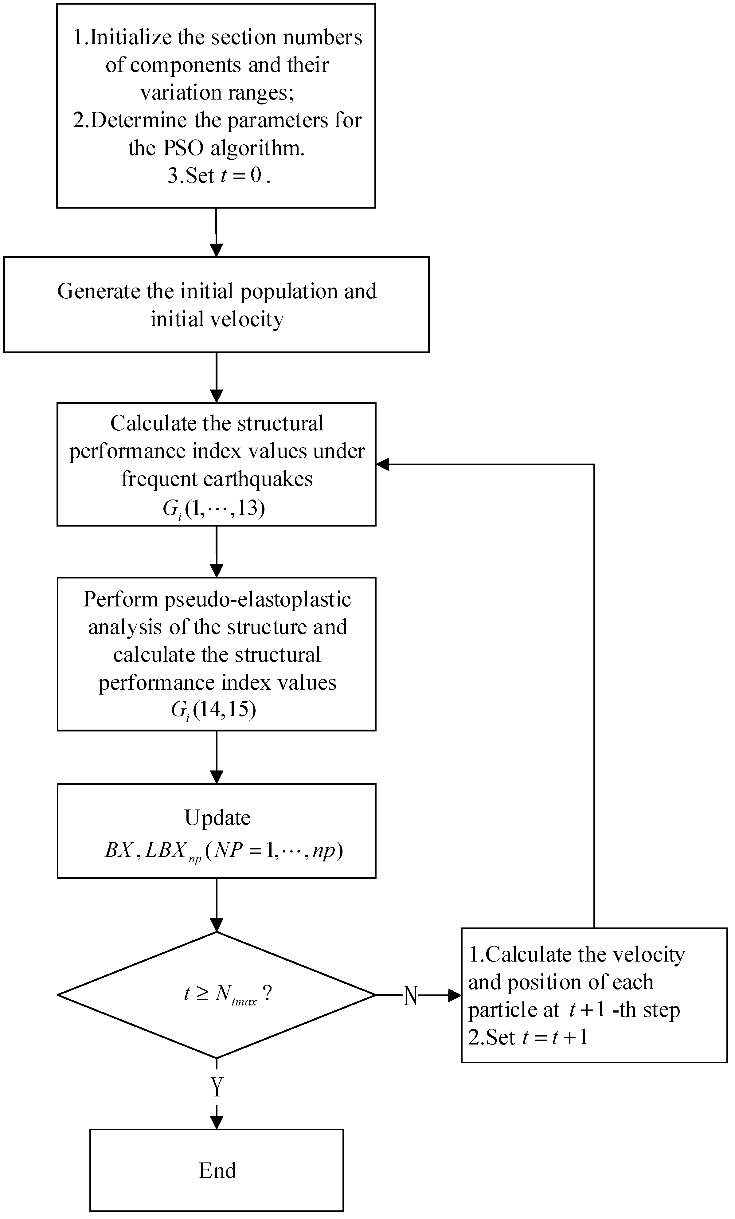
The process for reinforced concrete structure cross-sectional dimension optimization based on the PSO is as follows.

(1) Determine the parameters of the PSO algorithm. Set the number of particles $NP$ to 20, the maximum number of iterations $N_{tmax}$ to 20, the maximum and minimum inertia weights ${\omega }_{\max }$ and ${\omega }_{\min }$ to 0.5, the individual and group learning factors $c_1$ and $c_2$ to 1.3, and the maximum velocity ${\delta }_{\max }$ to 0.5. Obtain the number of variables $NS$, and set the iteration counter $t=0$.

(2) Randomly generate the initial population $X_{np}^0(np=1,2,\cdots ,NP)$ and initial velocity ${\delta }_{np}^0(np=1,2,\cdots ,NP)$.

(3) Based on $X_{np}^t(np=1,2,\cdots ,NP)$, derive $NP$ structural dimension design schemes. For the $np$-th particle, the conversion between its position information $X_{np}^t$ and the component size number vector $S_{np}^t=(s_{np,1}^t,s_{np,2}^t,\cdots ,s_{np,N}^t)$ is defined by Equation (21), where round( ) represents the rounding operation.

$$s_{np,ns}^t=round\left(l_{ns}+X_{np,ns}^t·(u_{ns}-l_{ns})\right)(ns=1,\cdots ,NS)$$

(21)

Use $S_{np}^t(np=1,2,\cdots ,NP)$ to modify the model, perform response spectrum analysis under frequent earthquakes, and quasi-elastic–plastic analysis under rare earthquakes. Calculate the constraint value $G_j\left(X\right)(j=1, 2, \cdots , 15)$ for each particle, and determine the current fitness function of each particle based on Equations (17) and (18).

(4) Update the global historical best position $BX$ and the individual historical best position $LB{X}_{np}$. Calculate the velocity of each particle in iteration step $t+1$, and update the position $X_{np}^{t+1}(np=1,2,\cdots ,NP)$ of each particle.

(5) If $t\ge N_{tmax}$, it indicates that the algorithm has completed all optimization processes, and the current $BX$ is the final optimization solution; otherwise, continue with the next step starting from step (3), and set $t=t+1$. Extensive case studies conducted by the research team indicate that for general building structures, the number of iterations can be set to 20.

The quasi-elastic–plastic optimization flowchart for reinforced concrete structures is shown in Figure 6.

4. Case Study

This article uses two real building models and designs a series of experiments to achieve the following objectives: 1. Perform an analysis and calculation of Model-1 and Model-2 using the quasi-elastic–plastic analysis method. By comparing with the nonlinear time–history analysis method, the accuracy and efficiency of the method proposed in this article are verified. 2. Combine the elastic response spectrum method and the quasi-elastic–plastic analysis method to calculate the performance indicators of the structure in both the elastic and elastic–plastic stages. Then, use the PSO method to optimize the cross-sectional dimensions of the reinforced concrete structure, verifying the effectiveness of the method in the integrated elastic and elastic–plastic optimization. The material prices involved in the example analysis are based on current market prices, as shown in

Table 3. Material price list.

Material Name	Unit Price (Concrete in CNY/m3, Steel in CNY/ton)
C35	570
C40	590
HRB335	5000

. According to the studies indicated in reference [32], for the reinforced concrete frames and frame–shear wall structures in this research, the Kowalsky [33] formula yields relatively small errors when calculating the damping ratio. Hence, the formula is employed to calculate structural damping.

4.1. Model-1 Analysis and Optimization

Model-1 is a 15-story reinforced concrete frame structure, with a first-floor height of 4.2 m and a floor height of 3.6 m for the remaining floors. The total height of the building is 54.6 m, and the plan dimensions are 24 m × 18 m. The concrete strength grade of the main lateral force-resisting components is C40 for floors 1 to 5 and C35 for floors 6 to 15. The elastic moduli of C35 and C40 concrete are 3.15 × 10⁴ N/mm² and 3.25 × 10⁴ N/mm², respectively. The 3D and plan views of the building structure are shown in Figure 7. The design earthquake group is Group 1, the site category is Class II, the shear wave velocity of the soil layers is in the range of 500 m/s to 800 m/s, and the characteristic period is 0.35 s. The main load information is shown in

Table 4. Main load information of Model-1.

Plate Dead Load	Plate Live Load	Beam Dead Load	Seismic Intensity (Acceleration)
4.5 kN/m2	2 kN/m2	4.5 kN/m2	7 (0.15 g)

.

The ductility factor of the structure is 3.35 in the X-direction, and 3.56 in the Y-direction. Based on the Kowalsky damping ratio calculation formula, the equivalent damping ratio is 0.194 in the X-direction, and is 0.200 in the Y-direction. To verify the accuracy of this method, seven natural seismic waves were selected and compared with the results from the dynamic nonlinear time–history analysis. The parameters of the seismic waves are shown in

Table 5. Seismic waves selected for Model-1.

No.	Name	Peak Acceleration in the Primary Direction (cm/s2)	Peak Acceleration in the Sub-Direction (cm/s2)	Duration(s)
1	Chi-Chi, Taiwan-02_NO_1205	638.8	301.9	68.0
2	Coalinga-01_NO_352	121.9	136.8	40.0
3	Gilroy_NO_2039	14.1	23.9	46.0
4	Irpinia, Italy-01_NO_291	103.6	105.9	37.2
5	Morgan Hill_NO_471	69.7	81.0	28.3
6	Northridge-01_NO_1679	11.4	12.0	40.0
7	Yorba Linda_NO_2051	9.4	9.5	36.0

, with the peak acceleration set at 7 degrees (0.15 g), and the rare seismic acceleration is 310 cm/s².

Under rare seismic events, almost all structural damage and a significant portion of non-structural damage in buildings are caused by lateral displacements. Therefore, estimating lateral displacements is critically important. The peak ground acceleration was adjusted to 310 cm/s² in the nonlinear time–history analysis. The results of story drift obtained from the nonlinear time–history analysis method (denoted as TH) and the quasi-elastic–plastic analysis method (denoted as PE) are shown in Figure 8.

It can be observed that the proposed equivalent elastic method produces story drifts along the building height that are generally consistent with those obtained from the time–history analysis method. Similarly, the horizontal displacement at the top of the structure calculated by both methods is also in close agreement. Since the most time-consuming part of the calculation process is structural analysis, the computational efficiency of the method is evaluated by the number of structural analyses conducted in ETABS until model convergence. EX and EY represent the calculation conditions under rare seismic events in the X- and Y-directions, respectively. For the EX, three iterations are required, and the maximum story drift occurs on the 7th floor, with a value of 1/263. Similarly, for the EY, three iterations are needed, with the maximum story drift also occurring on the 7th floor, with a value of 1/228. In the time–history analysis, the maximum story drift for the EX also occurs on the 7th floor, with an average value of 1/285, while for the EY case, it occurs on the 7th floor as well, with an average value of 1/216. The differences between the two methods under seismic loads in the X- and Y- directions are 7.7% and 5.3%, respectively, which are considered acceptable.

In addition to calculating lateral displacements, understanding the damage conditions of structural components is crucial for structural design. Taking axis 3 and axis B in the floor plan of Figure 7 as examples, a comparison of the results from the dynamic nonlinear time–history analysis method and the quasi-elastic–plastic analysis method is presented. Figure 9a,c show the stiffness reduction factors obtained using the quasi-elastic–plastic analysis method, while Figure 9b,d illustrate the component damage values derived from the time–history analysis method. The stiffness reduction factors obtained from the quasi-elastic–plastic analysis method are consistent with the damage conditions calculated by the time–history analysis method, demonstrating the validity of this approach.

Among them, the damage value of a component is obtained by weighting the tensile or compressive damage factors of each fiber, and the weighting coefficient is determined by the product of the fiber area, the strength of the fiber material, and the square of the distance from the fiber to the centroid of the cross-section. The damage value, ranging from 0 to 1, indicates the extent of damage in the component from its state of not yielding to its stress limit.

The quasi-elastic–plastic analysis method provides accurate structural responses. Therefore, using the optimization process outlined in Section 3.3, component section dimensions were optimized to reduce structural costs. Model-1 consists of four standard floors: floor 1, floors 2–5, floors 6–10, and floors 11–15. The corresponding loading conditions for calculating different structural performance indicators during the optimization process are provided in reference [31]. The changes in component dimensions for Model-1 before and after optimization are shown in

Table 6. Changes in component dimensions of Model-1 before and after optimization.

Component Type	Standard Floor	Material Strength Grade	Section Dimensions Before Optimization (mm)	Section Dimensions After Optimization (mm)
Beam	1	C40	700 × 400	650 × 350
	2		700 × 400	650 × 350
	3	C35	700 × 300	650 × 250
	4		700 × 300	650 × 250
Column	1	C40	1000 × 1000	850 × 850
			800 × 800	600 × 600
	2		800 × 800	600 × 600
	3	C35	700 × 700	500 × 500
	4		600 × 600	400 × 400

.

The optimization process considered the structural performance constraints under frequent earthquake conditions and used the quasi-elastic–plastic analysis method to calculate the elastoplastic story drift under rare earthquake conditions. The structural performance indicators under frequent and rare earthquake conditions, as well as the changes in the structural cost, are shown in Figure 10. In Figure 10, iteration 0 corresponds to the initial state, and iteration 1 corresponds to the initial population.

The optimization process iterated 21 times in total, reducing the structural cost from approximately 1.39 × 10⁶ CNY to about 1.15 × 10⁶ CNY. During the optimization, the reinforcement ratio of the components was determined by ETABS according to relevant codes based on component internal forces, and all reinforcement ratios remained within code-specified limits. Throughout the optimization process, constraints $G_1$ and $G_2$, representing the story drifts under frequent earthquake conditions in the X- and Y-directions, showed significant changes and generally increased. The maximum story drift in the Y-direction reached 9/5000 during the 17th iteration, which was very close to the limit of 1/550, and remained at this value until the end of the optimization. At the end of the optimization, all constraints, including the elastoplastic story drift, were within their respective limits. The structure met the performance requirements under both frequent and rare earthquake conditions, demonstrating the effectiveness of the proposed method in the integrated optimization of elastic and elastoplastic performance for reinforced concrete frame structures.

4.2. Model-2 Analysis and Optimization

Model-2 is a 15-story reinforced concrete frame-shear wall structure, with a floor height of 3.6 m and a total height of 49.5 m. The concrete strength grade of the main lateral load-resisting components is C40 for floors 1 to 5, and C35 for floors 6 to 15. The 3D and plan views of the building structure are shown in Figure 11. The main load information is provided in

Table 7. Main load information of Model-2.

Plate Dead Load	Plate Live Load	Beam Dead Load	Seismic Intensity (Acceleration)
4.5 kN/m2	2 kN/m2	4.5 kN/m2	8 (0.2 g)

. The design seismic group is Group 2, with a site category of Class II and a characteristic period of 0.4 s.

The structure ductility coefficient in the X-direction is 3.19, and 3.64 in the Y-direction. The calculated damping ratios in the X- and Y-directions are 0.190 and 0.202, respectively. Seven natural earthquake waves were selected for dynamic nonlinear time–history analysis, and the results were compared with those obtained from the quasi-elastic–plastic analysis method. The peak acceleration was set to 400 cm/s² for rare earthquake conditions. The peak acceleration and duration for each wave are shown in

Table 8. Seismic waves selected for Model-2.

No.	Name	Peak Acceleration in the Primary Direction (cm/s2)	Peak Acceleration in the Sub-Direction (cm/s2)	Duration (s)
1	Borah Peak, ID-01_NO_439	39.7	52.3	39.7
2	Chi-Chi, Taiwan-02_NO-2165	24.0	23.1	55.0
3	Imperial Valley-06_NO_159	370.3	220.9	28.4
4	Kocaeli, Turkey_NO_1172	34.9	36.3	41.4
5	Morgan Hill_NO_461	156.3	311.7	38.0
6	San Fernando_NO_52	27.1	37.1	42.4
7	Whittier Narrows-01_NO_609	34.6	30.6	39.0

.

Figure 12 shows the displacement results calculated using the elastoplastic time–history method and the quasi-elastic–plastic analysis method. Under the EX condition, the maximum story drift calculated by the quasi-elastic–plastic analysis method and the time–history analysis method are both approximately 1/110, with only a 0.7% error. Under the EY condition, the maximum story drift calculated by the quasi-elastic–plastic analysis method is 1/198, while it is 1/192 when calculated by the time–history analysis method, with a 3.4% error. The results from both methods are generally consistent. For lateral displacement of the structure, the floor displacements calculated by both methods are essentially the same. During the analysis, under both the EX and EY conditions, convergence was achieved after performing only six structural analyses in ETABS.

Taking axis 3 and axis A in the floor plan of Figure 11 as examples, a comparison is made between the dynamic nonlinear time–history analysis method and the quasi-elastic–plastic analysis method. Figure 13a,c show the stiffness reduction factors calculated using the equivalent method, while Figure 13b,d show the component damage value calculated by the time–history analysis method. The stiffness reduction factors obtained from the quasi-elastic–plastic analysis method are generally consistent with the damage values calculated by the time–history analysis method.

Model-2 consists of three standard floors, namely floors 1–5, 6–10, and 11–15. The changes in the dimensions of the components in the model before and after optimization are shown in

Table 9. Changes in component dimensions of Model-2 before and after optimization.

Component Type	Standard Floor	Material Strength Grade	Section Dimensions Before Optimization (mm)	Section Dimensions After Optimization (mm)
Beam	1	C40	850 × 550	500 × 350
			900 × 600	750 × 400
	2	C35	800 × 500	500 × 200
			850 × 550	550 × 400
	3		750 × 450	700 × 350
			800 × 500	750 × 400
Column	1	C40	1200 × 1200	1200 × 1200
	2	C35	1100 × 1100	1000 × 1000
	3		1000 × 1000	750 × 750
Wall	1	C40	400	350
	2	C35	380	350
	3		360	350

. The steel reinforcement ratio is determined by ETABS according to relevant design specifications.

The optimization process for structural performance indices and cost under frequent and rare earthquakes is shown in Figure 14. The optimization was iterated 21 times in total, reducing the structural cost from approximately 2.6 × 10⁶ CNY to about 2.4 × 10⁶ CNY. The initial structure of Model-2 was infeasible, with maximum story drifts of 1/602 and 1/782 in the X- and Y-directions under frequent earthquakes, both exceeding the limit of 1/800. Consequently, $G_1$ and $G_2$ were greater than 0. A feasible solution was found in the first iteration, with all constraint values meeting their limits. This resulted in a significant increase in overall component dimensions, raising the cost to approximately 3.6 × 10⁶ CNY. Subsequently, the algorithm continuously adjusted the structural dimensions to achieve a more cost-effective design. During this process, the maximum story drift in the elastic state showed an overall upward trend. The elastoplastic story drifts in the X- and Y-directions, respectively, reached 3/2500 and 1/1000 at the 12th iteration and remained stable until the optimization concluded.

At the end of the optimization, all performance indices for the structure in both elastic and elastoplastic design stages were within the specified limits, and the results met the requirements of the design code. From the optimization results of Model-1 and -2, it can be observed that most structural performance indices in the optimized results still maintain a certain margin from the specified limits. This is attributed to the reason that, due to structural layout constraints, some performance indices may be difficult to approach the specified limits. The optimization method in this study allows the adjustment of structural dimensions to meet constraints, even when the initial structure does not satisfy them. Elastic–plastic structural optimization often requires multiple iterations, and using time–history analysis would incur significant time costs. In contrast, the quasi-elastic–plastic analysis method can efficiently perform elastic–plastic analysis of structures, making it practically meaningful.

5. Conclusions

This article conducts a quasi-elastic–plastic optimization study on reinforced concrete frame–shear wall structures. The proposed quasi-elastic–plastic analysis method transforms the time-consuming nonlinear time–history analysis, which generally results in significant variability, into an elastic analysis of an equivalent model. Combined with optimization theory, this approach significantly reduces the difficulty of elastoplastic optimization for reinforced concrete structures. The specific conclusions are as follows.

(1) A total of 64 shear wall samples were constructed, and their yield bending moments were calculated using XTRACT under varying axial forces, section heights, vertical reinforcement ratios, and tensile reinforcement areas of edge components. An approximate formula for calculating the yield bending moment of shear walls was fitted based on these results. Through computational analysis, it was found that the average error between the yield bending moments calculated using the proposed formula and those obtained from XTRACT was 9% for the selected samples.

(2) Taking a 15-story reinforced concrete frame structure and a 15-story reinforced concrete frame–shear wall structure as examples, the quasi-elastic–plastic analysis method was used to perform calculations on both models, and the results were compared with those from the time–history analysis method. The case studies demonstrated that the quasi-elastic–plastic analysis method can achieve efficient and accurate calculations for both frame structures and frame–shear wall structures.

(3) By combining the quasi-elastic–plastic analysis method with the elastic response spectrum method, the optimization of frame structures and frame–shear wall structures were achieved by adjusting the cross-sectional dimensions of structural components. The optimization process revealed that the structural size optimization of actual buildings often requires hundreds of structural design analyses. Therefore, the proposed quasi-elastic–plastic analysis method can significantly enhance the efficiency of elastic and elastoplastic optimization for reinforced concrete structures, demonstrating strong practical value. Coupled with the particle swarm optimization method, elastic–plastic optimization that meets the requirements of the code can be achieved, and the optimization results can meet 15 structural performance criteria under frequent and rare earthquake conditions, ensuring reliability.

(4) The damping ratios of different structures vary under different plastic states, which introduces limitations to the fixed damping ratio approach used in this article. Furthermore, this study focuses solely on the quasi-elastic–plastic optimization of reinforced concrete structures, without addressing other types of structures. Therefore, future work will aim to extend the quasi-elastic–plastic analysis method to make it applicable to a broader range of scenarios.

References

1. Krawinkler, H.; Seneviratna, G.D.P.K. Pros and cons of a pushover analysis of seismic performance evaluation. Eng. Struct. 1998, 20, 452–464. [Google Scholar] [CrossRef]
2. Kaats𝚤z, K.; Sucuoğlu, H. Generalized force vectors for multi-mode pushover analysis of torsionally coupled systems. Earthq. Eng. Struct. Dyn. 2014, 43, 2015–2033. [Google Scholar] [CrossRef]
3. Daei, A.; Zarrin, M. A multi-mode displacement-based pushover (MDP) procedure for seismic assessment of buildings. Soil Dyn. Earthq. Eng. 2021, 150, 106950. [Google Scholar] [CrossRef]
4. Chopra, A.K.; Goel, R.K.; Chintanapakdee, C. Evaluation of a modified MPA procedure assuming higher modes as elastic to estimate seismic demands. Earthq. Spectra 2004, 20, 757–778. [Google Scholar] [CrossRef]
5. Poursha, M.; Khoshnoudian, F.; Moghadam, A.S. A consecutive modal pushover procedure for estimating the seismic demands of tall buildings. Eng. Struct. 2009, 31, 591–599. [Google Scholar] [CrossRef]
6. Poursha, M.; Khoshnoudian, F.; Moghadam, A.S. The extended consecutive modal pushover procedure for estimating the seismic demands of two-way unsymmetric-plan tall buildings under influence of two horizontal components of ground motions. Soil Dyn. Earthq. Eng. 2014, 63, 162–173. [Google Scholar] [CrossRef]
7. Bracci, J.M.; Kunnath, S.K.; Reinhorn, A.M. Seismic performance and retrofit evaluation of reinforced concrete structures. J. Struct. Eng. 1997, 123, 3–10. [Google Scholar] [CrossRef]
8. Antoniou, S.; Pinho, R. Development and verification of a displacement-based adaptive pushover procedure. J. Earthq. Eng. 2004, 8, 643–661. [Google Scholar] [CrossRef]
9. Kalkan, E.; Kunnath, S.K. Adaptive modal combination procedure for nonlinear static analysis of building structures. J. Struct. Eng. 2006, 132, 1721–1731. [Google Scholar] [CrossRef]
10. Bai, J.; Ou, J. Optimization of failure modes for reinforced concrete buildings based on ida method. Eng. Mech. 2011, 28, 198–203. [Google Scholar]
11. Tang, Y. Intelligent Optimization and Seismic Vulnerability Evaluation of Large-Span Spatial Structures. Master’s Thesis, Chongqing University, Chongqing, China, 2023. [Google Scholar]
12. Liu, P. Research on Mechanical Properties Andseismic Failure Mode for High-Riseprimary-Secondary Structural System. Ph.D. Thesis, Harbin Institute of Technology, Harbin, China, 2019. [Google Scholar]
13. Gülkan, P.; Sozen, M. Inelastic responses of reinforced concrete structures to earthquake motions. J. Am. Concr. Inst. 1974, 71, 604–610. [Google Scholar] [CrossRef]
14. Shibata, A.; Sozen, M.A. The Substitute-Structure Method for Earthquake-Resistant Design of Reinforced Concrete Frames; University of Illinois Engineering Experiment Station: Champaign, IL, USA, 1974. [Google Scholar]
15. Shibata, A.; Sozen, M.A. Substitute-structure method for seismic design in R/C. J. Struct. Div. 1976, 102, 1–18. [Google Scholar] [CrossRef]
16. Yoshida, S.S. Modified Substitute Structure Method for Analysis of Existing R/C Structures. Master’s Thesis, University of British Columbia, Vancouver, BC, Canada, 1979. [Google Scholar]
17. Lin, Y.; Miranda, E. Noniterative equivalent linear method for evaluation of existing structures. J. Struct. Eng. 2008, 134, 1685–1695. [Google Scholar] [CrossRef]
18. Miranda, E.; Lin, Y. Non-iterative equivalent linear method for displacement-based design. In Proceedings of the 13th World Conference on Earthquake Engineering, Vancouver, BC, Canada, 1–6 August 2004. [Google Scholar]
19. Wang, S.; Hua, L.; Yang, C.; Han, X.; Su, Z. Applications of incremental harmonic balance method combined with equivalent piecewise linearization on vibrations of nonlinear stiffness systems. J. Sound Vib. 2019, 441, 111–125. [Google Scholar] [CrossRef]
20. Guyader, A.C.; Iwan, W.D. Determining equivalent linear parameters for use in a capacity spectrum method of analysis. J. Struct. Eng. 2006, 132, 59–67. [Google Scholar] [CrossRef]
21. Samimifar, M.; Massumi, A.; Moghadam, A.S. Proposal of an equivalent linearization method to predict seismic hysteretic energy demand considering stiffness degradation effects. Struct. Des. Tall Spec. Build. 2020, 29, e1740. [Google Scholar] [CrossRef]
22. Wang, D.; Tan, D.; Liu, L. Particle swarm optimization algorithm: An overview. Soft Comput. 2018, 22, 387–408. [Google Scholar] [CrossRef]
23. MOHURD. GB50010-2010; Design Code for Concrete Structures. China Architecture & Building Press: Beijing, China, 2010.
24. Mangalathu, S.; Jang, H.; Hwang, S.-H.; Jeon, J.-S. Data-driven machine-learning-based seismic failure mode identification of reinforced concrete shear walls. Eng. Struct. 2020, 208, 110331. [Google Scholar] [CrossRef]
25. Ji, J.; Xiao, Q.; Huang, C.; Han, X.; Li, S. Research on deformation limits of performance-based RC shear walls controlled by flexure. J. Build. Struct. 2010, 31, 35–41. [Google Scholar] [CrossRef]
26. Ji, X.; Xu, M.; Cheng, X.; Miao, Z. Experimental study on axial tension-flexure-shear behavior of moderate-aspect-ratio RC shear walls. J. Builading Struct. 2021, 42, 90–101. [Google Scholar] [CrossRef]
27. MOHURD. JGJ 3-2010; Technical Specification for Concrete Structures of Tall Buildings. China Architecture & Building Press: Beijing, China, 2010.
28. Ji, X.; Cheng, X.; Xu, M. Experimental study on tension-shear behavior of low-aspect-ratio RC walls. Eng. Mech. 2018, 35, 53–61. [Google Scholar] [CrossRef]
29. Veletsos, A.S.; Newmark, N.M. Effect of inelastic behaviour on the response of simple systems to earthquake motions. In Proceedings of the 2nd World Conference on Earthquake Engineering, Tokyo, Japan, 11–18 July 1960; pp. 895–912. [Google Scholar]
30. Jin, F.; Yang, Y.; Hu, B.; Zhou, J.; Gao, B.; Wan, Y. Research on section dimension optimization of high-rise steel–concrete composite buildings based on improved dividing rectangle algorithm and combined response surface model. Structures 2023, 58, 105437. [Google Scholar] [CrossRef]
31. Lou, H.P.; Ye, J.; Jin, F.L.; Gao, B.Q.; Wan, Y.Y.; Quan, G. A practical shear wall layout optimization framework for the design of high-rise buildings. Structures 2021, 34, 3172–3195. [Google Scholar] [CrossRef]
32. Ma, Y.; Liu, W.; Li, Y. Study of equivalent linearization methods for inelastic analysis of structures. Sichuan Build. Sci. 2008, 34, 153–157. [Google Scholar]
33. Kowalsky, M.J. Displacement-Based Design—A Methodology for Seismic Design Applied to RC Bridge Columns. Master’s Thesis, University of California at San Diego, La Jolla, CA, USA, 1994. [Google Scholar]
Figure 1. Section yield condition diagram. (a) Shear wall cross-section; (b) section stress and strain; (c) concrete stress distribution ( F c denotes the stress resultant); (d) reinforcement stress distribution ( F s , F s w , F s and F s w denote the stress resultant).
Buildings 15 00982 g001
Figure 2. Comparison of yield moment for sample points.
Buildings 15 00982 g002
Figure 3. The ideal elastoplastic member M - Φ curve.
Buildings 15 00982 g003
Figure 4. Energy equivalence diagram.
Buildings 15 00982 g004
Figure 5. Flowchart of quasi-elastic–plastic analysis method for reinforced concrete structures.
Buildings 15 00982 g005
Figure 6. Flowchart of quasi-elastic–plastic optimization for reinforced concrete structures.
Buildings 15 00982 g006
Figure 7. Three-dimensional and plan views of Model-1: (a) 3D view of the building; (b) plan view of 1st floor (size unit: mm); (c) plan view of 2nd to 15th floors (size unit: mm).
Buildings 15 00982 g007
Figure 8. Comparison of results between pseudo-elastoplastic analysis and time–history analysis for Model-1. (a) Story drift; (b) displacement.
Buildings 15 00982 g008
Figure 9. Damage location diagram for Model-1 (stiffness reduction factor for unmarked components is 1). (a) Stiffness reduction factor for axis 3; (b) component damage values for axis 3 in time–history analysis; (c) stiffness reduction factor for axis B; (d) component damage values for axis B in time–history analysis.
Buildings 15 00982 g009
Figure 10. Change in data to iterations of Model-1. (a) Constraint ( G 1 G 8 ); (b) constraint ( G 9 G 15 ); (c) structural cost.
Buildings 15 00982 g010
Figure 11. Three-dimensional and plan views of Model-2: (a) 3D view of the building; (b) plan view of 2nd to 15th floors (Size unit: mm).
Buildings 15 00982 g011
Figure 12. Comparison of results between quasi-elastic–plastic analysis and time–history analysis for Model-2. (a) Story drift; (b) displacement.
Buildings 15 00982 g012
Figure 13. Damage location diagram for Model-2 (stiffness reduction factor for unmarked components is 1). (a) Stiffness reduction factor for axis 3; (b) component damage values for axis 3 in time–history analysis; (c) stiffness reduction factor for axis A; (d) component damage conditions for axis A in time–history analysis.
Buildings 15 00982 g013
Figure 14. Change in data to iterations of Model-2. (a) Constraint ( G 1 G 8 ); (b) constraint ( G 9 G 15 ); (c) structural cost.
Buildings 15 00982 g014