Abstract
Traditional methods of determining structural dynamic parameters produce destructive and unreliable results. Therefore, in this study, operational modal analysis method, which is a non-destructive and advanced method, was used to determine structural dynamic parameters. In this study, the dynamic parameters of the steel garage model were determined by the operational modal analysis (OMA), method and the current status of the structure was evaluated. The finite element model (FEM) of the steel garage was created with SAP2000 software, and then the experimental data were analyzed with Artemis Modal Pro software. When the FEM and OMA results were compared, it was seen that the frequency values obtained for the first five modes were quite close. When the damping ratios were examined, significant differences were detected between the theoretical and experimental values in some modes. It was determined that using the experimental damping ratios instead of the constant damping ratio assumed in the FEM would give more accurate results. Provided that the modeling and measurement stages are carried out meticulously, the operational modal analysis method as a non-destructive testing method is recommended to be used to obtain dynamic parameters in structures similar to the steel garage model.
1. Introduction
There are many methods to evaluate the dynamic performance of structures. However, many old methods (coring, etc.) damage the existing structure. They also do not fully represent the structure. Especially in reinforced concrete structures, the process ends with both damage to the structure and failure to obtain a reliable result because it is impossible for the material properties to be homogeneous depending on the application. When other uncalculated external environmental conditions are added to this, it is concluded that the result is not very reliable, and destructive structure parameter determination methods remain primitive. For this reason, non-destructive structure property determination methods have been developed in recent years, and many experimental studies have been conducted in many different countries of the world in this field [1,2,3,4,5,6,7].
Operational modal analysis (OMA) is an important technique used in the process of experimental investigation and the modeling of structural dynamics. It has great importance in determining the vibration modes and frequencies of structures, especially in engineering fields. OMA is an approach to the description of dynamic systems, usually supported by measurement techniques such as structural monitoring, vibration testing, and the frequency response function. In recent years, this analysis technique has been developed to overcome the limitations of traditional modal analysis methods and has found a much wider application range [8,9]. The study [10] explains the theoretical basis and application areas of the classical modal analysis method in detail, while examining the reasons why the operational modal analysis method is preferred more in practice. Operational modal analysis provides a faster and more cost-effective approach than traditional modal analysis methods by using environmental vibrations to determine the natural frequencies, mode shapes, and damping ratios of structures. The authors state that the operational modal analysis method is extremely useful, especially for examining existing structures and obtaining dynamic parameters. While operational modal analysis involves experimental studies by observing the natural vibrations of the structure, using only the vibrations due to environmental conditions without applying an external stimulus (e.g., a shock or vibration source) makes this technique particularly advantageous [11,12,13]. This feature of OMA offers a much less invasive approach compared to traditional modal analyses, thus allowing it to be easily used in various application areas, especially in industrial structures.
SSI-CVA (Stochastic Subspace Identification–Covariance Variance Analysis) parameter estimation has found a wide application range in recent years as an important method, especially in modeling structural dynamics and system identification. This approach allows for the estimation of model parameters with data obtained from measurements of the natural vibrations and dynamic behaviors of structural systems under environmental noise and random stimuli. The SSI-CVA method was developed to overcome the difficulties encountered by classical time domain and frequency domain-based analysis techniques [14,15,16]. The study [17] discusses the advantages of data-based approaches over traditional modal analysis methods. Stochastic subspace methods allow more accurate results to be obtained with less data and accelerate the process of structural health monitoring. It is also stated that these methods can better handle noise caused by factors such as environmental effects and structural changes. The main advantage of SSI-CVA is that it allows for more accurate and reliable determination of the modal parameters (frequencies, mode shapes, attenuation rates) of complex structural systems. This technique provides accurate results at lower costs, especially in cases where observations of the system are insufficient or direct measurements are not possible [18,19,20,21]. One of the most important features of SSI-CVA is that it minimizes environmental noise and other external effects in the process of estimating unknown parameters of the system by taking advantage of the covariance structure of the data [8]. This makes it much more flexible and practical in terms of application. In recent years, the use of SSI-CVA as an effective tool in structural health monitoring, vibration testing, structural analysis, and maintenance processes has increased [22]. This method has made great contributions to the assessment of the safety and durability of structures in various industrial fields. In the study titled “Analysis of Bridges Using Stochastic Subspace Identification Method with Automatic Modal Analysis Method: Validation with Three Different Bridges” written by Cho and Cho (2023), a stochastic subspace identification (SSI) method is presented to perform automatic modal analysis of bridges. The aim of this research is to verify the effectiveness of the SSI method in determining modal parameters such as natural frequencies, mode shapes, and damping ratios from the vibration data of bridges. The study tests its accuracy and robustness by comparing the results of the SSI method applied to three different bridges. The authors emphasize that modal analysis is very important for evaluating the dynamic behavior of bridges and that these analyses may reveal structural problems that cannot be detected by traditional inspection methods [23]. The study [24] explains the advantages of the SSI method and makes a comparative assessment with traditional modal analysis methods. It is stated that the SSI method provides more accurate results with less data, can quickly determine system parameters, and offers a powerful tool for monitoring complex structures. It is also emphasized that it is effective in detecting changes caused by environmental conditions and structural damage.
Steel garage structures are one of the structural solutions frequently preferred in modern civil engineering due to their durability, cost-effectiveness, and rapid assembly. The advantages of steel materials such as high strength, lightness, and flexibility play an important role in the design and construction of garage structures. Steel garage structures, which offer a wide range of uses, especially in industrial, commercial, and private areas, from vehicle parking to storage, meet important engineering requirements in terms of dynamic loads, environmental factors, and longevity [25,26]. While developments in the design and production stages of steel materials make it possible to provide more efficient and sustainable solutions, the analysis methods used in structural engineering have also become increasingly sophisticated [27]. Dynamic analysis of the structural systems of steel garages is an important area of research, especially for these structures. Advanced simulation and experimental techniques are used to evaluate the seismic performance of structures and to understand the effects of dynamic effects such as environmental loads and user movements on structural integrity [28]. In recent years, improvements in the engineering design of steel garages have allowed structures to be constructed at lower costs and to be assembled more quickly [29,30,31]. The authors of [32] discuss the potential of intelligent monitoring systems for monitoring the dynamic behavior of steel garages. These systems improve structural health monitoring (SHM) processes, allowing for real-time monitoring of the condition of structures and early detection. The study details how sensors and data acquisition methods are integrated to monitor deformations, vibrations, and other dynamic parameters in steel garages and how these data are converted into structural analyses. This study makes a significant contribution to the use of structural health monitoring systems in large and complex structures such as steel garages. It is emphasized that structural health monitoring systems are an effective tool for more accurately monitoring the dynamic behavior of structures, improving maintenance processes, and increasing structural safety. The integration of smart monitoring systems into steel garages has further improved their long-term reliability, allowing for the real-time assessment of structural conditions and predictive maintenance strategies [32,33].
The purpose of this study is to obtain the dynamic parameters of the constructed steel garage model and reveal its current status. Thus, it aimed to reveal any workmanship errors and incompatibilities. In addition, the necessity of reinforcement or reconstruction options for structural health will be evaluated according to the parameters obtained from the steel garage structure. As can be seen in studies in the literature, the structural health monitoring system has generally been used in the measurement and monitoring of previously constructed structures. However, this study also addresses the structural health monitoring system as a structural inspection mechanism, compliance with the project, and the finite element model, as soon as the construction phase is completed. In particular, determining the effect of this situation on the modal parameters by adding cross elements that will disrupt the symmetry of the structure is also addressed. Thus, auto-control of the success of the method is provided in the study.
2. Modal Parameter Extraction with SSI
The stochastic subspace identification technique (SSI) is a time domain method that directly works with raw time data, without the need to convert them into correlations or spectra. The stochastic subspace identification algorithm identifies the state-space matrices based on the measurements by using robust numerical techniques. Once the mathematical description of the structure (the state-space model) is found, it is straightforward to determine the modal parameters. The theoretical background is given in studies by Overschee and De Moor [14], as well as Peeters [21]. The model of vibration structures can be defined by a set of linear, constant coefficient, and second-order differential equations, as shown by Peeters [21]:
where are the mass, damping, and stiffness matrices, is the excitation force, and is the displacement vector at continuous time . is an input influence matrix, characterizing the locations and type of known inputs, . The state-space model originates from control theory, but it also appears in mechanical–civil engineering to compute the modal parameters of a dynamic structure with a general viscous damping model, as shown by Ewins [8]. The equation of motion (1) is transformed to the state-space form of first-order equations, i.e., a continuous-time state-space model of the system is evaluated as
And Equation (4)
where is the state matrix, is the input matrix, and is the state vector. The number of elements of the state-space vector is the number of independent variables needed to describe the state of a system. If it is assumed that the measurements are evaluated at only one sensor location and that these sensors can be accelerometers, velocity, or displacement transducers (accelerometers), the observation equation is
where are the outputs, and are the output matrices for acceleration, velocity, and displacement. With these definitions
Equation (6) can be transformed into
where is the output matrix and is the direct transmission matrix. Equations (2) and (9) constitute a continuous-time deterministic state-space model. Continuous time means that the expressions can be evaluated at each time instant and deterministic means that the input–output quantities can be measured exactly. Of course, this is not realistic: measurements are available at discrete time instants, , with , and the sample time and noise are always influencing the data. After sampling, the state-space model looks like
where is the discrete-time state vector; is the process noise due to disturbance and modeling imperfections; and is the measurement noise due to the sensors’ inaccuracies. The stochastic noise was included, and we obtained the following discrete-time combined deterministic–stochastic state-space model:
are non-measurable vectors, but it is assumed that they are white noise with a zero mean. If this white noise assumption is violated, in other words, if the input also contains some dominant frequency components in addition to white noise, these frequency components cannot be separated from the eigenfrequencies of the system and they will appear as eigenvalues of the system matrix .
where is the expected value operator and is the Kronecker delta. The vibration information that is available in structural health monitoring (SHM) is usually the responses of a structure excited by the operational inputs, which are some immeasurable inputs. Due to the lack of input information, it is not possible to distinguish deterministic the input from the noise terms as described in [34]. If the deterministic input term is modeled by the noise terms the discrete-time purely stochastic state-space model of a vibration structure is obtained:
3. Description of Steel Garage Model
The steel garage model was created as an experimental model. Pictures of the steel garage model are given in Figure 1.
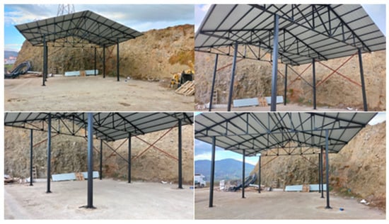
Figure 1.
Pictures of the steel garage model.
Before creating the steel garage model, the ground was leveled and smoothed, and 15 cm thick, ground-leveling, C30 class (TS 500) [35] concrete was poured onto it, as seen in Figure 1. The steel garage structure was fixed to the concrete ground by anchoring it with four M24 anchor bolts from the pole flanges. The poles were connected to the concrete ground with a 10 mm thick and 300 × 300 mm anchor plate. Thus, a 15 cm concrete foundation layer was created under each pole, and the steel garage model was fixed to the ground [36,37]. The steel garage model was created by placing three roof trusses on six poles. The steel garage structure was initially designed symmetrically. In order to disrupt the symmetry, diagonal and x-type central crosses were added to the outer frames. Thus, we aimed to create a self-control mechanism for the operational modal analysis results. It is known that the effect of these additions, especially made in the mod shapes, should be seen. The steel garage structure has a pole opening of 5 m in the X axis direction. The opening of the roof truss in the X axis direction is 8 m. The roof truss is fixed to the poles by welding in the X axis direction with 1.5 m increments on the right and left. The steel garage structure consists of two equal openings in the Y axis direction. The opening width is 3 m each. The pole lengths are 4 m, and the roof truss height is 1.5 m. The poles of the steel garage model are made of a 100 × 100 × 5.4 mm box profile. The lower head, upright, and diagonal elements of the roof truss are made of a 100 × 50 × 4 mm box profile. A 60 × 60 × 3.6 mm box profile is used in purlins and rafters. In addition, a 60 × 60 × 3.6 mm box profile is used in all cross elements between the poles in the steel garage model. A 0.5 mm steel trapezoidal sheet was used in the roof cover. All profiles and sheets used in the steel garage structure were manufactured from S450 steel in accordance with EN-1993-1-1 [37] PER EN 10025-2 [38] standards. The dimensions and element sizes of the steel garage structure are discussed in detail through the finite element model.
4. Finite Element Model of Steel Garage
The finite element model of the steel garage model was created using SAP2000 V26 software [39]. All supports are modeled as fully fixed [36,37]. The members of the steel garage model are modeled as rigidly connected together at the intersection points. While modeling, S450 steel, which was used in the real structure, was used as the material. The elasticity modulus of S450 class steel is 201 Gpa, the unit volume weight is 7.849 t/m3, and the Poisson ratio is 0.3. The roof cover was assigned as mass to the nodes by calculating its mass. In addition, the 50 cm increase in both directions of the roof top cover in the Y axis direction was assigned as mass. A total of 34.176 kg of mass was added to the relevant nodes. The finite element model and element dimensions of the steel garage model are given in Figure 2.
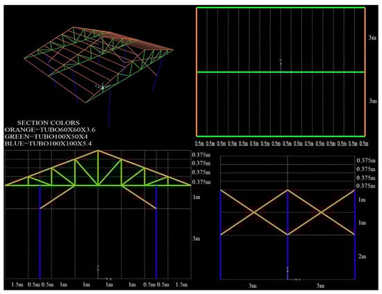
Figure 2.
FE model of the steel garage and dimensions.
The mode shapes of the first five modes of the steel garage model, which were realized with the finite element method, are given in Figure 3, Figure 4, Figure 5, Figure 6 and Figure 7, respectively.
Figure 3.
First-mode shape (f = 2.699 Hz).
Figure 4.
Second-mode shape (f = 3.491 Hz).
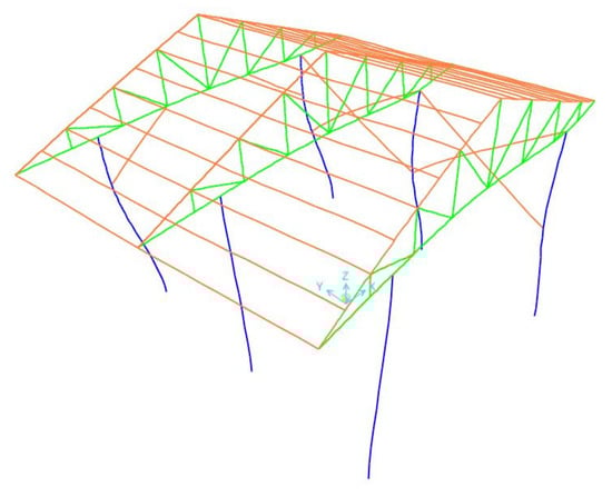
Figure 5.
Third-mode shape (f = 5.223 Hz).
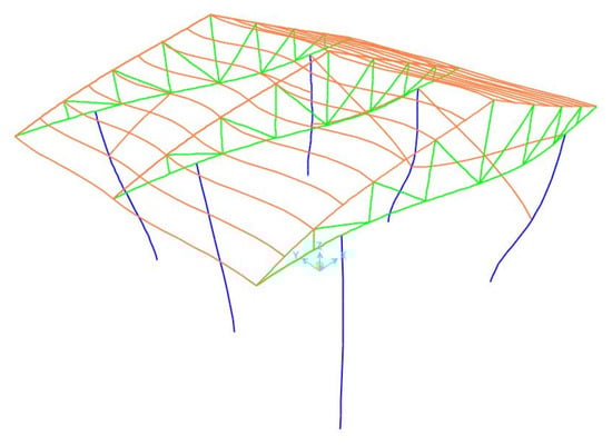
Figure 6.
Fourth-mode shape (f = 8.560 Hz).
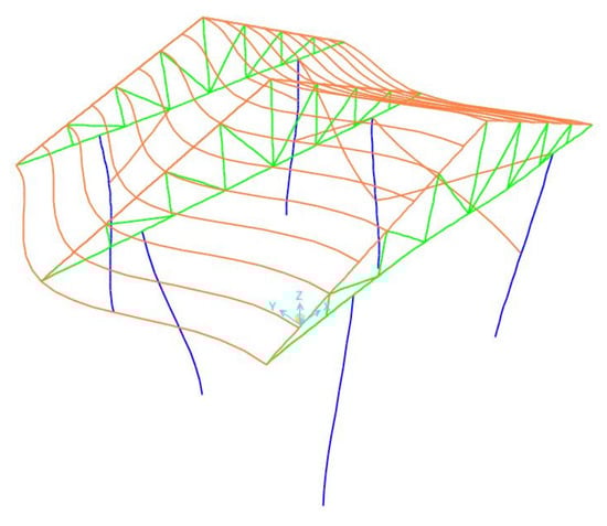
Figure 7.
Fifth-mode shape (f = 9.496 Hz).
The modal analysis results for first five modes of the steel garage model performed with the finite element method are given in Table 1.

Table 1.
The modal analysis results from the finite element analysis (FEA) model.
5. Operational Modal Analysis Model of Steel Garage
Before performing the operational modal analysis, attention was paid to the conformity of the steel garage structure to the project and to the lack of bolts in the connection details. The aim here is to increase the objectivity of the results and the validity of the operational modal analysis. The next step after preparing the steel garage model for operational modal analysis is the calibration of accelerometers and dataloggers. In this study, six three-axis accelerometers and three four-channel dataloggers were used. The technical specifications of the accelerometers used for operational modal analysis are given in Table 2.
Table 2.
The technical specifications of the accelerometers.
The technical specifications of the dataloggers used for operational modal analysis are given in Table 3.
Table 3.
The technical specifications of the data loggers.
The steel garage model prepared for measurement for operational modal analysis is given in Figure 8.
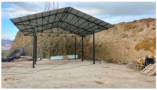
Figure 8.
The steel garage model prepared for measurement for operational modal analysis.
The locations of the accelerometers were determined with FEMtools 3.3 software [40]. Since there were sufficient accelerometers, the reference accelerometer was not used, and the measurement was performed in one go. The accelerometers were fixed to the relevant nodes with hot glue and strong double-sided tape. Testlab Network and MATLAB R2023a software [41] were used for accelerometer calibrations and data conversion with Fast Fourier Transform (FFT). Artemis Modal Pro 4.0 software [42] was used for parameter estimation. The layout plans for the accelerometers are given in Figure 9.
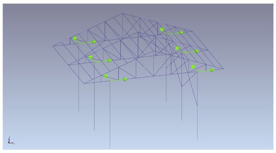
Figure 9.
Accelerometers’ layout.
Measurements were made at approximately 17 degrees Celsius and 63% humidity. Similar measurements were repeated to increase the data set security and for optimum purposes. Data sets that had unwanted noise were canceled. During the measurement, the “start measurement after 10 min” option in the datalogger software was used to adjust the time required to move away from the steel garage structure. In addition, at the time of measurement, peoples were kept approximately 250 m away from the steel garage structure. In this way, the possibility of the accelerometers being affected by white noise was reduced and the measurement data were provided with more reliable results. Among the repeated measurements, consistent data sets were taken as a basis many times. A frequency of 200 Hz was selected as the measurement step based on previous studies. In calculating the measurement period, the “Introduction to Operational Modal Analysis” book [43] was taken into account. The measurement time relation taken from the Introduction to Operational Modal Analysis book is given in Equation (17).
Here, represents the minimum measurement period, and represents the theoretical damping ratio of the structure type. In this study, the damping ratio for steel structures was taken as 0.02. According to Equation (17), the minimum measurement period was found to be 500 s. In order to make the measurements more reliable, the measurement period was taken as 600 s. The data were processed with Artemis Modal Pro 4.0 software [42]. Detrending and filtering processes were performed. Lowpass was selected as the filtering method in the collection and processing of data. The SSI-CVA (Stochastic Subspace Identification–Canonical Variate Analysis) method, which is a time domain method, was used to obtain the parameters. The spectral density matrices are given in Figure 10.
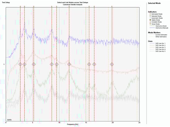
Figure 10.
The spectral density matrices.
The mode shapes of the first five modes of the steel garage model, which were realized with the operational modal analysis, are given in Figure 11, Figure 12, Figure 13, Figure 14 and Figure 15, respectively.
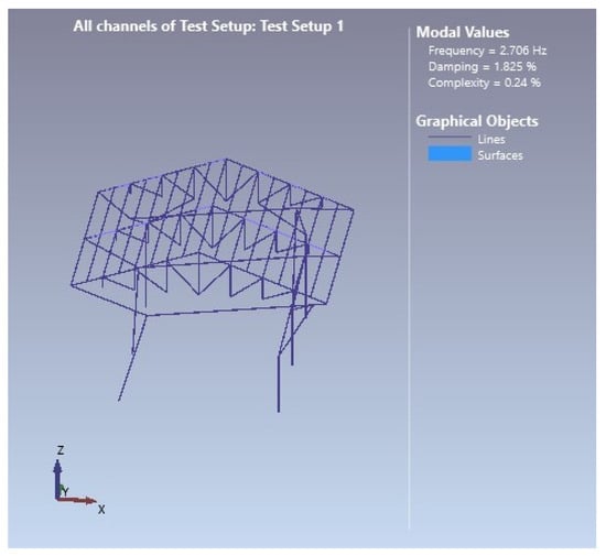
Figure 11.
First-mode shape (f = 2.706 Hz).
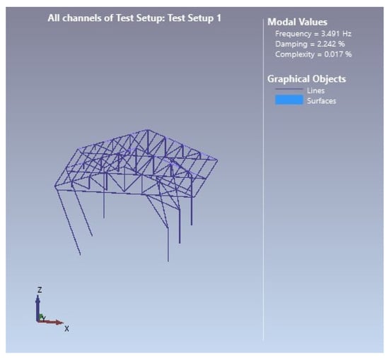
Figure 12.
Second-mode shape (f = 3.491 Hz).
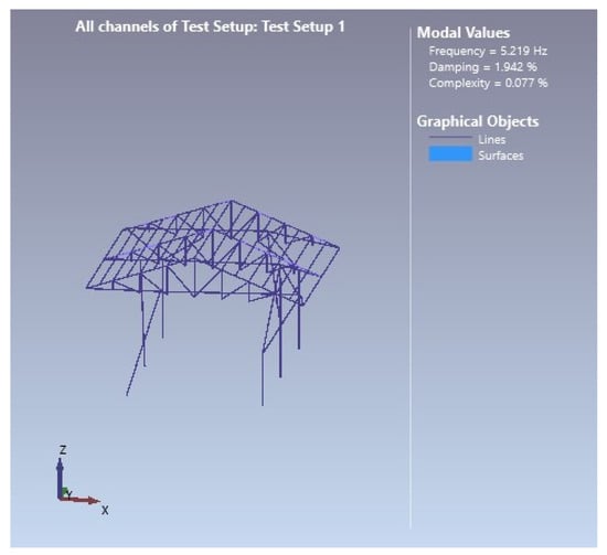
Figure 13.
Third-mode shape (f = 5.219 Hz).
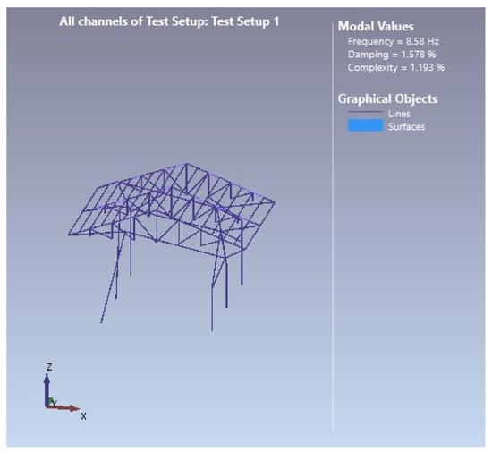
Figure 14.
Fourth-mode shape (f = 8.580 Hz).
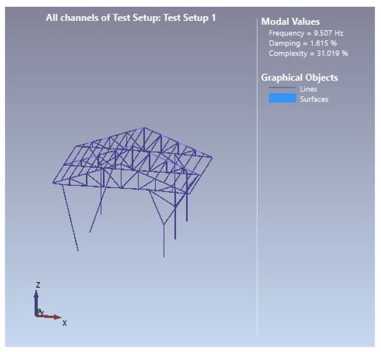
Figure 15.
Fifth-mode shape (f = 9.507 Hz).
The modal analysis results for first five modes of the steel garage model performed with the operational modal analysis are given in Table 4.
Table 4.
The modal analysis results from the operational modal analysis (OMA) model.
In order to determine the validity and reliability of the obtained data, the modal assurance criterion (MAC) should be examined. The aim of the MAC is to show the matching of analytical and experimental mode shapes and the harmony between them, rather than comparing the validity of the obtained experimental data by looking only at the analytical frequency values. The modal assurance criterion (MAC) is a measure of the square cosine of the angle between two modal shapes. The equational expression of the MAC matrix is given in Equation (18).
The FEMtools 3.3 software [40] was used to match the experimental (operational) and finite element mode shapes and to obtain the modal assurance criterion (MAC) matrix. The modal assurance criterion (MAC) diagonal matrix is given in Figure 16.
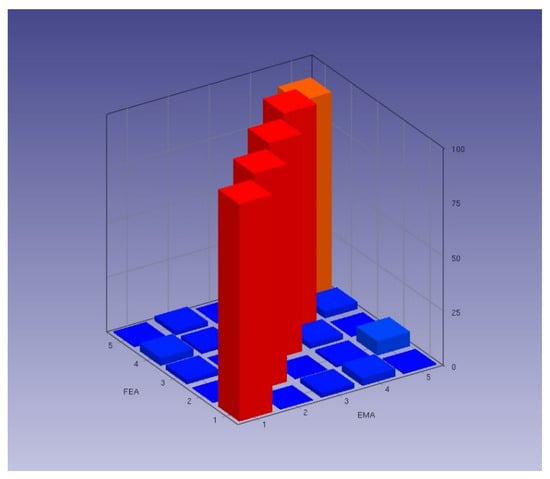
Figure 16.
The modal assurance criterion (MAC) matrix.
The numerical values of the modal assurance criterion (MAC) matrix are given in Equation (19).
The first five modes were paired using FEMtools 3.3 software [40]. The pairing of the experimental (operational) and finite element mode shapes of the first five modes is given in Figure 17, Figure 18, Figure 19, Figure 20 and Figure 21. In Figure 17, Figure 18, Figure 19, Figure 20 and Figure 21, the blue lines represent the FE model and the red lines represent the TEST model.
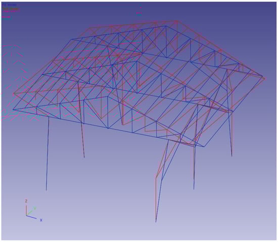
Figure 17.
First-mode shape pairing.
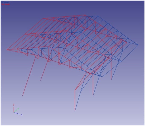
Figure 18.
Second-mode shape pairing.
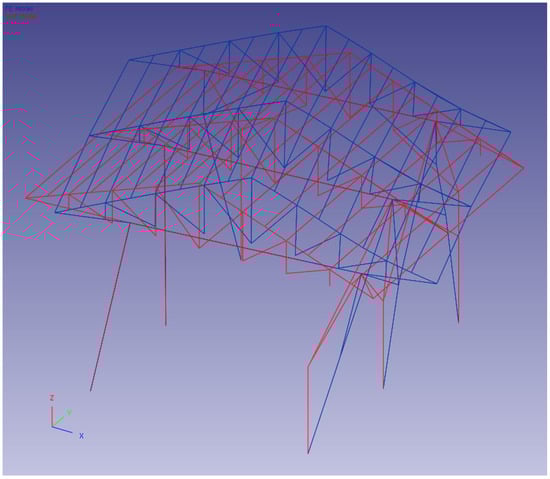
Figure 19.
Third-mode shape pairing.
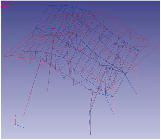
Figure 20.
Fourth-mode shape pairing.
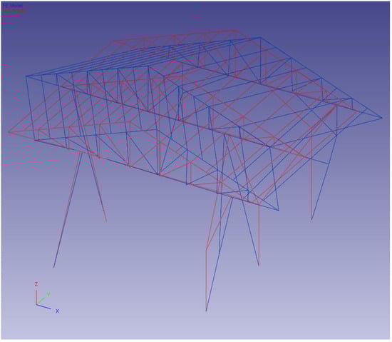
Figure 21.
Fifth-mode shape pairing.
A comparison of the frequency values of the first five modes obtained by the finite element (FE) method and the operational modal analysis (OMA) method is given in Table 5.
Table 5.
Comparison of frequency values (FE-OMA).
The comparison of the mode shape directions of the first 5 modes obtained by the finite element (FE) method and the operational modal analysis (OMA) method is given in Table 6.
Table 6.
Comparison of mode shape directions (FE-OMA).
A comparison of the damping ratio of the first five modes obtained by the finite element (FE) method and the operational modal analysis (OMA) method is given in Table 7.
Table 7.
Comparison of damping ratios (FE-OMA).
When the frequencies of the first five modes obtained with the finite elements of the steel garage model and the frequencies of the first five modes obtained with operational modal analysis were compared, it was seen that the differences were quite small in terms of % and Hz.
When the mode shapes of the first five modes obtained with the finite elements of the steel garage model and the mode shapes of the first five modes obtained with operational modal analysis are compared, it is seen that the differences are quite small. As a result of mode shape matching, only small differences in the eigenvalue vectors in the roof section are noticeable in the modes. However, it is seen that the translation and torsion directions of the mode shapes are similar.
Differences in frequency and mode shapes were determined to have occurred due to the neglection of the mass that is formed by the overlap lengths of the trapezoidal sheets used in the roof cover in the finite element model, the neglection of the bolt and weld mass at the connection points, and the effect of the anti-rust paint applied to the steel profiles during the finite element model update.
In addition, the experimental (real) damping ratios of the steel garage model in the first five modes were obtained. It is an accepted fact that the damping parameter is a very important parameter for the dynamic performance of the structure. With an increase in the damping ratio, the structural system can absorb the acting dynamic forces more. Or, as the damping ratio decreases, the dynamic forces acting on the structural system can increase. In order to determine the real dynamic forces acting on the real structural system, the correct determination of the damping ratio is required. In the finite element model, the theoretical damping ratio is accepted as 2% for steel in all modes [44,45]. However, with the operational modal analysis, the damping ratios for each mode in the first five modes were obtained differently. Especially in the first mode, the experimental damping ratio was obtained as 1.825%. This shows that the system has 0.175% less damping than the accepted damping ratio. In the second mode, the damping ratio was obtained as 2.242%, and this value is 0.242% more than the fixed damping ratio. In the third mode, the damping ratio was obtained as 1.942%, and this value is 0.058% less than the fixed damping ratio. In the fourth mode, the damping ratio was obtained as 1.578%, and this value is 0.422% less than the fixed damping ratio. Among the modes examined, it was determined that the damping ratio was lowest in the fourth mode, and the difference was found to be too large to be neglected. It was understood that these decreases corresponded to approximately one-fifth of the fixed damping ratio. In the fifth mode, the damping ratio was obtained as 1.625%, and this value was 0.385% less than the fixed damping ratio. For all these reasons, it is thought that using experimental damping instead of using fixed damping in dynamic analyses will help to achieve more accurate parameter estimation and will also represent the system more accurately.
6. Conclusions
In light of the results obtained, it was concluded that there was no need to update the support conditions of the steel garage structure, that the support conditions were constructed correctly and in accordance with the finite element model, that the nodal rigidities and therefore the connection elements were constructed in accordance with the finite element model, and that the defined elements were produced in accordance with the defined standards (TS 500 [35] for concrete; EN-1993-1-1 [37] PER EN 10025-2 [38] for steel).
Also, the experimental damping ratios for the first five modes were obtained through operational modal analysis, revealing variations from the fixed damping ratio of 2%. By obtaining experimental damping ratios, the mathematical model of the system was created more reliably, thus enabling realistic results to be obtained in simulating dynamic effects in future.
Provided that the modeling and measurement stages are carried out meticulously, the operational modal analysis method as a non-destructive testing method can be used to obtain dynamic parameters in structures similar to the steel garage model. In addition, it is recommended to use the structural health monitoring method in the compliance inspection of the project and for the compliance control of finite element models, not only in existing steel garage structures but also in newly constructed steel garage structures. In this way, possible construction and production errors can be identified from the very beginning, and early precautions can be taken to prevent damage to the structure, sudden collapse, and loss of life in future use.
Funding
This research received no external funding.
Data Availability Statement
Data are contained within the article; further inquiries can be directed to the author.
Conflicts of Interest
The author declares no conflicts of interest.
References
- Tuhta, S.; Aydin, H.; Günday, F. Updating for Structural Parameter Identification of the Model Steel Bridge Using OMA. Int. J. Latest Technol. Eng. Manag. Appl. Sci. 2020, 9, 59–68. [Google Scholar]
- Tuhta, S.; Günday, F. Application of OMA on The Bench-scale Aluminum Bridge Using Micro Tremor Data. Int. J. Adv. Res. Innov. Ideas Educ. 2019, 5, 912–923. [Google Scholar]
- Kasimzade, A.A.; Tuhta, S.; Günday, F.; Aydın, H. Obtaining Dynamic Parameters by Using Ambient Vibration Recordings on Model of The Steel Arch Bridge. Polytech. Civil. Eng. 2021, 65, 608–618. [Google Scholar] [CrossRef]
- Tuhta, S.; Günday, F. Investigation of Effect of Using Nano Coating on Wooden Sheds on Dynamic Parameters. Wood Res. 2021, 66, 1006–1014. [Google Scholar] [CrossRef]
- Kasimzade, A.A.; Tuhta, S.; Günday, F.; Aydın, H. Investigation of Modal Parameters on Steel Structure Using FDD from Ambient Vibration. In Proceedings of the 8th International Steel Structures Symposium, Konya, Turkey, 24–26 October 2019. [Google Scholar]
- Kasimzade, A.A.; Tuhta, S.; Günday, F.; Aydın, H. Determination of Modal Parameters on Steel Model Bridge Using Operational Modal Analysis. In Proceedings of the 8th International Steel Structures Symposium, Konya, Turkey, 24–26 October 2019. [Google Scholar]
- Tuhta, S.; Günday, F. Determination of The Effect of TiO2 on The Dynamic Behavior of Scaled Concrete Chimney by Oma. MatTech 2021, 55, 459–466. [Google Scholar] [CrossRef]
- Ewins, D.J. Modal Testing: Theory, Practice and Application; Research Studies Press: London, UK, 2000. [Google Scholar]
- Jacobsen, N.J.; Andersen, P.; Brincker, R. Eliminating the influence of harmonic components in operational modal analysis. In Proceedings of the IMAC-XXIV: A Conference & Exposition on Structural Dynamics, Orlando, FL, USA, 19–22 February 2007; Society for Experimental Mechanics: Norfolk, VA, USA, 2007. [Google Scholar]
- Grosel, J.; Sawicki, W.; Pakos, W. Application of classical and operational modal analysis for examination of engineering structures. Procedia Eng. 2014, 91, 136–141. [Google Scholar] [CrossRef]
- Worden, K.; Manson, G. The application of machine learning to structural health monitoring. Philos. Trans. R. Soc. A Math. Phys. Eng. Sci. 2007, 365, 515–537. [Google Scholar] [CrossRef]
- Au, S.K. Operational Modal Analysis; Springer: Singapore; Liverpool, UK, 2017. [Google Scholar]
- Batel, M. Operational modal analysis-another way of doing modal testing. Sound Vib. 2002, 36, 22–27. [Google Scholar]
- Van Overschee, P.; De Moor, B.L. Subspace Identification for Linear Systems: Theory-Implementation Applications; Springer Science-Business Media: New York, NY, USA, 1996. [Google Scholar]
- Berthold, J.; Kolouch, M.; Wittstock, V.; Putz, M. Identification of modal parameters of machine tools during cutting by operational modal analysis. Procedia CIRP 2018, 77, 473–476. [Google Scholar] [CrossRef]
- Zhang, G.; Tang, B.; Tang, G. An improved stochastic subspace identification for operational modal analysis. Measurement 2012, 45, 1246–1256. [Google Scholar] [CrossRef]
- Shokravi, H.; Shokravi, H.; Bakhary, N.; Rahimian Koloor, S.S.; Petrů, M. A comparative study of the data-driven stochastic subspace methods for health monitoring of structures: A bridge case study. Appl. Sci. 2020, 10, 3132. [Google Scholar] [CrossRef]
- Peeters, B.; De Roeck, G.; Pollet, T.; Schueremans, L. Stochastic subspace techniques applied to parameter identification of civil engineering structures. In Proceedings of the New Advances in Modal Synthesis of Large Structures: Nonlinear, Damped and Nondeterministic Cases, Lyon, France, 5–6 October 1995; pp. 151–162. [Google Scholar]
- Peeters, B.; De Roeck, G. Reference-based stochastic subspace identification for output-only modal analysis. Mech. Syst. Signal Proc. 1999, 13, 855–878. [Google Scholar] [CrossRef]
- Peeters, B.; De Roeck, G. One-year monitoring of the Z24-bridge: Environmental influences versus damage events. Earthq. Eng. Struct. Dynam 2001, 30, 149–171. [Google Scholar] [CrossRef]
- Peeters, B.; De Roeck, G. Reference based stochastic subspace identification in civil engineering. Inverse Probl. Eng. 2000, 8, 47–74. [Google Scholar] [CrossRef]
- Ubertini, F.; Comanducci, G.; Cavalagli, N.; Pisello, A.L.; Materazzi, A.L.; Cotana, F. Environmental effects on natural frequencies of the San Pietro bell tower in Perugia, Italy, and their removal for structural performance assessment. Mech. Syst. Signal. Process. 2017, 82, 307–322. [Google Scholar] [CrossRef]
- Cho, S.; Cho, H. Automatic modal analysis of bridges using stochastic subspace identification method: Verification through three different bridges. Appl. Sci. 2023, 13, 12274. [Google Scholar] [CrossRef]
- Bakhary, N.; Rahimian Koloor, S.S.; Petrů, M. Health Monitoring of Civil Infrastructures by Subspace System Identification Method: An Overview. Appl. Sci. 2020, 10, 2786. [Google Scholar] [CrossRef]
- Gustafsson, H.; Nilsson, P.; Eriksson, L. Structural Performance of Steel Garages Under Dynamic Loads. J. Struct. Eng. 2014, 140, 215–230. [Google Scholar]
- Lee, S.; Kim, J. Design Optimization of Steel Garage Structures for Enhanced Durability and Cost Efficiency. Eng. Struct. 2018, 165, 123–134. [Google Scholar]
- Baker, M.; Li, R. Advances in Steel Construction: Applications in Garage Design. J. Struct. Mech. 2010, 58, 87–102. [Google Scholar]
- Yalçın, C.; Kaymaz, A. Seismic Analysis of Steel Garage Structures Using FEM Approaches. Earthq. Eng. 2017, 30, 55–69. [Google Scholar]
- Feng, Y.; Zhi, T. Prefabricated Steel Garage Systems: Innovations and Challenges. Constr. Sci. 2015, 72, 178–194. [Google Scholar]
- Wang, H.; Liu, X.; Zhou, P. Modular Steel Structures for Rapid Construction: A Case Study of Garage Buildings. J. Mod. Constr. 2016, 91, 312–328. [Google Scholar]
- Zhang, T.; Zhao, B.; Chen, L. Corrosion Resistance of Steel Garage Structures in Harsh Environments. Mater. Sci. Eng. 2019, 47, 99–112. [Google Scholar]
- Kwon, Y.; Lee, M.; Park, J. Application of Smart Monitoring Systems in Steel Garages for Structural Health Assessment. J. Smart Mater. Struct. 2018, 42, 287–301. [Google Scholar]
- Lin, W.; Wu, H. Predictive Maintenance Strategies for Steel Structures Using AI-Based Monitoring. Autom. Constr. 2021, 119, 103–118. [Google Scholar]
- Bendat, J.S.; Piersol, A.G. Random Data: Analysis and Measurement Procedures; Wiley: Hoboken, NJ, USA, 2011. [Google Scholar]
- TS 500; Requirements for Design and Construction of Reinforced Concrete Structures. Turkish Standards Institution (TSE): Ankara, Turkey, 2000.
- He, J.C.W.; Clifton, G.C.; Ramhormozian, S.; Hogan, L.S. Numerical and Analytical Study of Pinned Column Base Plate Connections. J. Constr. Steel Res. 2023, 204, 107846. [Google Scholar] [CrossRef]
- EN 1993-1-1; Eurocode 3: Design of Steel Structures—Part 1-1: General Rules and Rules for Buildings. European Committee for Standardization (CEN): Brussels, Belgium, 2005.
- EN 10025-2; Hot Rolled Products of Structural Steels—Part 2: Technical Delivery Conditions for Non-Alloy Structural Steels. European Committee for Standardization (CEN): Brussels, Belgium, 2019.
- Computers and Structures, Inc. SAP2000: Integrated Structural Analysis and Design Software, Version 26.0; Computers and Structures, Inc.: Berkeley, CA, USA, 2024. [Google Scholar]
- Dynamic Design Solutions (DDS). FEMtools: Finite Element Model Updating, Structural Health Monitoring, and Modal Analysis Software; Dynamic Design Solutions: Leuven, Belgium, 2015. [Google Scholar]
- The MathWorks, Inc. MATLAB, Version R2023a; The MathWorks, Inc.: Natick, MA, USA, 2023. [Google Scholar]
- Structural Vibration Solutions A/S. Artemis Modal Pro: Operational Modal Analysis Software; Structural Vibration Solutions A/S: Aalborg, Denmark, 2015. [Google Scholar]
- Brincker, R.; Ventura, C. Introduction to Operational Modal Analysis; John Wiley & Sons: London, UK, 2015. [Google Scholar]
- Karaahmetli, F.; Dündar, S. Dynamic Analysis of Steel Structures Considering Different Damping Models. J. Eng. Sci. Technol. 2017, 32, 45–59. [Google Scholar]
- Li, X.; Zhang, H.; Liu, H. Determination of Damping Ratios for Different Types of Steel Structures. J. Constr. Steel Res. 2016, 122, 107–118. [Google Scholar]
Disclaimer/Publisher’s Note: The statements, opinions and data contained in all publications are solely those of the individual author(s) and contributor(s) and not of MDPI and/or the editor(s). MDPI and/or the editor(s) disclaim responsibility for any injury to people or property resulting from any ideas, methods, instructions or products referred to in the content. |
© 2025 by the author. Licensee MDPI, Basel, Switzerland. This article is an open access article distributed under the terms and conditions of the Creative Commons Attribution (CC BY) license (https://creativecommons.org/licenses/by/4.0/).