Abstract
Excessively pursuing the comfort of the indoor environment in buildings may increase the energy consumption of operating equipment. A non-cooperative game strategy to solve the above-mentioned problem is proposed in this paper, in which multi-comfort and economic objectives are treated as equal virtual gamers. Firstly, several kinds of electrical equipment in buildings are modeled. Secondly, a visual comfort index is established by measuring the approach, followed by the construction of multi-dimensional comfort expression, including thermal, water, and air quality in indoor environments. Then, based on game theory, the non-cooperative game model of a single entity is built by using economic and multi-comfort objectives as virtual players to avoid subjectivity in multi-objective optimization. To ensure the existence of a Nash equilibrium, the Nikaido–Isoda function is employed to reformulate the payoff function, with strategy spaces allocated based on power differences. Finally, the optimization strategy is solved by using a particle swarm optimization algorithm. The simulation results show that the proposed solution increased comfort by 31.45% and reduced economic costs by 3.89% in comparison to the multi-objective optimization algorithm.
1. Introduction
The rapid development of the national economy has driven a continuous increase in the electricity consumption of buildings. It is of significance to study how to adopt effective measures to control and optimize users’ electricity consumption behavior, reducing energy costs while ensuring indoor comfort.
At present, academic research on user comfort in buildings primarily focuses on the thermal environment, air quality, lighting, and acoustics. An optimization model considering thermal environment constraints was constructed in reference [1] based on the thermal balance of buildings, enabling temperature management while reducing electricity costs. Wu et al. [2] introduced the PMV index to accurately evaluate the impact of temperature on human comfort and proposed an energy management model incorporating PMV constraints. The PMV comfort index is used as a constraint to develop a two-stage equipment scheduling scheme for day-ahead and real-time operations [3]. Yang et al. [4] take into account multiple factors such as the user’s thermal environment, willingness, and controllability to develop an assessment model for the aggregation response potential of air conditioning loads. Bhandari et al. [5] introduced the concept of auditory comfort to quantify the impact of load operating noise on the indoor acoustic environment and developed the corresponding auditory comfort expression. Latif et al. [6] divides the indoor environment into thermal and visual zones, decomposing residential user comfort issues into thermal environment, visual comfort, humidity, and IAQ objectives, and proposes a Markov-based stochastic decision solution. Liu et al. [7] conducted continuous measurements of natural light intensity, temperature, humidity, wind speed, and IAQ in an existing building in northeast China, evaluating its natural lighting environment, thermal-humidity environment, thermo-optical environment, and IAQ in terms of comfort, and established corresponding comfort indices.
The above studies primarily focus on a single aspect of comfort. When considering both user economics and multiple comfort factors simultaneously, a multi-objective approach is required to address the issue. Currently, scholars both domestically and internationally focus on multi-objective collaborative optimization research, primarily in three areas: linear weighting, Pareto optimal solution sets, and multi-agent game theory. The linear weighting method typically converts the system’s economic objectives and other goals into a single objective by assigning weights, which are then solved accordingly. To reduce the subjectivity introduced by weight setting in the linear weighting method, Wu et al. [8] employed a weighted fuzzy approach to handling objectives from different perspectives. Qu et al. [9] designed an intelligent home load scheduling strategy from the perspective of electricity consumption comfort and employ the PSO to achieve multi-objective optimization, resulting in the Pareto optimal solution set. Building upon reference [9], Li et al. [10] used the efficiency coefficient method to establish a multi-objective optimization model for smart homes, considering economics, the thermal environment, and electricity consumption comfort, and improve the MOPSO algorithm to enhance its convergence speed. Wang et al. [11] employed the improved -constraint method and the modified co-evolution algorithm to obtain Pareto optimal solution sets composed of different criteria. Although obtaining the Pareto optimal solution set does not involve a weighting process, it fails to provide a specific optimized solution. Cao et al. [12] proposed a bi-level system optimization method based on Nash–Stackelberg game theory, considering the perspectives of different stakeholders. Ilak et al. [13] proposed a bi-level game model that incorporates a leader–follower game in the vertical dimension and a non-cooperative model in the horizontal dimension. Querini et al. [14,15] proposed multi-objective optimization methods for the distribution network and microgrid, respectively, treating them as single agents. In reference [14], multiple objectives are treated as virtual players, and non-cooperative game theory is used to solve the multi-objective problem of distribution network reconfiguration. However, the profit function involves a subjective weighting process. Wang et al. [15] included a decision evaluation process that is subjective in nature. Therefore, it is necessary to explore how to apply non-cooperative game theory to propose a single-agent multi-objective optimization method that does not involve a subjective weighting process.
2. Research Methodology
Considering the issues outlined above, this paper proposes a non-cooperative game strategy in which multiple comfort expressions and energy costs function as virtual players.
- (1)
- Typical building electrical equipment is classified and modeled based on load operation characteristics.
- (2)
- Based on the indoor environment of the building, a multi-dimensional comfort index encompassing thermal, water, lighting, and IAQ factors is proposed.
- (3)
- To address the subjectivity issue in multi-objective collaborative optimization methods, a single-agent non-cooperative game model is proposed. In this model, economic and comfort objectives serve as the goals for the virtual player, and non-cooperative game theory is applied to optimize these objectives.
- (4)
- Considering that the established game model has a Nash equilibrium solution, the Nikaido–Isoda method is used to reconstruct the payoff function, and intelligent solving algorithms are employed to accelerate the convergence speed of the solution.
- (5)
- A simulation is conducted using the electricity consumption data of a typical day for a three-story office building in north China to validate the effectiveness of the strategy proposed in this paper.
3. Modeling and Analysis of Energy-Consuming Equipment in Building Energy Systems
The smart building energy devices considered in this study are shown in Figure 1. On the load side, the electrical devices include the variable refrigerant flow (VRF) system, electric water heaters (EWHs), the ventilation mechanical control (VMC) system, and lighting equipment (LE). On the energy supply side, there is a photovoltaic (PV) generation system, enabling the building to achieve the self-consumption of generated energy, with surplus electricity being fed back to the grid.
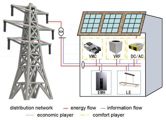
Figure 1.
Smart Building Structure Diagram.
3.1. Modeling of the VRF System
The VRF system discussed here is limited to a two-pipe system, where one outdoor unit is connected to multiple indoor units and all indoor units operate simultaneously in either cooling or heating mode.
The operating power of a VRF system is primarily determined by the seasonal coefficient of performance (SCOP) of the unit. The is defined as the ratio of cooling or heating capacity to operating power [16], as expressed in Equation (1):
Typically, the is not constant and reaches its maximum value when the load rate is between 50% and 70%. The value is determined by the outdoor temperature and the part load ratio (PLR) of the VRF outdoor unit, as expressed in Equation (2):
This paper, referring to reference [17], establishes the indoor thermal balance relationship as shown in Equation (3):
3.2. Modeling of the EWH
Consider a storage-type EWH. During the heating cycle, the main circuit is powered at a constant power level, i.e., the rated power. When not heating, only the control loop is used to monitor the temperature inside the EWH, with the power being negligible. The EWH outlet is equipped with a thermostat valve, and the water flow is constant in both flow and temperature, with heating maintained during the water release period. The thermodynamic dynamic process can be described by Equations (4)–(6) [5,18].
When the EWH is in heating mode, the temperature of the hot water inside the EWH is influenced by the heating power of the EWH and the ambient temperature, as shown in Equation (4):
When the EWH is in standby mode, the temperature of the water inside the tank is only affected by the external temperature, as shown in Equation (5):
When the user consumes hot water, a certain amount of cold water is injected into the bottom of the EWH tank to ensure an adequate water supply. At this point, the water temperature inside the tank should be adjusted, as shown in Equation (6):
3.3. Modeling of the VMC System
The VMC system consists of a centralized fresh air unit and a fan filtration unit, which are capable of delivering fresh outdoor air into the building while expelling indoor air. By considering only the ventilation function of the fresh air unit and applying the mass balance method, a VMC model is established based on the indoor/outdoor concentration of and airflow, as shown in Equations (7)–(9) [19]:
3.4. Modeling of the Lighting System
The indoor illuminance is mainly composed of two parts: indoor natural light illuminance and indoor lighting device illuminance . The former is mainly related to building structure, orientation, and other factors, while the latter is influenced by factors such as the type of light sources in the lighting system, the number of lamps, the room area, and the utilization factor of the fixtures. The total indoor illuminance can be calculated using Equations (10)–(12) [20]:
3.5. Modeling of Distributed Photovoltaic Equipment
The output power of the photovoltaic (PV) panel is related to solar radiation intensity, the area of the PV panel exposed to sunlight, and the photovoltaic panel’s photoelectric conversion efficiency. The photovoltaic system model is shown in Equations (13) and (14):
4. Evaluation of Multi-Dimensional Comfort for Building Occupants
Buildings are user-centered complex systems. They influence residential user comfort in more aspects than just air temperature. Factors such as domestic hot water, ambient lighting, and air quality also significantly affect human comfort. To address this, this paper proposes a multi-comfort model that considers thermal, lighting, and IAQ factors for users.
4.1. Visual Comfort
Numerous factors influence visual comfort, including light intensity, color temperature, brightness, and glare. In daily office environments, illuminance and color temperature play a predominant role. This study collects illuminance data from office buildings through direct measurements. It then uses statistical methods to analyze the quantitative relationship between visual comfort and lighting conditions. Additionally, it integrates users’ objective physiological responses to develop a visual comfort model.
4.1.1. Setting up the Experimental Scenario
The FLUKE941 illuminance meter (Fluke Corporation, Everett, WA, USA) is used to measure the illuminance values within the laboratory, with a measurement range of 0.1–100,000 lx. According to the measurement method described in reference [21], the floor is divided into a 1 m × 1 m grid. The center-point method is employed to measure the working surface illuminance values at each grid point:
4.1.2. Measured Average Illuminance
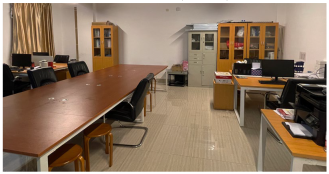
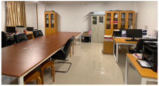
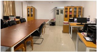
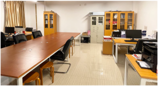
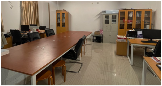
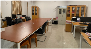
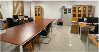
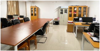
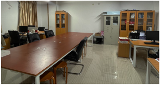
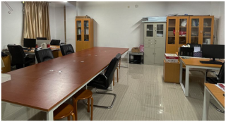
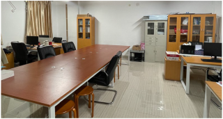
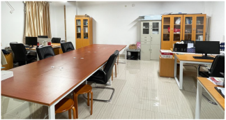
The experimental office was equipped with Philips double-ended LED T5 tubes, each with a power rating of 22 W and a luminous flux of 2300 lm. To ensure the validity and accuracy of the experiment, three color temperature models were selected, 6500 K, 4000 K, and 3000 K, to simulate various lighting conditions. The test site and spatial scenario schematic are shown in Table 1.

Table 1.
Illuminance Research Experimental Conditions Scenario.
4.1.3. Visual Comfort Evaluation Experiment
Since factors such as task type, individual differences, the experimental environment, experimental products, and time can influence the results, various measures were considered to ensure consistency and validity.
Because task type, individual differences, the indoor environment, products, experimental time, and other factors would have an influence on the results, a variety of measures were considered to ensure the consistency and effectiveness of the results. The visual comfort in an office environment is tested. First, in order to reduce the impact of individual differences, in this experiment, volunteers were recruited randomly from university, company, and residential communities. The conditions for selecting participants were as follows: (1) corrected vision ≥ 4.8 (E visual acuity chart); (2) did not wear photochromic glasses; (3) did not have a color vision deficiency (verified by the Ishihara test); and (4) no professional experience in lighting design or visual perception research. Finally, 30 participants (15 females and 15 males, aged between 20 and 50 years old) were involved in this experiment.
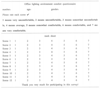
In terms of the experimental environment, in order to eliminate the influence of natural light, the entire experiment was carried out without natural light. The experimental room was a 90-square-meter office with white-painted ceilings and walls and white ceramic tile flooring, resembling most office environments in the country. The lighting fixtures were of the same model and series from the same manufacturer, with only the luminous flux varying, while all other parameters were identical, ensuring the scientific rigor and validity of the experiment. Prior to each experiment, participants underwent a 15 min adaptation period, after which they rated the experimental scene based on their subjective psychological perceptions. This step was repeated until all 24 experimental conditions had been evaluated. The experiment was scheduled to take place in the morning, afternoon, and evening to eliminate the influence of different times of day on the participants’ visual and psychological responses. Finally, the Likert scale was used to assess the participants’ subjective psychological perceptions [22].
The survey questionnaire and experimental scenario conditions are shown in Table 2.
Table 2.
Survey Questionnaire and Experimental Conditions.
4.1.4. Results, Statistics, and Analysis
To verify the consistency among participants and determine whether significant errors occurred during the evaluation process, Kendall’s coefficient of concordance test was applied to the experimental data. The specific calculation formula is shown in Equation (16).
After calculating the W value, the chi-squared test is used to determine its significance level for consistency. The specific formula is shown in Equation (17):
Kendall’s W coefficient calculation results obtained using SPSS software (version 30.0.0) are shown in Table 3.
Table 3.
Kendall Test.
According to the chi-squared critical value table, for large samples (K ≥ 20), Kendall’s W coefficient approximately follows a chi-squared distribution with (N − 1) degrees of freedom, denoted as . When the degrees of freedom, , and the significance level are less than 0.005, should be greater than 42.7956. Based on the experimental data in Table 3, it can be concluded that the participants’ ratings exhibit a high degree of consistency, and the experimental results are accurate and reliable.
Based on the correlated color temperature requirements for office spaces outlined in reference [23], a second-degree mathematical model was applied using SPSS software. Under an indoor color temperature of 4000 K, the average illuminance on the work surface and the visual comfort ratings were mathematically fitted, resulting in the expression shown in Equation (18).
In this equation, represents the visual comfort function, with a value range of 0–1, where 0 indicates the worst comfort level and 1 indicates the best comfort level. Figure 2 shows the curve of visual comfort variation with indoor illuminance.
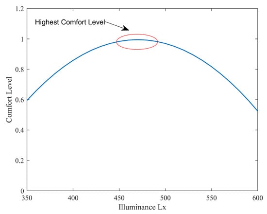
Figure 2.
Visual Comfort Level Variation with Illuminance.
4.2. Thermal Environment
In building environment comfort studies, the assessment of the thermal environment typically relies on indicators such as PMV (predicted mean vote) and PPD (predicted percentage of dissatisfied), which depend on specific measurements of temperature, humidity, wind speed, and radiant heat. However, in practical applications, these are often difficult to quantify accurately, especially when calculating radiant heat and estimating wind speed, where empirical constants are commonly used to simplify calculations. Therefore, this paper considers the temperature regulation capability of VRF and establishes a thermal environment indicator based on the optimal comfort temperature deviation and national standard constraints.
By optimizing control strategies, the upper and lower bounds of equipment setpoints are adjusted to improve electricity efficiency. The relationship between the thermal environment index and the setpoint temperature is expressed in Equation (19).
Human sensitivity to air temperature varies. When the temperature difference is small, sensitivity to temperature changes is low; when the temperature difference is large, sensitivity to temperature changes is high. Therefore, within the set temperature range, the greater the deviation from the optimal temperature, the lower the user’s comfort. The expression for the thermal environment is shown in Equations (20) and (21).
According to reference [24], the optimal indoor comfort temperature range is set between 22.9~26.6 °C, while the adjustable temperature range for the air conditioning equipment is set between 18~30 °C. Based on this, the curve of thermal environment variation with temperature is shown in Figure 3.
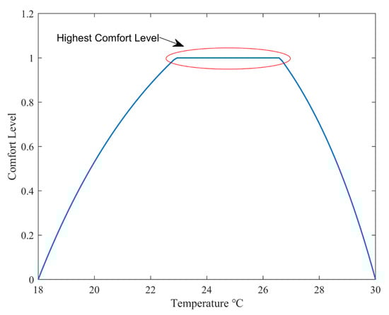
Figure 3.
Variation of Comfort Level with Temperature.
4.3. Water Comfort
The optimization goal of domestic hot water is to keep the water temperature as close as possible to the user-defined set point. Therefore, the difference between the optimal set water temperature and the actual temperature during all scheduled periods is used as the water comfort. The expression for water comfort is shown in Equations (22)–(24).
According to reference [25], the water comfort range is set between 35~45 °C. When the EWH uses municipal tap water, the lower limit of the hot water temperature is set to 20 °C. When the EWH is in full power heating mode, the upper limit of the hot water temperature is set to 60 °C. Based on this, the curve of water comfort variation with water temperature is shown in Figure 4.
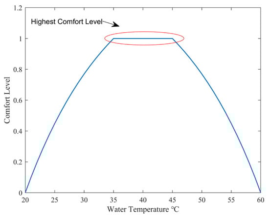
Figure 4.
Comfort Level of Hot Water as a Function of Water Temperature.
4.4. Indoor Air Quality
In indoor environments, factors such as PM2.5, , and CO affect air quality. Among these, concentration is the primary indicator for evaluating air quality. By monitoring the concentration, the comfort of residents can be assessed, and adjustments can be made to the VMC system. Based on actual data calculations and data fitting, the relationship between indoor concentrations and user satisfaction with the air quality is given by the curve shown in Equation (25) [26].
An expression for comfort, considering the actual IAQ range, is established, as shown in Equations (26) and (27):
According to reference [27], an indoor concentration not exceeding 1000 ppm (0.10%) per hour is considered normal. When the indoor concentration exceeds the normal level and reaches 2200 ppm, people may experience health issues such as a lack of concentration and mental fatigue. Therefore, the maximum adjustment limit is set to 2200 ppm. The curve of IAQ variation with concentration is shown in Figure 5.
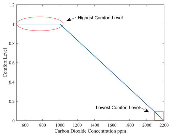
Figure 5.
Variation of IAQ Level with CO2 Concentration.
5. Non-Cooperative Game Strategy of Virtual Players Considering Multi-Comfort and Economic Goals
To avoid the potential impact of subjective decision-making in solving multi-objective problems, this paper constructs a virtual player-based non-cooperative game model centered on multi-comfort and economic objectives. By introducing new variables and constraints, the objective function is transformed into a differentiable convex form. Subsequently, the Nikaido–Isoda method is used to restructure the objective function, and the reconstructed game model is solved using the particle swarm optimization algorithm.
5.1. Payoff Functions
This paper constructs a non-cooperative game model with two virtual players, where the economic goal and the comfort goal serve as the objectives for the two virtual players, respectively. The economic objective function and the comfort objective function represent the payoff functions of the two virtual players.
- (1)
- Payoff function of the economic player:
- (2)
- Payoff function of the comfort virtual player:
5.2. Strategy Space
Research has indicated that the energy consumption of air conditioning systems in office buildings accounts for more than 50% of the building’s total energy consumption, making air conditioning systems the primary energy-consuming equipment. Considering the actual installation numbers of VRF, EWH, VMC, and LE systems, and based on the equilibrium and equivalence principle of the virtual player’s strategy space, the constraints of VRF devices and VMC systems are divided into the economic player’s strategy space. This is represented by Equations (1)–(3), (7)–(9), (13) and (14). The comfort player’s strategy space consists of the constraints of EWH devices, LE, and other devices, represented by Equations (4)–(6) and (10)–(12).
5.3. Converting the Payoff Function to a Differentiable Convex Form
Due to the presence of absolute value terms in Equation (30), the payoff function is non-differentiable and does not satisfy the conditions for a unique Nash equilibrium in non-cooperative games. Therefore, it is necessary to replace the original non-differentiable and non-convex payoff function with a differentiable quasi-convex function by introducing new constraints and variable substitutions. As shown in Equation (32), A and B are the newly introduced variables, and Equations (33)–(35) represent the corresponding additional constraints for these variables.
- (1)
- When is negative, can only be positive or zero to satisfy the constraint. To minimize the objective function, must be zero;
- (2)
- When is positive, can only be positive to satisfy the constraint. To minimize the objective function, must be positive;
- (3)
- When is zero, can only be positive or zero to satisfy the constraint. To minimize the objective function, must be zero.
- (4)
- Since represents the positive value of the electricity purchase quantity (with non-positive time values set to zero), the constraint involves negative values within the scheduling period (with non-negative time values set to zero). To minimize the objective function, they must be equal, representing the negative values within the scheduling period (with non-negative time values set to zero).
In summary, by adding new constraints and replacing variables, the absolute value term is eliminated, transforming the originally non-differentiable non-convex payoff function into a differentiable quasi-convex function, thus satisfying the conditions for a Nash equilibrium solution.
5.4. Reconstructing Payoff Functions Using the Nikaido–Isoda Method
Directly solving the Nash equilibrium solution for the non-cooperative game model of economic efficiency and comfort involves high computational complexity and convergence difficulties in the optimization results. To reduce computational complexity, this study introduces a regularized Nikaido–Isoda function, transforming the game problem into a global optimization problem of finding the maximum–minimum value [28].
The Nikaido–Isoda function is a key function for Nash equilibrium analysis. For different strategies x and y within the same strategy set, it is expressed as shown in Equation (36):
In this equation, represents the payoff function of virtual player v; and are the strategy of virtual player u and the strategies of all other players except v, respectively; and represents the modified strategy of virtual player v.
From the above equation, it can be seen that the primary meaning of the Nikaido–Isoda function is to describe the change in total payoff when the strategy of virtual player v changes while the strategies of other participants remain unchanged. After regularization, it can be expressed as:
In this equation, is a constant coefficient greater than zero.
The function is defined as shown in Equation (38):
In this equation, represents the function expression after transforming the original non-cooperative game problem into a global optimization problem. The condition appears if and only if (where is the optimal strategy) satisfies the Nash equilibrium. For the detailed proof, refer to [29]. Therefore, solving for the Nash equilibrium can be equivalently transformed into solving a global optimization problem.
Substituting the payoff functions in Equations (28) and (31) into Equation (38) yields:
In this equation, and represent the payoff functions of the economic virtual player and the comfort virtual player, respectively. and denote the adjusted equipment outputs during time period t; and and represent the modified equipment output scheduling strategies.
5.5. Solution Method
To solve the non-cooperative game model, compared to conventional methods, intelligent algorithms have the advantages of strong global search capabilities and fast convergence. To improve global optimization performance in solving the non-cooperative game model, the PSO algorithm is used. The parameters for the PSO algorithm are set as follows: 300 particles and 150 iterations, with both the individual learning factor and the global learning factor set to 1.55. The initial inertia factor is set to 0.95, and the final inertia factor is set to 0.5. The algorithm flow is shown in Figure 6, and the specific steps for solving are as follows:
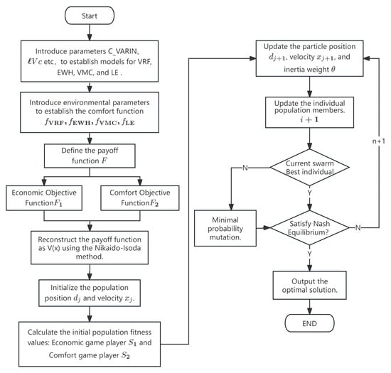
Figure 6.
Flowchart of the Non-Cooperative Game Model Solution.
Step 1: Input the initial data and parameters of the system, including outdoor light intensity, outdoor temperature, and predicted outputs of wind and photovoltaic power.
Step 2: Initialize the strategies of the virtual players, i.e., initialize the starting strategies for the economic virtual player and the comfort virtual player.
Step 3: To ensure the existence of a Nash equilibrium solution in the game model, use auxiliary variables to transform the payoff functions into differentiable quasi-convex functions. Combine the Nikaido–Isoda function with regularization to reconstruct the payoff functions, thereby obtaining the global optimal model, which facilitates the acquisition of the Nash equilibrium solution.
Step 4: Each game participant optimizes individually. According to the definition of a Nash equilibrium, each participant optimizes their strategy in the i round based on the strategy of the other participant in the i − 1 round, with the goal of maximizing their own payoff function. The mathematical expression for the optimal strategy in the i round is given in Equation (40).
Step 5: Determine whether a Nash equilibrium point has been found. If the strategies in two consecutive rounds are identical, i.e., satisfy Equation (41), it indicates that a Nash equilibrium point has been found. Each game participant then configures their capacity according to the strategy at this point and calculates their own payoff function. Otherwise, return to step 4.
Step 6: Output the Nash equilibrium point and the payoff functions and .
6. Simulation and Results Analysis
This study selects a three-story office building in North China as the research object. The building has a usable area of approximately 10,000 , equipped with energy-consuming devices including VRF, EWH, VMC, and LE systems. The total scheduling duration is set for 24 h of a typical day in summer and winter. The photovoltaic power generation curves and outdoor temperatures for typical summer and winter days are shown in Appendix A Figure A1 and Figure A2.
The operating parameters of the VRF, EWH, VMC, and LE systems involved in scheduling optimization are presented in Table 4. According to reference [30], the daylight factor for public buildings is set to a standard value of 2%, and the lighting method adopts uniform illumination. The natural indoor lighting intensity curves for typical summer and winter days in the building are shown in Appendix A, Figure A3. The time-of-use electricity pricing and electricity selling price data used in this study are derived from the “2023 Time-of-Use Electricity Pricing Announcement for Industrial and Commercial Sectors” issued by the China Shandong State Grid Electricity Corporation.
Table 4.
Equipment Operating Parameters.
6.1. Simulation Scenarios
In order to thoroughly assess the validity and applicability of the adjustment strategies, five comparative scenarios are established as follows:
Scenario 1: Optimization of the building energy system’s equipment output scheduling, considering only economic objectives.
Scenario 2: Optimization of the building energy system’s equipment output scheduling, considering only comfort objectives.
Scenario 3: Optimization of the building energy system’s output scheduling by considering both economic objectives and multiple comfort objectives. The problem is solved using the NSGA-II.
Scenario 4: Optimization of the building energy system’s output scheduling by considering both economic objectives and multiple comfort objectives. A weighted method is used to transform the multi-objective problem into a single-objective problem for solving.
Scenario 5: Optimization of the building energy system’s output scheduling by considering both economic objectives and multiple comfort objectives. A non-cooperative game model is established between economic virtual players and comfort virtual players, and the problem is solved accordingly.
6.2. Optimization Results Analysis
Based on the five scenarios defined above, Scenario 3 employs the NSGA-II algorithm for optimization, with the population size set to 300 and the number of iterations fixed at 300. Scenario 5 constructs a non-cooperative game model for virtual players, which is solved using intelligent algorithms. The iterative convergence trend is shown in Figure 7.
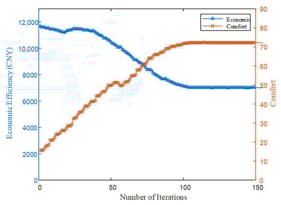
Figure 7.
Iterative Convergence Curve of the Economic Game Player in Scenario 5.
Figure 7 illustrates the iterative convergence curves of the non-cooperative game in Scenario 5. On the left, the total economic cost of the VRF, EWH, VMC, and LE systems is depicted, while the right shows the overall comfort level, the thermal environment, water comfort, IAQ, and visual comfort. During the iterations, the payoff function of the economic virtual player demonstrates a gradual downward trend, whereas the payoff function of the comfort virtual player shows a gradual upward trend. By the 110th iteration, the economic and comfort virtual players reach a stable equilibrium.
Table 5 presents the numerical results of economic performance and overall comfort for the coordinated optimization scheduling of equipment output adjustment models across Scenarios 1 to 5 under different strategies. In Scenario 1, which considers only economic cost, the economic value is the lowest, while Scenario 2, which prioritizes comfort, achieves the highest overall comfort value. Scenario 5 surpasses Scenario 4 in both economic and comfort metrics, confirming that the Nash equilibrium solution obtained in this study effectively balances the objectives of economy and comfort. Numerically, the economic cost in Scenario 5 is reduced by CNY 549 compared to Scenario 3 and by CNY 288 compared to Scenario 4. In terms of comfort, Scenario 5 improves the comfort level by 31.45% compared to Scenario 4. Therefore, the model established in this study is meaningful, as the result represents a stable outcome of the two-objective game.
Table 5.
Comparison of Multi-Scenario Optimization Objectives.
Figure 8 depicts the indoor temperature fluctuations of VRF equipment on a typical summer day in Scenarios 1 and 5. In Scenario 1, the operation scheduling of the VRV system is solely based on economic considerations. The VRV system initiates cooling when the indoor temperature exceeds 28.2 °C, resulting in a decrease in indoor temperature. In contrast, Scenario 5 takes into account both economic factors and comfort levels. The VRV system activates cooling when the indoor temperature surpasses 26.3 °C, which is beyond the comfort range, leading to a reduction in indoor temperature. When the indoor temperature is between 26.3 °C and 22.9 °C, within the comfort range, the VRV system ceases operation, thereby reducing energy consumption and operational costs. Unlike Scenario 1, Scenario 5 dynamically adjusts the operational status of the VRV system, significantly enhancing user thermal comfort at the expense of a certain degree of economic efficiency. This ensures a balance between economic benefits and thermal comfort for the users.
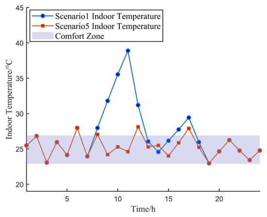
Figure 8.
Time-Varying Indoor Temperature Curves for Scenario 1 and Scenario 5.
Figure 9 illustrates the hot water temperature variation curve of the EWH system on a typical summer day in Scenario 5. In this case study, the user’s summer comfort temperature range is set between 36.5~42.1 °C. As shown in the figure, the EWH system preheats the water in the tank at 3:00 and 15:00 to ensure sufficient hot water for user needs. In the subsequent time periods following heating, the water temperature decreases rapidly. This occurs primarily because the EWH system reaches the upper temperature limit, causing it to enter a heat preservation state. When users consume hot water, a certain amount of cold water is automatically added to maintain sufficient tank capacity. During this process, the water temperature decreases, prompting the EWH system to resume heating.
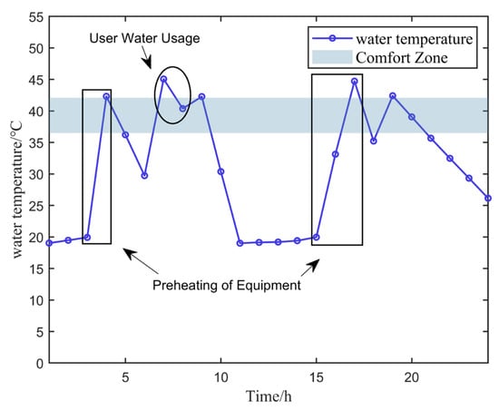
Figure 9.
Diurnal Variation of Hot Water Temperature in Scenario 5.
Figure 10 shows the variation curve of the indoor concentration of the VMC system on a typical summer day in Scenario 5. In the case study, there are eight people active in a room from 8:00–13:00 on workdays, and eleven people active from 15:00–22:00 on workdays, with no activity during other times. When there are no occupants in the room, the VMC system operates at a low power setting, resulting in lower energy consumption. As the number of people in the room increases and the indoor concentration rises above 1100 ppm, the VMC system switches to a high-power setting. This allows the concentration to drop rapidly, maintaining the indoor levels within a normal range.
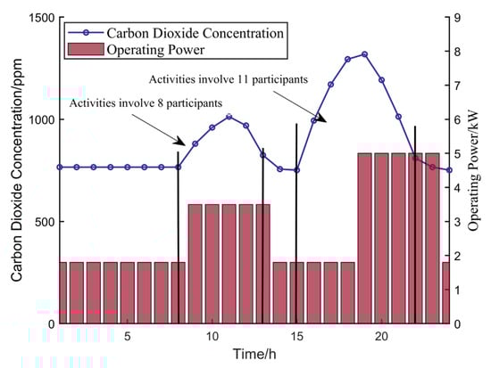
Figure 10.
Diurnal Variation of Indoor CO2 Concentrations in Scenario 5.
Figure 11 shows the output and user comfort variation of LE in Scenario 1 and Scenario 5 on a typical summer day. During the early and late summer hours, when natural indoor light intensity is relatively low, user comfort tends to be generally low when the LE is off. In Scenario 1, which considers only economic performance, the lighting system always operates at the lowest power setting, sacrificing user comfort to reduce electricity costs. In Scenario 5, which simultaneously considers both comfort and economy, the lighting system adjusts its operating state and different power levels based on the intensity of natural indoor light. This ensures that the indoor illumination remains within a range that provides higher visual comfort for the user.
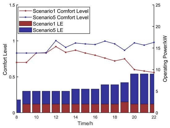
Figure 11.
Diurnal Variation of Visual Comfort Levels in Scenario 1 and Scenario 5.
Figure 12 shows the variation curves of multi-device output and overall comfort in Scenario 5. From 0:00–8:00 on workdays, the devices generally maintain a low output, resulting in lower energy consumption but poorer comfort. Between 8:00–13:00 and 16:00–22:00, most equipment operates at peak output, coinciding with the highest number of office building occupants. During this period, user comfort levels fluctuate between 2~3, effectively ensuring comfort while reducing equipment operating costs.
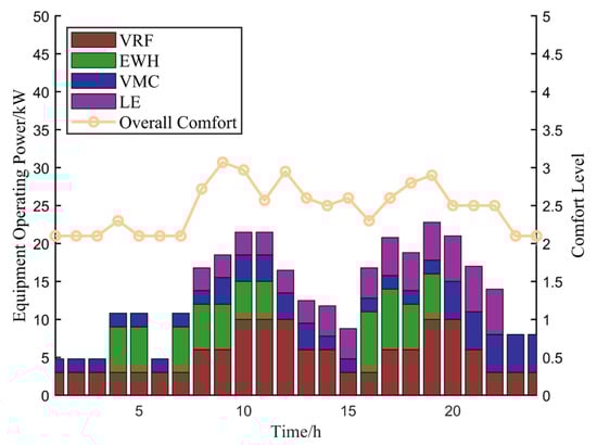
Figure 12.
Variation Curve of Equipment Output and Comfort Level in Scenario 5.
7. Conclusions
This study focuses on the major electrical devices in office buildings. It first establishes physical models for these devices and analyzes user comfort requirements, developing a multi-dimensional comfort expression for thermal, lighting, and IAQ factors. Considering the subjective processes involved in conventional methods for solving multi-objective problems, a non-cooperative game model with a single virtual player was proposed, using economic and comfort objectives. The corresponding solving algorithm was applied, and the results for user comfort variations, device scheduling, and operational costs for a typical summer day were obtained, showing the following conclusions:
- (1)
- Based on load operation characteristics, the main electrical devices in buildings were categorized, and detailed physical models for VRF, EWH, VMC, and LE were established. This work lays the foundation for subsequent non-cooperative game scheduling strategies.
- (2)
- A comprehensive analysis of multiple comfort factors was conducted. For visual comfort, a fitting expression between the average illuminance of the working plane and the comfort rating was developed. IAQ and the thermal environment were modeled by using the difference between the standard set values and the actual temperature as the comfort deviation, establishing a multi-dimensional comfort expression. The integrated comfort expression developed here better reflects actual user comfort conditions and more comprehensively satisfies user comfort needs.
- (3)
- A scheduling strategy was established that simultaneously considers user economy and various comfort factors. This strategy involves non-cooperative game scheduling for the economic virtual player and the comfort virtual player. Through case studies, it was verified that compared to the particle swarm optimization algorithm, the scheduling strategy used in this paper reduced economic costs by 3.89% and improved comfort by 31.45%, effectively enhancing user comfort while reducing energy costs.
There are still some limitations to this study. In terms of the visual comfort experiment, differences in perceptions of light among different age groups (e.g., young and elderly individuals) were not considered, which may lead to the insufficient adaptability of results. Additionally, the simulation only focused on a typical daily load scenario in summer, without performance evaluation in other seasons and under extreme climate conditions.
Future research could further model differentiated comfort functions, such as modifying comfort demands based on age and occupation. It could also integrate objective physiological indicators (e.g., pupil response and electroencephalogram) with subjective score data and enhance the model validation process to ensure the reliability of the developed model. Furthermore, simulations should be expanded to cover a variety of climate scenarios throughout the year to verify the environmental robustness and generalization capabilities of the optimization strategy.
Author Contributions
Conceptualization, Z.F.; methodology, Z.F.; software, Q.Y.; validation, X.B.; formal analysis, Z.F.; investigation, Q.Y.; resources, R.W.; data curation, Q.Y.; writing—original draft preparation, Z.F.; writing—review and editing, X.B.; visualization, X.B.; supervision, R.W.; project administration, R.W.; funding acquisition, X.B. All authors have read and agreed to the published version of the manuscript.
Funding
Taishan Industrial Experts Programme (No. tscx202312127); Shandong Province Transportation Planning and Design Institute Group’s Science and Technology Innovation Project (No. KJ-2023-SJYJT-06).
Data Availability Statement
Data are contained within the article.
Conflicts of Interest
Author Xiyong Bao was employed by the company Shandong Provincial Communications Planning and Design Institute Group Co., Ltd. Author Ruiqi Wang was employed by the company State Grid Shandong Integrated Energy Services Co., Ltd. The remaining authors declare that the research was conducted in the absence of any commercial or financial relationships that could be construed as a potential conflict of interest.
Nomenclature
| Operating power of the VRF | kW | |
| Energy Efficiency Ratio of the VRF | - | |
| Cooling/heating capacity for indoor unit w | J | |
| Number of VRF Indoor Units | - | |
| Rated cooling capacity of VRF outdoor unit | kW | |
| Thermal difference heat gain coefficient | - | |
| Heat capacity heat gain coefficient | - | |
| Outdoor temperature at time t | °C | |
| Indoor temperature at time t | °C | |
| Room heat capacity | J/K | |
| Indoor set temperature | °C | |
| Indoor heat source power | W | |
| Hot water temperature of EWH at time t | °C | |
| EWH heating power | kW | |
| Switch status of EWH at time t | - | |
| EWH insulation performance coefficient | - | |
| Density of Water | g/L | |
| Specific heat capacity of Water | ||
| Water tank volume | m3 | |
| Inlet water temperature of EWH | °C | |
| The amount of cold water injected at time t | L | |
| Indoor concentration at time t | ppm | |
| Outdoor concentration at time t | ppm | |
| The concentration generated at time t. | ppm | |
| Initial indoor concentration. | ppm | |
| Indoor space volume. | m3 | |
| Ventilation airflow of VMC at time t. | m3 | |
| Ventilation rate during VMC operation. | m3/h | |
| The Energy Efficiency Ratio of VMC. | - | |
| VMC operating power at time t | kW | |
| The illuminance at time t | lx | |
| DF | Daylight factor | - |
| Outdoor illuminance at time t | lx | |
| U | Lighting utilization factor | - |
| Luminous flux of LE | lm | |
| n | Number of lighting circuits | - |
| Rated power of the light fixtures | W | |
| S | Lighting area | m2 |
| The output power of photovoltaic equipment at time t | kW | |
| Photovoltaic solar panel area | m2 | |
| Photoelectric conversion efficiency | - | |
| Solar radiation at time t | kW/m2 | |
| Average illuminance on the work surface | lx | |
| Illuminance at measurement point i | lx | |
| N | Number of Experiments | - |
| K | Number of Experiment volunteers | - |
| Total Score of the i-th Experiment | - | |
| Adjustable lower limit of Indoor temperature | °C | |
| Adjustable lower limit of outdoor temperature | °C | |
| Optimal upper temperature limit | °C | |
| Optimal lower temperature limit | °C | |
| Thermal comfort index at time t | - | |
| Thermal comfort expression | - | |
| Switch status of VRF at time t | - | |
| Water comfort index | - | |
| Water comfort expression | - | |
| Switch status of EWH at time t | - | |
| Adjustable upper limit of EWH temperature | °C | |
| Adjustable lower limit of EWH temperature | °C | |
| IAQ Index at time t | - | |
| IAQ expression | - | |
| Adjustable upper limit of indoor concentration | ppm | |
| Adjustable lower limit of indoor concentration | ppm | |
| Most comfortable concentration | ppm | |
| System operation and maintenance cost | RMB | |
| System purchase and sale energy cost | RMB | |
| m | Total number of devices | - |
| Operation and maintenance cost of VRF, VMC, and other devices | RMB | |
| Output power of device k at time t | kW | |
| Time-of-Use electricity price | RMB | |
| Electricity selling price | RMB | |
| Power interaction between the system and the grid | kW |
Appendix A
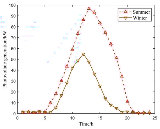
Figure A1.
Photovoltaic generation curves for typical summer and winter days.
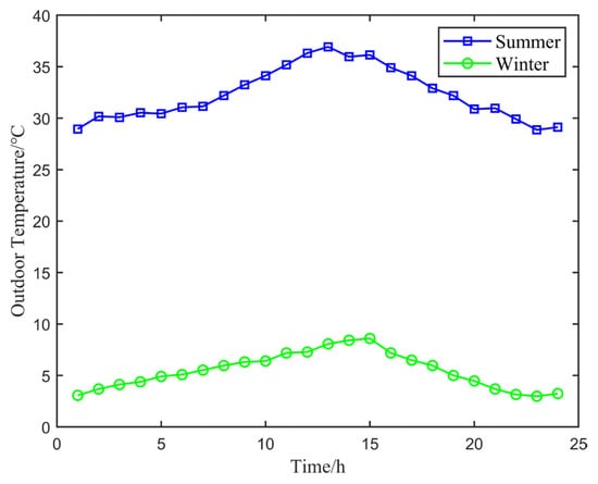
Figure A2.
Outdoor temperature curves for typical summer and winter days.
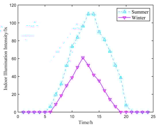
Figure A3.
Typical daily indoor natural illumination intensity variation curves for summer and winter seasons.
References
- Hou, X.; Wang, J.; Huang, T.; Wang, T.; Wang, P. Smart home energy management optimization method considering energy storage and electric vehicle. IEEE Access 2019, 7, 144010–144020. [Google Scholar] [CrossRef]
- Wu, X.; Li, Y.; Tan, Y.; Cao, Y.; Rehtanz, C. Optimal energy management for the residential MES. IET Gener. Transm. Distribution 2019, 13, 1786–1793. [Google Scholar] [CrossRef]
- Lv, G.; Cao, B.; Dexiang, J.; Wang, N.; Li, J.; Chen, G. Optimal scheduling of regional integrated energy system considering integrated demand response. CSEE J. Power Energy Syst. 2021, 10, 1208–1219. [Google Scholar]
- Yang, X.; Fu, G.; Liu, F.; Tian, Y.; Xu, Y.; Chai, Z. Potential evaluation and control strategy of air conditioning load aggregation response considering multiple factors. Power Syst. Technol. 2022, 46, 699–714. [Google Scholar]
- Bhandari, N.; Tadepalli, S.; Gopalakrishnan, P. Investigation of acoustic comfort, productivity, and engagement in naturally ventilated university classrooms: Role of background noise and students’ noise sensitivity. Build. Environ. 2024, 249, 111131. [Google Scholar] [CrossRef]
- Latif, M.; Nasir, A. Decentralized stochastic control for building energy and comfort management. J. Build. Eng. 2019, 24, 100739. [Google Scholar] [CrossRef]
- Liu, Y.; Yu, J.Y.; Yu, G. Stdies on Light and Heat Environment and Comfort Evaluation of Living Space of the Disabled Elderly in the Existing Residence. J. Hum. Settl. West China 2021, 36, 31–39. [Google Scholar]
- Wu, J.; Wang, H.; Wang, W.; Zhang, Q. Performance evaluation for sustainability of wind energy project using improved multi-criteria decision-making method. J. Mod. Power Syst. Clean Energy 2019, 7, 1165–1176. [Google Scholar] [CrossRef]
- Qu, Z.; Qu, N.; Liu, Y.; Yin, X.; Qu, C.; Wang, W.; Han, J. Multi-objective optimization model of electricity behavior considering the combination of household appliance correlation and comfort. J. Electr. Eng. Technol. 2018, 13, 1821–1830. [Google Scholar]
- Li, J.; Wang, Z.; Yan, S.; Wang, C.; Bao, L.; Qin, H. Optimal operation of home energy management system considering user comfort preference. Acta Energiae Solaris Sin. 2020, 41, 51–58. [Google Scholar]
- Wang, S.; Dong, Y.; Zhao, Q.; Zhang, X. Bi-level multi-objective joint planning of distribution networks considering uncertainties. J. Mod. Power Syst. Clean Energy 2021, 10, 1599–1613. [Google Scholar] [CrossRef]
- Cao, Y.; Wang, D.; Jia, H.; Lei, Y.; Li, J. Bilevel Nash-Stackelberg game expansion planning of regional integrated energy system considering multi-energy carbon flow constraints. Autom. Electr. Power Syst. 2023, 47, 12–22. [Google Scholar]
- Ilak, P.; Kuzle, I.; Herenčić, L.; Đaković, J.; Rajšl, I. Market power of coordinated hydro-wind joint bidding: Croatian power system case study. J. Mod. Power Syst. Clean Energy 2021, 10, 531–541. [Google Scholar] [CrossRef]
- Querini, P.L.; Chiotti, O.; Fernádez, E. Cooperative energy management system for networked microgrids. Sustain. Energy Grids Netw. 2020, 23, 100371. [Google Scholar] [CrossRef]
- Wang, Q.; Zeng, J.; Liu, J.F.; Chen, J.L.; Wang, Z.G. A distributed multi-objective optimization algorithm for resource-storage-load interaction of microgrid. Proc. CSEE 2020, 40, 1421–1431. [Google Scholar]
- Cheng, L.; Wan, Y.; Zhang, F. Operation mode and control strategy for air-conditioning service based on business of load aggregator. Autom. Electr. Power Syst. 2018, 42, 8–18. [Google Scholar]
- Li, Y.T.; Hao, B. Empirical study on flexible load of multi connected air conditioning participating in power system demand response. Distrib. Util. 2022, 39, 39–46. [Google Scholar]
- Chen, Z.; Li, Y.Q.; Leng, Z.Y.; Lu, G.X. Refined modeling and energy management strategy of typical household high-power loads. Autom. Electr. Power Syst. 2018, 42, 135–143. [Google Scholar]
- Berouine, A.; Ouladsine, R.; Bakhouya, M.; Essaaidi, M. Towards a real-time predictive management approach of indoor air quality in energy-efficient buildings. Energies 2020, 13, 3246. [Google Scholar] [CrossRef]
- Yelisetti, S.; Saini, V.K.; Kumar, R.; Lamba, R. Energy consumption cost benefits through smart home energy management in residential buildings: An indian case study. In Proceedings of the 2022 IEEE IAS Global Conference on Emerging Technologies (GlobConET), Arad, Romania, 20–22 May 2022; pp. 930–935. [Google Scholar]
- GB/T 5700-2023; Methods of Lighting Measurement. National Technical Committee for Ergonomics Standardization: Beijing, China, 2023.
- Lionello, M.; Aletta, F.; Mitchell, A.; Kang, J. Introducing a method for intervals correction on multiple Likert scales: A case study on an urban soundscape data collection instrument. Front. Psychol. 2021, 11, 602831. [Google Scholar] [CrossRef]
- GB/T 50034-2024; Standard for Lighting Design of Buildings. Ministry of Housing and Urban-Rural Development of the People’s Republic of China: Beijing, China, 2024.
- GB/T 50785-2012; Evaluation Standard for Indoor Thermal Environmentin Civil Buildings. Ministry of Housing and Urban-Rural Development of the People’s Republic of China: Beijing, China, 2012.
- GB 50368-2005; Residential Building Code. Ministry of Housing and Urban-Rural Development of the People’s Republic of China: Beijing, China, 2005.
- Yelisetti, S.; Saini, V.K.; Kumar, R. Data Driven Thermal Comfort Model For Smart Home Energy Management System. In Proceedings of the 2022 IEEE International Conference on Power Electronics, Drives and Energy Systems (PEDES), Jaipur, India, 14–17 December 2022; pp. 1–6. [Google Scholar]
- GB/T 18883-2022; Standards for Indoor Air Quality. National Health Commission of the People’s Republic of China: Beijing, China, 2022.
- Yang, J.; Tushar, W.; Saha, T.K.; Alam, M.R.; Li, Y. Prosumer-driven voltage regulation via coordinated real and reactive power control. IEEE Trans. Smart Grid 2021, 13, 1441–1452. [Google Scholar] [CrossRef]
- Zhang, G.Q.; Zhao, G.D. An Improved Differential Evolution Algorithm for Solving Nash Equilibrium Problem and Generalized Nash Equilibrium Problem. Oper. Res. Sci. 2023, 32, 36–42. [Google Scholar]
- GB 50033-2013; Standard for Daylighting Design of Buildings. Ministry of Housing and Urban-Rural Development of the People’s Republic of China: Beijing, China, 2013.
Disclaimer/Publisher’s Note: The statements, opinions and data contained in all publications are solely those of the individual author(s) and contributor(s) and not of MDPI and/or the editor(s). MDPI and/or the editor(s) disclaim responsibility for any injury to people or property resulting from any ideas, methods, instructions or products referred to in the content. |
© 2025 by the authors. Licensee MDPI, Basel, Switzerland. This article is an open access article distributed under the terms and conditions of the Creative Commons Attribution (CC BY) license (https://creativecommons.org/licenses/by/4.0/).