Investigation on Thermal Environment of Urban Slow Lane Based on Mobile Measurement Method—A Case Study of Swan Lake Area in Hefei, China

Abstract

Numerous issues with the urban thermal environment have been brought on by the rapid development of urbanization. The thermal climate of the slow lane, a major urban activity area, is directly tied to the well-being and comfort of city dwellers. The Swan Lake area in Hefei was chosen as the research site for this paper. The mobile measurement method was used to determine the heat island intensity distribution of the slow lane in each season of the year. The effects of building density, the percentage of permeable underlying surface, and shading on the slow lane’s thermal environment were then thoroughly examined. According to the study, the distribution of heat island intensities along the mobile measurement route varies significantly depending on season, as well as time of year. Summer and winter have the most notable variations in the distribution of heat island intensities along the mobile measurement route; the summer values range from 0.1 to 4, while the winter values range from −0.3 to 3. The results showed a maximum difference of 30.2 °C in surface temperature (Ts) readings and 11.9 °C in air temperature (Ta) readings between the identical sites with and without shading, according to tests conducted at four typical mobile measurement locations along the mobile measuring route. The shading factor has a greater effect on the slow lane’s thermal environment than permeable underlying surface and building density, as seen by the standardized coefficient of shading being significantly higher than both of these factors. With a standardized coefficient of shading of −0.493 in the winter and a standardized coefficient of shading of −0.517 in the summer, the effect of the shading factor on the thermal environment is more noticeable in the summer.

1. Introduction

The rapid growth of urbanization in the current atmosphere of global warming has resulted in an increasing amount of issues with the urban outdoor thermal environment [1,2,3]. Specifically, 38–40% of urban land cover comprises slow lanes, which are among the most crucial routes for short-distance transit [4]. Slow lanes are a vital type of urban space, closely tied to residents’ daily lives. Particularly, slow lanes within cities, as key components of the slow traffic system, connect communities and surrounding areas, offering higher usage frequency and a more direct experience [5]. The thermal environment of the slow lane exerts a more pronounced influence on pedestrians, with the study indicating a temperature rise of 1 °C in the hot summer conditions. Heat-related morbidity and mortality will rise by 1% to 3% [6], thus impacting public health [7,8,9]. Consequently, a comprehensive analysis of the underlying surface influence on the thermal conditions of the slow lane is crucial for alleviating the urban heat island effect and establishing a comfortable thermal environment through judicious urban planning.

The urban thermal environment is influenced by various elements, including the quantity of solar radiation received at the surface of the urban area and its conversion into sensible heat [10], urban physical characteristics (e.g., urban layout, type and structure of the underlying surface) [11,12,13], socio-economic aspects (e.g., land use) [14], and demographic attributes (e.g., age, income, and population density) [15,16]. The urban underlying surface is a factor determining alterations in the thermal environment [17,18,19]. The primary focus of the study is to analyze the effect of the underlying surface temperature on the thermal environment. Specifically, by examining the impact of subsoil type and pavement material on the slow lane temperature [20], it was determined that augmenting the natural subsoil cover within urban areas can mitigate the intensity of the urban heat island (UHI) effect and the likelihood of warming [21]. Furthermore, the detrimental influence of bare soil on the thermal environment ranks just below that of impervious slow lane. Additionally, it was observed that shading can markedly decrease the average radiant temperature [22], as shading facilitates the reduction of reflected longwave radiation from the ground. Furthermore, shading diminishes the reflection of longwave radiation from the ground [23]. Additionally, the cooling capacity of urban tree shading significantly influences the urban thermal environment [24,25]. However, numerous factors affect the thermal environment, and the mechanisms involved are intricate, with synergistic interactions being among these factors, complicating the analysis. The current analysis of the underlying surface’s impact on the thermal environment is limited, focusing solely on a single factor. Therefore, further investigation is required to examine the combined effects of the underlying surface, building density, and shading distribution on the urban thermal environment; thus, optimizing the urban heat island effect has become urgent.

Different underlying surface parameters play a key role in facilitating thermal mitigation strategies and human adaptation measures. Changes in urban land use patterns and morphological characteristics have significantly increased urban temperatures, resulting in higher temperatures in the city than in the suburbs, creating the urban heat island (UHI) [26]. The UHI directly or indirectly affects the thermal comfort and well-being of urban residents [27]. Consequently, an increasing number of researchers are focusing on the UHI and using it to assess and improve the urban thermal environment [28]. However, current research on the thermal environment of slow lanes has mainly focused on the effects of the geometry of the slow lanes on the microclimate generated [29], while there have been few comprehensive analyses on the effects of different underlying surface parameters on the intensity distribution of heat islands in slow lanes.

To address these limitations, researchers have proposed several methods. The current methodology for studying the impact of thermal environments relies on field observations and numerical simulations. Given the multitude of factors influencing the actual thermal environment, numerical simulations struggle to adequately account for the intricate effects of these variables. Consequently, contemporary research on urban thermal environments predominantly utilizes field testing [30], which encompasses fixed observations, mobile measurements [31], and remote sensing technologies [32]. The thermal environment data acquired through fixed observation methods are precise and reveal the dynamic fluctuation patterns of long-term testing [33]. However, the local spatial diversity and complexity necessitate that the study of the local thermal environment spatially encompasses as many representative locations as possible [34]. This approach would require substantial resources and a workforce for real-time monitoring via fixed meteorological stations. Furthermore, remote sensing technology is constrained by the complexity of the field surroundings and cannot adequately characterize the thermal environment of medium urban areas [35]. Remote sensing technology, constrained by the complexities of the field environment, fails to adequately characterize the thermal environment of urban small-scale areas. It offers only an instantaneous surface temperature distribution image, necessitating inversion of measurement data through the quantitative relationship with air temperature, which significantly impacts the accuracy of spatial thermal environment calculations at pedestrian height. In contrast, mobile measurement technology can acquire thermal environment parameters (e.g., air temperature and humidity) from several representative locations using a limited number of instruments, facilitating the analysis of the spatial and temporal distribution and characteristics of urban thermal environment parameters [36,37]. Mobile measurements can ascertain the temperature distribution in urban areas that are inaccessible to vehicles, as well as the temperature profiles of meteorological stations at monitoring points [38]. Additionally, mobile tests are more cost-effective for measuring and capturing gradual changes in thermal conditions that vary with the landscape [39]. Sundborg [40] (1951) was the first to employ mobile measurement in Sweden to investigate the urban heat island (UHI) effect; Mizuno M [41] and Leconte, F [42] (2015) examined the mechanism by which urban structure affects a city’s thermal climate by mobile measurement. Liu Lin [43] (2017) employed mobile measurement to investigate local-scale urban heat island (UHI) characteristics across various urban patterns; Cao C [44] (2020) utilized mobile measurement to examine the correlation between urban vegetation distribution and the mitigation of high humidity and temperature issues in Nanjing; and Emery, J [45] (2021) analyzed mobile measurement of air temperature in eastern France to assess the influence of urban form on micro-scale temperature variations. Chafer, M [46] (2022) examined the effects of various urban forms (e.g., high-rise and low-rise structures, green spaces) on the urban microclimate in Singapore, as well as the intensity of the urban heat island (UHI) effect associated with these forms, utilizing mobile measurements. In recent years, mobile measurements have been extensively utilized in thermal environment research.

This paper focuses on the Swan Lake area in Hefei City, examining the thermal environment of the slow lane using the mobile measurement method, primarily analyzing the effects of different underlying surface parameters on the pedestrian-level thermal conditions of the slow lane. Section 2 of this paper primarily delineates the study area and the measurement method. Section 3 initially evaluates the accuracy of four temporal correction models pertaining to the mobile measurement method. Subsequently, it examines the distribution of heat island intensity along the mobile measurement route across various seasons and times, as well as the shading distribution at typical locations on the mobile test route during different time intervals. It further investigates the resultant variations in surface and air temperatures, culminating in a comprehensive analysis of the thermal environment at varying pedestrian heights on the slow lane. The impact of varying building densities, proportions of the permeable underlying surface, and shading on the thermal conditions of the slow lane were also examined.

2. Materials and Methods

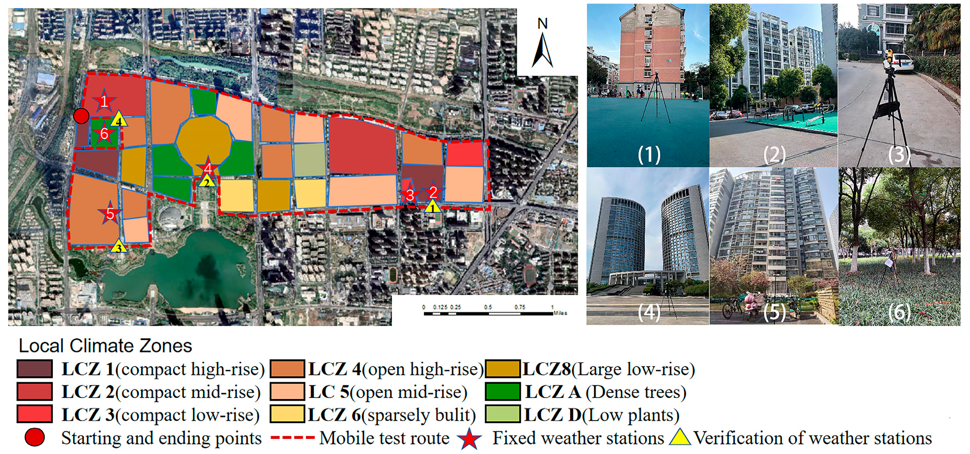
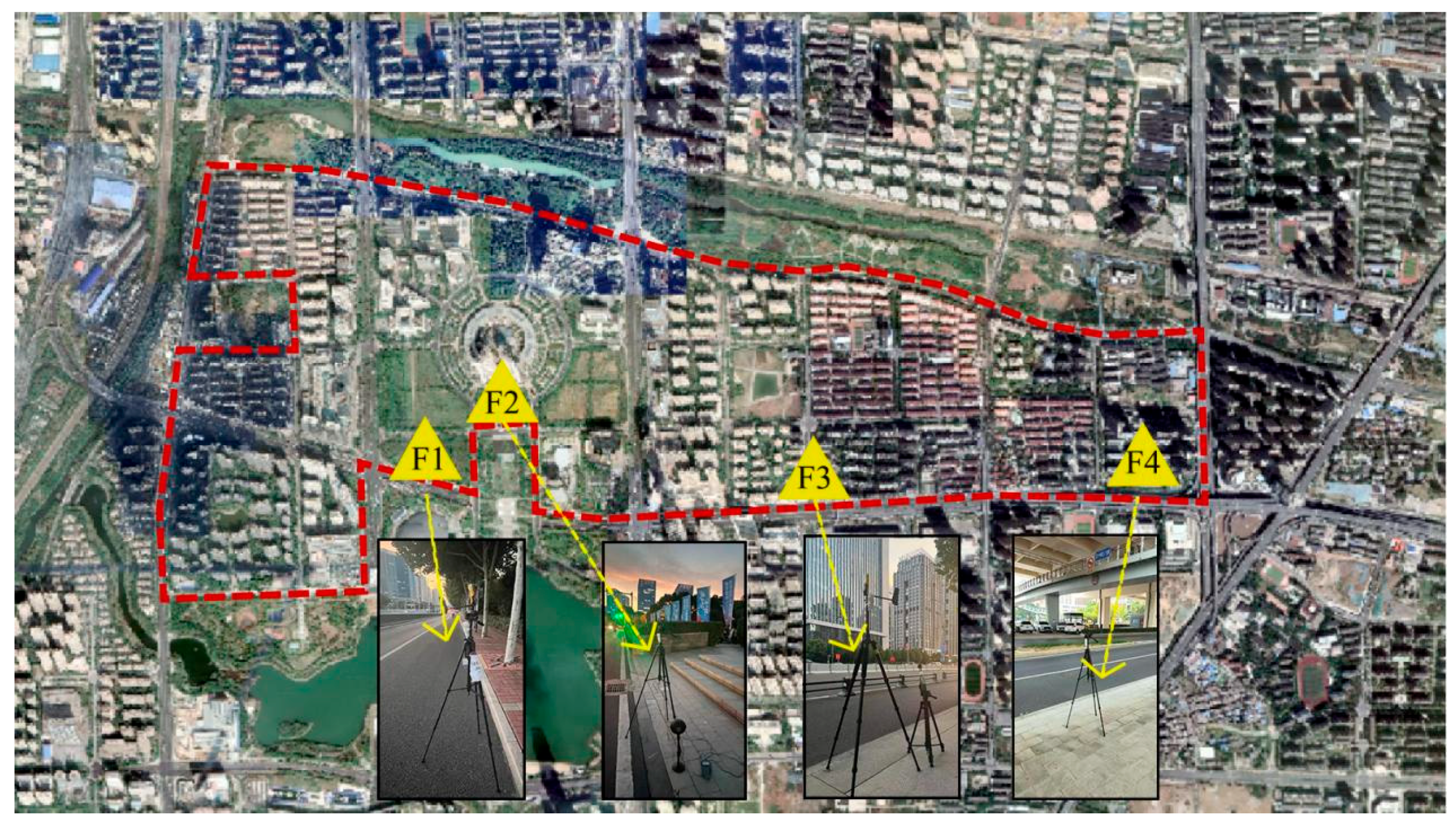
2.1. Study Area

Hefei is situated in eastern China, within the Jianghuai Plain, characterized by an undulating landscape and minimal geographical variation. The subtropical humid monsoon climate is characterized by chilly winters and hot summers. In recent years, Hefei has experienced significant social and economic development, transitioning from a “ring city” to a “lake” configuration, resulting in an expansion of the urban built-up area. The city has been constructed on an increasingly expansive scale, transitioning from “lakefront” to “embrace the lake”. The rise in population density distribution, along with the nature of urban surface coverage and building design, has led to alterations that contribute to the complexity of spatial diversity [47]. The vicinity of Swan Lake in Hefei, a representative region of the city, was chosen as the study area to encompass a diverse array of built environment types, as illustrated in Figure 1. The study area encompasses multifunctional zones, including residential districts, commercial centers, entertainment venues, and urban parks, primarily featuring a mix of medium-to-high-rise and low-rise structures with diverse architectural designs, thereby facilitating a comprehensive sample of local climate zones (LCZs). The LCZ scheme has been utilized to assess the spatial morphology of the case area [48]. This paper employs a neighborhood-based LCZ classification method [49] to categorize the urban neighborhood units within the case area into various LCZ types, thereby illustrating the heterogeneity of urban morphology, as depicted in Figure 1.

2.2. Research Methods

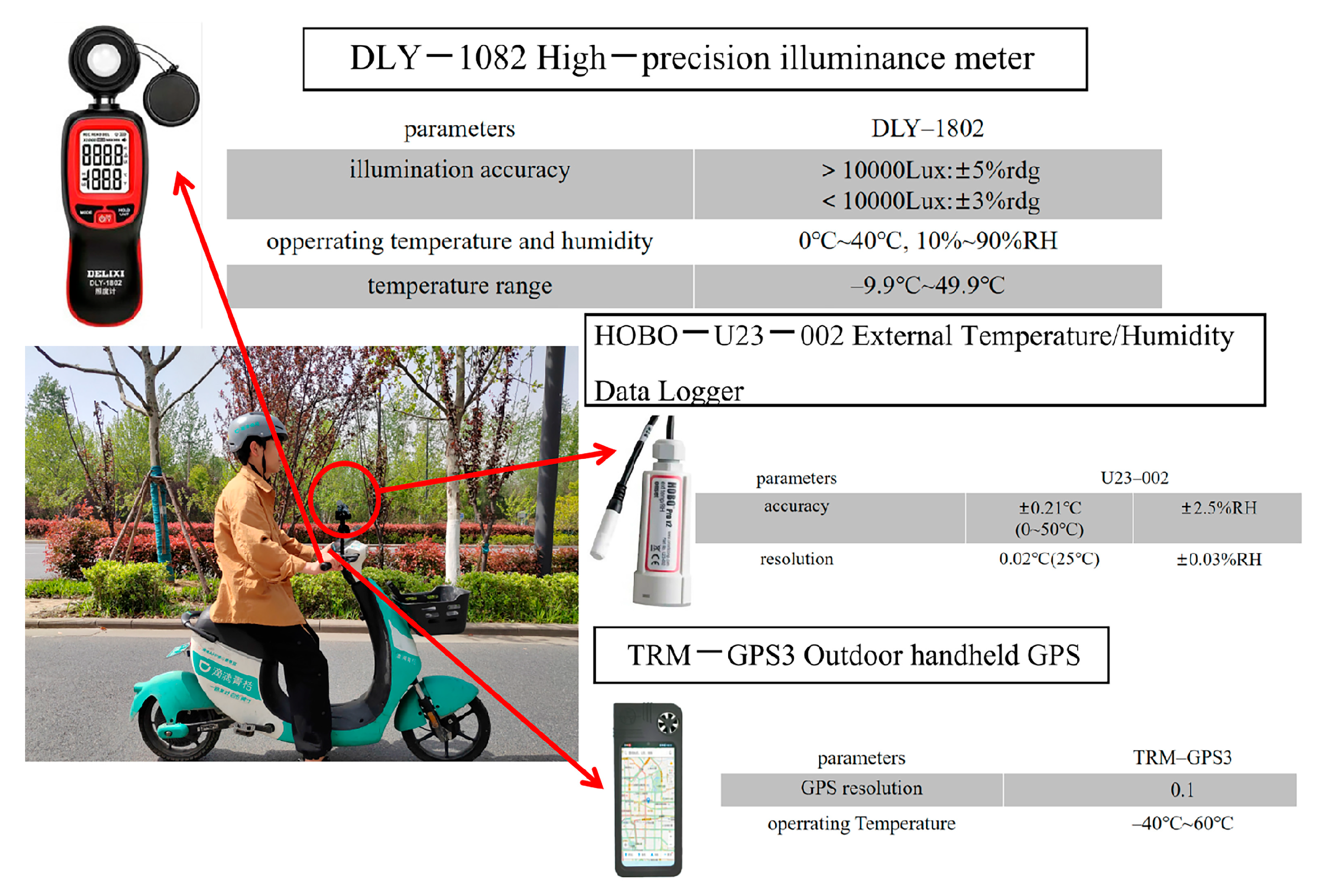
2.2.1. Mobile Measurement Program

This study involved the creation of a closed mobile route encompassing forty-one mobile test locations surrounding Swan Lake in Hefei, utilizing six concurrently running fixed weather stations and four validating weather stations, as seen in Figure 1. The research location is situated near the water, with negligible traffic congestion. The mobile test route included a total length of 10 km, encompassing 41 mobile measurement locations with varying surroundings and configurations, from dispersed low-rise building zones to densely crowded urban centers. Six fixed weather stations (HOBO-U23-002), designated as FS01 through FS06, served as time-adjusted reference stations, while four validation weather stations, labeled VSO1 through VS04, were employed to assess the errors of the four temporal correction models. To address the various underlying surface conditions of the reference stations, the six station LCZ types—LCZ1, LCZ2, LCZ3, LCZ4, and LCZ8—along with the site environments of these four weather stations, are presented.

A mobile measurement was conducted using an e-bike equipped with a portable, radiation-shielded external temperature and humidity recorder (HOBO U23-002) and a GPS to identify the 41 test sites. The apparatus was fixed to the e-bike at a height of 1.5 m above the ground, as illustrated in Figure 2. Data from the air temperature and relative humidity logger, together with GPS, were recorded at one-minute intervals to assure the precision of each test site. An illuminance meter (DLX-1082) was employed to document the shading along the moving route, and it was calibrated using data from ArcGIS. Furthermore, the e-bikes maintained an average velocity of 20–30 km/h and primarily traversed slow lanes to approach the local thermal environment while minimizing exposure to thermal emissions from vehicular traffic.

The mobile polls were conducted on 18 August 2023; 18 November 2023; 23 January 2024; and 12 April 2024, with testing occurring at 9:00, 11:00, and 15:00, respectively. Initially, to guarantee the safety and comfort of the measures, it is essential to consider that rain may disrupt the efficacy of unsheltered mobile surveys conducted on an e-bike. Moreover, intense precipitation and damp circumstances can impair the GPS signal transmission and diminish the positional accuracy of mobile surveys, while the spatial attributes of the local thermal environment on rainy days may significantly differ from those on dry days. Thermal environment parameters were concurrently documented at stationary weather stations at one-minute intervals. Although mobile measurement has been recognized by many scholars for the study of thermal environments and the heat island effect in urban spaces, there is a very important problem in the application of mobile measurement, which is the heterogeneity of thermal environment parameters obtained by mobile testing methods in time and space. First, these mobile measurement data are recorded by the mobile equipment moment by moment during the observation along the route, and with the change in background meteorological parameters, the non-simultaneous data cannot be directly compared. Second, it is known from the literature that the formation of thermal environment parameters at different location points is usually affected by the urban spatial morphology and different types of underlying surface configurations, and the amount of changes in thermal environment parameters at different location points will be similarly changed by the thermal effects of the environment in which they are located. The routes of mobile tests usually pass through complex urban neighborhoods, which are greatly influenced by the surrounding dense buildings and traffic flow, etc. Therefore, with the changes of the underlying surface characteristics during the mobile observation process, the observation data obtained by the mobile tests are spatially heterogeneous, and the same cannot be directly compared and analyzed. From the above, it can be seen that although the mobile test method has the advantage of covering a large local area and diversified geographical conditions, the spatial and temporal heterogeneity of the test data makes the mobile test method itself have limitations in its application. Therefore, the problem of temporal heterogeneity of mobile measurements with temporal corrections is addressed in subsequent papers.

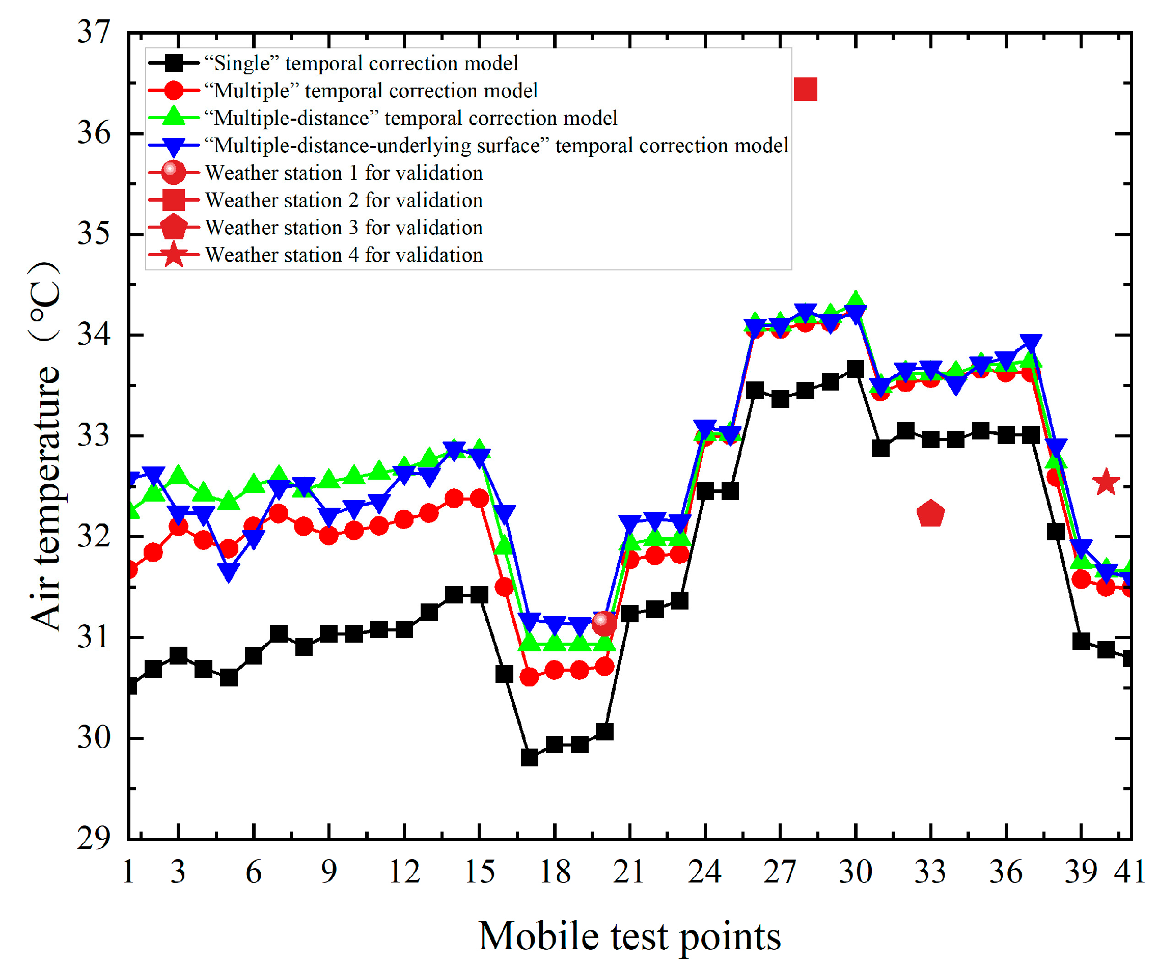
2.2.2. Introduction of the Classical Temporal Correction Model

The article contrasts four typical spatial and temporal correction models, which are as follows: the “Single” temporal correction model, the “Multiple” temporal correction model, the “Multiple-distance” temporal correction model, and the “Multiple-distance-underlying surface” temporal correction model. These models exhibit distinct attributes in temporal correction.

Table 1. Exposition of four distinct temporal correction models.

Models	Station Number	Calculation Formula
“Single” temporal correction model [50]	N = 1	$y_{j,tr}-y_{j,tj}=x_{j,tr}-x_{j,tj}$
“Multiple” temporal correction model [41]	N > 1	$y_{j,tr}-y_{j,tj}={\displaystyle \sum _{i=1}^N\left(x_{i,tr}-x_{i,tj}\right)}/N$
“Multiple-distance” temporal correction model [32]	N > 1	$y_{j,tr}-y_{j,tj}={\displaystyle \sum _{i=1}^N\left(x_{i,tr}-x_{x,tj}\right)}\ast l_{ij}{⠀}^{-2}/{{\displaystyle \sum _{\mathrm{i}=1}^N{l}_{ij}}}^{-2}$
“Multiple-distance-underlying surface” temporal correction model [43]	N > 1	$\begin{array}{l}{y}_{j,tr}-y_{j,tj}={\displaystyle \sum _{i=1}^N\left[k_{ij}\left(x_{i,tr}-x_{i,tj}\right)\right]}/N\\ k_{ij}=A\ast {\displaystyle \frac{p_j}{p_i}}+B\ast {\displaystyle \frac{l_{ij}}{l}}+c\end{array}$

Note. N: quantity of meteorological stations; y_j,tr: the thermal environment parameter at mobile test location j during the uniform reference moment tr; y_j,tj: the thermal environment parameter at mobile test location j at test time t_j; x_i,tr: the thermal environment parameter at fixed weather station i during the uniform reference moment tr; x_i,tj: the thermal environment parameter at fixed weather station i at test time t_j. l_ij: the precise distance between fixed weather station i and mobile location j; l denotes the overall length of the mobile route. k_ij: the influence of underlying surface conditions and the distance between a fixed weather station and mobile site j on the correlation coefficient; l: the total length of the mobile route; Pi: the underlying surface characteristic parameter of station i; P_j: the underlying surface characteristic parameter of mobile location j; A: the coefficient of the subsurface characteristic term; B: the coefficient of the spatial distance scale term; C: the coefficient of the constant term.

presents the specific spatial and temporal correction models.

This paper also compares the accuracy of different temporal correction models by means of mean absolute error (MAE) and root mean square error (RMSE), which are calculated using Equations (1) and (2), respectively.

$$MAE={\sum }_{y=1}^4\left|v_{ya}-v_{yc}\right|/4$$

(1)

$$RMSE=\sqrt{{\displaystyle \frac{{\sum }_{y=1}^4{\left(v_{ya}-v_{yc}\right)}^2}{4}}}$$

(2)

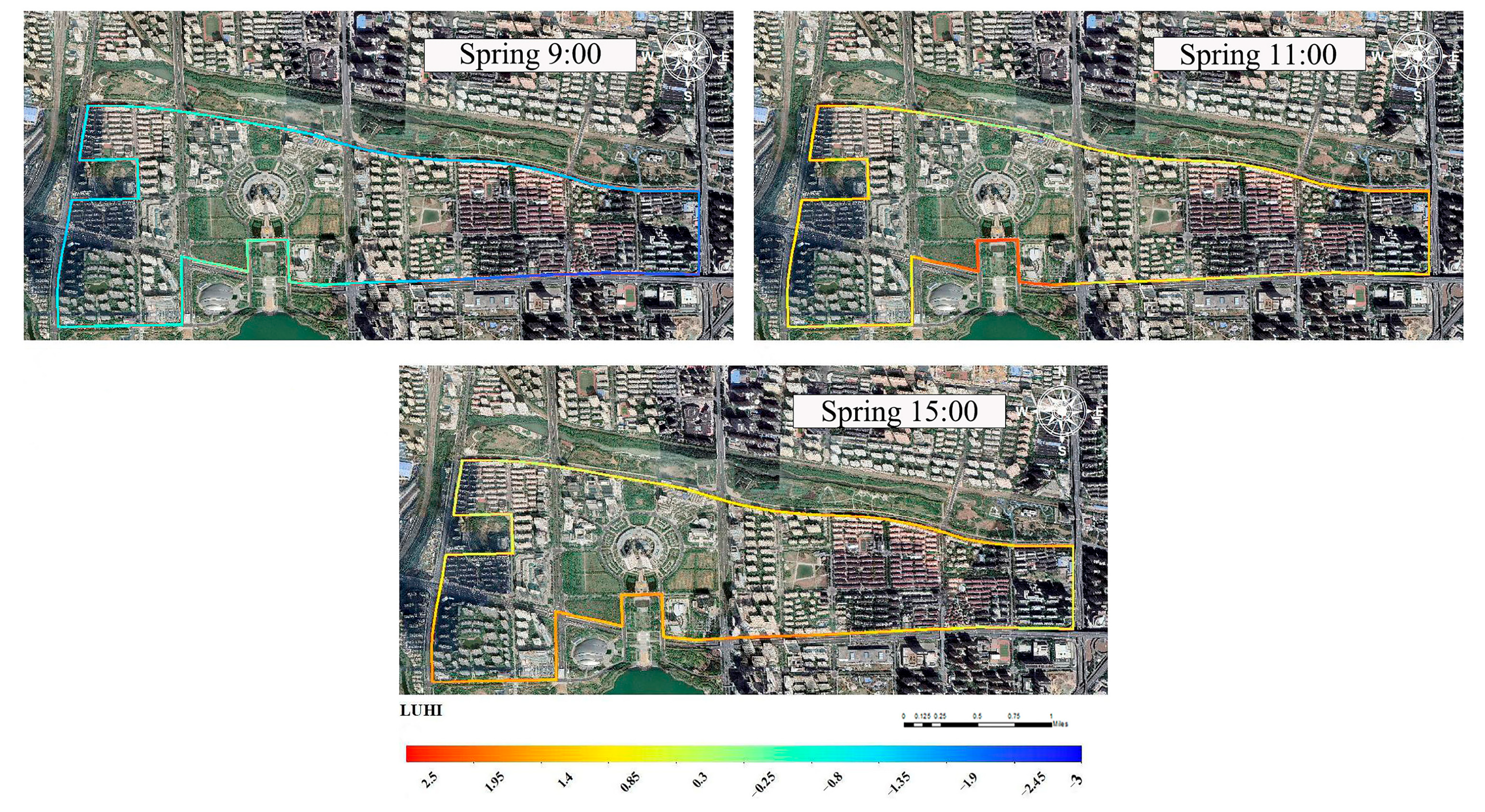
2.2.3. Local Heat Island Intensity

Mobile measurements are implemented inside the study region to acquire air temperature data at several test points along the mobile route during different seasons, which are crucial for quantitatively analyzing the thermal environment disparities across the mobile test stations. This paper delineates the disparities in the thermal environments of mobile test sites through localized heat island intensity (LUHI) values [51,52], and it compares the adjusted air temperatures at these test sites along mobile routes to those recorded at reference meteorological stations in suburban areas, thereby facilitating the precise calculation of LUHI values at multiple temporal points for the mobile test sites; furthermore, the suburb location is chosen to be Hefei Xinqiao Airport. The precise computation of the local heat island intensity value (LUHI) is shown in Equation (3). LUHII is the local heat island intensity at location point i at the observation time t; Tit represents the temperature at location point i at the observation time t; and T_st indicates the temperature of the suburb at the observation time t.

$$LUHI=T_{it}-T_{st}$$

(3)

2.2.4. ArcGIS Spatial Interpolation Method

This work employed the spatial interpolation approach to derive a continuous spatial field of the measured parameters [53], utilizing recorded measurement point data to anticipate data for unknown regions. The Kriging method is utilized in spatial interpolation as a regression procedure for spatial modeling and the prediction of stochastic processes, relying on covariance function and variational function models. In contrast to other spatial interpolation techniques, the Kriging method emphasizes the impact of spatially extensive autocorrelation of regional variables on the weights. Therefore, we used the “Geostatistical Analyst” module of ArcGIS 10.8 software for spatial interpolation of LUHI, so as to obtain the temporal distribution of LUHI along the whole moving route.

3. Research Results

3.1. Comparison of Error Results of Four Temporal Correction Models

The validation outcomes of Ta were articulated through the mean absolute error (MAE) and root mean square error (RMSE) by comparing the reference and adjusted temperatures (Ta) to each spatiotemporally corrected model, as illustrated in Figure 3. The formulas for computing the MAE and RMSE are delineated as Equation (2) and Equation (3), respectively.

In this context, v_ya and v_yc represent the temperature recorded by the validated weather station at the specific moment and the temperature at that moment following the adjustment of location points along the mobile measurement route, respectively; y signifies the identifier for the validated weather stations; and the adjusted air temperature values derived from various temporal correction models are illustrated in Figure 3. Despite the small error of the “Multiple-distance-underlying surface” temporal correction model, the large difference in the temperature between validation point two and validation three and the corresponding measurement points on the moving route is due to the fact that the area where validation point two is located is a plaza, which is not surrounded by any building or environment for shade, while validation point three is surrounded by a high-rise building, which is able to provide shade, hence the large difference in the temperature between the two validation points.

The accuracies of several temporal correction models are evaluated based on the MAE and RMSE error values, as presented in

Table 2. Temperature correction error results based on four temporal correction models.

Models	Air Temperature
	MAE (°C)	RMSE (°C)
“Single” temporal correction model	1.615	1.829
“Multiple” temporal correction model	1.282	1.454
“Multiple-distance” temporal correction model	1.236	1.410
“Multiple-distance-underlying surface” temporal correction model	1.144	1.387

. The “Multiple-distance-underlying surface” temporal correction model exhibits the lowest MAE value for Ta, succeeded by the “Single” temporal correction model, the “Multiple” temporal correction model, and the “Multiple-distance” temporal correction model. The MAE value of the “Multiple-distance-underlying surface” temporal correction model is approximately 1.144 °C, but the MAE values of the other temporal correction models exceed 1.2 °C. Additionally, the RMSE value of the “Multiple-distance-underlying surface” model is 1.387 °C. Furthermore, the RMSE value of Ta for the remaining three spatial and temporal correction models exceeds that of the “Multiple-distance-underlying surface” temporal correction model. Consequently, the “Multiple-distance-underlying surface” temporal correction model exhibits superior accuracy compared to the alternative models. The error results imply a significant fluctuation in the MAE and RMSE values of the “Single” temporal correction model compared to the other three correction models. The analysis indicates that the underlying surface properties exert the most substantial influence on the correlations among the various places, as informed by the four models’ influences.

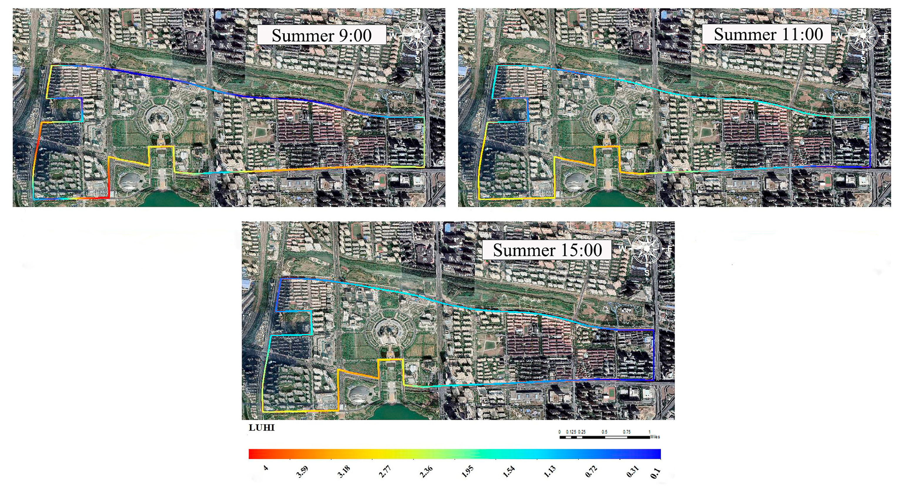
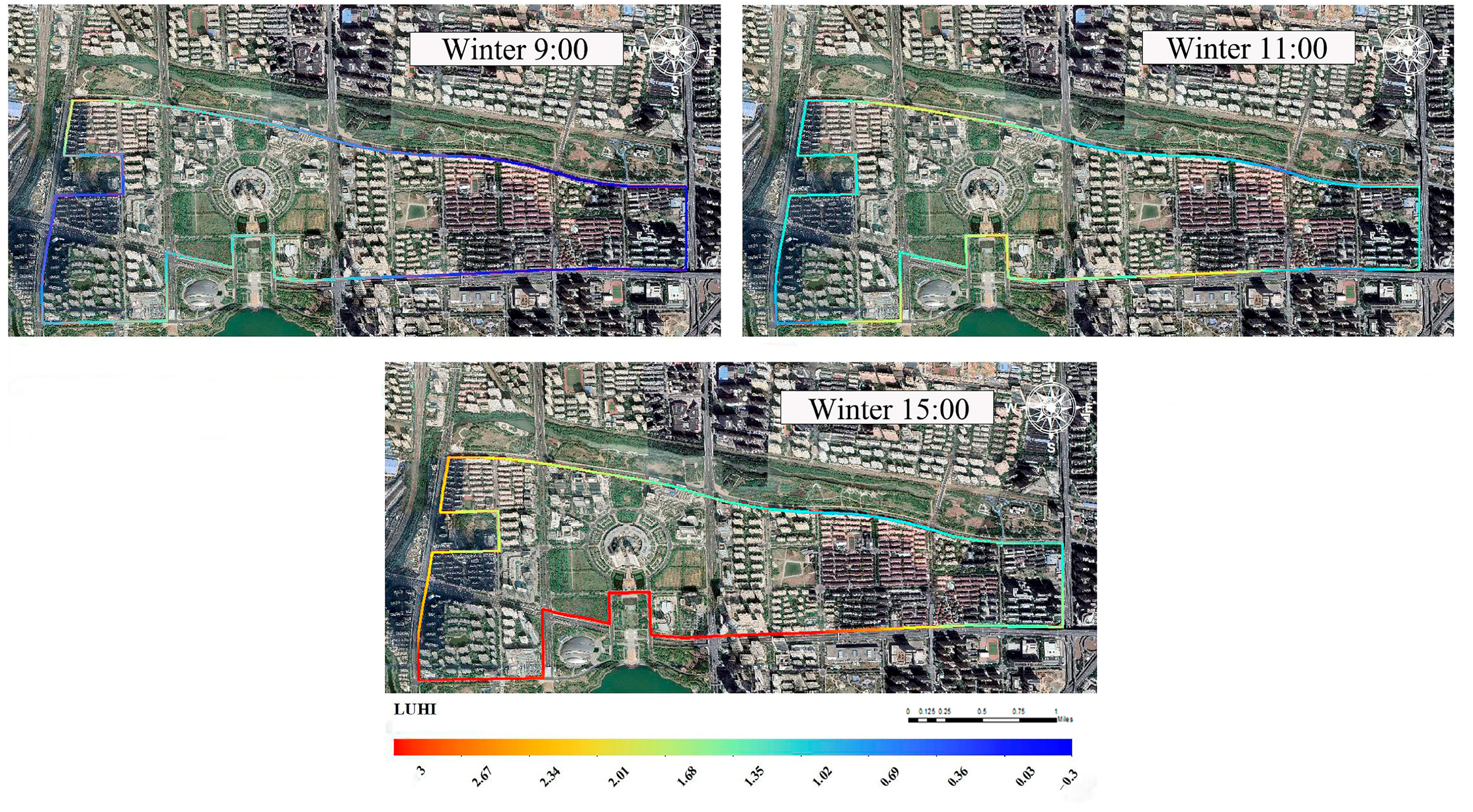
3.2. Distribution of Heat Island Intensity Along the Movement Route

The precise distribution of heat island intensity along the moving routes was examined in relation to the four zones depicted in Figure 4. In the comprehensive analysis of Figure 5, the LUHI values in the Hefei Swan Lake research region throughout various moments of the spring testing period predominantly ranged from −3 °C to 2.5 °C along the mobile measurement routes. The spatial distribution of LUHI values across various moments on mobile routes exhibits considerable spatial disparities; nevertheless, the variability of the heat island intensity distribution over the entire routes in spring is not substantial. Zone 2 primarily consists of a dense high-rise building complex, with LUHI values in this area progressively increasing over time, while the heat island intensity at 9:00 is minimal. The maximum LUHI value in this region attains 1.95 °C post 11:00. Figure 6 illustrates the spread of local heat island intensity along the summer mobile measuring route. The disparity in heat island intensity distribution along the summer mobile route is more pronounced than in spring; however, Zone 3 maintains a higher LUHI value. Despite the presence of green space in this area, it is significantly influenced by solar radiation due to its open nature, resulting in an elevated LUHI value. Zone 1 comprises the People’s Park, where the abundant greenery significantly mitigates heat island intensity, particularly during the summer months. Zone 2 and Zone 4 are both high-rise residential districts; however, a notable disparity exists in the distribution of heat island intensity. This variation arises because the mobile route in Zone 2 is obscured by a viaduct, resulting in a lower LUHI value for this route due to the combined shading effects of the building and the viaduct, while the LUHI value for the surrounding area remains elevated. The LUHI values are diminished, attaining 0.1 °C, approaching the LUHI values of the park adjacent to Zone 1. In contrast, the shading along the mobility route in Zone 3 is inconsistent, resulting in elevated LUHI values, indicative of greater heat island intensity in that region. Figure 7 depicts the distribution of local heat island intensities along the mobile measurement route in autumn, revealing a distribution that closely resembles that of spring and exhibits minimal variability in heat island intensities. Figure 8 illustrates the spread of heat islands during the winter measuring period, revealing significant variations in heat island strength at different times. The LUHI value of Zone 1 remains low, exhibiting the “cold island effect”. Zones 3 and 4 demonstrate a more pronounced heat island effect, with the maximum LUHI value reaching 3 °C. Zone 2’s LUHI value, influenced by shading, also attains 3 °C. Zone 2 maintains a reduced LUHI, which is attributable to its shade impact.

Analysis of the annual distribution of heat island intensity reveals significant variability during spring and autumn movement routes, with LUHI values spanning from −3 to 2.5 °C. In contrast, the variability during summer movement routes is more pronounced, exhibiting LUHI values from 0.1 to 4 °C. Despite Zone 3 having a greater proportion of green space, its LUHI value is elevated, contradicting the common belief that green space mitigates the heat island effect [54]. Additionally, the LUHI value of Zone 2 is markedly higher than that of the other regions at 15:00. Throughout the year, the same high-rise buildings encircle Zone 3; however, the LUHI value is elevated in comparison to Zone 4. Since Block 3 is surrounded by a square area, the temperature in the square area is very high and the hot air from the square flows into the area of the moving route, causing the moving route to show higher LUHI values. Consequently, we hypothesized that the shading effect influences the distribution of heat island intensity along the mobile routes. Four representative measurement points were subsequently selected for a more in-depth analysis of the underlying causes of this phenomenon. Refer to Section 3.3.

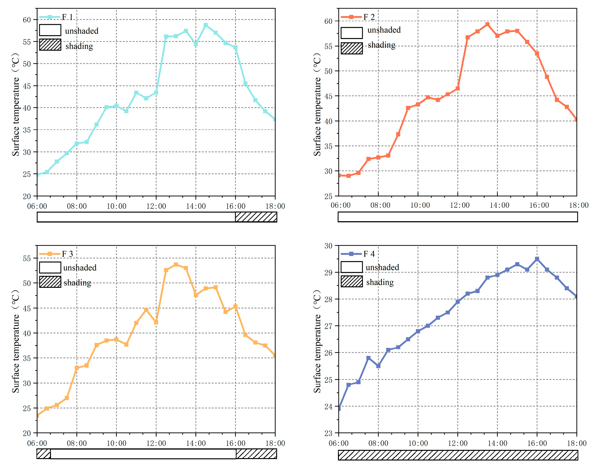
3.3. Impact of Shading on UHI on Mobile Route

This section analyzes the impact of shade on the thermal environment of the slow lane by selecting representative measurement stations throughout the route, with field observations conducted on 28 September 2024 from 6 a.m. to 6 p.m. The positions of the four designated measuring spots are illustrated in Figure 9. Fixed weather stations (HOBO-U23-002) were installed at an elevation of approximately 1.5 m above ground level, designated F1 to F4, and surface temperatures were taken and documented at 30 min intervals. The Ts was measured and documented every 30 min using an infrared thermal imager (UTi160s) to capture images of the area surrounding the weather stations, with infrared images taken bi-hourly. Additionally, a black sphere recorder (Taiwan Hengxin AZ8758) was positioned at measurement points two and three to record the temperature of the black sphere every 5 min. The instrumentation locations are illustrated in Figure 9, with the black spheres having resolutions of 0.1 °C, 1.5 °F, and 0.5 °C. The black spheres were positioned roughly 1 m above the ground. The black sphere recorder has a resolution of 0.1 °C and an accuracy of ±3 °C under outdoor conditions, while the infrared thermal imager (UTi160s) has a resolution of 0.1 °C and an accuracy of ±2 °C. The black sphere recorder (Taiwan Hengxin AZ8758) was positioned at Station 2 and Station 3 to monitor the black sphere temperature at 5 min intervals.

The influence of shading variations on the thermal conditions of the mobile route was meticulously examined by collecting data on shading alterations, surface temperatures, meteorological parameters, and thermograms at the sites of the four stationary meteorological measurement stations. Figure 10 illustrated the surface temperature and shadow variation data collected from the four designated sites. The figure illustrated the variations in air temperature (Ta) at four measurement locations at various times during the day. According to the trend of surface temperature variations, the observation period was segmented into the following three intervals: period 1 (06:00–12:00), period 2 (11:00–16:00), and period 3 (16:00–18:00). The air temperature (Ta) trend at several measurement places exhibited similarity throughout the observation period, consistently rising throughout time periods 1 and 2, peaking at approximately 14:00, and subsequently declining, as illustrated in Figure 11.

The disparities in Ta among F1, F2, and F3 are minimal; however, the discrepancies in Ta between F4 and the other three sites are significant, with a maximum average difference in Ta ranging from 3 to 5 °C at various periods during the day, as shown in Figure 11. In comparing the average hourly Ta, only F4 exhibits a substantial difference from F1, F2, and F3, with F4 regularly recording the lowest Ta, averaging 1.7–2.1 °C lower than F1, F2, and F3. Among all measurement stations, F3 recorded the highest Ta during time period 1; however, this diminished markedly after 14:00. Conversely, F2 exhibited the highest Ta in time period 2, while F3 again had the highest Ta in time period 3. Moreover, F4 exhibited the shade structure of a viaduct and reported a somewhat higher Ta compared to the other three measurement points over the three period intervals. The maximum disparity in Ta readings between shaded and unshaded Ta at measurement points FI and F3 was approximately 11.9 °C, while F2 emerged as the hottest location at the onset of time period 2 due to the escalation of solar radiation. The mean surface temperature variations are significantly diverse throughout the observation period, arranged in increasing order, as follows: F4 < F3 < F1 < F2, with F2’s mean surface temperature being 17.4 °C greater than that of F4.

Figure 12 illustrates that the shading circumstances influenced both the magnitude and distribution of the average Ts and air temperature at various measurement locations. At 8:00 am, a distinct contrast in the coloration of the images adjacent to F1 and F3 is evident, alongside a notable disparity in the Ts of the slow lane, which is attributable to the shading effects of the trees. The Ts of F1 registers at 24.1 °C under shade and 28.3 °C in unshaded conditions, while F3 exhibits a Ts of 27.5 °C when shaded and 29.4 °C when unshaded. Currently, F4 was influenced by the viaduct’s shade, resulting in a Ts of 20.8 °C, but F2, situated in an unobstructed area, experienced a Ts of 29.8 °C during the testing period. At 14:00, when the sun’s elevation angle rises, the canopy gap widens, allowing more direct sunlight to reach the ground, resulting in an increased distribution of high-temperature zones. The thermal distributions of F1, F2, and F3 illustrate the influence of shading on the surface temperature. Specifically, beneath the complete shading of the viaduct, the Ts of the road at F4 is lower than that at the other three measurement points, registering at 23.7 °C. Conversely, F2 emerges as a high-temperature zone, exhibiting a Ts of 45.6 °C, followed by F1 and F3. F1 experiences a surface temperature of 49.6 °C without shading and 45.4 °C with shading, while F3 records a Ts of 40.4 °C without shading and 37.5 °C with shading. The temperature changes depicted on the maps indicate that shading substantially influences temperature.

Further analysis of the effects of summer and winter shading strategies on the thermal environment revealed that shading variability on the summer and winter movement routes was reflected in the type of trees. Deciduous broadleaf trees are planted along the street on the slow lane in Hefei, and the trees planted along the moving lines in the study area were deciduous broadleaf trees alternating with evergreen trees, sycamore, and magnolia respectively. Therefore, in the summer months, greater shading was provided to the slow lane due to the alternation of the two types of trees. In winter, the sycamore trees, although deciduous, still provided shading due to their large crowns, alternating with magnolias.

3.4. Analysis of the Factors Influencing the Hot Loop of a Slow-Moving Road

3.4.1. Permeable Underlying Surface (PSF)

Initially, the impact of the permeable underlying surface on the air temperature along the mobile route is examined, with the results of correlating air temperature to the percentage of permeable underlying surface illustrated in Figure 13. This indicates a positive correlation between the permeable underlying surface and air temperature, suggesting that the permeable underlying surface does not substantially enhance the air temperature. Furthermore, the permeable underlying surfaces at the mobile measuring points consist entirely of trees interspersed with shrubs, and the varying percentages of underlay surrounding the measuring point are noted. The permeable underlying surface primarily consists of grass and plants, and it does not effectively facilitate cooling in areas F1, F2, and F3, surrounding the underlay.

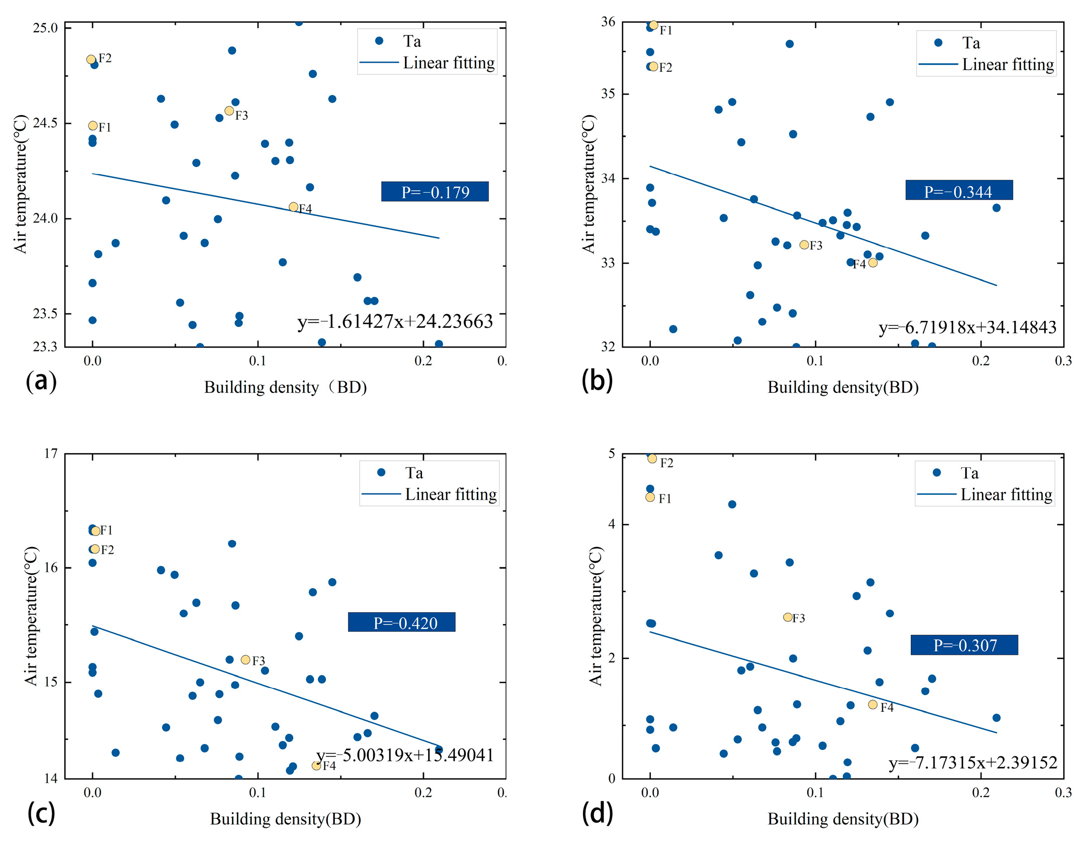
3.4.2. Building Density (BD)

Concerning the influence of building density on air temperature along the transit route, as illustrated in Figure 14, there exists a negative correlation between building density and air temperature. This suggests that increased building density may enhance the thermal environment of the slow-moving road to a certain degree. Furthermore, Figure 14b indicates that, during summer, measurement points F3 and F4 fall below the fitted line, while measurement points F1 and F2 are positioned above it. Notably, the locations of measurement points F3 and F4 correspond to an area characterized by high-density, high-rise buildings. The resultant building shade can enhance the thermal conditions of the slow lane.

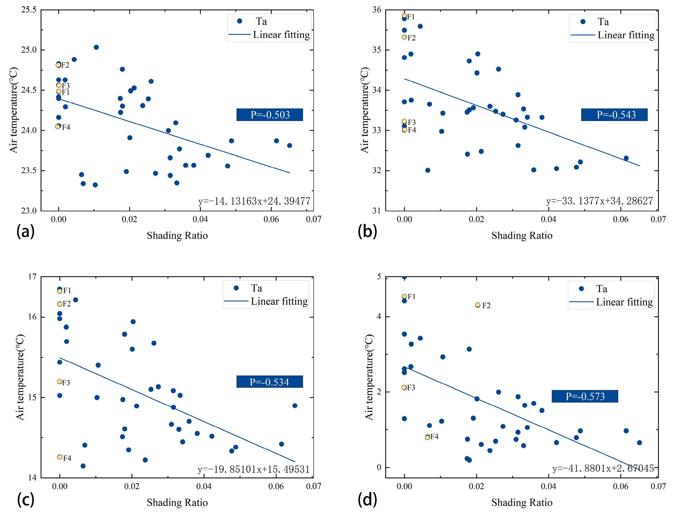
3.4.3. Shading Ratio (SR)

Figure 15 illustrates the correlation analysis between air temperature variation and shading rate at pedestrian height throughout the year. The shading rate is derived from satellite imagery processed in ArcGIS, specifically through edge-tracing techniques. The processing results indicate the percentage of shaded area within a 100 m radius from the measurement points along the mobile route. It is evident that the correlation between shading rate and air temperature along the mobile route is both stronger and negatively correlated; an increase in shading rate contributes to the mitigation of the thermal environment at pedestrian height. Fixed measurement points F1 and F2 consistently lie above the fitted line in the figure, indicating that the cooling effect in the absence of shading is less pronounced.

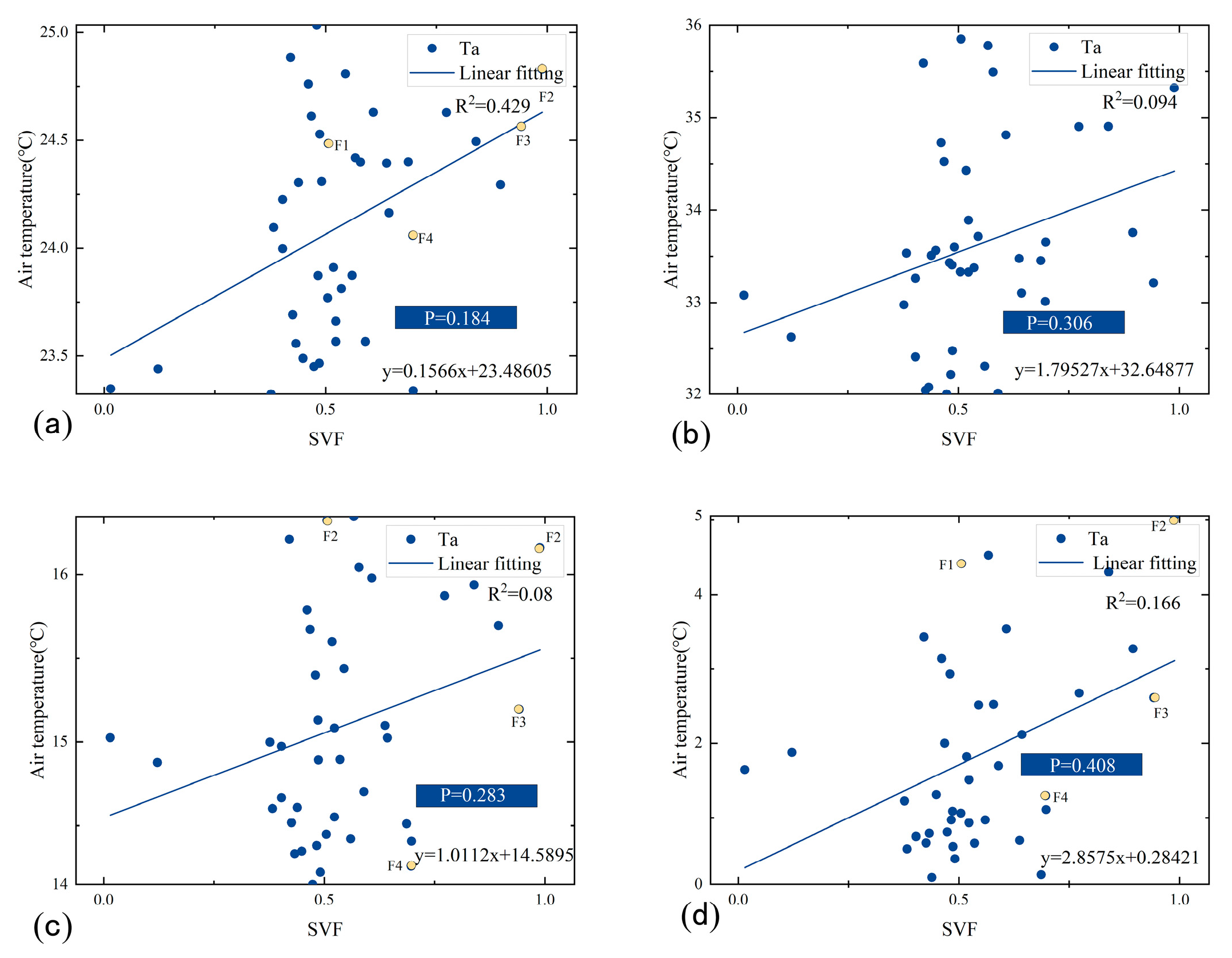
3.4.4. Sky View Factor (SVF)

Figure 16 illustrates the correlation analysis between temperature variations throughout the year and the sky view factor. The sky view factor was calculated by processing fisheye photographs with Rayman software. The processing results show the degree of shading of the buildings and environment around different measurement points on the moving route. It is obvious that the correlation between SVF and air temperature at the measurement points on the mobile route is stronger and positive; it indicates that the shading of buildings and trees on the mobile route can significantly reduce the air temperature.

3.4.5. Multivariate Fitting Analysis

The annual air temperature data, together with the associated PSF, BD, and SR percentages, underwent a multiple linear regression analysis, resulting in distinct fitting equations for each season, namely Equations (4) to (7) for spring, summer, autumn, and winter, respectively. The r-squared values of 0.372, 0.517, 0.533, and 0.458, respectively, demonstrated a positive association between the ground surface (PSF) and temperature and a negative correlation between the building density (BD) and shading ratio (SR). To further analyze the impact of thermal environment characteristics on thermal weight, the standardized coefficients of each parameter were compared.

$$y=0.562\ast PSF+-1.238BD+-11.285\ast SR+0.697\ast SVF+23.901$$

(4)

$$y=2.101\ast PSF+-5.807\ast BD+-31.595\ast SR+0.480\ast SVF+33.864$$

(5)

$$y=1.105\ast PSF+-4.513\ast BD+-19.178\ast SR+0.1925\ast SVF+15.424$$

(6)

$$y=0.929\ast PSF+-6.370\ast BD+-36.045\ast SR+1.333\ast SVF+2.078$$

(7)

Table 3. The standardized coefficients for the terms PSF and SR in Equation (4) to Equation (6), respectively.

Terms	Standardized Coefficients for Terms in Equation (4)	Standardized Coefficients for Terms in Equation (5)	Standardized Coefficients for Terms in Equation (6)	Standardized Coefficients for Terms in Equation (7)
PSF	0.193	0.332	0.286	0.123
BD	−0.138	−0.297	−0.379	−0.272
SR	−0.402	−0.517	−0.516	−0.493
SVF	0.259	0.082	0.054	0.190

illustrates that the standardized coefficients of the SR term much exceed those of the PSF and BD terms, signifying that the influence of shade on air temperature is more pronounced than that of ground and building density. Consequently, the influence of shadowing must be considered in the relationship between mobile points and stationary meteorological stations when implementing spatial and temporal adjustments in mobile measurements.

4. Discussion

4.1. Comprehensive Analysis of Different Underlying Surface Parameters Affecting Slow Lane Thermal Environment

In this study, multiple linear regression analysis was used to reveal the main influencing factors affecting the thermal environment of urban slow lanes, mainly analyzing the mechanisms of permeable underlying surface, building density, shading, and SVF factors on the thermal environment.

Firstly, it was found that in high-density cities, the increase of a permeable underlying surface can mitigate the heat island effect, which is consistent with the findings of Chen, RN [55]. They noted that green spaces, water bodies, and permeable brick pavements could mitigate the urban heat island effect. Our analysis of the effect of permeable understory on the urban thermal environment is inadequate, and the analysis of the results of the study shows that the increase in permeable understory is not able to mitigate the LUHI, so it is necessary to classify the different types of vegetation to analyze their impact on the thermal environment. Secondly, building density also affects changes in the thermal environment. Building density has a warming effect, leading to an increase in the heat island effect within the city [56]; however, in actual high-density cities, building density does not determine the urban thermal environment, but is also affected by other factors [57]. Finally, the shading ratio can significantly reduce air temperature and improve the urban heat island effect in areas with higher SVF values. Higher SVF values provide a more open view of the sky, which affects the thermal environment in localized areas [58]. However, there is no distinction made between the different vegetation types and the constituent shading of buildings to analyze their different shading effects.

4.2. Urban Thermal Environment Optimization Recommendations

In this study, we propose a comprehensive optimization plan for improving the thermal environment of urban pedestrian slow lanes by addressing the results of the effects of different underlying surface parameters on the thermal environment of urban slow lanes.

Firstly, given the finding that shading significantly reduces temperature, it is recommended to increase the density of tree planting in the public space of the studied slow lanes. High-shade-species, such as deciduous trees, should be planted in areas with high heat island intensity, especially in areas with little shading. These trees will provide adequate shading at critical times, reduce air temperatures, and increase humidity through transpiration. In addition, taking into account the difference in the distribution of heat island intensity between summer and winter, and the fact that trees lose their leaves in winter, the trees planted in the slow lanes should alternate between evergreen trees and deciduous trees, so that the ability to ensure the effect of shade in summer can also improve the comfort of pedestrians in winter. A well-designed tree-planting scheme can reduce the surrounding area’s temperature by an additional 1.5 °C throughout the year. In downtown Los Angeles, the positive cooling effects of trees during periods of hot weather significantly outweigh the negative impacts during colder periods. By strategically placing trees to maximize shading and considering seasonal variations, cities like Los Angeles can effectively enhance thermal comfort and mitigate the urban heat island effect [59]. The proposed tree-planting strategies offer practical guidance for urban planners and are broadly applicable, providing valuable insights for cities beyond Los Angeles. Secondly, optimizing the layout of buildings is an important regulatory measure. By adjusting the height and location of the building, it will be able to provide more shading at noon and afternoon, effectively reducing direct sunlight. Utilizing the shading effect of buildings can create cooler air for slow lanes and improve the urban heat island effect. Proper use of SVF is also key to optimizing the thermal environment of the slow lanes. By controlling the height and width of tree canopies to maintain adequate sky openings, slow lanes can benefit from good natural lighting and air circulation while avoiding excessive shading that blocks the view of the sky. Finally, improving infrastructure and amenities along slow lanes is also an important optimization measure.

4.3. Limitations of the Study

In line with previous studies, it can be said that this study investigates the air temperature effects of the pedestrian-level on slow lanes at a micro scale using mobile measurements, and our results show that there are differences in the applicability of different temporal correction models, which makes it particularly important to select a temporal correction model that is applicable to one’s study area. Secondly, there are differences in the effects of different underlying surface parameters on the thermal environment of the slow lanes, and the shading factor is particularly important to create a more comfortable spatial environment for the slow lane space and to bring comfort to pedestrians travelling in summer. Our study has several limitations. Firstly, the current acquisition of the underlying surface parameters is not detailed enough to distinguish the vegetation types from the permeable underlying surface. In addition, the underlying surface parameters can be further expanded to analyze the mechanism of the influence of the underlying surface parameters on the thermal environment [60]. Secondly, among the effects of shading on the thermal environment, the effects of grass and trees on the thermal environment are different, and there are also differences in the effects of shading composed of buildings and shading composed of vegetation on the thermal environment, so we will further differentiate the effects of shading composed of vegetation and buildings on the thermal environment, and analyze the effects of shading on the thermal environment in depth. We can use the Rhinoceros software and the Grasshopper3 platform to further analyze and study LUHI [61]. We will follow-up on this research with a study on the urban spatial morphology and underlying surface parameters to deeply analyze the specific mechanism of their influence on the thermal environment by using machine learning models, as well as unmanned aerial vehicles.

5. Conclusions

This research examines the urban thermal environment by utilizing the mobile measurement method. Initially, the precision of various temporal correction models is evaluated, followed by the application of temporal correction to the thermal environment parameters derived from mobile measurements. This is integrated with the spatial interpolation technique of ArcGIS to visualize the distribution of heat island intensity along mobile routes, facilitating an analysis of the variations in heat island intensity distribution at different times of the year and the impact of the underlying surface on the thermal environment of these routes. Additionally, we analyzed the impact of shading on the thermal environment. The results show that the “Multiple-distance-underlying surface” temporal correction model exhibits the lowest MAE value for Ta, around 1.144 °C, with an RMSE value of 1.387 °C. The MAER and MSE of Ta for the other three temporal correction models exceed 1.2 °C, surpassing those of the “Multiple-distance-underlying surface” temporal correction model. Consequently, the “Multiple-distance-underlying surface” temporal correction model has superior accuracy compared to alternative models.

Upon comparing the distribution characteristics of LUHI throughout the year, it is evident that the intensity of the heat island along the mobile route varies temporally and spatially. Notably, there is no significant disparity in heat island intensity distribution along the mobile route during spring and autumn, while the most pronounced difference occurs in the summer, followed by winter. The LUHI ranges from 0.1 to 4 in summer and from −0.3 to 3 in winter, with findings indicating that LUHI values in high-rise building areas exhibit both elevated and diminished heat island intensities.

The analysis of measurements at four representative points reveals that shading influences the variations in the thermal environment along the travel route. The air temperatures at F4 exhibit a greater disparity compared to the other three measuring points. A comparison of their average hourly air temperatures indicates that the temperature values at the point located beneath the viaduct are markedly distinct from those at the other three locations, with a maximum average difference in Ta ranging from 3 to 5 °C across various time intervals, and an overall average that is 1.7 to 2.0 °C lower than that of the remaining three measuring points. The sequence of mean Ts across the tests, in ascending order, was F4 < F3 < F1 < F2. The mean surface temperature at F2 was approximately 17.4 °C greater than that at F4, as F4 was obscured by the viaduct, which diminishes shortwave radiation, reaching the ground more effectively than the tree shading at F1.

The analysis of the thermal environmental influences on Ta revealed that the standardized coefficients for shading were considerably greater than those for permeable ground and building density. This indicates that the shading factor exerted a more substantial impact on Ta variations along the mobile measurement route than the permeable underlying surface. The influence of shade on temperature changes was most pronounced in winter, followed by summer. The standardized coefficient for winter shade is −0.572, and for summer shade it is −0.551.

This study investigated the effects of different underlying surface parameters on the thermal environment of urban slow lanes based on a mobile measurement method. The accuracy of different temporal correction models for mobile measurements is evaluated. By comparing the distribution of heat island intensity along the mobile route in different seasons, it can be found that summer and winter exhibit the most significant disparities, with heat island intensity values fluctuating between 0.1 and 4 in summer and between −0.3 and 3 in winter.

In addition, the provision of shading is crucial in the urban planning process. This human-to-human focus paves the way for a more systematic improvement of the urban heat island effect. Therefore, the government should encourage the development of horticulture and green buildings to improve the localized heat island intensity of slow lanes, mitigate the urban heat island effect, and continuously improve the living environment for residents.

References

1. Xie, Q.; Sun, Q. Monitoring thermal environment deterioration and its dynamic response to urban expansion in Wuhan, China. Urban Clim. 2021, 39, 100932. [Google Scholar] [CrossRef]
2. Wang, M.; Lu, H.; Chen, B.; Sun, W.; Yang, G. Fine-Scale Analysis of the Long-Term Urban Thermal Environment in Shanghai Using Google Earth Engine. Remote Sens. 2023, 15, 3732. [Google Scholar] [CrossRef]
3. Kim, S.W.; Brown, R.D. Urban heat island (UHI) intensity and magnitude estimations: A systematic literature review. Sci. Total Environ. 2021, 779, 146389. [Google Scholar] [CrossRef]
4. Ding, N.; Zhang, Y.; Wang, Y.; Chen, L.; Qin, K.; Yang, X. Effect of landscape pattern of urban surface evapotranspiration on land surface temperature. Urban Clim. 2023, 49, 101540. [Google Scholar] [CrossRef]
5. Guzman, L.A.; Arellana, J.; Castro, W.F. Desirable streets for pedestrians: Using a street-level index to assess walkability. Transp. Res. Part D 2022, 111, 103462. [Google Scholar] [CrossRef]
6. Hong, S.; Luo, Y.; Zhu, Y.; Huang, C.; Li, Y.; Sun, C. Childhood respiratory diseases related to indoor and outdoor extreme thermal environment (air temperature) in Shanghai, China. Indoor Built Environ. 2024, 33, 341–358. [Google Scholar] [CrossRef]
7. Cao, X.; Tang, B.; Zou, X.; He, L. Analysis on the cooling effect of a heat-reflective coating for asphalt pavement. Road Mater. Pavement Des. 2015, 16, 716–726. [Google Scholar] [CrossRef]
8. Cleland, S.E.; Steinhardt, W.; Neas, L.M.; West, J.J.; Rappold, A.G. Urban heat island impacts on heat-related cardiovascular morbidity: A time series analysis of older adults in US metropolitan areas. Environ. Int. 2023, 178, 108005. [Google Scholar] [CrossRef]
9. Lee, M.; Kim, S.; Kim, H.; Hwang, S. Pedestrian visual satisfaction and dissatisfaction toward physical components of the walking environment based on types, characteristics, and combinations. Build. Environ. 2023, 244, 110776. [Google Scholar] [CrossRef]
10. Zhang, X.; Kasimu, A.; Liang, H.; Wei, B.; Aizizi, Y.; Zhao, Y.; Reheman, R. Construction of Urban Thermal Environment Network Based on Land Surface Temperature Downscaling and Local Climate Zones. Remote Sens. 2023, 15, 1129. [Google Scholar] [CrossRef]
11. Atri, M.; Nedae-Tousi, S.; Shahab, S.; Solgi, E. The Effects of Thermal-Spatial Behaviours of Land Covers on Urban Heat Islands in Semi-Arid Climates. Sustainability 2021, 13, 13824. [Google Scholar] [CrossRef]
12. Lu, Y.; Yue, W.; Liu, Y.; Huang, Y. Investigating the spatiotemporal non-stationary relationships between urban spatial form and land surface temperature: A case study of Wuhan, China. Sustain. Cities Soc. 2021, 72, 103070. [Google Scholar] [CrossRef]
13. Zhou, X.; Chen, H. Experimental Analysis of the Influence of Urban Morphological Indices on the Urban Thermal Environment of Zhengzhou, China. Atmosphere 2021, 12, 1058. [Google Scholar] [CrossRef]
14. Ibrahim, A.; Ali, H.; Abuhendi, F.; Jaradat, S. Thermal seasonal variation and occupants’ spatial behaviour in domestic spaces. Build. Res. Inf. 2019, 48, 364–378. [Google Scholar] [CrossRef]
15. Yang, J.; Nam, I.; Sohn, J.-R. The influence of seasonal characteristics in elderly thermal comfort in Korea. Energy Build. 2016, 128, 583–591. [Google Scholar] [CrossRef]
16. Yin, P.; Xie, J.; Ji, Y.; Liu, J.; Hou, Q.; Zhao, S.; Jing, P. Winter indoor thermal environment and heating demand of low-quality centrally heated houses in cold climates. Appl. Energy 2023, 331, 120480. [Google Scholar] [CrossRef]
17. Mallick, J. Evaluation of Seasonal Characteristics of Land Surface Temperature with NDVI and Population Density. Pol. J. Environ. Stud. 2021, 30, 3163–3180. [Google Scholar] [CrossRef]
18. Fang, Z.; Zhang, F.; Guo, Z.; Zheng, Z.; Feng, X. Investigation into the outdoor thermal comfort on different urban underlying surfaces. Urban Clim. 2024, 55, 101911. [Google Scholar] [CrossRef]
19. Cheela, V.R.S.; John, M.; Biswas, W.; Sarker, P. Combating Urban Heat Island Effect—A Review of Reflective Pavements and Tree Shading Strategies. Buildings 2021, 11, 93. [Google Scholar] [CrossRef]
20. Zou, Z.; Yan, C.; Yu, L.; Jiang, X.; Ding, J.; Qin, L.; Wang, B.; Qiu, G. Impacts of land use/ land cover types on interactions between urban heat island effects and heat waves. Build. Environ. 2021, 204, 108138. [Google Scholar] [CrossRef]
21. Rahman, M.A.; Dervishi, V.; Moser-Reischl, A.; Ludwig, F.; Pretzsch, H.; Rötzer, T.; Pauleit, S. Comparative analysis of shade and underlying surfaces on cooling effect. Urban For. Urban Green. 2021, 63, 127223. [Google Scholar] [CrossRef]
22. Shu, B.; Chang, H.T.; Chen, Y.X. Influence of the thermal environment of urban sidewalks under green shading from a human scale. All Earth 2024, 36, 127223. [Google Scholar] [CrossRef]
23. Kong, H.; Choi, N.; Park, S. Thermal environment analysis of landscape parameters of an urban park in summer—A case study in Suwon, Republic of Korea. Urban For. Urban Green. 2021, 65, 127377. [Google Scholar] [CrossRef]
24. Meili, N.; Acero, J.A.; Peleg, N.; Manoli, G.; Burlando, P.; Fatichi, S. Vegetation cover and plant-trait effects on outdoor thermal comfort in a tropical city. Build. Environ. 2021, 58, 107733. [Google Scholar] [CrossRef]
25. Meili, N.; Manoli, G.; Burlando, P.; Carmeliet, J.; Chow, W.T.; Coutts, A.M.; Roth, M.; Velasco, E.; Vivoni, E.R.; Fatichi, S. Tree effects on urban microclimate: Diurnal, seasonal, and climatic temperature differences explained by separating radiation, evapotranspiration, and roughness effects. Urban For. Urban Green. 2020, 58, 126970. [Google Scholar] [CrossRef]
26. Manley, G. On the frequency of snowfall in metropolitan England. Q. J. R. Meteorol. Soc. 1958, 84, 70–72. [Google Scholar] [CrossRef]
27. Basu, R.; Ostro, B.D. A multicounty analysis identifying the populations vulnerable to mortality associated with high ambient temperature in California. Am. J. Epidemiol. 2008, 168, 632–637. [Google Scholar] [CrossRef]
28. Manoli, G.; Fatichi, S.; Schläpfer, M.; Yu, K.; Crowther, T.W.; Meili, N.; Burlando, P.; Katul, G.G.; Bou-Zeid, E. Magnitude of urban heat islands largely explained by climate and population. Nature 2019, 573, 55. [Google Scholar] [CrossRef]
29. Mohite, S.; Surawar, M. Impact of urban street geometry on outdoor pedestrian thermal comfort during heatwave in Nagpur city. Sustain. Cities Soc. 2024, 108, 105450. [Google Scholar] [CrossRef]
30. Pan, Y.; Li, S.; Tang, X. Investigation of Bus Shelters and Their Thermal Environment in Hot–Humid Areas—A Case Study in Guangzhou. Buildings 2024, 14, 2377. [Google Scholar] [CrossRef]
31. Kim, E.J.; Kim, H. Walking-based mobile measurement: Examining its reliability for spatial thermal characteristics in urban environments. Urban Clim. 2024, 58, 102154. [Google Scholar] [CrossRef]
32. Jiang, L.; Zhao, H.; Cao, B.; He, W.; Yun, Z.; Cheng, C. A UAV Thermal Imaging Format Conversion System and Its Application in Mosaic Surface Microthermal Environment Analysis. Sensors 2024, 24, 6267. [Google Scholar] [CrossRef] [PubMed]
33. Parison, S.; Hendel, M.; Royon, L. A statistical method for quantifying the field effects of urban heat island mitigation techniques. Urban Clim. 2020, 33, 100651. [Google Scholar] [CrossRef]
34. Parison, S.; Chaumont, M.; Kounkou-Arnaud, R.; Long, F.; Bernik, A.; Da Silva, M.; Hendel, M. The effects of greening a parking lot as a heat mitigation strategy on outdoor thermal stress using fixed and mobile measurements: Case-study project “tertiary forest”. Sustain. Cities Soc. 2023, 98, 104818. [Google Scholar] [CrossRef]
35. Ye, X.; Ren, H.; Wang, P.; Duan, Y.; Zhu, J. Urban LST Retrieval From the Ultrahigh Spatial Resolution Remote Sensing Data. IEEE Geosci. Remote Sens. Lett. 2024, 21, 7000305. [Google Scholar] [CrossRef]
36. Costanzini, S.; Despini, F.; Beltrami, L.; Fabbi, S.; Muscio, A.; Teggi, S. Identification of SUHI in Urban Areas by Remote Sensing Data and Mitigation Hypothesis through Solar Reflective Materials. Atmosphere 2022, 13, 70. [Google Scholar] [CrossRef]
37. Luo, T.; He, Q.; Wang, W.; Fan, X. Response of summer Land surface temperature of small and medium-sized cities to their neighboring urban spatial morphology. Build. Environ. 2024, 250, 111198. [Google Scholar] [CrossRef]
38. Schnell, I.; Cohen, P.; Mandelmilch, M.; Potchter, O. Portable-trackable methodologies for measuring personal and place exposure to nuisances in urban environments: Towards a people oriented paradigm. Comput. Environ. Urban Syst. 2021, 86, 101589. [Google Scholar] [CrossRef]
39. Pigliautile, I.; D’eramo, S.; Pisello, A.L. Intra-urban microclimate mapping for citizens’ wellbeing: Novel wearable sensing techniques and automatized data-processing. J. Clean. Prod. 2021, 279, 123748. [Google Scholar] [CrossRef]
40. Sundborg, A. Climatlogical studies in Uppsala with special regard to the temperature conditions in the urban area. Georaphica 1951, 22. [Google Scholar]
41. Masashi, M.; Minako, N.; Masaki, N.; Masatoshi, N. Study on temperature distribution of an urbanized area using a vehicle with mobile measurement system. J. Environ. Eng. 2009, 74, 1179–1185. [Google Scholar]
42. Leconte, F.; Bouyer, J.; Claverie, R.; Pétrissans, M. Using Local Climate Zone scheme for UHI assessment: Evaluation of the method using mobile measurements. Build. Environ. 2015, 83, 39–49. [Google Scholar] [CrossRef]
43. Liu, L.; Liu, J.; Lin, Y. Spatial-temporal Analysis of the Urban Heat Island of a Subtropical City by Using Mobile Measurement. Procedia Eng. 2016, 169, 55–63. [Google Scholar] [CrossRef]
44. Cao, C.; Yang, Y.; Lu, Y.; Schultze, N.; Gu, P.; Zhou, Q.; Xu, J.; Lee, X. Performance Evaluation of a Smart Mobile Air Temperature and Humidity Sensor for Characterizing Intracity Thermal Environment. J. Atmos. Ocean. Technol. 2020, 37, 1891–1905. [Google Scholar] [CrossRef]
45. Emery, J.; Pohl, B.; Crétat, J.; Richard, Y.; Pergaud, J.; Rega, M.; Zito, S.; Dudek, J.; Vairet, T.; Joly, D.; et al. How local climate zones influence urban air temperature: Measurements by bicycle in Dijon, France. Urban Clim. 2021, 40, 101017. [Google Scholar] [CrossRef]
46. Chàfer, M.; Tan, C.L.; Cureau, R.J.; Hien, W.N.; Pisello, A.L.; Cabeza, L.F. Mobile measurements of microclimatic variables through the central area of Singapore: An analysis from the pedestrian perspective. Sustain. Cities Soc. 2022, 83, 103986. [Google Scholar] [CrossRef]
47. Shimazaki, Y.; Aoki, M.; Nitta, J.; Okajima, H.; Yoshida, A. Experimental Determination of Pedestrian Thermal Comfort on Water-Retaining Pavement for UHI Adaptation Strategy. Atmosphere 2021, 12, 127. [Google Scholar] [CrossRef]
48. May, S.; Oliphant, A.J. Characteristics of the Park Cool Island in Golden Gate Park, San Francisco. Theor. Appl. Climatol. 2023, 151, 1269–1282. [Google Scholar] [CrossRef]
49. Jin, L.; Pan, X.; Liu, L.; Liu, L.; Liu, J.; Gao, Y. Block-based local climate zone approach to urban climate maps using the UDC model. Build. Environ. 2020, 186, 107334. [Google Scholar] [CrossRef]
50. Fung, W.Y.; Lam, K.S.; Nichol, J.; Wong, M.S. Derivation of Nighttime Urban Air Temperatures Using a Satellite Thermal Image. J. Appl. Meteorol. Climatol. 2009, 48, 863–872. [Google Scholar] [CrossRef]
51. Zhou, Y.; Luo, Y.; Yi, X.; Lun, F.; Hu, Q.; Huang, N.; Wen, G.; Zhou, H.; Hu, X. Exploring the influence of local urban heat features on park cooling effects: Insights from Chinese cities. Build. Environ. 2024, 262, 111782. [Google Scholar] [CrossRef]
52. Liu, L.; Lin, Y.; Wang, D.; Liu, J. Dynamic Spatial-temporal Evaluations of Urban Heat Islands and Thermal Comfort of a Complex Urban District Using an Urban Canopy Model. J. Asian Archit. Build. Eng. 2016, 15, 627–634. [Google Scholar] [CrossRef]
53. Yu, Z.; Song, Y.; Song, D.; Liu, Y. Spatial interpolation-based analysis method targeting visualization of the indoor thermal environment. Build. Environ. 2020, 188, 107484. [Google Scholar] [CrossRef]
54. Gong, Y.; Li, X.; Liu, H.; Li, Y. The Spatial Pattern and Mechanism of Thermal Environment in Urban Blocks from the Perspective of Green Space Fractal. Buildings 2023, 13, 574. [Google Scholar] [CrossRef]
55. Chen, R.; You, X. Reduction of urban heat island and associated greenhouse gas emissions. Mitig. Adapt. Strateg. Glob. Chang. 2020, 25, 689–711. [Google Scholar] [CrossRef]
56. Chen, X.; Wang, Z.; Bao, Y.; Luo, Q.; Wei, W. Combined impacts of buildings and urban remnant mountains on thermal environment in multi-mountainous city. Sustain. Cities Soc. 2022, 87, 104247. [Google Scholar] [CrossRef]
57. Yang, J.; Shi, B.; Xia, G.; Xue, Q.; Cao, S.-J. Impacts of Urban Form on Thermal Environment Near the Surface Region at Pedestrian Height: A Case Study Based on High-Density Built-Up Areas of Nanjing City in China. Sustainability 2020, 87, 1737. [Google Scholar] [CrossRef]
58. Wang, R.; Liu, R.; Chen, Q.; Cheng, Q.; Du, M. Effects of Sky View Factor on Thermal Environment in Different Local Climate Zoning Building Scenarios—A Case Study of Beijing, China. Buildings 2023, 13, 1882. [Google Scholar] [CrossRef]
59. Zhu, Y.; Kensek, K.M. Mitigating the Urban Heat Island Effect: The Thermal Performance of Shade-Tree Planting in Downtown Los Angeles. Sustainability 2024, 16, 8768. [Google Scholar] [CrossRef]
60. Elmarakby, E.; Khalifa, M.; Elshater, A.; Afifi, S. Tailored methods for mapping urban heat islands in Greater Cairo Region. Ain Shams Eng. J. 2022, 13, 101545. [Google Scholar] [CrossRef]
61. Elshater, A.; Abusaada, H.; Alfiky, A.; El-Bardisy, N.; Elmarakby, E.; Grant, S. Workers’ Satisfaction vis-à-vis Environmental and Socio-Morphological Aspects for Sustainability and Decent Work. Sustainability 2022, 14, 1699. [Google Scholar] [CrossRef]
Figure 1. Mobile measurement route and local climate zone (LCZ) distribution, along with the mobile measurement program (1 to 6, depicting the vicinity of permanent weather stations FS01-FS06).
Buildings 15 00388 g001
Figure 2. Mobile measurement tools and equipment.
Buildings 15 00388 g002
Figure 3. Comparison of correction outcomes from various temporal correction models.
Buildings 15 00388 g003
Figure 4. Four zones on the mobile measurement route.
Buildings 15 00388 g004
Figure 5. Distribution of LUHI values of mobile measurement route in the spring.
Buildings 15 00388 g005
Figure 6. Distribution of LUHI values of mobile measurement route in the summer.
Buildings 15 00388 g006
Figure 7. Distribution of LUHI values of mobile measurement route in the autumn.
Buildings 15 00388 g007
Figure 8. Distribution of LUHI values of mobile measurement route in the winter.
Buildings 15 00388 g008
Figure 9. Location of the four fixed weather stations.
Buildings 15 00388 g009
Figure 10. Distribution of surface temperature and shade at the four fixed sites.
Buildings 15 00388 g010
Figure 11. Average air temperature at four fixed measurement points.
Buildings 15 00388 g011
Figure 12. Thermal images of four measurement points taken at different times of the year.
Buildings 15 00388 g012aBuildings 15 00388 g012b
Figure 13. Correlation analysis between PSF and Ta ((a) for spring, (b) for summer, (c) for autumn, (d) for winter).
Buildings 15 00388 g013
Figure 14. Correlation analysis between BD and Ta ((a) for spring, (b) for summer, (c) for autumn, (d) for winter).
Buildings 15 00388 g014
Figure 15. Correlation analysis between shading ratio and Ta ((a) for spring, (b) for summer, (c) for autumn, (d) for winter).
Buildings 15 00388 g015
Figure 16. Correlation analysis between sky view factor and Ta ((a) for spring, (b) for summer, (c) for autumn, (d) for winter).
Buildings 15 00388 g016