Prediction of Compressive Strength of Carbon Nanotube Reinforced Concrete Based on Multi-Dimensional Database

Abstract

The incorporation of carbon nanotubes (CNTs) enhances the mechanical properties of cement-based materials by inhibiting micro-crack propagation. Machine learning provides an efficient approach for predicting the compressive strength of CNT-reinforced concrete, yet existing studies often lack important features and rely on less adaptive models. To address these issues, a multi-dimensional database (429 experimental data points) covering 11 factors (including cement mix ratio, CNT morphology, and dispersion process) was constructed. A hierarchical model verification and optimization was conducted: traditional regression models (Multiple Linear Regression, Multiple Polynomial Regression (MPR), Multivariate Adaptive Regression Splines), mainstream model (Support Vector Regression (SVR)), and ensemble learning models (Random Forest, eXtreme Gradient Boosting (XGB), Light Gradient Boosting Machine optimized by Particle Swarm Optimization (PSO)/Bayesian Optimization (BO)) are trained, compared, and evaluated. MPR performs best (test set R² = 0.856) among traditional regression models, while SVR (test set R² = 0.824) is less accurate. The highest accuracy in ensemble models is achieved by the PSO-optimized XGB model, with R² = 0.910 (test set). PSO outperforms BO in optimization precision, while BO is much more efficient. Water–cement ratio, age, and sand–cement ratio are the primary influencing factors for strength. Among CNT parameters, the inner diameter has greater impact than the length and outer diameter. Optimal CNT parameters are CNT–cement mass ratio 0.1–0.3%, inner diameter ≥ 7.132 nm, and length 1–15 μm. Surfactant polycarboxylate can increase strength, while OH⁻ functional groups can decrease it. These findings, integrated into the high-precision PSO-XGB model, provide a powerful tool for optimizing the mix design of CNT-reinforced concrete, accelerating its development and application in the industry.

1. Introduction

As one of the most principal construction materials, conventional concrete is a brittle material and is susceptible to cracking. To enhance the mechanical properties and durability of concrete, fiber-reinforced concrete was developed. The incorporation of fibers such as steel, glass, and polymer can effectively restrain the development of cracks at both micro- and macro-scales, thereby improving the toughness and strength [1,2,3,4,5,6]. However, conventional fibers exhibit a limited ability to inhibit nano-scale crack initiation and propagation. The development of micro-cracks can lead to a reduction in concrete strength [7]. To address this issue, the use of nanomaterials has been explored to improve the mechanical properties of concrete [8].

As a typical nanomaterial, carbon nanotubes (CNTs) possess excellent mechanical properties [9,10,11] and the advantage of low density. The incorporation of CNTs can control nano-scale micro-cracks within cement-based materials and thus exert a positive influence on the mechanical properties of cementitious composites [7]. However, the full potential of CNTs is often hindered by their tendency to agglomerate due to strong van der Waals forces [12]. Achieving uniform dispersion is therefore a critical challenge. Various techniques, such as pre-dispersion in water using surfactants or surface functionalization, have been developed to address this issue and improve the interaction between CNTs and the cement matrix [13].

The impact of CNTs on concrete strength has been studied extensively. Kumar et al. [14] investigated the effect of multi-walled carbon nanotubes (MWCNTs) on the strength of Portland cement mortar and found that the compressive and split tensile strengths of the composite reached their peaks when the MWCNT mass fraction was 0.5%, while the strength decreased when the content exceeded this value. Chaipanich et al. [15] revealed that a 0.5% CNT mass fraction optimized the flexural strength of mortar with silica fume. Syed et al. [16] showed that a 0.05% addition of MWCNTs increased the split tensile strength by 20.58% and the flexural strength by 26.29%. Xu et al. [17] found that 0.1% and 0.2% MWCNT contents increased the flexural strength of cement mortar by 30% and 40%, respectively. Wang [18] confirmed that CNTs significantly enhanced the flexural toughness index of Portland cement mortar, and that MWCNT incorporation improved pore size uniformity and reduced porosity. The 28-day test data indicated that the maximum fracture energy of the mortar reached 312.16 N/m, and its toughness increased by 47.1% (reaching 2.56) at 0.1% MWCNT content.

Based on the aforementioned research findings, it can be concluded that the enhancement of concrete strength by CNT incorporation is significant, with the influencing factors identified as CNT dispersion, mass fraction, and type. However, most existing experimental studies have focused on a single factor, often neglecting the synergistic effects among these variables. This highlights the need for a systematic and integrated analysis of their combined impact.

Concrete is an inherently complex system composed of various components, such as cementitious materials, aggregates, fibers, and admixtures, which are randomly distributed [19,20,21,22]. This heterogeneity makes it challenging to accurately predict its mechanical properties, especially its compressive strength [23,24,25]. While numerical simulations can predict concrete behavior, they are often hampered by the complexity, nonlinearity, and randomness of the interaction mechanisms between the components and the microstructure [26,27,28]. The prediction becomes even more intricate for CNT-enhanced concrete, where additives like nanofibers and surfactants are introduced. Factors such as CNT content, surfactant type, surface functionalization, and dispersion methods all influence the compressive strength. In recent years, machine learning (ML) has emerged as a promising alternative. Compared to traditional approaches, a distinct advantage of ML is that it can learn directly from data without being constrained by the underlying physical mechanisms and thus can provide more accurate predictions [29,30,31].

In predicting the mechanical properties of CNT-reinforced cement composites, researchers have predominantly focused on the accuracy of ML models. Decision Tree (DT) and Random Forest (RF) algorithms were employed by Nazar et al. [32] to estimate the compressive strength of nanomaterial-modified concrete, with the RF model showing superior performance and accuracy. Similarly, Jiao et al. [33] compared mainstream models (e.g., DT, Multi-Layer Perceptron Neural Network, Supported Vector Machine (SVM)) with ensemble methods (e.g., Bagging, Boosting), revealing that ensemble models significantly outperform standalone algorithms in error reduction and predictive capability.

Beyond model performance, other studies have delved into the influence of material characteristics. Huang et al. [34] noted that ML models exhibited stronger generalization for compressive strength prediction than traditional response surface methods. Their analysis identified CNT length as a key factor for compressive strength, while curing temperature had the most significant impact on flexural strength. Adel et al. [35] concluded that XGBoost achieved the highest reliability in predicting compressive and flexural strength compared to RF and AdaBoost. Their analysis further revealed a positive correlation between curing age and compressive strength, whereas the water–cement ratio, CNT content, and CNT diameter showed significant negative correlations. Other research has confirmed the significant impact of specimen size on 28-day compressive strength [36]. Yang et al. [37] utilized Gene Expression Programming (GEP) and Random Forest Approximation models, where the GEP model excelled in deriving empirical equations. The SHAP analysis identified the curing time, cement type, and water–cement ratio as the most influential factors. Li et al. [38] used SHAP to confirm that CNT content and diameter significantly affect compressive strength and identified the optimal parameters as a length of 20 μm, diameter of 25 nm, and content of up to 0.1%. However, it is noteworthy that the conclusions on key influencing factors are not consistent across these studies, which suggests potential systematic differences in their underlying datasets, feature selection, and modeling approaches.

Previous studies on ML models of the compressive strength of CNT-reinforced cementitious materials have significant discrepancies in feature selection, modeling algorithm adoption, and data volume. Basic parameters, including curing days and cement dosage, were selected by Jiao et al. [33] with 282 data points. Similarly, features such as the curing time and water–cement ratio were focused on by Yang et al. [37] with 282 data points. Huang [34] incorporated microscopic features like CNT morphology (outer diameter, length) and functional groups with a dataset of 114 points. Li et al. [39] used parameters, including curing time and cement content, based on 282 data points. Furthermore, Nazar et al. [32] selected features such as fine aggregate and cement content with 255 data points, while Adel [35] incorporated features like the water–cement ratio and CNT type based on 276 compressive and 261 tensile strength data points. Li et al. [38] involved features related to CNT dispersion with 149 and 107 data points for cement mortar and concrete, respectively. Manna [40] focused on parameters such as the cement dosage and water–cement ratio with 295 data points. Features related to the specimen size effect were considered by Yang et al. [36] with 151 data points.

A synthesis of the aforementioned studies reveals that while ML offers an effective approach for predicting the performance of CNT-reinforced concrete, existing research suffers from significant limitations. (1) Limited dataset size and incomplete feature dimensions: The feature sets adopted in different studies vary significantly, and the sample sizes are generally limited, typically ranging from 100 to 300 data points. The datasets for most predictive models do not adequately cover key control parameters that influence CNT dispersion performance. Specifically, they often lack features reflecting the dispersion process (e.g., sonication duration, type of dispersant, or surfactant) and specific surface chemical treatments. For instance, some studies [32,33,37] primarily focus on basic mix proportions and fundamental CNT parameters. Although other research incorporates some microscopic parameters [34,35], it still lacks consideration of specific dispersion process features. This deficiency makes it difficult for the models to accurately capture the complex influence of dispersion on strength. (2) Bias in model selection, with a tendency towards single model types or an insufficient number of comparative models: Current predictions predominantly rely on traditional ML algorithms and ensemble methods. However, there is a lack of comprehensive comparison and validation across these different model types, making it difficult to objectively evaluate the applicable scenarios and predictive value of each model.

To address the aforementioned limitations, this study establishes a predictive framework for the compressive strength of CNT-reinforced concrete based on a multi-dimensional database and multiple ML models. On the one hand, a comprehensive database was constructed with 429 experimental data points and with key CNT dispersion control parameters (e.g., sonication duration, surfactant type) and complete CNT morphological features (e.g., outer diameter, inner diameter, length). This multi-dimensional database covers 11 core influencing factors, including cementitious mix proportion parameters, CNT morphological features, dispersion process, interface modification, specimen geometry and size, and curing time. On the other hand, hyperparameter optimization and systematic validation of multiple ML models were implemented. Firstly, the performance of traditional regression models (Multiple Linear Regression (MLR), Multiple Polynomial Regression (MPR), Multivariate Adaptive Regression Splines (MARS)) was compared to identify the optimal model within this category. Secondly, Support Vector Regression (SVR), a mainstream classical model, was introduced as a reference to bridge traditional regression and ensemble models. Thirdly, ensemble learning models (Random Forest (RF), eXtreme Gradient Boosting (XGB), Light Gradient Boosting Machine (LGBM)) optimized with two hyperparameter tuning methods—Particle Swarm Optimization (PSO) and Bayesian Optimization (BO)—were compared to select the best-performing model in the ensemble category. Finally, a cross-type comparative validation was performed among the optimal traditional regression model, SVR, and the optimal ensemble learning model. This comprehensive evaluation assessed the predictive performance and applicable scenarios of different model types and identified the overall best prediction model. The methodological workflow of this study is summarized in Figure 1.

2. ML Models and Methods

2.1. Traditional Regression Model

Traditional regression models, as fundamental predictive methods in ML, are widely applied to model the relationship between a dependent variable and one or more independent variables. They are included here to establish a performance baseline, leverage their interpretability, and justify the need for more advanced algorithms. This study selects three classical regression models: MLR, MPR, and MARS.

2.1.1. Multiple Linear Regression

MLR fits data using a linear equation to model the relationship between a dependent variable and multiple independent variables, with the fundamental form presented in Equation (1):

$$y={\beta }_0+{\beta }_1{X}_1+{\beta }_2{X}_2+\cdots +{\beta }_p{X}_p+\epsilon ,$$

(1)

where $y$ is the dependent variable, and $X_1$, $X_2$, $\cdots$, $X_p$ are the independent variables. ${\beta }_0$ is the intercept term, and ${\beta }_1$, ${\beta }_2$, $\cdots$, ${\beta }_p$ are the regression coefficients, each representing the independent influence of its corresponding independent variable on the dependent variable. ε is the random error term of the model.

The regression coefficients are estimated using the Ordinary Least Squares (OLS) method by minimizing the Residual Sum of Squares (RSS), as shown in Equation (2):

$$RSS\left(\beta \right)={\sum }_{i=1}^N{{(y_i-(\beta }_0+{\sum }_{j=1}^p{X}_{i,j}·{\beta }_j\left)\right)}^2,$$

(2)

where $y_i$ is the observed value of the i-th sample, $X_{i,j}$ is the value of the j-th independent variable for the i-th sample, and $N$ is the total number of samples.

Key assumptions of MLR include linearity, error normality, independence, and homoscedasticity [41]. In practical applications, the simplicity and interpretability of MLR make it widely used.

2.1.2. Multiple Polynomial Regression

MPR is an extension of linear regression that captures non-linear relationships by introducing higher-order terms (e.g., quadratic, cubic) of the independent variables [42]. The MPR model can be expressed as Equation (3):

$$y={\beta }_0+{\beta }_{1}X+{\beta }_2{X}^2+\cdots +{\beta }_d{X}^d,$$

(3)

where $d$ is the degree of the polynomial, and ${\beta }_0$, ${\beta }_1$, ${\beta }_2$, $\cdots$, ${\beta }_d$ are the regression coefficients. The coefficients in MPR are calculated using the same method as in linear regression, optimized via OLS.

To prevent overfitting in the MPR model, this study employs Ridge Regression for regularization. Ridge Regression adds an L2 penalty term to the loss function [43], which is the sum of the squared model parameters (${\omega }_j$) multiplied by a penalty coefficient, α. This process shrinks coefficients to improve generalization. The loss function for Ridge Regression is shown in Equation (4):

$$min Loss{(y,\widehat{y})}_{ridge}={\sum }_{i=1}^N{(y_i-{\omega }_0-{\sum }_{j=1}^p{x}_{ij}{\omega }_j)}^2+\alpha {\sum }_{j=1}^p{{\omega }_j}^2,$$

(4)

where the choice of the polynomial degree (d) is crucial for the model’s performance. A degree that is too low may lead to underfitting, while a degree that is too high can cause overfitting. Therefore, the optimal degree is typically determined using methods such as cross-validation. According to the Weierstrass Approximation Theorem, any continuous function can be uniformly approximated by a polynomial function [44]. Due to its simple form, ease of interpretation, and computational efficiency, MPR is one of the most commonly used models.

2.1.3. Multivariate Adaptive Regression Splines

MARS is a non-parametric regression technique that models relationships using piecewise linear basis functions (BFs), whose number and parameters are automatically determined from the data [45]. The MARS model, $f\left(x\right)$, is a linear combination of BFs, as shown in Equation (5):

$$y=f\left(x\right)={\sum }_{m=1}^M{\beta }_m{\rho }_m\left(x\right),$$

(5)

where ${\rho }_m$ is a BF, which can be a piecewise linear function or an interaction BF formed by multiplying existing terms.

MARS simplifies complex datasets by fitting piecewise linear segments known as splines, which are smoothly connected to form the overall model. The connection points of the splines are called knots, and their locations are determined through a search process to minimize the Sum of Squared Errors (SSE). The MARS model is developed in forward and backward stages, using a spline expansion form as shown in Equation (5) to determine the approximate number and location of knots [46]. Equation (6) shows the form of a BF, where $t$ is the knot (a constant) and $x$ is the variable:

$$h\left(x-t\right)=\left\{\begin{array}{c}\left(x-t\right),x>t\\ 0,x\le t\end{array}\right..$$

(6)

The development of a MARS model involves two stages. (1) Forward pass: A large set of BFs is generated by searching for single-variable knots and examining interactions between variables. This process continues until a maximum number of BFs is reached, resulting in a complex and likely overfitted model. (2) Backward pass: The model’s performance is evaluated using the Generalized Cross-Validation (GCV) criterion. BFs that contribute least to the model’s performance are pruned to select the optimal model. The mathematical expression for GCV is given in Equation (7) [47]:

$$GCV={\displaystyle \frac{\frac{1}{N}{\sum }_{i=1}^N{\left[y_i-f\left(x_i\right)\right]}^2}{{\left[1-\frac{C\left(B\right)}{N}\right]}^2}},$$

(7)

where N is the number of data points, and B is the number of BFs in the model. $C\left(B\right)$ is a complexity penalty that increases with the number of BFs, expressed as Equation (8):

$$C\left(B\right)=(B+1)+\lambda B,$$

(8)

where λ is a penalty coefficient for each BF included in the model.

The advantage of MARS lies in its ability to automatically identify non-linear relationships and interaction effects between variables while avoiding strong assumptions about the underlying data distribution. This makes MARS particularly effective for handling complex datasets.

2.2. Support Vector Regression

SVM is a supervised learning method based on the principle of structural risk minimization [48]. When applied to regression problems, SVM is known as SVR. Its objective is to fit the data by constructing an optimal hyperplane that maximizes the margin and minimizes the prediction error.

2.2.1. Fundamental Principles of Support Vector Regression

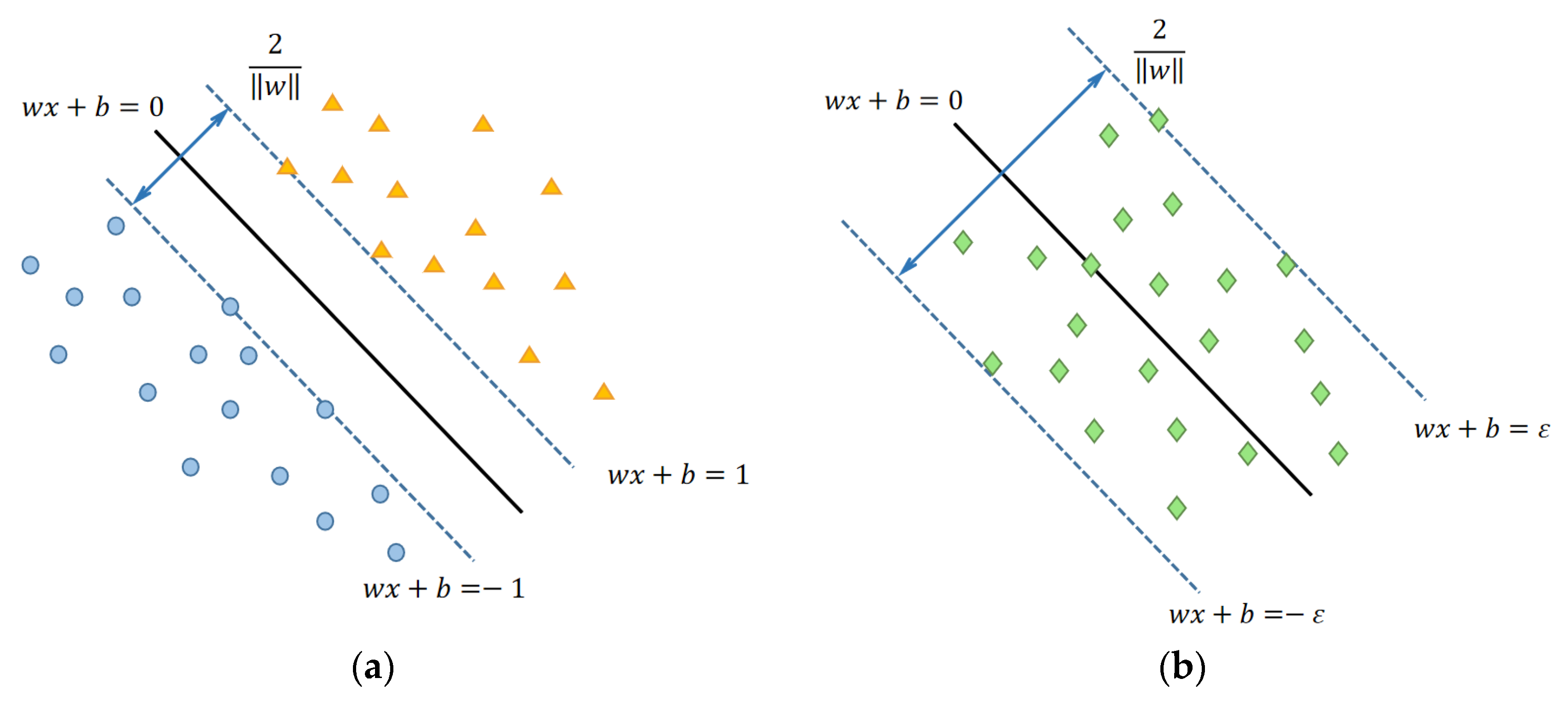
SVR fits data by constructing an optimal hyperplane in a high-dimensional feature space. Figure 2 illustrates the fundamental concepts of SVM and SVR, while Figure 3 shows how a kernel function implicitly maps the input space to a high-dimensional feature space. Support vectors are the training data points closest to the optimal hyperplane, and they determine its position. To find the separating hyperplane with the “maximum margin”, it is necessary to maximize the parameter $\gamma$ under certain constraints, as shown in Equation (9).

$$\underset{w,b}{\mathit{max} }\gamma ={\displaystyle \frac{2}{‖w‖}},s.t. y_i(w^T{x}_i+b)\ge 1,i=\mathrm{1,2},\cdots ,m,$$

(9)

where $\gamma$ is the margin between the hyperplanes, and $w$ and $b$ are the hyperplane parameters. The optimization objective for a regression problem can be transformed into Equation (10):

$$\underset{w,b}{\min } {\displaystyle \frac{1}{2}}{‖w‖}^2+C{\sum }_{i=1}^N{l}_{\epsilon }\left(f\right(x_i)-y_i),$$

(10)

where C is the regularization constant, which balances model complexity and prediction error, and $\epsilon$ is the error tolerance, which controls the sensitivity to prediction errors. The loss function, $l_{\epsilon }\left(z\right)$, is defined in Equation (11):

$$l_{\epsilon }\left(z\right)=\left\{\begin{array}{c}0,\left|z\right|<\epsilon \\ \left|z\right|-\epsilon ,\left|z\right|\ge \epsilon \end{array}\right..$$

(11)

2.2.2. Selection of the Kernel Function

By introducing a kernel function, SVR can effectively handle non-linear regression problems. Common kernel functions include Linear (LN), Polynomial (PL), Radial Basis Function (RBF), and Sigmoid (SIG) kernels, as shown in

Table 1. Kernel functions in SVR.

Kernel Function	Formula	Parameter
LN kernel	$k(x,y)=x^{T}y$	–
PL kernel	$k(x,y)={(\gamma x^{T}y+r)}^d$, d is the degree of the polynomial	$d,\gamma$
RBF kernel	$(x,y)=exp(-\gamma r^2)$$,\gamma ={\displaystyle \frac{1}{2{\sigma }^2}}$	$\gamma$
Exponential kernel	$k(x,y)=exp(-{\displaystyle \frac{‖x-y‖}{2{\sigma }^2}})$	$\sigma$
Laplacian kernel	$k(x,y)=exp(-{\displaystyle \frac{‖x-y‖}{\sigma }})$	$\sigma$
SIG kernel	$k(x,y)=tanh(\gamma x^{T}y+r)$	$\gamma ,r$

.

Research by Keerthi and Lin [49] has shown that when the RBF kernel is used, the linear kernel is no longer necessary. Generally, no studies have demonstrated that the SIG kernel achieves higher accuracy in regression problems compared to the RBF kernel [50]. Furthermore, Zhu et al. [51] found that the RBF kernel possesses better interpolation capabilities than the polynomial kernel. Therefore, in this study, the RBF kernel was selected as the kernel function for SVR.

2.3. Ensemble Learning Model

Ensemble learning significantly enhances a model’s generalization ability and robustness by combining the predictions of multiple base learners, making it particularly suitable for handling complex, non-linear, and high-dimensional data. Compared to traditional regression models, ensemble learning models can automatically capture non-linear relationships in the data and mitigate the impact of noise and outliers [52]. Common ensemble methods include Bagging, Boosting, and Stacking. Among them, RF, XGB, and LGBM have gained considerable attention in recent years due to their remarkable performance in the ML field, especially in regression problems [35,38,53]. RF, based on the Bagging principle, reduces model variance by constructing multiple decision trees. XGB, an optimized version of Boosting, utilizes a gradient boosting framework to significantly improve prediction accuracy. LGBM further enhances training efficiency, making it particularly well-suited for large-scale datasets.

2.3.1. Random Forest

RF is an ensemble learning method based on the Bagging (Bootstrap aggregating) principle, proposed by Breiman in 2001 [54]. Its core idea is to significantly improve the model’s generalization ability and robustness by constructing multiple decision trees and combining their predictions. It is especially effective for handling high-dimensional data and non-linear relationships. RF employs dual randomness (data sampling and feature selection) to effectively reduce model variance, prevent overfitting, and provide feature importance evaluation.

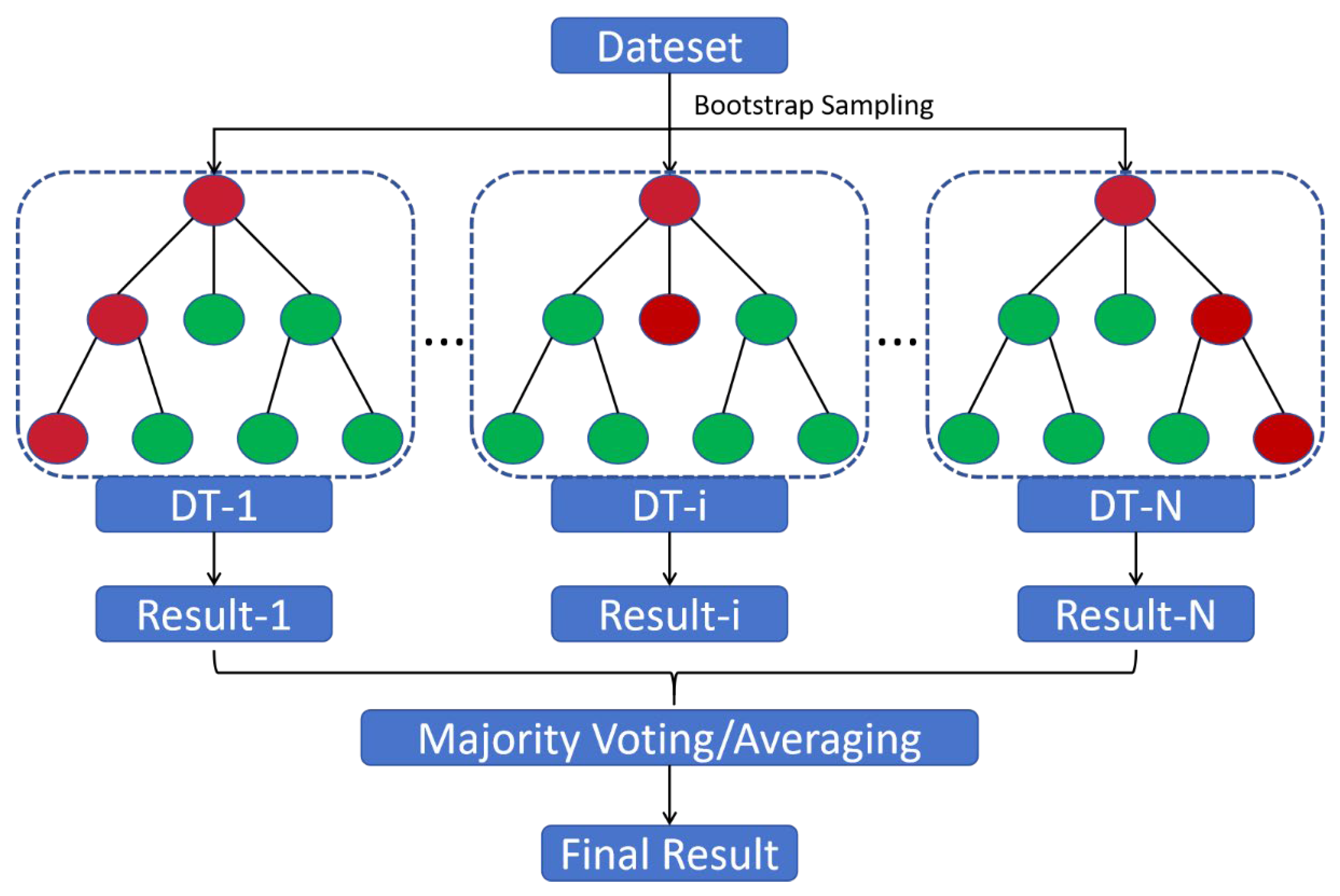
RF generates multiple sub-datasets by performing random sampling with replacement (Bootstrap sampling) on the training data. Each sub-dataset is used to train an independent decision tree. RF integrates multiple decision trees, as shown in Figure 4, each built on a bootstrapped dataset. At each node split, a random subset of features is selected. The final prediction is made by aggregating the results through voting (for classification) or averaging (for regression), thereby enhancing the model’s accuracy and generalization. For regression problems, the final prediction is the average of all tree outputs, as shown in Equation (12):

$$\widehat{y}={\displaystyle \frac{1}{N}}{\sum }_{i=1}^N{h}_i\left(x\right),$$

(12)

where $h_i\left(x\right)$ represents the prediction of the i-th tree, and $N$ is the total number of trees. RF is widely used in regression tasks, demonstrating excellent performance in scenarios involving high-dimensional data, non-linear relationships, and the need for feature importance assessment.

2.3.2. eXtreme Gradient Boosting

XGB is an ensemble learning method based on the gradient boosting framework, proposed by Chen and Guestrin in 2016 [55]. As an optimized version of the Boosting algorithm, XGBoost iteratively builds decision trees and incorporates gradient boosting techniques to significantly enhance both prediction accuracy and training efficiency. It excels in handling structured data, large-scale datasets, and complex non-linear relationships, and is widely used for classification, regression, and ranking tasks.

The core idea of XGB is to progressively reduce the model’s prediction error by iteratively constructing decision trees. The objective of each new tree is to fit the residual of the preceding model, which corresponds to the negative gradient of the loss function. Specifically, XGB defines its objective function as shown in Equation (13):

$$Obj={\sum }_{i=1}^{N}L\left(y,\widehat{y}\right)+{\sum }_{k=1}^K\Omega \left(f_k\right),$$

(13)

where $L\left(y,\widehat{y}\right)$ is the loss function that measures the difference between the true value $y$ and the predicted value $\widehat{y}$. $\Omega \left(f_k\right)$ is the regularization term used to control model complexity and prevent overfitting, defined in Equation (14). $K$ is the total number of trees.

$$\Omega \left(f_k\right)=\gamma +{\displaystyle \frac{1}{2}}\lambda {\sum }_{j=1}^T{\omega }_j^2,$$

(14)

where $\gamma$ and $\lambda$ are regularization parameters, $T$ is the number of leaf nodes in the tree, and ${\omega }_j$ is the weight of the j-th leaf node.

2.3.3. Light Gradient Boosting Machine

LGBM is a high-performance ML algorithm based on the gradient boosting framework known for its exceptional training speed and memory efficiency, making it highly suitable for large-scale datasets [56]. Its efficiency stems from two primary algorithmic innovations: a histogram-based algorithm and a leaf-wise tree growth strategy.

The histogram-based algorithm accelerates the split-finding process by discretizing continuous features into integer-valued bins and aggregating gradient statistics within each bin. This significantly reduces the computational cost and memory footprint compared to traditional methods. LGBM employs a leaf-wise growth strategy, which differs from the conventional level-wise approach. Instead of growing the tree layer by layer, it selectively splits the leaf with the maximum gain at each step. This method often leads to deeper and more accurate models with a higher risk of overfitting, which can be mitigated by tuning parameters like max_depth and min_data_per_leaf.

Like other gradient boosting models, LGBM iteratively builds decision trees to minimize loss function. Furthermore, its efficiency is enhanced by native support for parallel processing, including feature parallelism (distributing features across machines) and data parallelism (partitioning the dataset), which further accelerates model training in the distributed environments.

2.4. Hyperparameter Optimization Methods for Models

2.4.1. Grid Search

Grid search is a common hyperparameter optimization strategy. Its core principle involves creating a parameter grid from the Cartesian product of hyperparameter values and evaluating each combination to find the best-performing one. This method systematically traverses a predefined parameter space and is intuitive to implement [57].

The suitability of a grid search depends on the model’s characteristics. For SVR, which has a small number of core hyperparameters (e.g., C, γ), a grid search can efficiently find a satisfactory solution within a manageable computational cost.

However, the limitations of a grid search are significant, as its computational complexity grows exponentially with the number of hyperparameters [57]. For complex models like RF, XGB, and LGBM, which have numerous interacting parameters, this leads to a prohibitively large number of combinations and a sharp decline in optimization efficiency. The method’s reliance on manually defined ranges and its inability to learn from past evaluations further limit its effectiveness for large-scale optimization tasks compared to adaptive methods [57,58].

2.4.2. Particle Swarm Optimization

PSO is a stochastic optimization algorithm inspired by swarm intelligence, specifically the collective foraging behavior of bird flocks [59]. The algorithm seeks the optimal solution by simulating the flight of particles in a solution space. Each particle’s position represents a candidate solution (i.e., a hyperparameter combination), while its velocity and position describe its state. During the iterative process, particles dynamically adjust their flight velocity based on their own best-known position (pbest) and the swarm’s best-known position (gbest), gradually converging towards the optimal solution. The velocity and position update formulas are as follows:

$$\left\{\begin{array}{c}{v}_{i,d}^{t+1}=\omega v_{i,d}^t+c_1{r}_1\left({pbest}_{i,d}-x_{i,d}^t\right)+c_2{r}_2\left({gbest}_d-x_{i,d}^t\right)\\ x_{i,d}^{t+1}=x_{i,d}^t+v_{i,d}^{t+1}\end{array}\right.,$$

(15)

where $v_{i,d}^t$ and $x_{i,d}^t$ are the velocity and position of the i-th particle in the d-th dimension at iteration t. $\omega$ is the inertia weight, controlling the influence of the particle’s previous velocity. $c_1$ and $c_2$ are the learning factors, regulating the particle’s tendency to move towards its personal and global best positions, respectively. $r_1$ and $r_2$ are random numbers in the range [0, 1], enhancing the randomness of the search.

The advantages of PSO include its strong global search capability, simple parameter settings, and independence from gradient information, making it suitable for high-dimensional and non-convex optimization problems [59]. The algorithm converges relatively quickly, which is beneficial when prior knowledge of hyperparameter ranges is limited.

In hyperparameter optimization, PSO demonstrates good applicability for models like RF, XGB, and LGBM [60]. For these models, which have numerous interacting hyperparameters, PSO’s collaborative and stochastic search can quickly locate promising regions in a large parameter space, avoiding the computational waste of grid search. By dynamically adjusting particle trajectories, PSO rapidly focuses on potentially optimal parameter regions, reducing the risk of becoming trapped in local optima and making it highly effective for finding quality solutions within limited computational budgets.

2.4.3. Bayesian Optimization

BO is an adaptive hyperparameter optimization method based on Bayes’ theorem. Its core idea is to build a probability model to describe the mapping between hyperparameters and model performance to efficiently guide the search for the optimal combination [61]. Unlike grid search or PSO, BO leverages previously evaluated information by continuously updating its probability model for a more directed exploration of the parameter space.

The core components of BO include a probability surrogate model (often a Gaussian Process) and an acquisition function. The process begins with a prior distribution over the objective function. This prior is updated with new observations (i.e., a hyperparameter combination and its corresponding performance) to obtain a posterior distribution, as described by Bayes’ formula:

$$P\left(\theta \left|y\right.\right)={\displaystyle \frac{P\left(y\left|\theta \right.\right)P\left(\theta \right)}{P\left(y\right)}},$$

(16)

where $\theta$ is the hyperparameter combination, $y$ is the model performance metric, $P\left(\theta \right)$ is the prior distribution, $P\left(y\left|\theta \right.\right)$ is the likelihood function, and $P\left(\theta \left|y\right.\right)$ is the posterior distribution. The acquisition function (e.g., Expected Improvement (EI), Probability of Improvement (PI)) then uses the posterior distribution to select the next hyperparameter combination for evaluation. Its goal is to balance exploration (of under-explored parameter regions) and exploitation (of known high-performance regions). For example, the formula for EI is $EI\left(\theta \right)=E\left[\mathrm{m}\mathrm{a}\mathrm{x}(y\left(\theta \right)-y_{\mathrm{b}\mathrm{e}\mathrm{s}\mathrm{t}},0)\right]$, where $y_{\mathrm{b}\mathrm{e}\mathrm{s}\mathrm{t}}$ is the best model performance found so far.

In the hyperparameter optimization of RF, XGB, and LGBM, BO shows significant advantages [62]. For these models, which are often sensitive to complex hyperparameter interactions, BO’s ability to capture these relationships through its probability model allows it to find good solutions with fewer evaluations. As the number of hyperparameters increases, the efficiency advantage of BO becomes more prominent, often requiring an order of magnitude fewer evaluations than grid search and significantly less than PSO in a complex parameter space [57,58,63].

2.5. 10-Fold Cross-Validation

When the sample size is small, different splits of the training subset can lead to significantly different computational results, even when the model uses the same hyperparameters [64]. Insufficient sample size can result in inadequate data distribution, which in turn affects the distribution of the resulting subsets and leads to unstable outcomes. Common methods for selecting validation subsets include Leave-one-out, Monte Carlo random sampling, and K-fold cross-validation [65]. In studies predicting the compressive strength of cement-based materials, K-fold cross-validation is the most popular technique [66,67,68,69,70]. This technique involves dividing the data into K folds and running the model K times, and a different fold is used for validation each time to prevent overfitting.

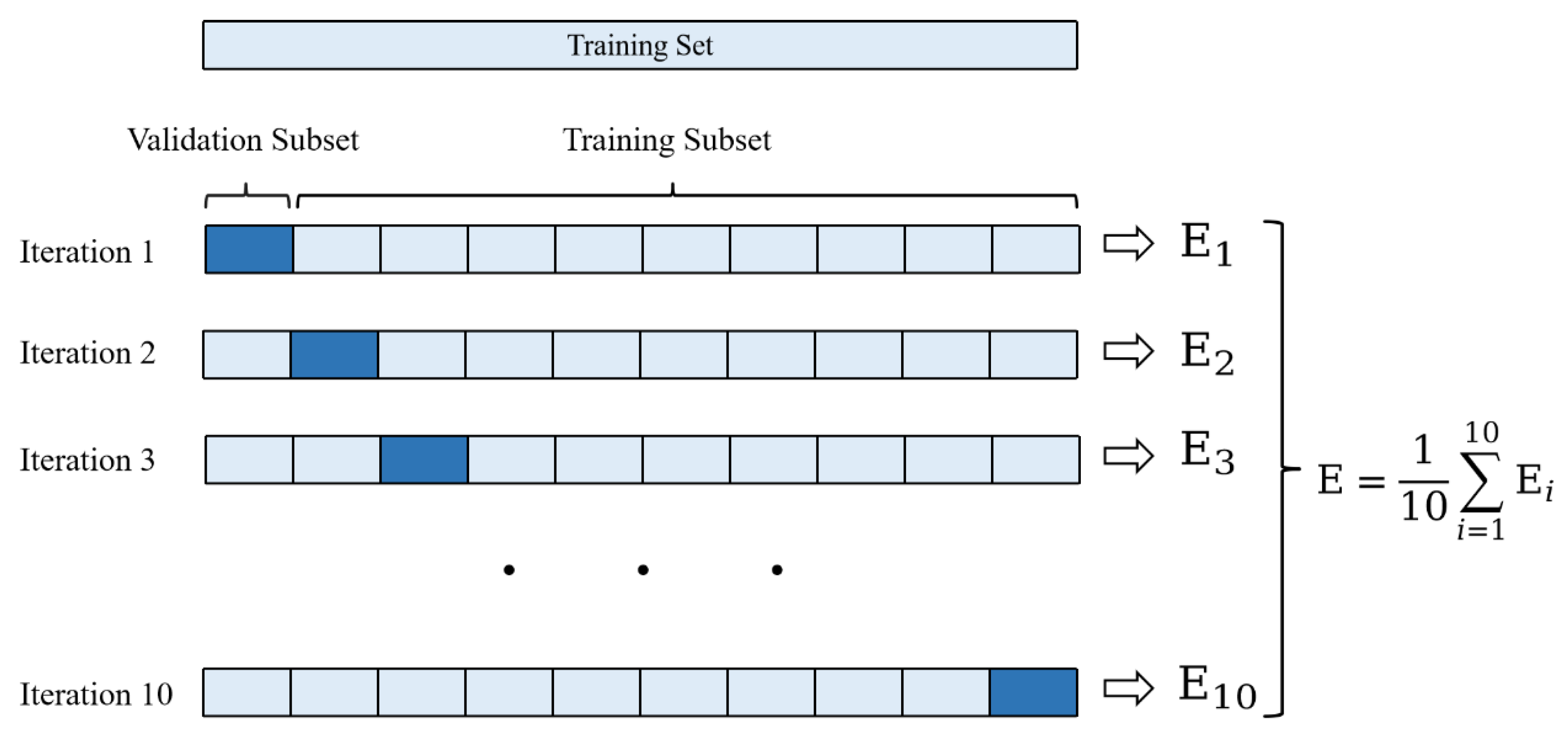
To develop a more stable and generalizable compressive strength prediction model, this study employs a 10-fold cross-validation method to mitigate the problem of overfitting. Research by Kohavi et al. has demonstrated that ten folds is the optimal number for achieving good results within an acceptable time frame [64,71]. Ten-fold cross-validation randomly divides the dataset into ten equal parts. In each round, nine parts are used for model training, and the remaining part is used for validation. The process is repeated for ten rounds, as shown in Figure 5, ensuring that all data samples are used for both training and validation. Finally, the overall model performance is evaluated by averaging the performance metrics of the 10 models.

2.6. Performance Evaluation Metrics for Models

To comprehensively evaluate the predictive performance of the algorithms, several evaluation metrics were selected, including Maximum Error (ME), Root Mean Square Error (RMSE), Mean Absolute Error (MAE), Mean Absolute Percentage Error (MAPE), and the Coefficient of Determination (R²) [72,73,74].

ME represents the maximum absolute difference between the predicted and true values. It is sensitive to outliers and can effectively capture the worst-case prediction scenario in the sample. RMSE measures the deviation between predicted and true values, also known as the standard error, and it can reflect the overall performance of the model. MAE is the average of the absolute errors between the predicted and true values, and a smaller value indicates a better model fit. MAPE is the average of the percentage of absolute errors relative to the true values, reflecting prediction accuracy in terms of relative error. R² indicates the proportion of the variance in the dependent variable, that is predictable from the independent variables. Its value ranges from 0 to 1, with values closer to 1 indicating a better regression fit.

Their calculation formulas are shown in Equations (17)–(21), where $f\left(x_i\right)$ is the predicted value, $y_i$ is the measured or target value, $\overline{y_i}$ is the average of the measured values, and m is the number of samples in the dataset.

$$ME=max\left(\left|f\left(x_i\right)-y_i\right|\right),$$

(17)

$$RMSE=\sqrt{{\displaystyle \frac{1}{m}}{\sum }_{i=1}^m{\left(f\right(x_i)-y_i)}^2},$$

(18)

$$MAE={\displaystyle \frac{1}{m}}{\sum }_{i=1}^m\left|f\left(x_i\right)-y_i\right|,$$

(19)

$$MAPE={\displaystyle \frac{1}{m}}{\sum }_{i=1}^m\left|{\displaystyle \frac{f\left(x_i\right)-y_i}{y_i}}\right|\times 100\mathrm{\%},$$

(20)

$$R^2=1-{\displaystyle \frac{{\sum }_{i=1}^m{\left(f\right(x_i)-y_i)}^2}{{\sum }_{i=1}^m{(\overline{y_i}-y_i)}^2}}.$$

(21)

Additionally, the engineering metric a20-index is also used for model reliability assessment [75]. The a20-index intuitively reflects the proportion of samples where the deviation between predicted and measured values is within a 20% range. For a perfect prediction model, the a20-index should be 1. In the field of engineering, accurate predictions and model reliability are crucial for design and decision-making. The a20-index can clearly evaluate the model’s prediction accuracy, thereby enhancing the assessment of the model’s reliability.

$$a20-index={\displaystyle \frac{m20}{M}}.$$

(22)

In general, superior model performance is indicated by higher R² and a20-index values, coupled with lower ME, RMSE, MAE, and MAPE values.

3. Dataset Establishment

3.1. Data Collection

This study employed Systematic Search Flow [76,77] for literature search and data extraction. All the literature published between 2004 and 2024 was retrieved, and relevant papers with clearly described experimental conditions and detailed CNT material parameters were selected. The most commonly used cement type was Ordinary Portland cement. In some studies, supplementary cementitious materials such as fly ash or silica fume were also included, reflecting diverse mix designs. The CNTs were predominantly MWCNTs, with their key physical properties (diameter, length) included as features in our model. From these, 429 valid data samples were extracted.

3.2. Distribution of Data Samples

In this study, a feature system was systematically constructed from six dimensions: matrix mix proportions, CNT material parameters, CNT dispersion process, CNT interfacial modification, specimen geometry and size, and curing time. This approach aims to comprehensively cover the mechanisms influencing the compressive strength of CNT-reinforced concrete.

Parameters of the cement matrix mix proportion (water–cement ratio, sand–cement ratio) were prioritized as feature variables, as they directly determine the cement hydration process and the aggregate interface structure, which are critical for the mechanical properties of concrete [73]. CNT material parameters such as the mass percentage of CNT to cement, CNT outer diameter, CNT inner diameter, and CNT length were included as core features. These parameters not only quantify the physical state of the nano-reinforcement phase but also significantly influence its dispersion efficiency and stress transfer effectiveness in the cement matrix by modulating key indicators like specific surface area and aspect ratio [7]. To accurately reflect the impact of the preparation process, parameters like sonication duration and surfactant type (see

Table 2. Types of surfactants.

Variable Code	Surfactant
AA	no surfactant used
PC	Polycarboxylate
GA	Gum Arabic
PVPPD	Polyvinylpyrrolidone and Polyether modified silicone oil defoamer
PCE	Polycarboxylic Ether
AMPGE	Aromatic modified polyethylene glycol ether
PVP	Polyvinylpyrrolidone
CMC	Carboxyl-methyl cellulose
DP	Dolapix PC67 series dispersant
HH	H2SO4 and HNO3 mixture

) were introduced as feature variables. Such parameters directly affect the enhancement efficiency by altering the agglomeration state of CNTs. Simultaneously, as some CNT samples were chemically modified to introduce polar functional groups, treatments involving hydroxyl, carboxyl, and thiazole groups were included in the feature space. These chemical modifications fundamentally improve the macroscopic mechanical properties of the composite by enhancing the interfacial bonding strength between CNTs and the cement matrix. Furthermore, the specimen’s geometric shape (e.g., cube or prism) and dimensions (e.g., side length, height) were also included, as they directly influence the compressive strength test results. Curing age was introduced as a crucial time-dependent variable, because the strength of concrete develops continuously over time with the cement hydration reaction. Compressive strength was selected as the target variable.

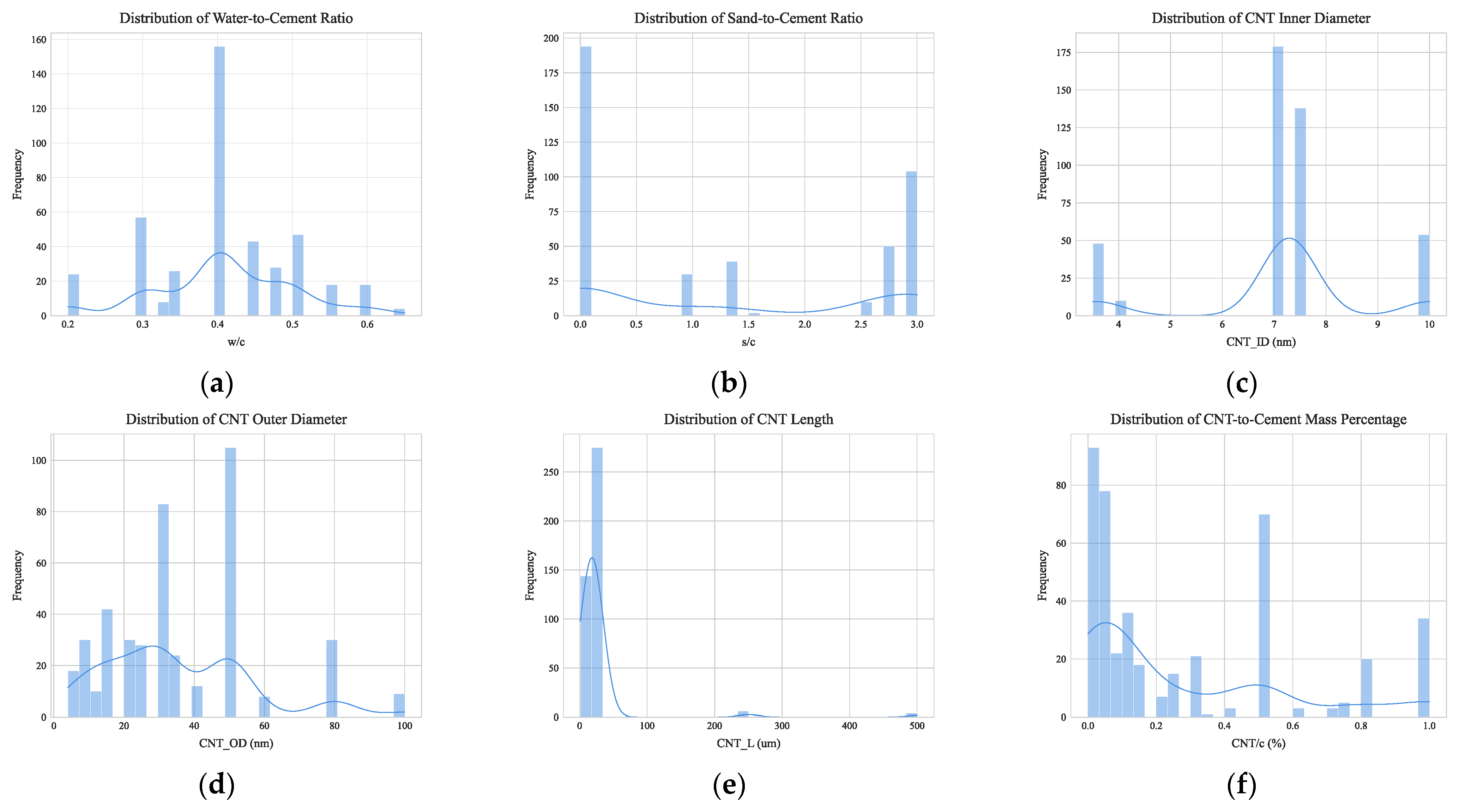
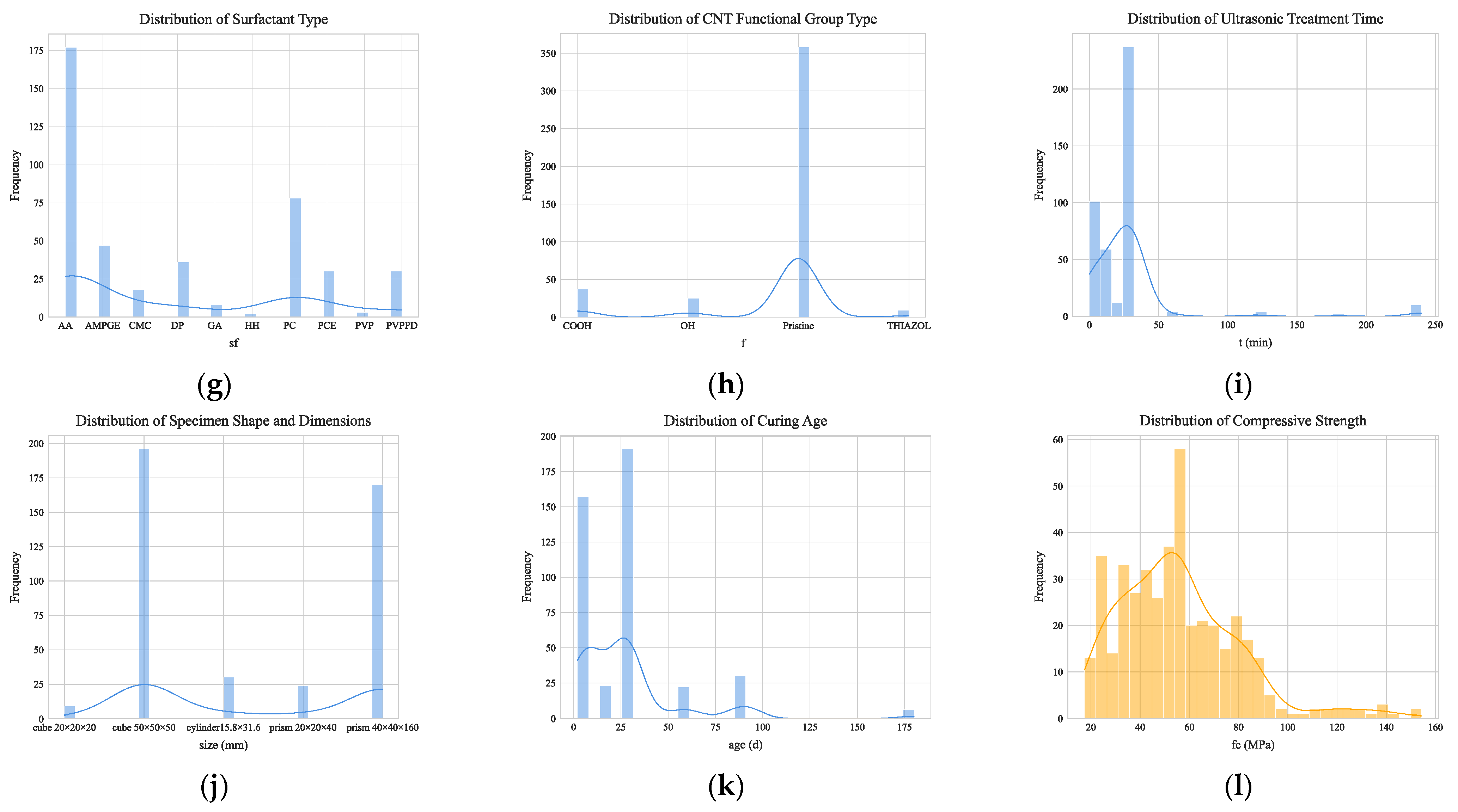
The codes, units, and value ranges for all variables are shown in

Table 3. The codes, units, and value ranges for all variables.

Variable	Code	Unit	Value Range
Water–cement ratio	w/c	–	0.2–0.65
Sand–cement ratio	s/c	–	0.0–3.0
CNT inner diameter	CNT_ID	nm	3.5–10.0
CNT outer diameter	CNT_OD	nm	4.0–100.0
CNT length	CNT_L	um	1.0–500.0
Mass ratio of CNT to cement	CNT/c	%	0.0–1.0
Surfactant type	sf	–	AA, PC, GA, PVPPD, PCE, AMPGE, PVP, CMC, DP, HH
CNT functional group	f	–	OH, COOH, Thiazole, Pristine 1
Sonication duration	t	min	0.0–240.0
Specimen parameter	size	mm	prism 40 × 40 × 160, prism 20 × 20 × 40, cube 50 × 50 × 50, cube 20 × 20 × 20, cylinder 15.8 × 31.6
Curing time	age	d	2.0–180.0
Compressive strength	fc	MPa	17.4–154.4

¹ “Pristine” indicates no chemical treatment for the CNTs.

. The distribution characteristics of the 12 feature variables are analyzed in Figure 6.

(1) Matrix mix proportions. The water–cement ratio shows a unimodal distribution centered at 0.4 (29.4%), with the 0.3–0.5 range covering 53.6% of the samples. Values of 0.2 (5.6%) and 0.6 (4.2%) provide data for the model to capture performance boundaries. The maximum sand–cement ratio is 3.0, corresponding to 103 samples. However, the majority of samples use a much smaller ratio, with values ranging from 0 to 0.2.

(2) CNT material parameters. Over 70% of CNT inner diameters are concentrated in the 7–7.5 nm range, with the remainder mainly at the extremes of 3.5 nm and 10 nm. In contrast, the distribution of CNT outer diameters is more uniform, with about 44% in the 30–50 nm range. For CNT length, 71.3% of samples use short lengths of 15–20 μm, while very few researchers use lengths over 200 μm. The mass percentage of CNT to cement varies from 0 to 1.0% with a wide range of values, which helps the model analyze the effect of different CNT dosages. The 0–0.3% dosage range and the 0.5% dosage are research hotspots.

(3) CNT dispersion process. Sonication time exhibits a unimodal distribution centered at 30 min (55.2%). Short-duration treatments of 0–20 min cover 39.2% of samples, with 5 min and 15 min as secondary concentration intervals. Long-duration treatments over 30 min account for only 4.7%, providing data to capture performance boundaries. Among surfactants, PC (28.6%) and AA (25.3%) are the most common, together covering 53.9% of samples. AMPGE (13.8%), PCE (11.2%), and DP (9.5%) follow, forming the mainstream selection. Types like PVP (1.8%) and HH (0.9%) have very low proportions.

(4) CNT interfacial modification. The choice of CNT functional groups shows a clear concentration trend. Pristine (no chemical treatment) is the most common, covering about 70% of samples. The COOH functional group accounts for about 15%, the OH group slightly less for about 12%, and the Thiazole group has the lowest proportion of about 3%.

(5) Specimen geometry and size. Cube 50 × 50 × 50 (cube, 50 × 50 × 50 mm) is the most common, covering about 50% of samples. Prism 40 × 40 × 160 (prism, 40 × 40 × 160 mm) is the next, at about 30%. Cylinder 15.8 × 31.6 (cylinder, 15.8 × 31.6 mm, diameter × height) accounts for about 10%. Cube 20 × 20 × 20 and prism 20 × 20 × 40 have the lowest proportions, each at about 5%.

(6) Curing time. The distribution of curing age shows a distinct concentration. The 28-day curing age is the most frequent, covering about 45% of samples. Medium-term ages of 7–14 days are next, totaling about 35%. Short-term ages of 3 days or less account for about 11%. Long-term ages of 58 days and above (including 58, 60, 90, and 180 days) have the lowest proportion, totaling about 16%.

3.3. Data Preprocessing

In the entire dataset, six features had missing data: w/c, CNT_ID, CNT_OD, CNT_L, sf, and t. The specific details of the missing values are shown in

Table 4. Missing values in the dataset.

Feature	Number of Missing Values	Completeness (%)
w/c	6	98.60
CNT_ID	39	90.91
CNT_OD	18	95.80
CNT_L	31	92.77
sf	19	95.57
t	30	93.01

.

Different strategies were adopted for different features with missing data. For the w/c, given its significant impact on the strength of cement-based materials and the small number of missing samples (only six), these samples were directly discarded. For the geometric dimensions of CNTs (CNT_ID, CNT_OD, CNT_L), the mean value of all samples was used to maintain data consistency and integrity. For samples with sonication duration missed, it was assumed that sonication was not used, as it is not explicitly stated in the original literature. Similarly, samples with a missing surfactant type were assumed to have “no surfactant used”.

The dataset contains three categorical features: specimen parameter (size), surfactant type (sf), and CNT functional group (f). The size feature was split into three new variables: shape type (cyl), side length or diameter (B), and height (H). The sf and f were processed using one-hot encoding to be converted into new variables. The one-hot encoding results for the functional group types are detailed in

Table 5. The one-hot encoding results for the functional group types.

Functional Group	f_OH	f_COOH	f_Thiazol
Pristine	0	0	0
OH	1	0	0
COOH	0	1	0
Thiazole	0	0	1

.

To eliminate the influence of different scales and value ranges among variables, all data were normalized. This not only improves model accuracy but also accelerates the convergence speed when using optimization algorithms like gradient descent. Common normalization methods include Min-Max normalization and Z-score normalization. Given that Z-score normalization demonstrates better robustness against noise and outliers in the dataset, this method was chosen. The specific normalization formula is as follows:

$$z={\displaystyle \frac{x-\mu }{\sigma }},$$

(23)

where $z$ is the normalized data, $x$ is the original data, $\mu$ is the mean of the data, and $\sigma$ is the standard deviation. After Z-score normalization, the data has a mean of 0 and a standard deviation of 1.

Finally, the dataset was randomly shuffled. It was then split into a training set (80%) to fit the model parameters and a test set (20%). To select an appropriate model and determine its hyperparameters, the training set was further subjected to ten-fold cross-validation, dividing it into training and validation subsets to prevent overfitting [78].

3.4. Feature Correlation Analysis

The primary purpose of conducting a feature correlation analysis is to explore the interactions between different features and to identify those that have a significant impact on the target variable (the compressive strength of concrete in this study). First, identifying features highly correlated with the target variable can simplify the model and improve prediction accuracy. Concurrently, detecting strong correlations between features helps to avoid multicollinearity, preventing model instability and overfitting. Furthermore, analyzing the relationships between features allows for the identification of redundant and essential features, enabling efficient data preprocessing and providing a crucial theoretical basis for model construction and optimization.

In the feature correlation analysis, the color intensity represents the degree of correlation: red indicates a positive correlation, and blue indicates a negative correlation. The deeper the color, the stronger the correlation. The analysis results, as shown in Figure 7, reveal that the sand–cement ratio and water–cement ratio exhibit the highest positive correlation, with a coefficient of 0.58. This is likely due to their interdependence in concrete preparation and performance. For instance, an increase in the water–cement ratio often requires a corresponding increase in the sand proportion to ensure uniform mixing. Conversely, the width or diameter of the specimen and the shape type show the highest negative correlation, with a coefficient of −0.65. This is mainly because the dimensions of cylindrical specimens in the dataset are limited to a single specification (“cylinder 15.8 × 31.6”), leading to an uneven sample distribution. Additionally, all samples using PCE-type surfactants have a CNT inner diameter of 3.5 nm. This skewed sample distribution results in a correlation coefficient of −0.60 between the CNT inner diameter and the surfactant PCE. The water–cement ratio is negatively correlated with compressive strength, with a coefficient of −0.59, which is consistent with findings from previous research [79]. Apart from these feature pairs, most other pairs show low correlation coefficients, indicating weak relationships between them, although a few are elevated due to the uneven sample distribution in the dataset.

4. Results and Discussion

4.1. Traditional Regression Models

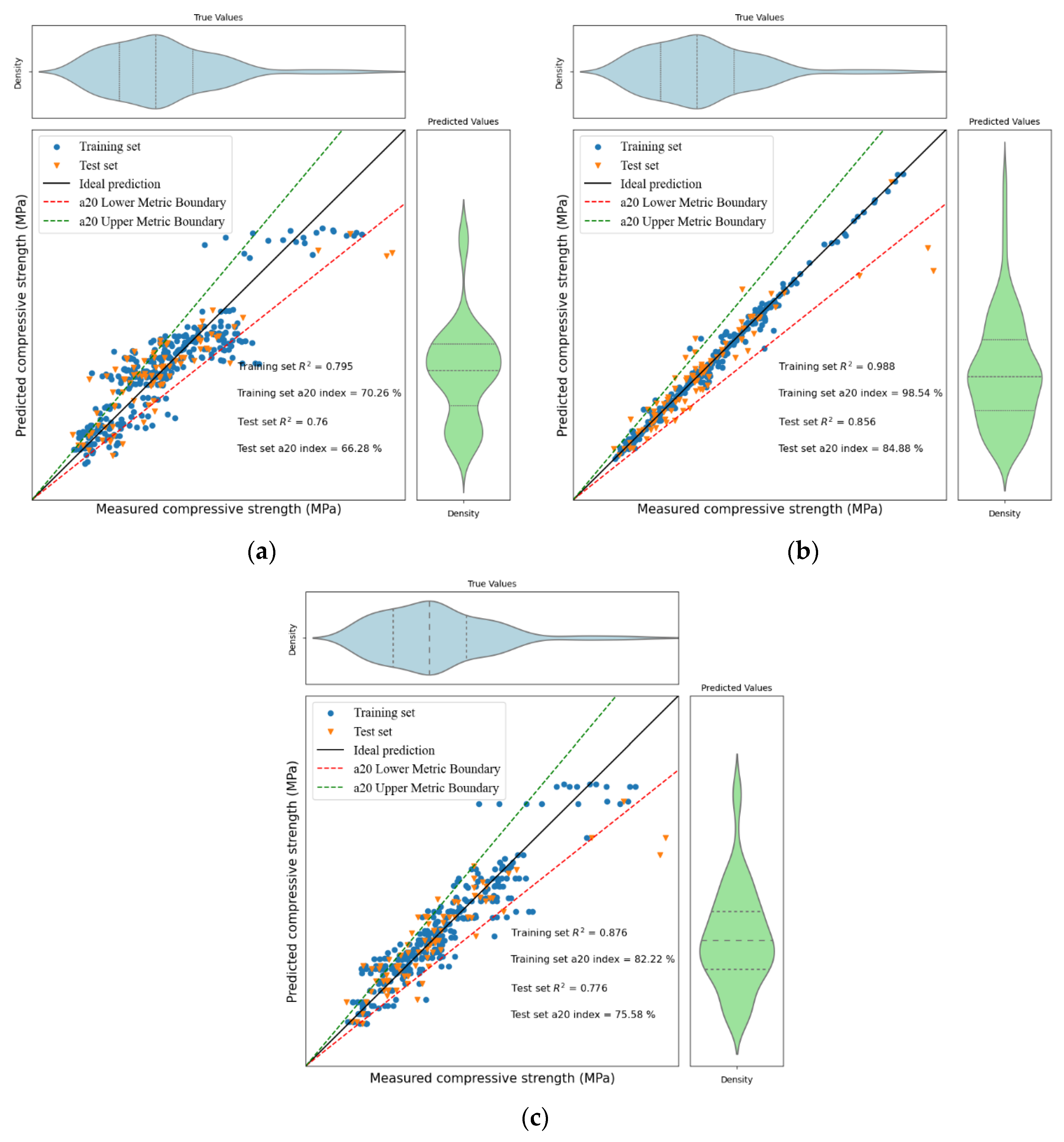
Figure 8 displays the fitting plots for the three traditional regression models, MLR, MPR, and MARS, in which the violin plots in the upper part of the figure show the distribution characteristics of the actual data, and those on the right side illustrate the distribution characteristics of the predicted data. The dashed lines inside the violin plots represent their quartiles (first quartile, median, lower quartile). In terms of prediction accuracy and generalization ability, the three models show significant differences. The MPR model performed the best, achieving an R² of 0.988 and an a20-index of 98.54% on the training set. Its data points closely follow the ideal prediction line, indicating that the model can accurately capture the patterns in the training data. On the test set, it obtained an R² of 0.856 and an a20-index of 84.88%. Although there was a reduction in performance, the values remained high, demonstrating that the model balances both prediction accuracy and generalization ability. The MARS model achieved an R² of 0.876 and an a20-index of 82.22% on the training set, with its data points showing some dispersion but an overall aligned trend. However, on the test set, the R² dropped to 0.776 and the a20-index to 75.58%, indicating an amplification of prediction error. Finally, the MLR model exhibited the weakest performance. On the training set, it achieved an R² of only 0.795 and an a20-index of 70.26%, with highly scattered data points, which suggests the model insufficiently captured the training data patterns. On the test set, the R² was 0.76 and the a20-index was 66.28%, revealing significant shortcomings in both prediction accuracy and generalization ability.

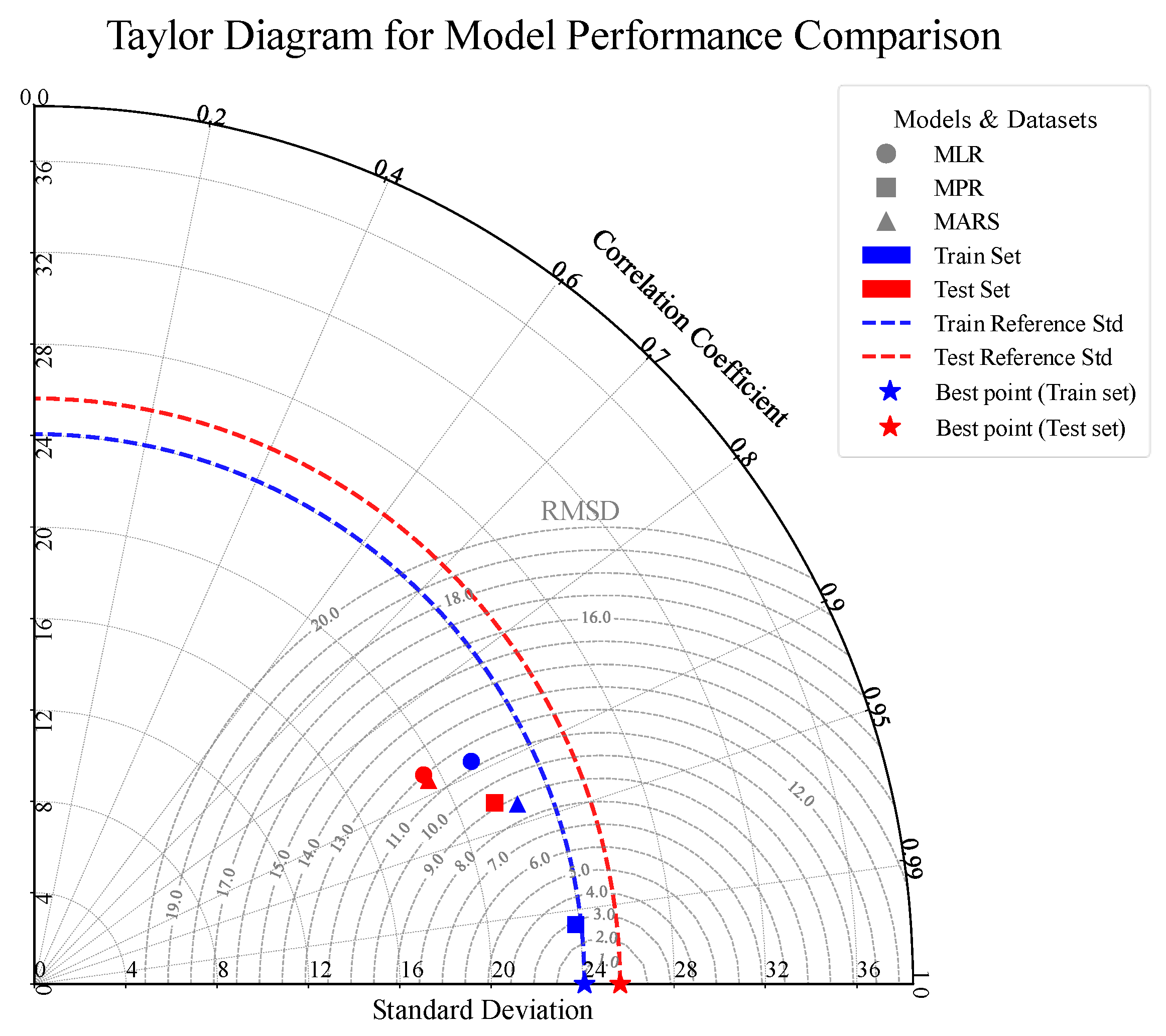
Figure 9 and Figure 10 present the normalized radar charts and the Taylor diagram, respectively, for the performance evaluation of the three traditional regression models. On both the training and test sets, the MPR model’s metrics are significantly superior to those of MLR and MARS, as shown in Figure 9 and Figure 10, demonstrating more stable and higher predictive performance.

4.2. Support Vector Regression

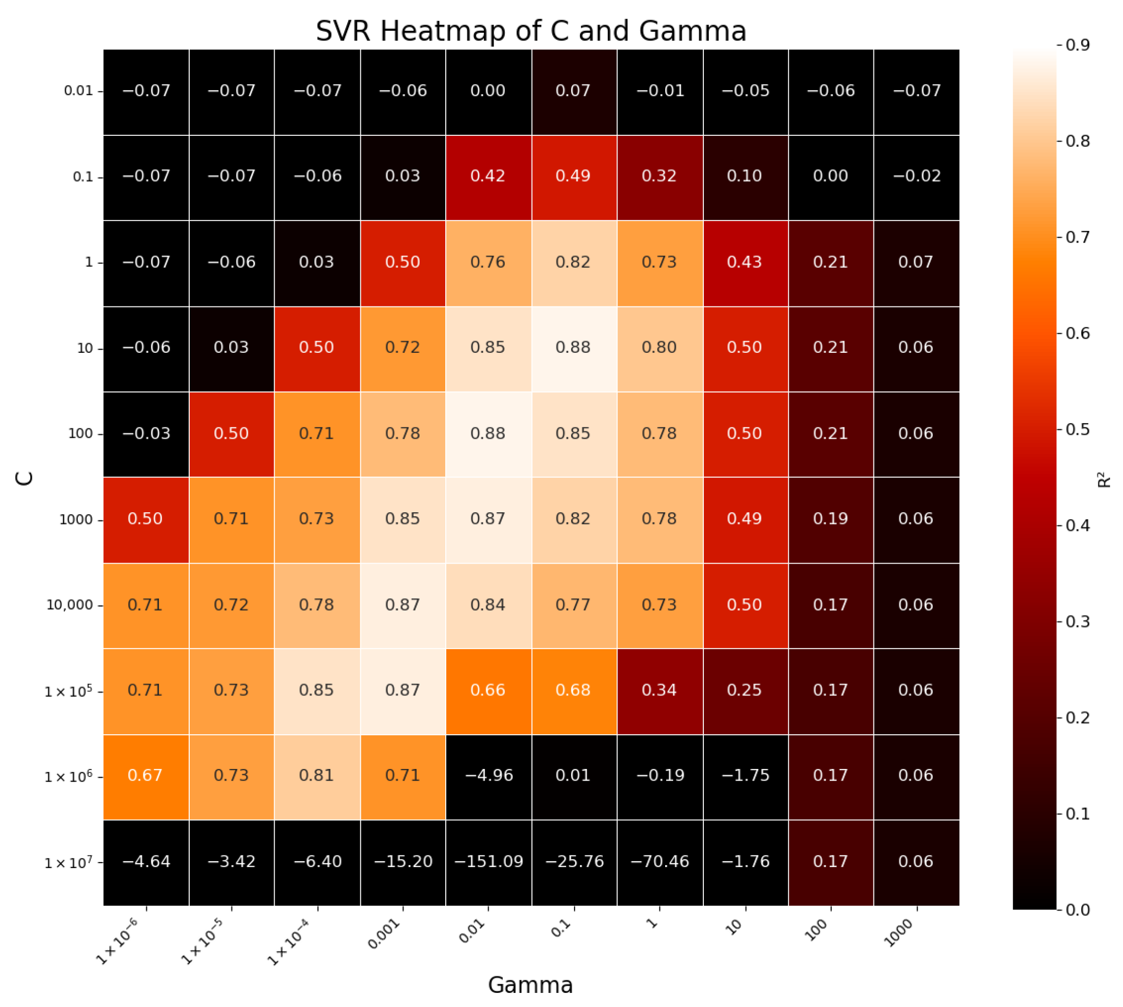
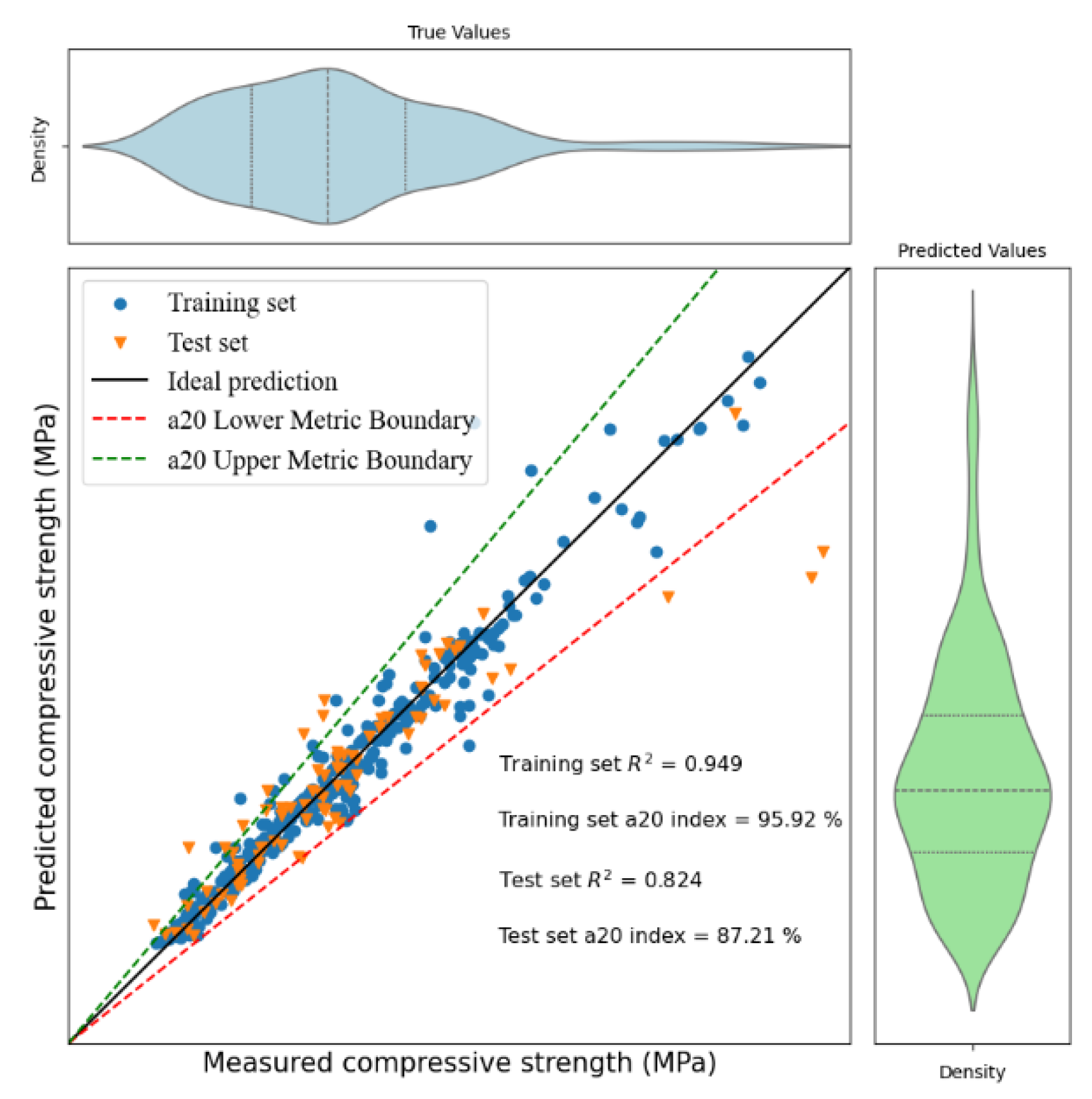
After selecting RBF as the kernel for the SVR model, two hyperparameters needed to be determined: the regularization constant C and gamma ($\gamma$). Given the small number of hyperparameters, the grid search method was employed for tuning. The results of the hyperparameter tuning, as shown in Figure 11, revealed that the model achieved a higher R² on the validation set when $\gamma$ was in the range of 0.01 to 0.1 and C was in the range of 10 to 100. The hyperparameter combination of $\gamma$ = 0.01 and C = 100 was selected. The final fitting results of the model are shown in Figure 12.

As shown in Figure 12, the SVR model achieved an R² of 0.949 on the training set and 0.824 on the test set, indicating good prediction performance in both cases. The prediction metrics of the tuned SVR model (

Table 6. Prediction metrics of the SVR model after hyperparameter tuning.

Dataset	ME	MAE	RMSE	R2	MAPE (%)	a20
Training set	1.873	0.140	0.051	0.949	1.085	0.959
Test set	2.331	0.245	0.197	0.824	1.170	0.872

) show that its performance is superior to the MLR and MARS models and is comparable to that of the MPR model. Although the R² of the SVR on the test set is slightly lower than that of the MPR, the SVR is less time-consuming in terms of computational efficiency (the computation time of the SVR is 256 s and that of the MPR is 477 s), making it a practical and excellent algorithm.

4.3. Ensemble Learning Models

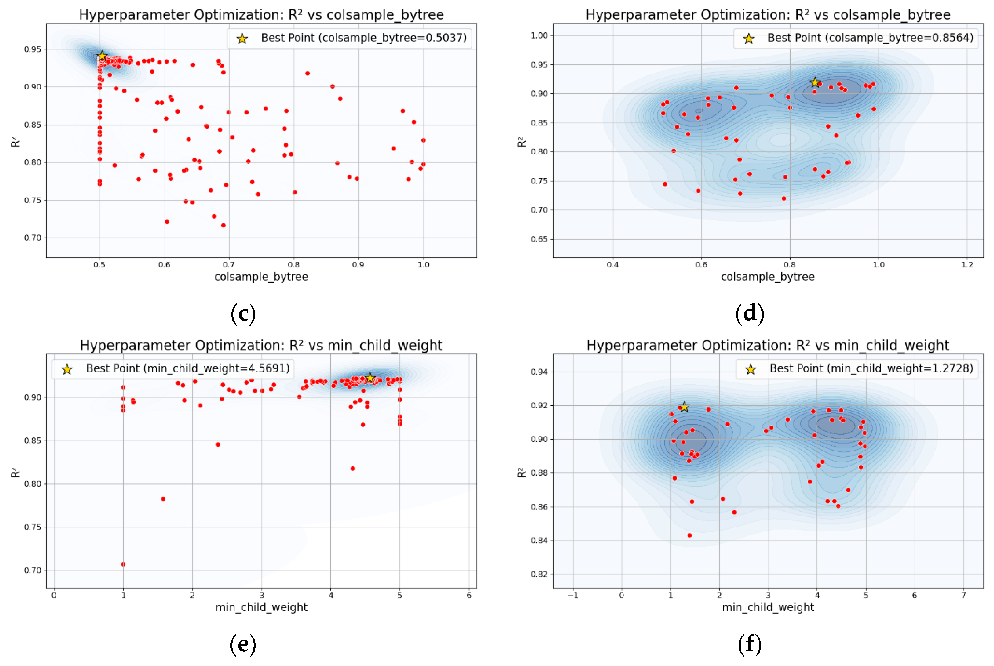
In this study, two algorithms (PSO and BO), were selected to perform hyperparameter optimization for three models: RF, XGB, and LGBM. The specific hyperparameter types, their corresponding search ranges, optimal values, and computation times are detailed in

Table 7. Hyperparameter optimization results for the three ensemble learning models.

Model	Hyperparameter	Search Range	Optimal Value		Computation Time (s)
			PSO	BO	PSO	BO
RF	n_estimators	[100, 1000]	502	159	2420	186
	min_samples_leaf	[1, 50]	3	1
	max_depth	[5, 50]	45	42
	max_features	[0.1, 1]	0.7030	0.9280
XGB	n_estimators	[100, 300]	134	291	156	23
	max_depth	[3, 10]	8	3
	learning_rate	[0.01, 0.3]	0.2724	0.0902
	subsample	[0.5, 1.0]	0.7475	0.6883
	min_child_weight	[1, 10]	4.9808	2.1485
	colsample_bytree	[0.5, 1.0]	0.5037	0.8564
	gamma	[0, 5]	0.0000	0.0463
LGBM	n_estimators	[100, 200]	195	179	66	24
	max_depth	[3, 10]	10	9
	learning_rate	[0.01, 0.2]	0.1895	0.1761
	subsample	[0.6, 1.0]	0.9016	0.8585
	min_child_weight	[1, 5]	4.5691	1.2728
	colsample_bytree	[0.5, 1.0]	0.9849	0.9015
	reg_alpha	[0, 1]	0.0026	0.0697
	reg_lambda	[0, 1]	0.1438	0.3148

. Figure 13 illustrates the optimization process for some of the hyperparameters in the RF, XGB, and LGBM models. In Figure 13, a deeper blue color indicates a denser concentration of parameter points selected by the optimization algorithm, which visually reveals the differences in exploration strategies between the algorithms across various parameter ranges.

Figure 13 clearly shows that the hyperparameter tuning strategies of PSO and BO differ significantly. PSO is characterized by its extensive exploration, calculating a large number of randomly generated reference points to locate the optimal hyperparameter values. While this approach can capture potential optimal solutions over a broader range, it consumes substantial computational resources, leading to lower efficiency. In contrast, BO tends to learn from existing computation results. It iteratively updates its understanding of the parameter space to focus on regions more likely to contain better solutions. This history-based and targeted search strategy allows it to narrow down the exploration scope more efficiently during the tuning process.

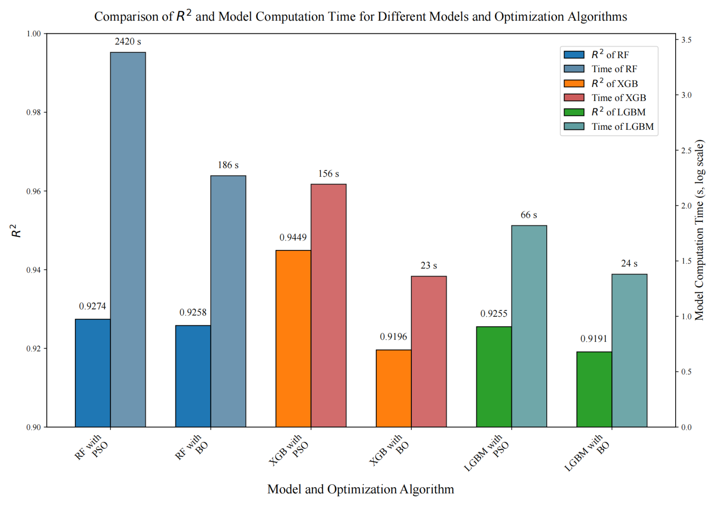
To quantitatively compare the differences between PSO and BO in terms of computation time and optimization accuracy, Figure 14 presents the R² values on the validation set and the corresponding computation times for the RF, XGB, and LGBM models optimized by both algorithms. The results show that for all three ensemble models, the R² on the validation set was higher after PSO compared to BO, indicating that PSO has an advantage in optimization accuracy. However, in terms of time consumption, BO was significantly more efficient. This was particularly prominent for the RF model, where PSO took 2420 s, while BO required only 186 s, a reduction in computation time by more than tenfold. This trade-off between accuracy and efficiency provides a direct basis for selecting an optimization algorithm in different scenarios. If the priority is to maximize the model prediction accuracy, PSO is more suitable. If computational cost is a major concern, BO is the better choice.

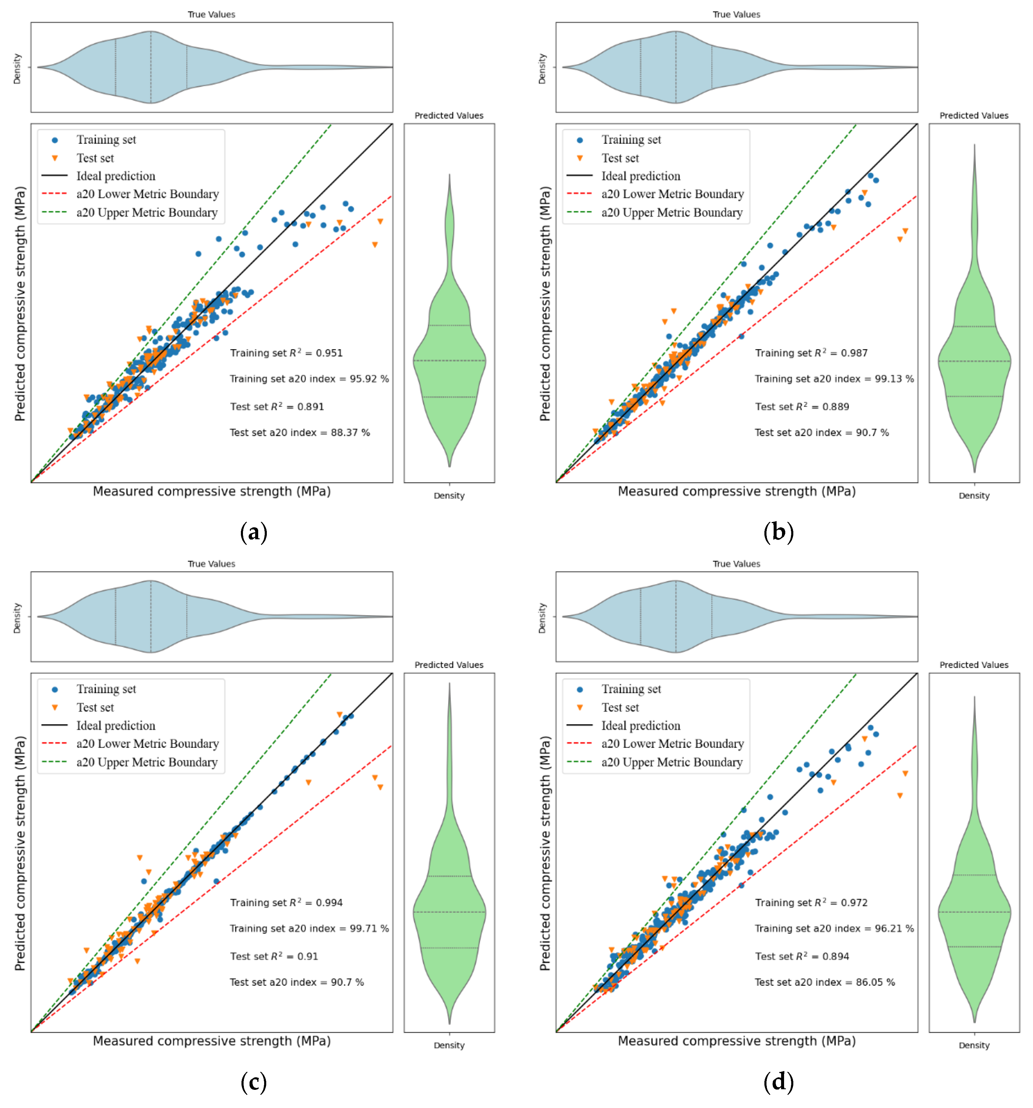
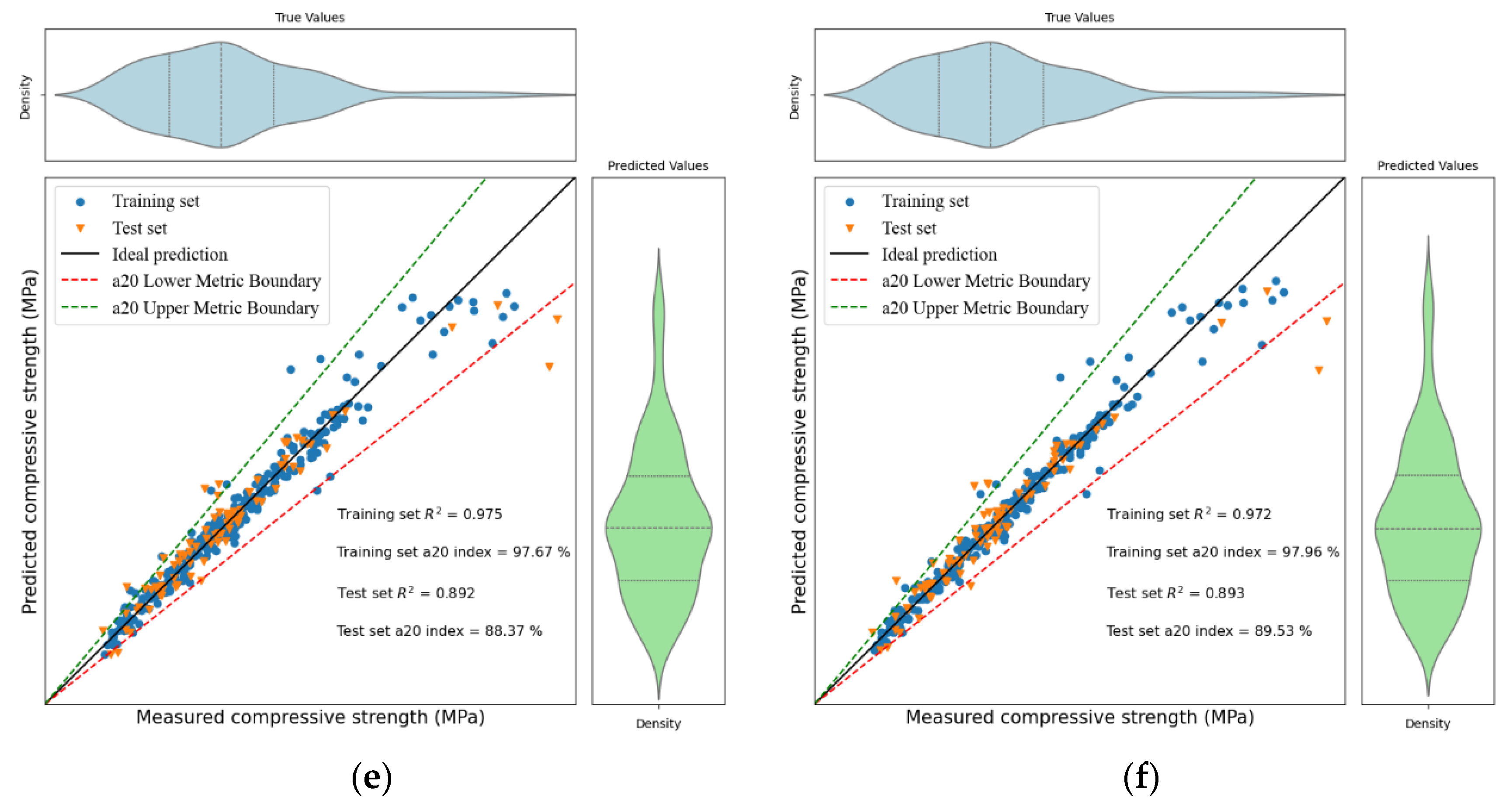
Figure 15 presents the fitting results of the three ensemble models (RF, XGB, and LGBM) after being optimized by both PSO and BO. Among them, the XGB model optimized by PSO demonstrated the best prediction performance, achieving an R² of 0.910 and an a20-index of 0.907 on the test set. Although the fitting performance of the other models was slightly inferior, their test set R² values were generally around 0.89, indicating that their overall predictive performance remained reliable. Further observation of the data point distribution in the fitting plots reveals that the slightly poorer performance of these models is mainly due to insufficient fitting accuracy for high compressive strength data. This is especially true for the RF model optimized by PSO, where data points for high compressive strength are scattered and deviate significantly from the ideal prediction line. In contrast, the XGB model optimized by PSO maintained good fitting performance for compressive strength data in both high- and low-value regions, with data points closely clustered around the ideal line, demonstrating more stable prediction ability.

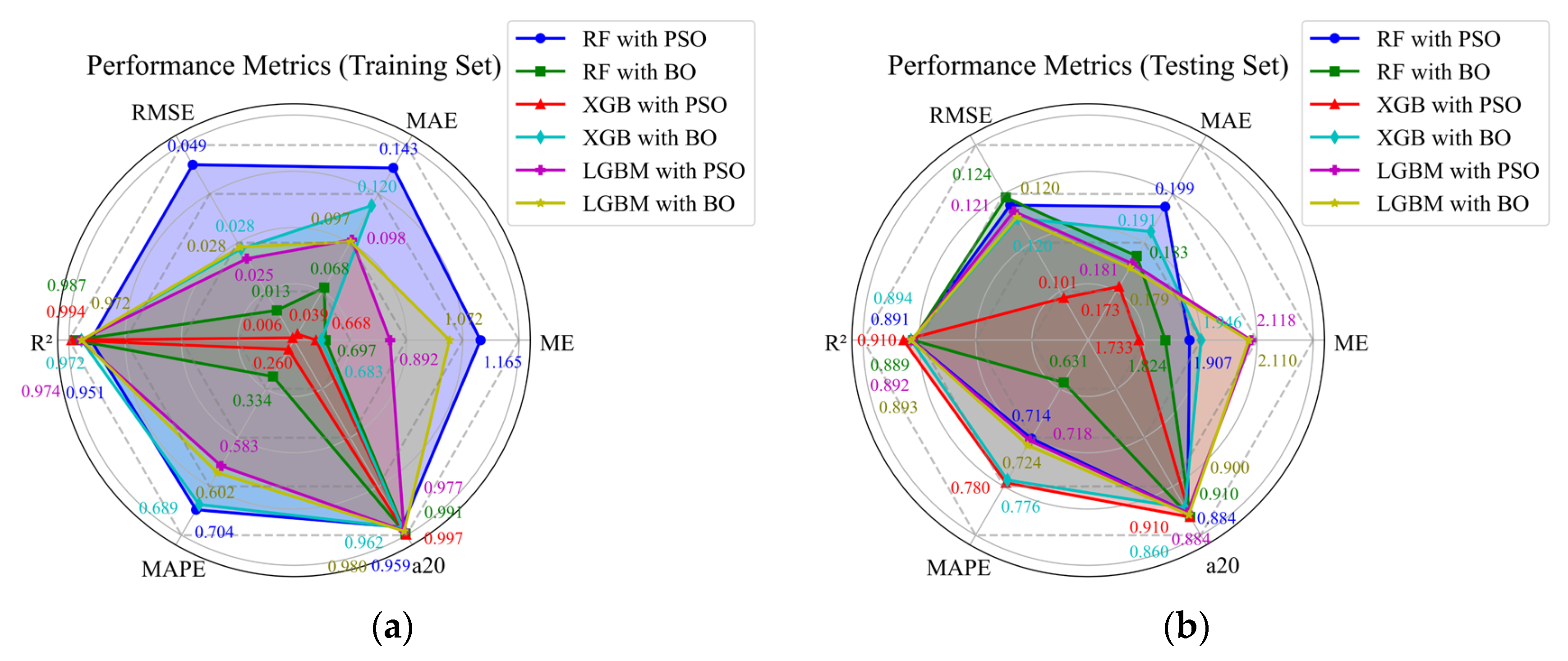
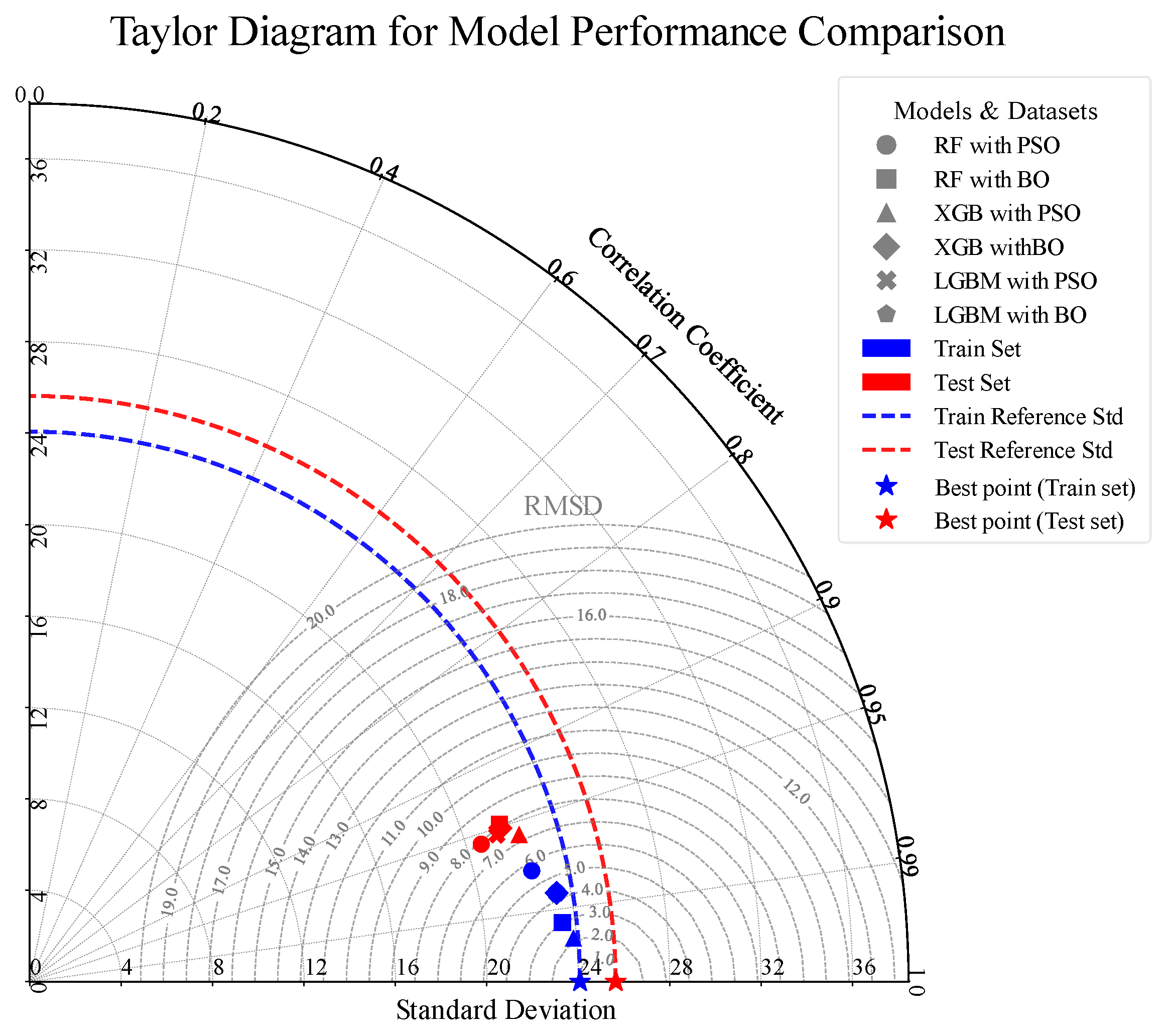
To compare the predictive performance of the three ensemble models (RF, XGB, and LGBM) after optimization by PSO and BO, normalized radar charts of the performance metrics for each model under the different tuning algorithms were provided, as shown in Figure 16. Figure 17 presents the Taylor diagram for the performance evaluation of the three ensemble learning models. As seen in the figure, the XGB model optimized by PSO performed best across all evaluation metrics on the training set. On the test set, although its MAPE was slightly higher, the other metrics remained at a leading level. Overall, its predictive performance was the most outstanding. This multi-dimensional metric comparison further validates the advantage of the PSO-optimized XGB model in balancing training fit and test generalization ability.

4.4. Comparison and Analysis of Different Model Types

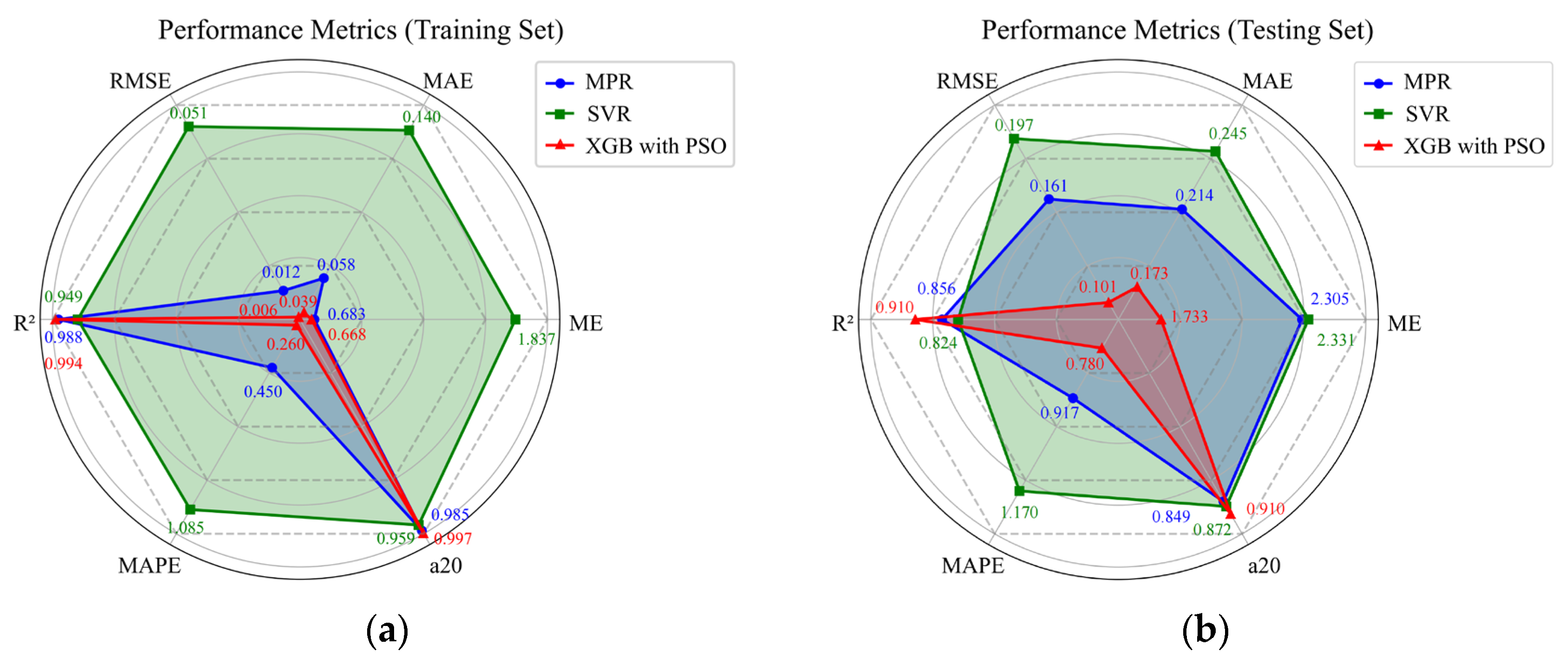
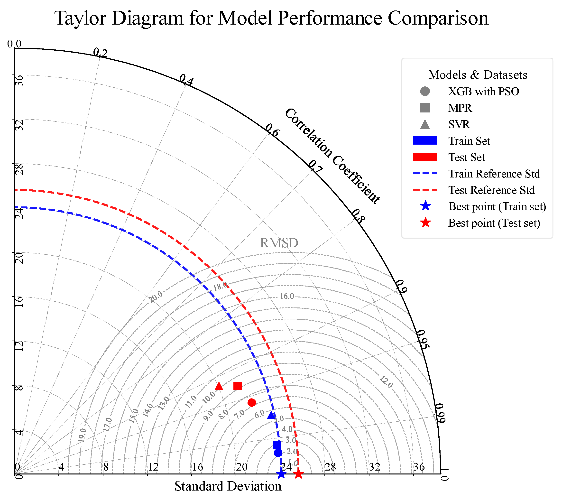
To compare the accuracy differences among traditional regression models, SVR models, and ensemble learning models (optimized by different algorithms) in the task of predicting the compressive strength of CNT-reinforced concrete, this study selected the best-performing representatives from the traditional regression and ensemble learning categories. For traditional regression, the MPR model was chosen, while for ensemble learning, the XGB model optimized by PSO was selected. Based on the performance of these three model types across various prediction metrics, normalized radar charts were created, as shown in Figure 18. Figure 19 presents the Taylor diagram for the performance evaluation of different learning models.

The XGB model optimized by PSO demonstrated the highest prediction accuracy on both the training and test sets, as shown in Figure 18 and Figure 19. This result fully highlights the significant advantage of ensemble learning models, particularly XGB, in prediction tasks involving tabular data. The MPR model, a traditional regression method, performed well on the training set, but its predictive performance on the test set dropped significantly, indicating a certain risk of overfitting. Nevertheless, the MPR model still showed the second-highest prediction accuracy. The performance of the SVR model was inferior to the two aforementioned models. On the test set, its prediction results showed a relatively large MAPE, while the other metrics fell within an acceptable range.

5. Model Interpretability Analysis

5.1. SHapley Additive exPlanations (SHAP) Plots

SHAP is a model explanation method rooted in cooperative game theory. It quantifies the contribution of each feature to a model’s prediction by assigning it a specific importance value, known as the SHAP value. For a given prediction sample x, the SHAP value for feature i, denoted as ${shap}_i\left(x\right)$, is mathematically defined as:

$${shap}_i\left(x\right)=\sum _{S\subseteq F\left\{i\right\}}{\displaystyle \frac{\left|S\right|!\left(\left|F\right|-\left|S\right|-1\right)!}{\left|F\right|!}}\left[f\left(x_S\cup \{i\right\})-f(x_S)\right],$$

(24)

where $F$ is the set of all features. $S$ is any subset of features that does not include feature $i$. $f\left(x_S\right)$ is the model’s prediction using only the features in subset $S$. $\left|F\right|$ is the total number of features.

This formula calculates the marginal contribution of feature $i$ by iterating through all possible feature subsets. It computes the change in the model’s output when feature $i$ is added to each subset and then calculates a weighted average of these contributions. The weighting ensures that the feature attributions satisfy desirable properties, such as symmetry and efficiency, which are grounded in axiomatic principles.

A key advantage of SHAP is its strong theoretical foundation, which guarantees consistency and local accuracy in feature attribution. This allows it to provide comprehensive insights into feature importance. SHAP is highly versatile, applicable not only to SVM, but also to tree-based ensemble models like RF, XGB, and LGBM. Furthermore, SHAP plots offer profound insights into a model’s decision-making process. They not only reveal the magnitude of a feature’s impact on a prediction but also visualize its direction (positive or negative), making the model’s logic more transparent.

5.2. Traditional Regression Models

The primary advantage of traditional regression models lies in their interpretability. Combined with the previous fitting analysis of the compressive strength of CNT-reinforced concrete, the relationship between the target variable and the selected features is better suited to a multivariate polynomial form. The terms output by the MPR model are the products of feature variables (or their interaction combinations) and their corresponding polynomial coefficients. The sign of a coefficient indicates the direction of the effect, while its absolute value represents the magnitude.

By extracting the top ten terms with the largest polynomial coefficients from the MPR model’s output (see

Table 8. Top ten terms with the largest polynomial coefficients from the MPR model output.

Term	Coefficient
age^2*sf_PC^3	−0.074709
age^3*sf_PC^2	0.060474
age^2*sf_PC^2	−0.042611
w/c*CNT_ID*CNT_L*CNT/c^2	0.039527
age^4	−0.038722
CNT_ID*CNT_L*CNT/c^2*sf_PC	−0.037113
CNT_ID^2*CNT_L*CNT/c^2	0.036844
w/c^2*age^2	−0.035781
s/c*age^2*sf_PC^2	0.035533

), key influencing factors can be clearly identified. Age and the surfactant PC are the most critical determinants of compressive strength, followed by the water–cement ratio, mass percentage of CNT to cement, and dimensional parameters of CNT. Specifically, the term CNT_ID*CNT_L*CNT/c^2 shows a positive contribution to compressive strength, whereas sf_PC exhibits a negative effect. These patterns are quantified by the magnitude and sign of the coefficients. Although the MPR model intuitively represents the influence of feature variables on the target variable through a polynomial form, it is still difficult to directly determine the impact of a single feature variable on the target variable.

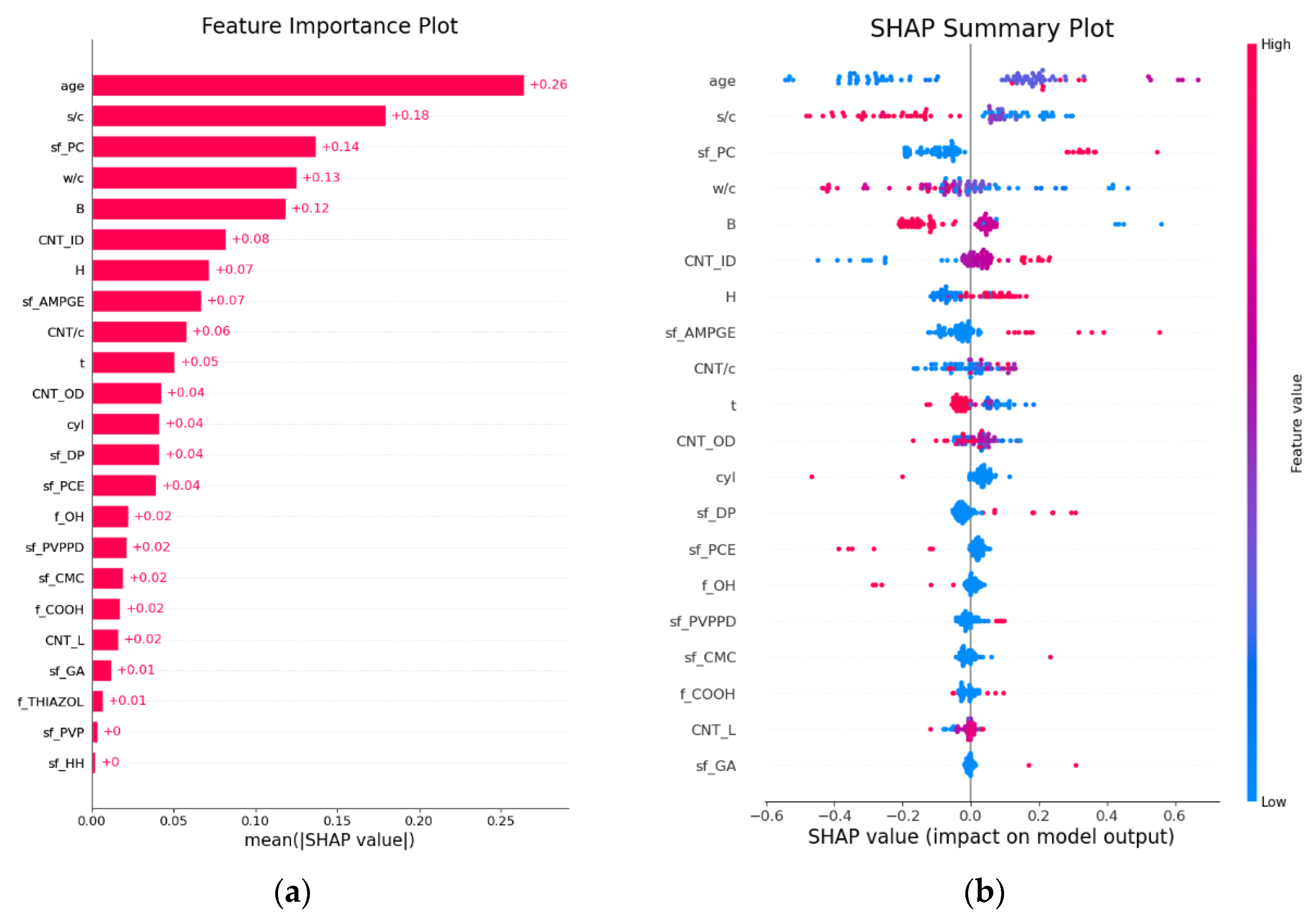
5.3. SVR

Since it is difficult to directly analyze the influence of features on the target variable from the results of an SVR model, this study introduces SHAP plots for model interpretability analysis. Figure 20 presents the feature importance ranking and SHAP values for predictions by the SVR model. In terms of feature importance, the primary factor affecting the compressive strength is age, followed by the sand–cement ratio, surfactant PC, water–cement ratio, and specimen size. A lower curing age (blue dots) has a negative impact on compressive strength, while a higher age (red dots) has a positive impact, reflecting the trend that strength increases with age. The use of surfactant PC enhances compressive strength, whereas increasing the sand–cement ratio, water–cement ratio, or specimen side length or diameter reduces it. It is noteworthy that the CNT parameters (such as CNT inner diameter and CNT outer diameter) did not play a dominant role in influencing compressive strength, and the effects of CNT outer diameter and CNT length were even weaker. The positive effect of the surfactant PC is more prominent in the SVR model, which differs from the MPR model. It indirectly suggests that the SVR model places greater emphasis on the impact of CNT dispersion on compressive strength.

5.4. Ensemble Learning Models

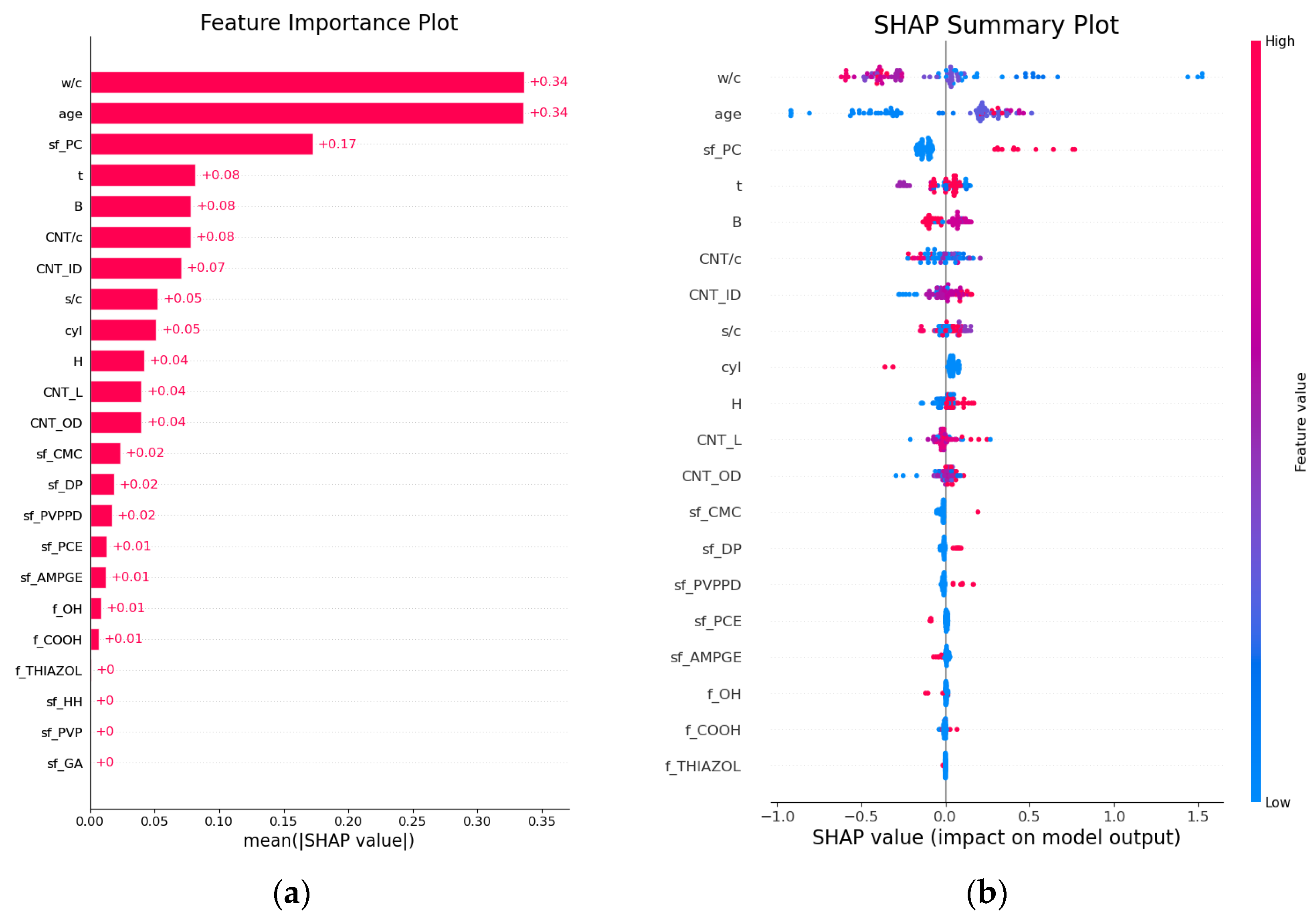
Given that the XGB model optimized by PSO performed the best, it was selected for SHAP analysis. Figure 21 shows the feature importance ranking and SHAP values for the predictions by the PSO-optimized XGB model. In terms of feature importance, the primary factors affecting the compressive strength of CNT-reinforced concrete are the water–cement ratio and age, followed by specimen size, surfactant PC, mass percentage of CNT to cement, and dimensions of CNTs. A lower water–cement ratio (blue dots) has a positive impact on compressive strength, while a higher ratio (red dots) has a negative impact, reflecting the trend that strength decreases as the water–cement ratio increases. The effect of curing age is the opposite. Using surfactant PC or increasing CNT inner diameter both enhance compressive strength. The relationships between mass percentage of CNT to cement, CNT outer diameter, CNT length, sonication duration, and compressive strength are not simple linear ones. For the mass percentage of CNT to cement, both excessively low and high values can lead to a decrease in concrete strength, indicating that there exists an optimal range for a mass percentage of CNT to cement to maximize strength. The specific boundaries of this range will be further analyzed in conjunction with SHAP dependence plots later.

5.5. Weighted Average Importance Analysis of Features

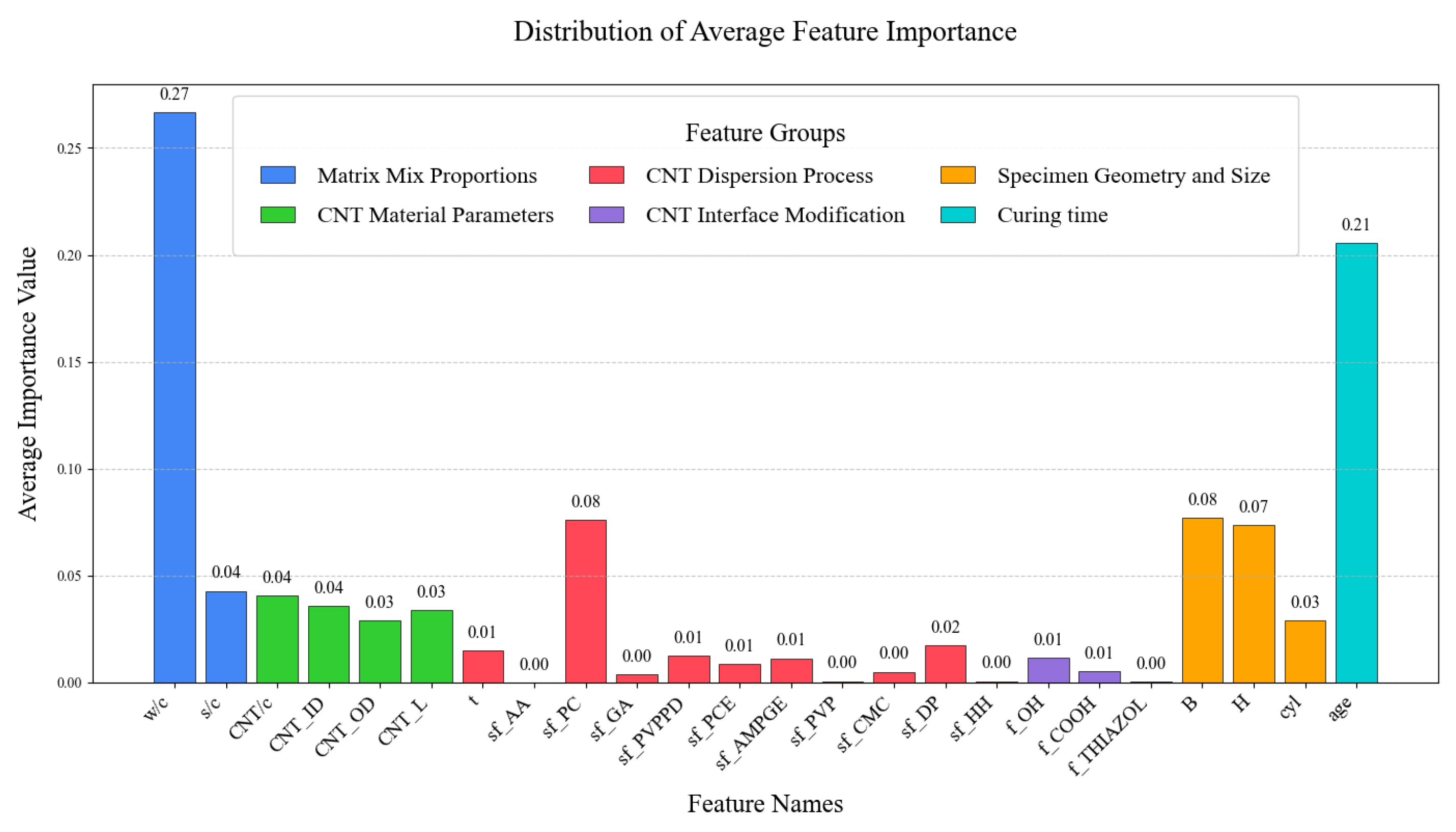
This study analyzed 23 feature variables related to the factors influencing the compressive strength of CNT-reinforced concrete, categorized into six core dimensions: matrix mix proportions, CNT material parameters, dispersion process, interface modification, specimen geometry and size, and curing time. Due to the varying predictive performance of different models, a simple averaging of feature importance from each model would weaken the contribution of high-performance models and fail to accurately reflect the true influence patterns of the features. To more reasonably integrate the feature importance results from multiple models, this study quantifies the weight of each model based on its prediction performance metrics and calculates the weighted average importance of features using Equation (25).

$$\left\{\begin{array}{c}{score}_i={\displaystyle \frac{{R^2}_i}{\sum {R^2}_i}}+{\displaystyle \frac{\frac{1}{{RMSE}_i}}{\sum \left(\frac{1}{{RMSE}_i}\right)}}+{\displaystyle \frac{\frac{1}{{MAE}_i}}{\sum \left(\frac{1}{{MAE}_i}\right)}}+{\displaystyle \frac{\frac{1}{{ME}_i}}{\sum \left(\frac{1}{{ME}_i}\right)}}+{\displaystyle \frac{{a20}_i}{\sum {a20}_i}}+{\displaystyle \frac{\frac{1}{{MAPE}_i}}{\sum \left(\frac{1}{{MAPE}_i}\right)}}\\ {score}_{i,ave}={\displaystyle \frac{{score}_i}{\sum {score}_i}}\\ M_{j,ave}=\sum M_{j,i}\times {score}_{i,ave}\end{array}\right.,$$

(25)

where ${score}_i$ is the score of the i-th model. ${R^2}_i$, ${RMSE}_i$, ${MAE}_i$, ${a20}_i$, and ${MAPE}_i$ are the respective performance metrics for that model. ${score}_{i,ave}$ is the normalized score of the i-th model. $M_{j,i}$ is the importance of the j-th feature in the i-th model. $M_{j,ave}$ is the weighted average importance of the j-th feature.

Figure 22 presents the distribution of the weighted average importance of all features across the different ML models. As shown in the figure, the feature importance for compressive strength in descending order is matrix mix proportions (weighted sum of 0.31), followed by curing time (0.21), then specimen geometry and size (0.18), CNT material parameters (0.14), CNT dispersion process (0.14), and, finally, CNT interface modification (0.02).

(1) Matrix mix proportions. Both the water–cement ratio and sand–cement ratio are key influencing factors, with the influence of w/c significantly greater than that of s/c.

(2) Curing time. Age is a major factor affecting the compressive strength of CNT-reinforced concrete. Apart from the water–cement ratio, its proportion of importance is significantly higher than other features.

(3) Specimen geometry and size. The size and shape of the specimen have a significant impact on the compressive strength and are factors that cannot be ignored.

(4) CNT material parameters. Within this dimension, the mass percentage of CNT to cement and CNT inner diameter have the highest influence, followed by CNT length and CNT outer diameter. In contrast, studies by [36,40,80] found that CNT length had a greater impact. This discrepancy might be because their data sample sizes were insufficient (less than 300), and they used fewer model algorithms. Additionally, references [36,80] did not deeply investigate the effects of the CNT inner diameter and outer diameter.

(5) CNT dispersion process. The effects of different treatment methods vary significantly. The effect of surfactant PC is the most prominent, followed by surfactant DP. The impacts of sonication duration, surfactant PVPPD, PCE, and AMPGE are minimal, while the effects of surfactant AA, GA, PVP, CMC, and HH are negligible.

(6) CNT interface modification. The effect of CNT functional group OH⁻ is the most significant, followed by the functional group COOH⁻ treatment. The impact of other modification methods is negligible.

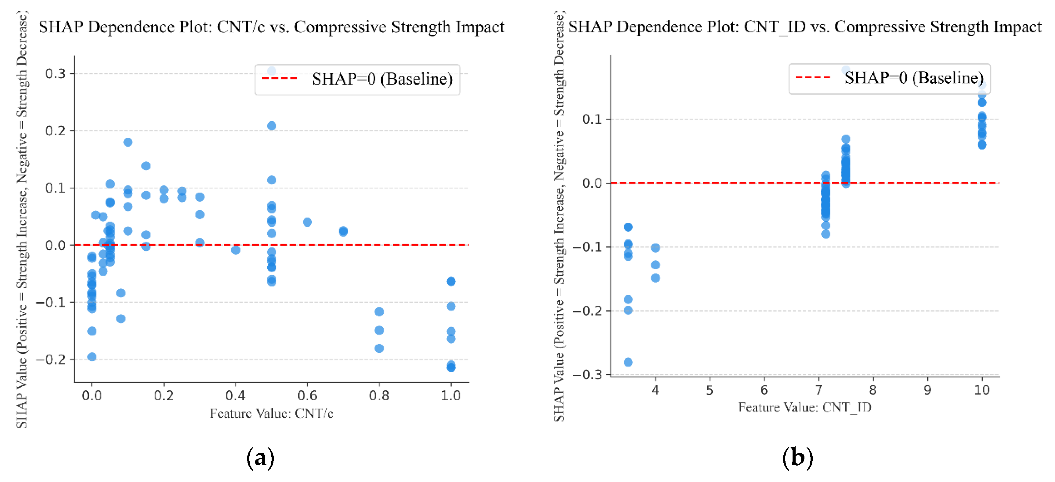
To specifically reveal the influence mechanism of CNT-related features on concrete compressive strength, key features such as the mass percentage of CNT to cement, CNT inner diameter, CNT outer diameter, CNT length, surfactant PC, and functional group OH⁻ were selected to create SHAP dependence plots, as shown in Figure 23. In the plots, the red dashed line represents the baseline where the SHAP value is 0. SHAP values above and below the baseline indicate enhancing and reducing effects on concrete strength, respectively.

(1) The mass percentage of CNT to cement in the range of 0.1–0.3% can increase concrete compressive strength, whereas dosages that are too low or too high lead to a decrease in strength. However, Kumar et al. [14] suggested that a mass percentage of CNT to cement up to 0.5% could enhance compressive strength. The SHAP dependence plot analysis shows that while some samples with CNT/c = 0.5% do exhibit a trend of increased strength, other samples experience a reduction in strength at the same dosage. Considering this variability, to reliably ensure a strength enhancement, this study conservatively suggests a mass percentage of CNT to cement within the 0.1–0.3% range.

(2) Compressive strength gradually increases with a larger CNT inner diameter, and the strength-enhancing effect is only observed when the inner diameter is no less than 7.132 nm. Strength tends to decrease as the CNT outer diameter increases. This is because, for a given mass, smaller-diameter CNTs possess a higher specific surface area, which provides a larger contact interface for bonding with the cement matrix and improves stress transfer [81]. However, except for the extreme case of an 80 nm outer diameter, this feature generally has a positive effect on concrete strength, quantitatively capturing the trade-off between a high surface area and the practical challenges of dispersion [82].

(3) For CNT length, the SHAP dependence plot shows that the commonly used length of around 25 μm actually reduces compressive strength, whereas the length within the 1–15 μm range consistently enhances strength. This is because while longer CNTs theoretically offer better crack-bridging, they are extremely difficult to disperse and tend to form strength-reducing agglomerates [83]. These agglomerates act as defects in the cement matrix, causing a stress concentration that negates any potential reinforcement benefits.

(4) Surfactant PC can consistently enhance the compressive strength, whereas the OH⁻ functional group can significantly reduce the strength. This result is explained by the fact that PC acts as a highly effective superplasticizer, reducing the water–cement ratio and thus densifying the matrix [84]. Conversely, the negative impact of the OH⁻ group, while seemingly counter-intuitive to the goal of improving dispersion, reveals a critical trade-off in practice. The aggressive chemical processes typically used to functionalize CNTs with OH⁻ groups (e.g., strong acid treatment) are known to cause significant structural damage to the nanotubes, creating defects that compromise their intrinsic mechanical properties [85]. These damaged CNTs can then act as stress concentration points within the matrix. Therefore, our model’s findings suggest that, in many practical scenarios, the strength reduction caused by this structural damage may outweigh the potential benefits gained from the improved dispersion.

6. Conclusions

This study systematically compiled 429 sets of experimental data to construct a multi-dimensional database covering 11 core influencing factors, including matrix mix proportions, CNT material characteristics, CNT dispersion processes, CNT interface modifications, specimen geometry and size, and curing time. Based on this database, a systematic training, performance comparison, and evaluation of traditional statistical regression models (MLR, MPR, MARS), a mainstream classical model (SVR), and ensemble learning models (RF, XGB, LGBM) optimized with two hyperparameter tuning methods (PSO and BO) were conducted. The influence of key features on the compressive strength of CNT-reinforced concrete was further analyzed. The conclusions are summarized as the following:

(1) This study successfully established a robust predictive framework for the compressive strength of CNT-reinforced concrete. The PSO-optimized XGB model demonstrated the highest predictive accuracy (test set R² = 0.910). The investigation of hyperparameter optimization methods revealed that PSO achieves superior accuracy at a higher computational cost, while BO provides greater efficiency.

(2) While confirming the foundational impact of matrix mix proportions and curing age, this study’s primary contribution is the quantitative analysis of CNT-related parameters. Among these, CNT mass ratio and inner diameter were identified as the most critical factors influencing strength, with their importance surpassing that of CNT length and outer diameter. Furthermore, the dispersion process, particularly the use of PC surfactant, proved to be a more significant contributor than the CNT’s surface functional group.

(3) Guidelines for optimizing the use of CNTs in concrete are provided. To achieve strength enhancement, the results suggest an optimal CNT mass ratio of 0.1–0.3%, a length of 1–15 μm, and an inner diameter ≥ 7.132 nm. The use of PC surfactant is consistently beneficial, whereas OH⁻ functionalization is shown to be detrimental to compressive strength.

References

1. Ateş, A. Mechanical Properties of Sandy Soils Reinforced with Cement and Randomly Distributed Glass Fibers (GRC). Compos. Part B Eng. 2016, 96, 295–304. [Google Scholar] [CrossRef]
2. Hambach, M.; Möller, H.; Neumann, T.; Volkmer, D. Carbon Fibre Reinforced Cement-Based Composites as Smart Floor Heating Materials. Compos. Part B Eng. 2016, 90, 465–470. [Google Scholar] [CrossRef]
3. Shah, S.P.; Ouyang, C. Mechanical Behavior of Fiber-Reinforced Cement-Based Composites. J. Am. Ceram. Soc. 1991, 74, 2727–2953. [Google Scholar] [CrossRef]
4. Wang, J.-Y.; Banthia, N.; Zhang, M.-H. Effect of Shrinkage Reducing Admixture on Flexural Behaviors of Fiber Reinforced Cementitious Composites. Cem. Concr. Compos. 2012, 34, 443–450. [Google Scholar] [CrossRef]
5. Topçu, İ.B.; Canbaz, M. Effect of Different Fibers on the Mechanical Properties of Concrete Containing Fly Ash. Constr. Build. Mater. 2007, 21, 1486–1491. [Google Scholar] [CrossRef]
6. Yoo, D.-Y.; Shin, H.-O.; Yang, J.-M.; Yoon, Y.-S. Material and Bond Properties of Ultra High Performance Fiber Reinforced Concrete with Micro Steel Fibers. Compos. Part B Eng. 2014, 58, 122–133. [Google Scholar] [CrossRef]
7. Hsu, T.T.C.; Slate, F.O.; Sturman, G.M.; Winter, G. Microcracking of Plain Concrete and the Shape of the Stress-Strain Curve. ACI J. Proc. 1963, 60, 209–224. [Google Scholar] [CrossRef]
8. Jiang, S.; Zhou, D.; Zhang, L.; Ouyang, J.; Yu, X.; Cui, X.; Han, B. Comparison of Compressive Strength and Electrical Resistivity of Cementitious Composites with Different Nano- and Micro-Fillers. Arch. Civ. Mech. Eng. 2018, 18, 60–68. [Google Scholar] [CrossRef]
9. Kaushik, B.K.; Goel, S.; Rauthan, G. Future VLSI Interconnects: Optical Fiber or Carbon Nanotube—A Review. Microelectron. Int. 2007, 24, 53–63. [Google Scholar] [CrossRef]
10. Yu, M.-F.; Lourie, O.; Dyer, M.J.; Moloni, K.; Kelly, T.F.; Ruoff, R.S. Strength and Breaking Mechanism of Multiwalled Carbon Nanotubes Under Tensile Load. Science 2000, 287, 637–640. [Google Scholar] [CrossRef] [PubMed]
11. Walters, D.A.; Ericson, L.M.; Casavant, M.J.; Liu, J.; Colbert, D.T.; Smith, K.A.; Smalley, R.E. Elastic Strain of Freely Suspended Single-Wall Carbon Nanotube Ropes. Appl. Phys. Lett. 1999, 74, 3803–3805. [Google Scholar] [CrossRef]
12. Lu, Z.; Hou, D.; Meng, L.; Sun, G.; Lu, C.; Li, Z. Mechanism of Cement Paste Reinforced by Graphene Oxide/Carbon Nanotubes Composites with Enhanced Mechanical Properties. RSC Adv. 2015, 5, 100598–100605. [Google Scholar] [CrossRef]
13. Parveen, S.; Rana, S.; Fangueiro, R. A Review on Nanomaterial Dispersion, Microstructure, and Mechanical Properties of Carbon Nanotube and Nanofiber Reinforced Cementitious Composites. J. Nanomater. 2013, 2013, 710175. [Google Scholar] [CrossRef]
14. Kumar, S.; Kolay, P.; Malla, S.; Mishra, S. Effect of Multi-Walled Carbon Nano Tubes (CNT) on Mechanical Strength of Cement Paste. J. Mater. Civ. Eng. 2012, 24, 84. [Google Scholar] [CrossRef]
15. Chaipanich, A.; Rianyoi, R.; Nochaiya, T. The Effect of Carbon Nanotubes and Silica Fume on Compressive Strength and Flexural Strength of Cement Mortars. Mater. Today Proc. 2017, 4, 6065–6071. [Google Scholar] [CrossRef]
16. Gillani, S.S.-H.; Khitab, A.; Ahmad, S.; Khushnood, R.A.; Ferro, G.A.; Saleem Kazmi, S.M.; Qureshi, L.A.; Restuccia, L. Improving the Mechanical Performance of Cement Composites by Carbon Nanotubes Addition. Procedia Struct. Integr. 2017, 3, 11–17. [Google Scholar] [CrossRef]
17. Xu, S.; Liu, J.; Li, Q. Mechanical Properties and Microstructure of Multi-Walled Carbon Nanotube-Reinforced Cement Paste. Constr. Build. Mater. 2015, 76, 16–23. [Google Scholar] [CrossRef]
18. Wang, B.; Han, Y.; Liu, S. Effect of Highly Dispersed Carbon Nanotubes on the Flexural Toughness of Cement-Based Composites. Constr. Build. Mater. 2013, 46, 8–12. [Google Scholar] [CrossRef]
19. Nataraja, M.C.; Dhang, N.; Gupta, A.P. Statistical Variations in Impact Resistance of Steel Fiber-Reinforced Concrete Subjected to Drop Weight Test. Cem. Concr. Res. 1999, 29, 989–995. [Google Scholar] [CrossRef]
20. Nili, M.; Afroughsabet, V. Combined Effect of Silica Fume and Steel Fibers on the Impact Resistance and Mechanical Properties of Concrete. Int. J. Impact Eng. 2010, 37, 879–886. [Google Scholar] [CrossRef]
21. Song, P.S.; Wu, J.C.; Hwang, S.; Sheu, B.C. Assessment of Statistical Variations in Impact Resistance of High-Strength Concrete and High-Strength Steel Fiber-Reinforced Concrete. Cem. Concr. Res. 2005, 35, 393–399. [Google Scholar] [CrossRef]
22. Shirkouh, A.H.; Soliman, A. Rubberized Alkali-Activated Concrete—A Review. In Proceedings of the Canadian Society of Civil Engineering Annual Conference 2021, Niagara Falls, ON, Canada, 26–29 May 2021; Walbridge, S., Nik-Bakht, M., Ng, K.T.W., Shome, M., Alam, M.S., el Damatty, A., Lovegrove, G., Eds.; Springer Nature: Singapore, 2023; pp. 561–570. [Google Scholar]
23. Feng, D.-C.; Li, J. Stochastic Nonlinear Behavior of Reinforced Concrete Frames. II: Numerical Simulation. J. Struct. Eng. 2016, 142, 04015163. [Google Scholar] [CrossRef]
24. Feng, D.; Ren, X.; Li, J. Stochastic Damage Hysteretic Model for Concrete Based on Micromechanical Approach. Int. J. Non-Linear Mech. 2016, 83, 15–25. [Google Scholar] [CrossRef]
25. Chopra, P.; Sharma, R.K.; Kumar, M.; Chopra, T. Comparison of Machine Learning Techniques for the Prediction of Compressive Strength of Concrete. Adv. Civ. Eng. 2018, 2018, 5481705. [Google Scholar] [CrossRef]
26. Oliver, J.; Huespe, A.E.; Samaniego, E.; Chaves, E.W.V. Continuum Approach to the Numerical Simulation of Material Failure in Concrete. Int. J. Numer. Anal. Methods Geomech. 2004, 28, 609–632. [Google Scholar] [CrossRef]
27. Feng, D.-C.; Xie, S.-C.; Deng, W.-N.; Ding, Z.-D. Probabilistic Failure Analysis of Reinforced Concrete Beam-Column Sub-Assemblage under Column Removal Scenario. Eng. Fail. Anal. 2019, 100, 381–392. [Google Scholar] [CrossRef]
28. Feng, D.-C.; Wang, Z.; Wu, G. Progressive Collapse Performance Analysis of Precast Reinforced Concrete Structures. Struct. Des. Tall Spec. Build. 2019, 28, e1588. [Google Scholar] [CrossRef]
29. Lu, P.; Chen, S.; Zheng, Y. Artificial Intelligence in Civil Engineering. Math. Probl. Eng. 2012, 2012, 145974. [Google Scholar] [CrossRef]
30. Ley, C.; Bordas, S.P.A. What Makes Data Science Different? A Discussion Involving Statistics2.0 and Computational Sciences. Int. J. Data Sci. Anal. 2018, 6, 167–175. [Google Scholar] [CrossRef]
31. Salehi, H.; Burgueño, R. Emerging Artificial Intelligence Methods in Structural Engineering. Eng. Struct. 2018, 171, 170–189. [Google Scholar] [CrossRef]
32. Nazar, S.; Yang, J.; Amin, M.N.; Khan, K.; Javed, M.F.; Althoey, F. Formulation of Estimation Models for the Compressive Strength of Concrete Mixed with Nanosilica and Carbon Nanotubes. Dev. Built Environ. 2023, 13, 100113. [Google Scholar] [CrossRef]
33. Jiao, H.; Wang, Y.; Li, L.; Arif, K.; Farooq, F.; Alaskar, A. A Novel Approach in Forecasting Compressive Strength of Concrete with Carbon Nanotubes as Nanomaterials. Mater. Today Commun. 2023, 35, 106335. [Google Scholar] [CrossRef]
34. Huang, J.S.; Liew, J.X.; Liew, K.M. Data-Driven Machine Learning Approach for Exploring and Assessing Mechanical Properties of Carbon Nanotube-Reinforced Cement Composites. Compos. Struct. 2021, 267, 113917. [Google Scholar] [CrossRef]
35. Adel, H.; Palizban, S.M.M.; Sharifi, S.S.; Ilchi Ghazaan, M.; Habibnejad Korayem, A. Predicting Mechanical Properties of Carbon Nanotube-Reinforced Cementitious Nanocomposites Using Interpretable Ensemble Learning Models. Constr. Build. Mater. 2022, 354, 129209. [Google Scholar] [CrossRef]
36. Yang, J.; Fan, Y.; Zhu, F.; Ni, Z.; Wan, X.; Feng, C.; Yang, J. Machine Learning Prediction of 28-Day Compressive Strength of CNT/Cement Composites with Considering Size Effects. Compos. Struct. 2023, 308, 116713. [Google Scholar] [CrossRef]
37. Yang, D.; Xu, P.; Zaman, A.; Alomayri, T.; Houda, M.; Alaskar, A.; Javed, M.F. Compressive Strength Prediction of Concrete Blended with Carbon Nanotubes Using Gene Expression Programming and Random Forest: Hyper-Tuning and Optimization. J. Mater. Res. Technol. 2023, 24, 7198–7218. [Google Scholar] [CrossRef]
38. Li, Y.; Li, H.; Jin, C.; Shen, J. The Study of Effect of Carbon Nanotubes on the Compressive Strength of Cement-Based Materials Based on Machine Learning. Constr. Build. Mater. 2022, 358, 129435. [Google Scholar] [CrossRef]
39. Li, T.; Yang, J.; Jiang, P.; Abuhussain, M.A.; Zaman, A.; Fawad, M.; Farooq, F. Forecasting the Strength of Nanocomposite Concrete Containing Carbon Nanotubes by Interpretable Machine Learning Approaches with Graphical User Interface. Structures 2024, 59, 105821. [Google Scholar] [CrossRef]
40. Manan, A.; Zhang, P.; Ahmad, S.; Umar, M.; Raza, A. Machine Learning Prediction Model Integrating Experimental Study for Compressive Strength of Carbon-Nanotubes Composites. J. Eng. Res. 2024, 13, 2193–2211. [Google Scholar] [CrossRef]
41. Osborne, J.W.; Waters, E. Four assumptions of multiple regression that researchers should always test. Pract. Assess. Res. Eval. 2002, 8, 2. [Google Scholar] [CrossRef]
42. Bradley, R.A.; Srivastava, S.S. Correlation in Polynomial Regression. Am. Stat. 1979, 33, 11–14. [Google Scholar] [CrossRef]
43. Khalaf, G.; Shukur, G. Choosing Ridge Parameter for Regression Problems. Commun. Stat. Theory Methods 2005, 34, 1177–1182. [Google Scholar] [CrossRef]
44. Stone, M.H. The Generalized Weierstrass Approximation Theorem. Math. Mag. 1948, 21, 237–254. [Google Scholar] [CrossRef]
45. Friedman, J.H. Multivariate Adaptive Regression Splines. Ann. Stat. 1991, 19, 1–67. [Google Scholar] [CrossRef]
46. De Veaux, R.D.; Psichogios, D.C.; Ungar, L.H. A Comparison of Two Nonparametric Estimation Schemes: MARS and Neural Networks. Comput. Chem. Eng. 1993, 17, 819–837. [Google Scholar] [CrossRef]
47. Craven, P.; Wahba, G. Smoothing Noisy Data with Spline Functions. Numer. Math. 1978, 31, 377–403. [Google Scholar] [CrossRef]
48. Vapnik, V.N. The Nature of Statistical Learning Theory; Springer: New York, NY, USA, 2000; ISBN 978-1-4419-3160-3. [Google Scholar]
49. Keerthi, S.S.; Lin, C.-J. Asymptotic Behaviors of Support Vector Machines with Gaussian Kernel. Neural Comput. 2003, 15, 1667–1689. [Google Scholar] [CrossRef]
50. Lin, H.-T.; Lin, C.-J. A Study on Sigmoid Kernels for SVM and the Training of Non-PSD Kernels by SMO-Type Methods. Neural Comput. 2003, 3, 16. [Google Scholar]
51. Zhu, X.; Zhang, S.; Jin, Z.; Zhang, Z.; Xu, Z. Missing Value Estimation for Mixed-Attribute Data Sets. IEEE Trans. Knowl. Data Eng. 2011, 23, 110–121. [Google Scholar] [CrossRef]
52. Dong, X.; Yu, Z.; Cao, W.; Shi, Y.; Ma, Q. A Survey on Ensemble Learning. Front. Comput. Sci. 2020, 14, 241–258. [Google Scholar] [CrossRef]
53. Mai, H.-V.T.; Nguyen, M.H.; Trinh, S.H.; Ly, H.-B. Toward Improved Prediction of Recycled Brick Aggregate Concrete Compressive Strength by Designing Ensemble Machine Learning Models. Constr. Build. Mater. 2023, 369, 130613. [Google Scholar] [CrossRef]
54. Breiman, L. Random Forests. Mach. Learn. 2001, 45, 5–32. [Google Scholar] [CrossRef]
55. Chen, T.; Guestrin, C. XGBoost: A Scalable Tree Boosting System. In Proceedings of the 22nd ACM SIGKDD International Conference on Knowledge Discovery and Data Mining, San Francisco, CA, USA, 13–17 August 2016; Association for Computing Machinery: New York, NY, USA, 2016; pp. 785–794. [Google Scholar]
56. Ju, Y.; Sun, G.; Chen, Q.; Zhang, M.; Zhu, H.; Rehman, M.U. A Model Combining Convolutional Neural Network and LightGBM Algorithm for Ultra-Short-Term Wind Power Forecasting. IEEE Access 2019, 7, 28309–28318. [Google Scholar] [CrossRef]
57. Bergstra, J.; Bengio, Y. Random Search for Hyper-Parameter Optimization. J. Mach. Learn. Res. 2012, 13, 281–305. [Google Scholar]
58. Snoek, J.; Larochelle, H.; Adams, R.P. Practical Bayesian Optimization of Machine Learning Algorithms. In Proceedings of the 26th International Conference on Neural Information Processing Systems—Volume 2; Curran Associates Inc.: Red Hook, NY, USA, 2012; Volume 2, pp. 2951–2959. [Google Scholar]
59. Kennedy, J. Particle Swarm Optimization. In Encyclopedia of Machine Learning; Sammut, C., Webb, G.I., Eds.; Springer: Boston, MA, USA, 2010; pp. 760–766. ISBN 978-0-387-30164-8. [Google Scholar]
60. Liu, Y.; Qiu, T.; Hu, H.; Kong, C.; Zhang, Y.; Wang, T.; Zhou, J.; Zou, J. Machine Learning Models for Prediction of Severe Pneumocystis Carinii Pneumonia after Kidney Transplantation: A Single-Center Retrospective Study. Diagnostics 2023, 13, 2735. [Google Scholar] [CrossRef]
61. Pelikan, M. Bayesian Optimization Algorithm. In Hierarchical Bayesian Optimization Algorithm; Studies in Fuzziness and Soft Computing; Springer: Berlin/Heidelberg, Germany, 2005; Volume 170, pp. 31–48. ISBN 978-3-540-23774-7. [Google Scholar]
62. Yu, J.-C.; Ni, K.; Chen, C.-T. ENCAP: Computational Prediction of Tumor T Cell Antigens with Ensemble Classifiers and Diverse Sequence Features. PLoS ONE 2024, 19, e0307176. [Google Scholar] [CrossRef]
63. Brochu, E.; Cora, M.; de Freitas, N. A Tutorial on Bayesian Optimization of Expensive Cost Functions, with Application to Active User Modeling and Hierarchical Reinforcement Learning. arXiv 2010, arXiv:1012.2599. [Google Scholar] [CrossRef]
64. Kohavi, R. A Study of Cross-Validation and Bootstrap for Accuracy Estimation and Model Selection. In Proceedings of the 14th International Joint Conference on Artificial Intelligence—Volume 2; Morgan Kaufmann Publishers Inc.: San Francisco, CA, USA, 1995; Volume 2, pp. 1137–1143. [Google Scholar]
65. Picard, R.R.; Cook, R.D. Cross-Validation of Regression Models. J. Am. Stat. Assoc. 1984, 79, 575–583. [Google Scholar] [CrossRef]
66. Siddique, R.; Aggarwal, P.; Aggarwal, Y. Prediction of Compressive Strength of Self-Compacting Concrete Containing Bottom Ash Using Artificial Neural Networks. Adv. Eng. Softw. 2011, 42, 780–786. [Google Scholar] [CrossRef]
67. Cheng, M.-Y.; Prayogo, D.; Wu, Y.-W. Novel Genetic Algorithm-Based Evolutionary Support Vector Machine for Optimizing High-Performance Concrete Mixture. J. Comput. Civ. Eng. 2014, 28, 06014003. [Google Scholar] [CrossRef]
68. Bui, D.-K.; Nguyen, T.; Chou, J.-S.; Nguyen-Xuan, H.; Ngo, T.D. A Modified Firefly Algorithm-Artificial Neural Network Expert System for Predicting Compressive and Tensile Strength of High-Performance Concrete. Constr. Build. Mater. 2018, 180, 320–333. [Google Scholar] [CrossRef]
69. Omran, B.A.; Chen, Q.; Jin, R. Comparison of Data Mining Techniques for Predicting Compressive Strength of Environmentally Friendly Concrete. J. Comput. Civ. Eng. 2016, 30, 04016029. [Google Scholar] [CrossRef]
70. Tayfur, G.; Erdem, T.K.; Kırca, Ö. Strength Prediction of High-Strength Concrete by Fuzzy Logic and Artificial Neural Networks. J. Mater. Civ. Eng. 2014, 26, 04014079. [Google Scholar] [CrossRef]
71. Chou, J.-S.; Pham, A.-D. Enhanced Artificial Intelligence for Ensemble Approach to Predicting High Performance Concrete Compressive Strength. Constr. Build. Mater. 2013, 49, 554–563. [Google Scholar] [CrossRef]
72. Armaghani, D.J.; Mohamad, E.T.; Narayanasamy, M.S.; Narita, N.; Yagiz, S. Development of Hybrid Intelligent Models for Predicting TBM Penetration Rate in Hard Rock Condition. Tunn. Undergr. Space Technol. 2017, 63, 29–43. [Google Scholar] [CrossRef]
73. Duan, J.; Asteris, P.G.; Nguyen, H.; Bui, X.-N.; Moayedi, H. A Novel Artificial Intelligence Technique to Predict Compressive Strength of Recycled Aggregate Concrete Using ICA-XGBoost Model. Eng. Comput. 2021, 37, 3329–3346. [Google Scholar] [CrossRef]
74. Chen, H.; Asteris, P.; Jahed Armaghani, D.; Gordan, B.; Pham, B. Assessing Dynamic Conditions of the Retaining Wall: Developing Two Hybrid Intelligent Models. Appl. Sci. 2019, 9, 1042. [Google Scholar] [CrossRef]
75. Apostolopoulou, M.; Armaghani, D.J.; Bakolas, A.; Douvika, M.G.; Moropoulou, A.; Asteris, P.G. Compressive Strength of Natural Hydraulic Lime Mortars Using Soft Computing Techniques. Procedia Struct. Integr. 2019, 17, 914–923. [Google Scholar] [CrossRef]
76. Cook, D.J.; Mulrow, C.D.; Haynes, R.B. Systematic Reviews: Synthesis of Best Evidence for Clinical Decisions. Ann. Intern. Med. 1997, 126, 376–380. [Google Scholar] [CrossRef]
77. Windle, P.E. The Systematic Review Process: An Overview. J. PeriAnesthesia Nurs. 2010, 25, 40–42. [Google Scholar] [CrossRef] [PubMed]
78. Arlot, S.; Celisse, A. A Survey of Cross-Validation Procedures for Model Selection. Stat. Surv. 2010, 4, 40–79. [Google Scholar] [CrossRef]
79. Gesoğlu, M.; Güneyisi, E.; Özbay, E. Properties of Self-Compacting Concretes Made with Binary, Ternary, and Quaternary Cementitious Blends of Fly Ash, Blast Furnace Slag, and Silica Fume. Constr. Build. Mater. 2009, 23, 1847–1854. [Google Scholar] [CrossRef]
80. Xu, H.; He, Z.; Li, J.; Zhou, S. Multidimensional Transport Experiment and Simulation of Chloride Ions in Concrete Subject to Simulated Dry and Wet Cycles in a Marine Environment. Materials 2023, 16, 7185. [Google Scholar] [CrossRef] [PubMed]
81. Konsta-Gdoutos, M.S.; Metaxa, Z.S.; Shah, S.P. Highly Dispersed Carbon Nanotube Reinforced Cement Based Materials. Cem. Concr. Res. 2010, 40, 1052–1059. [Google Scholar] [CrossRef]
82. Makar, J.M.; Chan, G.W. Growth of Cement Hydration Products on Single-Walled Carbon Nanotubes. J. Am. Ceram. Soc. 2009, 92, 1303–1310. [Google Scholar] [CrossRef]
83. Sobolkina, A.; Mechtcherine, V.; Khavrus, V.; Maier, D.; Mende, M.; Ritschel, M.; Leonhardt, A. Dispersion of Carbon Nanotubes and Its Influence on the Mechanical Properties of the Cement Matrix. Cem. Concr. Compos. 2012, 34, 1104–1113. [Google Scholar] [CrossRef]
84. Plank, J.; Sakai, E.; Miao, C.W.; Yu, C.; Hong, J.X. Chemical Admixtures—Chemistry, Applications and Their Impact on Concrete Microstructure and Durability. Cem. Concr. Res. 2015, 78, 81–99. [Google Scholar] [CrossRef]
85. Datsyuk, V.; Kalyva, M.; Papagelis, K.; Parthenios, J.; Tasis, D.; Siokou, A.; Kallitsis, I.; Galiotis, C. Chemical Oxidation of Multiwalled Carbon Nanotubes. Carbon 2008, 46, 833–840. [Google Scholar] [CrossRef]
Figure 1. Flowchart of the research methodology.
Buildings 15 04349 g001
Figure 2. Fundamental concepts of SVM and SVR: (a) SVM; (b) SVR.
Buildings 15 04349 g002
Figure 3. The kernel function in SVM.
Buildings 15 04349 g003
Figure 4. The fundamental principle of RF.
Buildings 15 04349 g004
Figure 5. Fold cross-validation.
Buildings 15 04349 g005
Figure 6. The distribution characteristics of the feature variables: (a) w/c; (b) s/c; (c) CNT_ID; (d) CNT_OD; (e) CNT_L; (f) CNT/c; (g) sf; (h) f; (i) t; (j) size; (k) age; (l) fc.
Buildings 15 04349 g006aBuildings 15 04349 g006b
Figure 7. Correlation matrix of the dataset.
Buildings 15 04349 g007
Figure 8. Fitting plot results for traditional regression models: (a) MLR; (b) MPR; (c) MARS.
Buildings 15 04349 g008
Figure 9. Normalized radar charts of performance metrics for traditional regression models: (a) training set; (b) test set.
Buildings 15 04349 g009
Figure 10. Taylor diagram for traditional regression models.
Buildings 15 04349 g010
Figure 11. Grid search results for SVR hyperparameters (gamma corresponds to the hyperparameter γ ).
Buildings 15 04349 g011
Figure 12. Fitting plot results of the SVR model after hyperparameter tuning.
Buildings 15 04349 g012
Figure 13. The optimization process for selected hyperparameters in ensemble learning models: (a) n_estimators in RF using PSO; (b) n_estimators in RF using BO; (c) colsample_bytree in XGB using PSO; (d) colsample_bytree in XGB using BO; (e) min_child_weight in LGBM using PSO; (f) min_child_weight in LGBM using BO.
Buildings 15 04349 g013aBuildings 15 04349 g013b
Figure 14. Comparison of validation set R2 and computation time for different models and optimization algorithms.
Buildings 15 04349 g014
Figure 15. Fitting plot results of ensemble learning models after hyperparameter optimization: (a) RF using PSO; (b) RF using BO; (c) XGB using PSO; (d) XGB using BO; (e) LGBM using PSO; (f) LGBM using BO.
Buildings 15 04349 g015aBuildings 15 04349 g015b
Figure 16. Normalized radar charts of performance metrics for the three ensemble learning models under different optimization algorithms: (a) training set; (b) test set.
Buildings 15 04349 g016
Figure 17. Taylor diagram for ensemble learning models.
Buildings 15 04349 g017
Figure 18. Normalized radar charts of performance metrics for different learning models: (a) training set; (b) test set.
Buildings 15 04349 g018
Figure 19. Taylor diagram for different learning models.
Buildings 15 04349 g019
Figure 20. SHAP summary plot and feature importance plot of SVR: (a) feature importance plot; (b) SHAP summary plot.
Buildings 15 04349 g020
Figure 21. SHAP summary plot and feature importance plot of XGB using PSO: (a) feature importance plot; (b) SHAP summary plot.
Buildings 15 04349 g021
Figure 22. Distribution of average feature importance.
Buildings 15 04349 g022
Figure 23. SHAP dependence plots of CNT-related features: (a) CNT/c; (b) CNT_ID; (c) CNT_OD; (d) CNT_L; (e) sf_PC; (f) f_OH.
Buildings 15 04349 g023aBuildings 15 04349 g023b