A High-Dimensional Parameter Identification Method for Pipelines Based on Static Strain and DNN Surrogate Models to Accelerate Langevin Bayesian Inference

Abstract

This study develops a Bayesian parameter identification framework that uses static strain measurements to update pipeline structural models under complex boundary conditions. Because strain responses are directly linked to internal stress states and are much less sensitive to boundary condition uncertainty, the proposed approach retains high identification accuracy where conventional methods based on static displacements or modal data are difficult to apply. The method employs the Metropolis-Adjusted Langevin Algorithm (MALA), a gradient-based MCMC scheme with a Metropolis correction that ensures asymptotically exact sampling, to handle the high dimensional parameter space, and integrates a deep neural network (DNN) surrogate model to accelerate sampling. A numerical example demonstrates the efficiency of MALA in high dimensional settings by exploiting the gradient of the log posterior to guide proposals, successfully identifying the stiffness of 30 pipeline segments and showing that combining axial and hoop direction strain data yields more accurate estimates. An experimental case on a real pipeline corroborates the effectiveness of the approach, reducing the mean absolute error (MAE) of predicted strains from 27.3% to 4.2% after updating. Overall, by coupling MALA with a DNN surrogate, the study establishes a static-strain-based Bayesian inference framework for high dimensional parameter identification in pipelines with complex boundaries, providing a practical route for engineering applications and supporting reliable structural safety assessment.

1. Introduction

Pipeline systems play a critical role in modern industrial and urban infrastructure, extensively applied in the transportation of petroleum, natural gas, chemicals, water, and wastewater. These systems are prevalent in onshore and offshore processing industries, transportation networks, municipal water supply and drainage systems, industrial manufacturing facilities, and power plants. Typically installed underground or underwater, or situated in hard-to-reach areas, pipelines present substantial challenges for inspection and maintenance. Moreover, during prolonged operations, they are vulnerable to fatigue, corrosion, and mechanical damage, leading to significant risks to their structural integrity. Any engineering failure may result in severe environmental pollution, economic loss, and personal injury. Consequently, accurate parameter identification of in-service pipelines has become increasingly important, because accurate knowledge of the structural parameters is decisive for the accuracy of early fault detection and nondestructive evaluation. Therefore, research and technological advancements in pipeline structural parameter identification have emerged as pivotal topics within the engineering and scientific communities, aimed at enhancing the safety and reliability of pipeline systems [1].

One common approach for parameter identification of shell structures, such as pipelines, is the utilization of various electromagnetic signals [1,2] or acoustic signals [3,4]. These techniques prove particularly effective in detecting small-scale defects and do not rely on structural models. However, they typically necessitate the deployment of dense sensor networks and expensive equipment, while also being highly sensitive to noise interference [5,6]. Such stringent requirements render these methods impractical for large-scale structures, especially immovable pipelines that must be tested in situ [7].

Another approach for parameter identification in pipeline structures leverages changes in vibration characteristics. It rests on the premise that corrosion or defects alter mechanical properties, thereby modifying the structure’s dynamic behavior [8]. Such techniques are particularly effective when parameter changes are appreciable or when damage occurs at locations highly sensitive to dynamic responses. However, their sensitivity to small defects is often limited by measurement noise. In addition, the complex boundary conditions of pipelines complicate data acquisition and hamper the formulation of objective functions based on dynamic indicators (e.g., mode shapes).

In the field of pipeline parameter identification, strain-based approaches are more widely used [9]. Numerous studies have developed strain-centric SHM systems using fiber-optic sensors to map the full-field strain distribution along pipelines, thereby enabling parameter identification or qualitative condition assessment. For instance, Kunzler [10] employed multi-axial fiber Bragg grating (FBG) sensors to measure axial and transverse strain fields while investigating the effects of pressure cycling and impact loading. He proposed a method for locating and quantifying fiber breakage and delamination defects and benchmarked it against conventional NDT techniques such as ultrasonic testing and eddy-current inspection. Similarly, Klute [11] embedded a circumferentially wound fiber-optic sensor with a helical pitch along the axis of a composite vessel and used optical frequency-domain reflectometry (OFDR) to obtain strain measurements at multiple positions along the fiber, thereby enabling comprehensive condition monitoring of the vessel.

Zhu [12] employed static strain measurements to automatically evaluate free spans in subsea pipelines. This approach overcomes the limitations of conventional vibration-based methods, which often face difficulties in acquiring reliable vibration data. However, the study was solely based on numerical simulations under idealized environmental conditions, and the practical effectiveness of the method requires further validation in real engineering applications. Zhang [13] utilized full-field strain data obtained via Digital Image Correlation (DIC) to update the force–displacement curve of stainless-steel foil sheets, comparing the results with those from conventional finite element (FE) iterative calibration methods. The study demonstrated the advantages of using strain field data for calibration. Wang [14] applied DIC-derived strain data to update the parameters of Zernike polynomials describing a square plate with a circular hole subjected to uniaxial tensile loading. The updated polynomial model effectively replicated the plate’s full-field response and accurately captured the material’s nonlinear behavior. Zou [15] employed a distributed fiber optic strain and temperature sensor system to identify wall-thinning defects in steel pipes by measuring both axial and tangential strains along the pipeline. This method successfully located and quantified the severity of predefined wall thinning; however, it did not account for measurement variability. Pena [16] monitored complex strain distributions throughout the pressurization process of composite overwrapped pressure vessels (CPVs) using embedded fiber Bragg grating sensors, providing valuable insights into failure mechanisms. Huang [17] proposed a hybrid damage detection method that combines strain monitoring with modal strain curvature node (MSCN) analysis for CPV monitoring, achieving effective damage detection with relatively few sensors. Sotoudehnia [18] employed modal data along with a bi-conjugate gradient method to solve model updating equations for cylindrical shell structures, enabling damage localization and severity assessment even in the presence of noisy data. This study highlighted the pervasive challenge of ill-posedness in parameter identification inverse problems.

To address the challenges of randomness and ill-posedness in pipeline parameter identification, Bayesian methods have been widely adopted. This approach inherently incorporates uncertainties from both the model and measurements, effectively mitigating the ill-posed nature of inverse problems. For example, Gaitanaros [18] utilized strain data within a Bayesian framework to estimate the location, size, and orientation of cracks in structures. The method’s efficacy was demonstrated through simulated data of a single crack in a thin plate subjected to static loading. Additionally, the influence of the number and orientation of strain sensors on crack identification accuracy was investigated. Warner [19] applied a Bayesian Markov Chain Monte Carlo (MCMC) approach, driven by strain data and surrogate models, to identify cracks in fractured plates, overcoming the inherent ill-posedness of crack detection while accounting for measurement uncertainty. Despite these advancements, the number of parameters identifiable through Bayesian approaches remains limited, posing considerable challenges for complex pipeline structures, particularly in scenarios requiring high-dimensional parameter identification to achieve refined model updating.

A common challenge in Bayesian MCMC-based parameter identification is the curse of dimensionality [20,21]. Most algorithms provide reliable inference only when the number of updating parameters is modest; as dimensionality increases, mixing deteriorates and identification quickly becomes impractical. One way to mitigate this is to adopt advanced sampling schemes [22]. Even then, high-dimensional settings typically require many posterior evaluations. For dense finite-element meshes, this necessitates efficient surrogate models to accelerate MCMC. Kriging and response-surface models [23,24], along with their variants, are widely used. With advances in deep learning, neural-network surrogates have also been introduced as drop-in replacements for costly FE analyses; compared with Kriging/RSM, a notable advantage is their natural support for multi-input–multi-output mappings. However, in the specific context of pipeline parameter identification from strain data, the published literature remains limited.

Considering the industrial demand for efficient and fine-grained parameter identification of pipeline structures, this study presents a high dimensional Bayesian MCMC parameter identification method grounded in multi-point strain measurements. The method leverages strain data collected from multiple sensors distributed across various locations and orientations to accurately infer the complex parameters of the pipeline structure. During the identification process, the likelihood function is constructed from the misfit between measured and model predicted strain values (optionally weighted by the measurement-noise covariance). To address the computational challenges posed by high dimensional parameter spaces, we employ a Langevin MCMC sampler that exploits the gradient of the log posterior to guide proposals, together with a multi-input–multi-output (MIMO) deep neural network (DNN) surrogate, which rapidly predicts strains at multiple measurement points and thereby accelerates posterior sampling. Although deep neural network (DNN) surrogates have been successfully applied to a range of engineering inverse problems, including material property identification in composite structures [25] and model updating in fluid-dynamics systems [26], and gradient-based samplers such as the Metropolis-Adjusted Langevin Algorithm (MALA) and Hamiltonian Monte Carlo (HMC) are well established in Bayesian inference [27,28], the integration of a DNN surrogate with a MALA sampler for high-dimensional structural health monitoring has, to the best of our knowledge, not yet been reported. An additional advantage of the Bayesian framework is its ability to explicitly represent and quantify the uncertainties inherent in the pipeline structural model and the stochastic errors in strain measurements, providing a rigorous basis for reliability-oriented engineering decisions.

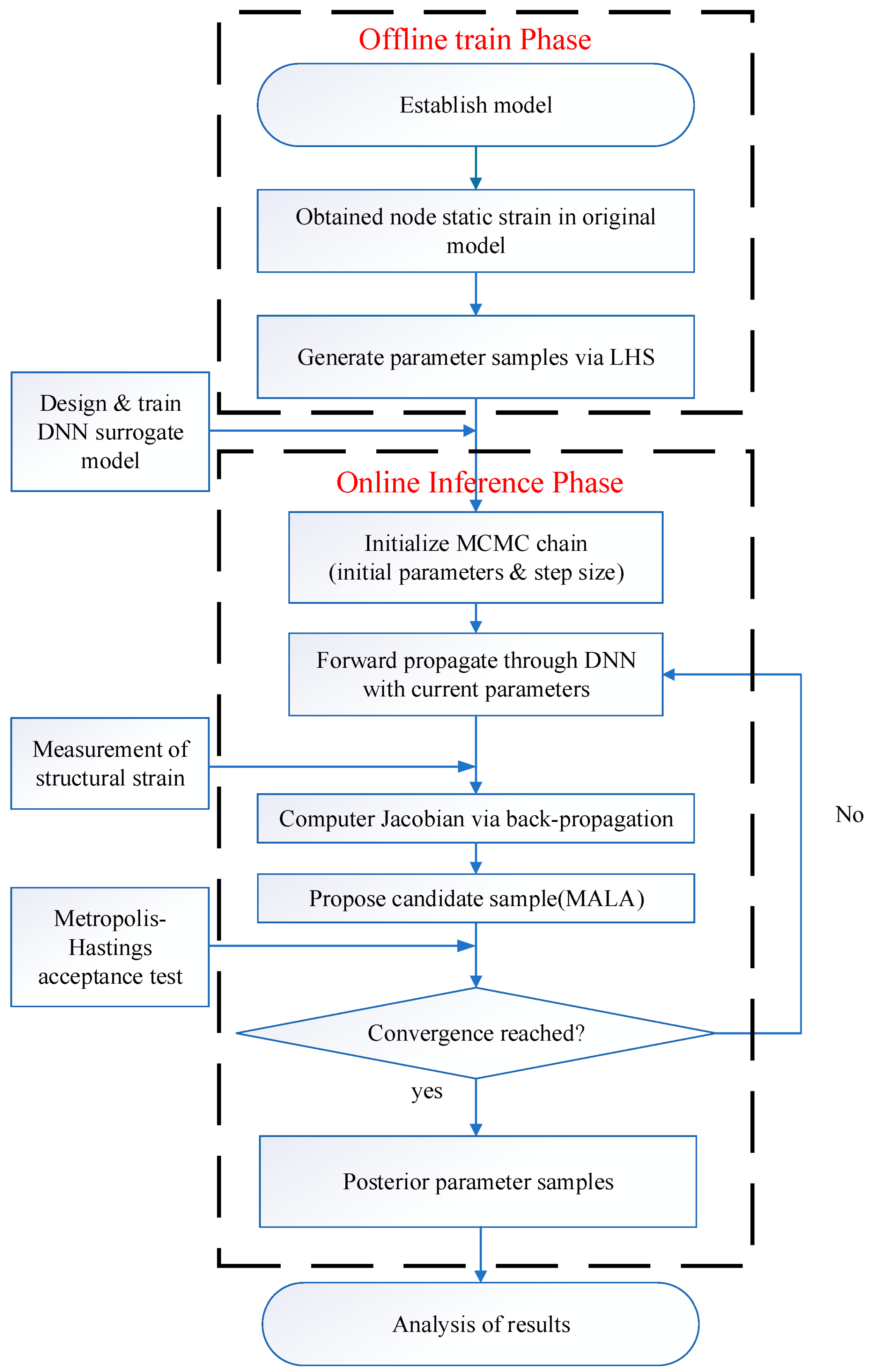
The organization of this paper is as follows: Section 2 introduces the fundamental principles of strain-based Bayesian methods. Section 3 describes the MCMC sampling technique used to obtain the posterior probability density of the parameters to be identified. Section 4 presents the deep neural network (DNN) surrogate model and includes a flowchart illustrating the proposed method. Section 5 shows the efficient Bayesian inference based on DNN Surrogates and Langevin Dynamics. Numerical examples are discussed in Section 6, focusing on the optimal sensor placement strategy and the identification performance for high dimensional parameters. Section 7 reports an experimental case study based on actual measurements, and Section 8 concludes the paper.

2. Review of Basic Principle of Bayesian Parameter Identification

Bayesian methods update the probability distribution of target parameters by combining prior information with observed data to achieve optimal estimation. In structural parameter identification, the Bayesian approach derives the posterior distribution by integrating the prior distribution with the likelihood function. Assuming the current structural parameters are denoted by $\theta$ and the observed data by $D$, according to Bayes’ theorem, the posterior probability density function (PDF) of the structural identification parameters can be expressed as:

$$p\left(\theta /D\right)={\displaystyle \frac{p\left(D/\theta \right)\pi \left(\theta \right)}{p\left(D\right)}}$$

(1)

where $p(D|\theta )$ denotes the likelihood function, representing the probability of observing data $D$ given the structural parameters $\theta$. The likelihood function is defined based on the discrepancy between the observed data and the computed response. $\pi (\theta )$ represents the prior distribution of the structural parameters $\theta$. $p(D)$ is the evidence term, indicating the marginal probability of the observed data $D$, serving as a normalization constant.

When the observed data $D$ corresponds to the structural strain vector $\epsilon$, the likelihood function $p(D|\theta )$ can be expressed as the probability distribution of the difference between the measured and computed strains, which can be formulated as:

$$p\left(\epsilon /\theta \right)={\displaystyle \frac{1}{\sqrt{\left|cov\right|\cdot (2\pi )}}}\cdot \exp \left(-{\displaystyle \frac{1}{2}}{\left(\epsilon -\epsilon (\theta )\right)}^T\cdot co{v}^{-1}\left(\epsilon -\epsilon (\theta )\right)\right)$$

(2)

where $\epsilon$ and $\epsilon (\theta )$ denote the measured and computed strain vectors, respectively. $cov$ represents the covariance matrix of the measurement noise in the strain data, which is typically assumed to be diagonal. Under these assumptions, the posterior PDF of the structural parameters vector $\theta$ based on strain measurements can be written as:

$$p\left(\theta /\epsilon \right)\propto p\left(\epsilon /\theta \right)\pi \left(\theta \right)$$

(3)

Since the posterior distribution $p(\theta |\epsilon )$ typically lacks a closed-form expression, numerical methods are required for its approximation. MCMC methods commonly employed in Bayesian model updating provide an effective numerical simulation technique by constructing a Markov chain to sample the parameter space and thereby approximate the posterior distribution.

3. Efficient Bayesian Inference Based on Langevin Dynamics

Although the Bayesian framework provides a solid theoretical foundation for parameter identification, its practical effectiveness in engineering applications critically depends on efficiently exploring the posterior probability distribution $p(\theta |\epsilon )$. Traditional numerical simulation methods, such as the Metropolis–Hastings algorithm, rely on a random-walk mechanism. Even advanced variants like Delayed Rejection Adaptive Metropolis-MCMC (DRAM-MCMC) improve performance through adaptive step sizes, but the inherent randomness of the search remains unchanged. When applied to complex engineering models, particularly those involving high-dimensional parameter vectors $\theta$, these methods often suffer from the “curse of dimensionality”, leading to low efficiency. In high-dimensional spaces, random search results in highly correlated samples, slow convergence, and may fail to fully capture complex multimodal posterior distributions.

To overcome these limitations, this study adopts a more advanced sampling strategy: the Metropolis-Adjusted Langevin Algorithm (MALA), a key member of the Langevin MCMC (LMCMC) family. Unlike random-walk methods, MALA leverages gradient information of the posterior distribution to guide the sampling process. This transforms the originally blind search into a purposeful and directed exploration, analogous to a particle moving in a potential energy field. The gradient-driven nature of MALA enables the Markov chain to move preferentially toward regions where the probability density increases most rapidly, thereby significantly enhancing sampling efficiency and convergence speed in high-dimensional parameter spaces.

3.1. Mathematical Formulation of the MALA

The core of the MALA is the discrete-time approximation of the Langevin stochastic differential equation (SDE). It constructs a proposal mechanism such that, given the current state k, the next state ${\theta }^{(k+1)}$ is generated from ${\theta }^{(k)}$ according to the following equation:

$${\theta }^{(k+1)}={\theta }^{(k)}+{\displaystyle \frac{{\tau }^2}{2}}{\nabla }_{\theta }\log p({\theta }^{(k)}|\epsilon )+\tau \cdot {\xi }^{(k)}$$

(4)

The update formula consists of two key components:

(1)

Drift Term ${\displaystyle \frac{{\tau }^2}{2}}{\nabla }_{\theta }\log p({\theta }^{(k)}|\epsilon )$: This deterministic component drives the parameter vector ${\theta }^{(k)}$ in the direction of the steepest ascent of the log-posterior density. The step size ${\displaystyle \frac{{\tau }^2}{2}}$ controls the magnitude of this movement.

(2)

Diffusion Term $\tau \cdot {\xi }^{(k)}$: This stochastic component introduces randomness, where ${\xi }^{(k)}$ is a standard normal random vector, i.e., ${\xi }^{(k)}$ ~ N(0, I), with I being the n-dimensional identity matrix. This term ensures that the sampler can escape local probability maxima and explore the entire parameter space.

3.2. Gradient Computation and the Sensitivity Matrix

The efficiency of the MALA directly depends on the accurate and efficient computation of the posterior gradient ${\nabla }_{\theta }\log p({\theta }^{(k)}|\epsilon )$. This gradient can be decomposed into the sum of the likelihood gradient $\nabla \log p(\epsilon \mid {\theta }^{(k)})$ and the prior gradient $\nabla \log p({\theta }^{(k)})$:

$$\nabla \log p({\theta }^{(k)}|\epsilon )=\nabla \log p(\epsilon \mid {\theta }^{(k)})+\nabla \log p({\theta }^{(k)})$$

(5)

Assuming both the likelihood and the prior follow Gaussian distributions, the most computationally intensive and critical component in this calculation is the likelihood gradient. By differentiating the likelihood expression in Equation (3), can obtain:

$$\nabla \log p(\epsilon \mid {\theta }^{(k)})=J_c{({\theta }^{(k)})}^{\mathrm{T}}{\Sigma }^{-1}({\epsilon }_m-{\epsilon }_c({\theta }^{(k)}))$$

(6)

In Equation (6), $J_c({\theta }^{(k)})$ denotes the Jacobian matrix of the model response. In the context of structural parameter identification, this matrix is more intuitively referred to as the sensitivity matrix. Each element ${(J_c)}_{ij}=\partial {({\epsilon }_c)}_i/\partial {\theta }_j$ precisely quantifies the sensitivity of the response at the i-th strain measurement location with respect to variations in the j-th structural parameter (for example, the elastic modulus of the j-th pipeline segment).

The gradient driven by sensitivity information is the core advantage of the MALA method, which acts as a physical “interpreter,” efficiently translating the observed errors in the measurement space (strain residuals ${\epsilon }_m-{\epsilon }_c({\theta }^{(k)})$) into a targeted correction vector in the parameter space. This mechanism intelligently guides the algorithm to prioritize adjustments on parameters that have the greatest impact on the model output, thereby avoiding unnecessary computational effort on insensitive parameters.

Since complex FE models typically do not provide analytical expressions for the Jacobian matrix, this study employs the automatic differentiation functionality available in the modern deep learning framework PyTorch 2.3.0 to compute the Jacobian matrix at each MCMC iteration. Details of this implementation are presented in Section 5.2.

3.3. Algorithm Implementation and Metropolis–Hastings Updating

To ensure that the Markov chain accurately converges to the target posterior distribution, the Langevin proposal is embedded within a Metropolis–Hastings framework. The complete algorithmic steps are as follows:

1.

Initialization: Set the initial parameter value ${\theta }^{(k)}$(k = 0) and the step size ${\tau }^2/2$.

2.

Iteration: At the k-th iteration, generate a candidate sample ${\theta }^{(k+1)}$ using the Langevin proposal formula (Equation (4)). This step requires the computation of the full posterior gradient as described previously.

3.

Acceptance Criterion: Calculate the acceptance probability α based on the Metropolis–Hastings rule:

$$\alpha =\min \left\{1,{\displaystyle \frac{p({\theta }^{(k+1)}|\epsilon )q({\theta }^{(k)}|{\theta }^{(k+1)})}{p({\theta }^{(k)}|\epsilon )q({\theta }^{(k+1)}|{\theta }^{(k)})}}\right\}$$

(7)

where $q({\theta }^{(k+1)}\mid {\theta }^{(k)})$ is the Gaussian proposal distribution is defined by the Langevin dynamics. If the proposal is rejected, the chain remains at the current state as ${\theta }^{(k+1)}$ = ${\theta }^{(k)}$.

4.

Convergence: Repeat the process until the chain converges. After discarding the initial “burn-in” samples, the collected samples constitute an empirical approximation of the posterior distribution $p(\theta |\epsilon )$.

In summary, MALA method provides a powerful and efficient Bayesian inference engine for high-dimensional structural parameter identification problems. By integrating physics-based sensitivity-driven gradient sampling, it overcomes the inherent inefficiencies of traditional random-walk samplers. The theoretical advantages of this approach, particularly in comparison to methods such as DRAM-MCMC, will be quantitatively demonstrated in the subsequent experimental validation section.

4. Surrogate Modeling Acceleration Based on Deep Neural Networks

Although MALA significantly improves sampling efficiency by incorporating gradient information, its performance remains constrained by the computational cost of evaluating the likelihood gradient $\nabla \log p(\epsilon \mid {\theta }^{(k)})$. As shown in Equation (6), the core of the gradient computation is the Jacobian matrix $J_c({\theta }^{(k)})$, whose numerical approximation (such as forward finite differences) requires perturbing each parameter ${\theta }_j$ individually and rerunning the forward model. This process entails n + 1 forward model evaluations to compute a single gradient. For pipeline engineering problems involving large-scale, high-degree-of-freedom (DOF) FE models, a single forward simulation is already computationally expensive, rendering repeated gradient computations within the MCMC iterations a significant computational bottleneck in the Bayesian inference workflow.

To overcome this limitation, this study introduces a surrogate model based on deep neural networks (DNNs) to approximate the high-dimensional nonlinear mapping between structural parameters and strain responses, thereby replacing costly FE forward analyses. The core idea is to decouple the expensive “offline” computations from the efficient “online” inference. Specifically, during the offline phase, a DNN is trained using a carefully designed set of FE simulations to accurately learn the underlying physical relationship between the parameter space $\theta$ and the strain response space ${\epsilon }_c$. Once trained, this DNN surrogate model can provide high-fidelity strain predictions at a very low computational cost during the online MCMC sampling process, enabling orders-of-magnitude improvements in the efficiency of Bayesian model updating.

4.1. Theoretical Construction of the Surrogate Model

A high-fidelity FE model essentially defines a complex, implicit nonlinear mapping function from the structural parameters $\theta \in {ℝ}^n$ to the computed strain vector ${\epsilon }_c\in {ℝ}^m$ denoted as ${\epsilon }_c=f_{FE}(\theta )$. Our objective is to construct a parameterized DNN function ${\widehat{\epsilon }}_c(\theta ;\varphi )$, which can accurately approximate $f_{FE}(\theta )$, where $\varphi =W,b$ collectively represent the weight matrices $W$ and bias vectors $b$ of all layers within the network.

A typical feedforward DNN consists of an input layer, multiple hidden layers, and an output layer. Information propagates unidirectionally from the input layer (receives the parameter vector $\theta$) to the output layer (produces the predicted strain vector ${\widehat{\epsilon }}_c$). For any hidden layer l, its output $h^{(l)}$ is obtained by applying a linear transformation followed by a nonlinear activation function $\sigma (\cdot )$ to the output $h^{(l-1)}$ of the preceding layer:

$$h^{(l)}=\sigma (W^{(l)}{h}^{(l-1)}+b^{(l)})$$

(8)

Common activation functions include the rectified linear unit (ReLU) and others. By stacking such nonlinear transformations layer by layer, DNNs can represent highly complex functional forms. According to the Universal Approximation Theorem, a DNN with a single sufficiently wide hidden layer can approximate any continuous function to arbitrary accuracy. This theoretical guarantee supports the effectiveness of DNNs as surrogate models for complex physical processes.

4.2. Training and Validation of the Surrogate Model

The construction of the DNN surrogate model, is the optimization of network parameters $\varphi$, is achieved by minimizing the discrepancy between its predictions and the high-fidelity FE simulation results.

(1)

Training Data Generation: first, a representative training dataset is generated within the prior distribution domain of the parameters $\theta$. To ensure effective exploration of the entire parameter space, Latin Hypercube Sampling (LHS) is employed to produce $N_{train}$ parameter samples ${\theta }^{(i)}(i=1,\dots ,N_{train})$. Subsequently, for each parameter sample ${\theta }^{(i)}$, the high-fidelity FE solver is invoked to compute the corresponding strain response ${\epsilon }_c^{(i)}=f_{FE}({\theta }^{(i)})$. This procedure yields the complete training dataset $D_{train}=({\theta }^{(i)},{\epsilon }_c^{(i)})$.

(2)

Loss Function and Optimization: The training objective is to find the optimal network parameters ${\varphi }^{\ast }$, that minimize the mean squared error (MSE) between the DNN predictions and the true FE responses. The loss function is defined as

$$\mathcal{L}(\varphi )={\displaystyle \frac{1}{N_{train}}}{\displaystyle \sum _{i=1}^{N_{train}}|}|{\widehat{\epsilon }}_c({\theta }^{(i)};\varphi )-{\epsilon }_c^{(i)}|{|}_2^2$$

(9)

Gradient-based optimization algorithms such as Adam, combined with backpropagation, are employed to iteratively update the network parameters $\varphi$ to minimize $\mathcal{L}(\varphi )$.

(3)

Generalization Guarantee: To prevent overfitting to the training data and ensure predictive performance on unseen samples, cross-validation and early stopping techniques are adopted. The dataset is split into training, validation, and test subsets. During training, the model’s performance on the validation set is monitored, and training is halted once the validation error ceases to decrease, thereby achieving optimal generalization.

After sufficient training, the DNN surrogate model ${\widehat{\epsilon }}_c(\theta ;\varphi )$ can predict strain responses at millisecond-level computational speeds. More importantly, it serves as an explicit, end-to-end differentiable function. This is a critical property for efficient gradient computations within the MALA framework.

5. Efficient Bayesian Inference Based on DNN Surrogates and Langevin Dynamics

By embedding the trained DNN surrogate model into the MALA framework described in Section 3, an efficient Bayesian inference engine for high-dimensional pipeline parameter identification can be constructed. This hybrid approach aims to address two core computational bottlenecks inherent in Bayesian methods: (1) the computational cost of each forward model evaluation, and (2) the expense of posterior gradient computation.

5.1. Application of the Surrogate Model Within the Bayesian Framework

At each iteration of the MCMC process, the DNN surrogate prediction ${\widehat{\epsilon }}_c(\theta ;\varphi )$ replaces the original FE simulation ${\epsilon }_c(\theta )$. This substitution directly affects the computation of the likelihood function and the posterior probability. The log likelihood function $\log \widehat{L}(D|\theta )$ based on the surrogate model can be rewritten as:

$$\log \widehat{L}(D|\theta )=-{\displaystyle \frac{1}{2}}{({\epsilon }_m-{\widehat{\epsilon }}_c(\theta ;\varphi ))}^T{\Sigma }_e^{-1}({\epsilon }_m-{\widehat{\epsilon }}_c(\theta ;\varphi ))-{\displaystyle \frac{1}{2}}\log |{\Sigma }_e|-{\displaystyle \frac{m}{2}}\log (2\pi )$$

(10)

Accordingly, we define the surrogate-based log-posterior (up to an additive constant) as $\log \widehat{p}(\theta |D)\propto \log \widehat{L}(D|\theta )+\log \pi (\theta )$. In the acceptance or rejection step of the MALA (Equation (7)), all calculations involving posterior probability values utilize this efficient DNN-based approximation.

5.2. Efficient Gradient Computation Based on Automatic Differentiation

The introduction of the DNN surrogate model not only significantly accelerates the likelihood function evaluation but also greatly improves the efficiency of gradient computations. The core driving force of the MALA is the computation of the posterior gradient ${\nabla }_{\theta }\log p({\theta }^{(k)}|\epsilon )$, which traditionally involves repeated FE re-analyses. With the DNN surrogate model, this gradient can now be computed efficiently and accurately.

According to Equations (5) and (6), the calculation of the likelihood gradient relies on the Jacobian matrix $J(\theta )$. We approximate this matrix by the Jacobian of the DNN surrogate, denoted as $\widehat{J}(\theta )$, $\widehat{J}(\theta )={\nabla }_{\theta }{\widehat{\epsilon }}_c(\theta ;\varphi )$. Since the surrogate model ${\widehat{\epsilon }}_c(\theta ;\varphi )$ is an explicit analytic function composed of basic mathematical operations (matrix multiplication, addition, activation functions), its gradient with respect to input parameters $\theta$ (the Jacobian matrix $\widehat{J}(\theta )$) can be computed exactly via automatic differentiation (AD).

Modern deep learning frameworks such as PyTorch 2.3.0 and TensorFlow 2.17 provide efficient built-in AD capabilities, allowing the full Jacobian matrix to be obtained through a single backward pass. The computational cost of this backward pass is comparable to that of a single forward prediction.

This implies that the Jacobian matrix, which previously required $n+1$ times expensive FE simulations to approximate via finite differences, can now be obtained almost instantaneously by a single network backward propagation. Consequently, the computation of the drift term ${\displaystyle \frac{\tau }{2}}{\nabla }_{\theta }\log \widehat{p}(\theta |D)$ in the Langevin MCMC algorithm becomes extremely efficient.

5.3. Overall Implementation Procedure

In summary, the overall workflow for pipeline parameter identification based on the DNN surrogate model and MALA is illustrated in Figure 1 and can be divided into two stages:

(1)

Offline Training Stage

(a)

Generate a parameter sample set ${\theta }^{(i)}$ within the prior domain using Latin Hypercube Sampling (LHS).

(b)

Run the high-fidelity FE model to compute the corresponding strain responses ${\epsilon }_c^{(i)}$, then construct the training dataset.

(c)

Design and train the DNN to accurately approximate the mapping $(\theta ,{\epsilon }_c)$, resulting in a well-trained, generalizable surrogate model ${\widehat{\epsilon }}_c(\theta ;\varphi )$.

(2)

Online Inference Stage

(a)

Initialize the MCMC chain with an initial parameter ${\theta }^{(k)}$(k = 0) and step size $\tau$.

(b)

For the k-th MCMC iteration:

i.

Using the current parameter ${\theta }^{(k)}$ and measured strain ${\epsilon }_m$, compute the predicted strain ${\widehat{\epsilon }}_c({\theta }_k;\varphi )$ via the DNN forward propagation.

ii.

Compute the Jacobian matrix $\widehat{J}({\theta }_k)$ via DNN backward propagation (automatic differentiation).

iii.

Calculate the likelihood gradient based on Equation (6) and combine it with the prior gradient to obtain the full posterior gradient $\nabla \theta \log \widehat{p}({\theta }_k|D)$.

iv.

Generate a candidate sample ${\theta }^{(k+1)}$ according to the MALA proposal Equation (4).

v.

Calculate the acceptance probability $\alpha$ using the Metropolis–Hastings criterion in Equation (7) and decide whether to accept or reject the candidate.

(c)

Repeat step (b) until the Markov chain converges. After discarding burn-in samples, the collected sample set forms an empirical approximation of the target posterior distribution $p(\theta |\epsilon )$.

This framework effectively combines the rigor of Bayesian inference with the computational efficiency of deep learning, offering a powerful, practical, and efficient solution to the high-dimensional parameter identification problem for large-scale complex structures such as pipelines.

6. Numerical Example: Parameter Identification of a Pipeline

6.1. Parameter Settings and Identification Results

An industrial pipeline structure is used to validate the proposed method. The pipeline material is Q235 stainless steel, with a nominal Young’s modulus of 2.06 × 10¹¹ Pa, density of 7850 kg/m³, and Poisson’s ratio of 0.3. The boundary conditions of the pipeline are assumed unknown, hence simulated strain measurements are employed for parameter identification. A straight pipe segment that is 2 m long and free-hanging within the network has been selected for analysis. Variations in internal pressure are used to simulate strain changes in the pipeline, providing measurement data for the FE model updating.

The pipeline has a diameter of 0.219 m and a wall thickness of 6 mm. The pipeline is modeled using ANSYS 2024 R2 with SHELL63 elements. The element type SHELL63 was selected because it allows coupling of membrane and bending effects, providing reliable strain distributions for thin-walled tubular structures. The mesh was generated using a two-dimensional mapped meshing strategy to ensure regular element quality, with a mesh size of 0.04 m along the axial direction and 0.02 m along the circumferential direction. Boundary supports at both ends were modeled as elastic foundations with a stiffness of 1 × 10⁸ N/m to represent realistic bracket flexibility. The internal pressure loading was applied uniformly to the inner surface, ranging from 0 MPa to 0.5 MPa in increments of 0.1 MPa. Material linearity was assumed, and small-deformation theory was applied.

The final FE model consists of a total of 3000 elements, 3060 nodes, and 18,360 DOF. The mesh configuration is illustrated in Figure 2.

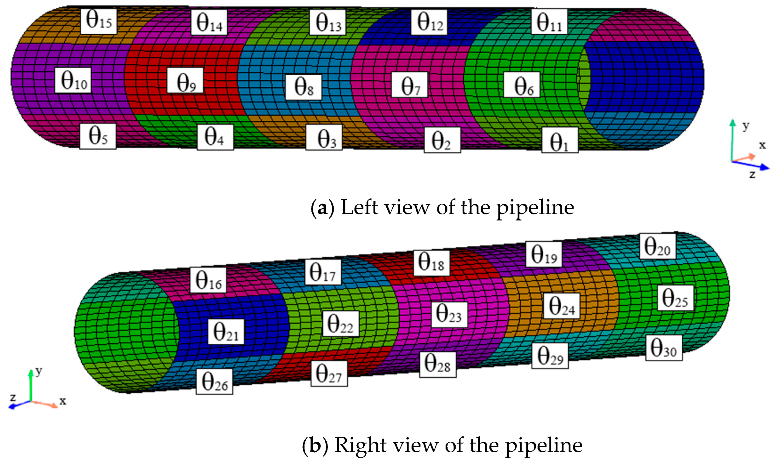
To simulate stiffness variations in the pipeline caused by manufacturing processes and factors such as corrosion during service, the pipeline is uniformly divided along its axial direction (z-axis) into 5 segments and hoop direction into 6 equal parts, resulting in a total of 30 regions. These regions are numbered sequentially as θ₁ to θ₃₀, as illustrated in Figure 3. The stiffness in each of these 30 regions is assumed to have changed, and the relative stiffness variation rates with respect to the initial values are treated as the parameters to be identified. The specific values are listed in

Table 1. Preset parameters.

No.	${\theta }_1$	${\theta }_2$	${\theta }_3$	${\theta }_4$	${\theta }_5$	${\theta }_6$	${\theta }_7$	${\theta }_8$	${\theta }_9$	${\theta }_{10}$
Parameter value	0.25	−0.2	−0.1	0.15	0.2	0.3	−0.2	−0.05	−0.05	0.2
	${\theta }_{11}$	${\theta }_{12}$	${\theta }_{13}$	${\theta }_{14}$	${\theta }_{15}$	${\theta }_{16}$	${\theta }_{17}$	${\theta }_{18}$	${\theta }_{19}$	${\theta }_{20}$
	−0.1	0.1	−0.1	0.05	0.1	0	0.25	−0.15	−0.25	−0.1
	${\theta }_{21}$	${\theta }_{22}$	${\theta }_{23}$	${\theta }_{24}$	${\theta }_{25}$	${\theta }_{26}$	${\theta }_{27}$	${\theta }_{28}$	${\theta }_{29}$	${\theta }_{30}$
	0.05	−0.25	−0.2	0.1	−0.25	−0.15	−0.15	−0.25	0.15	0.2

.

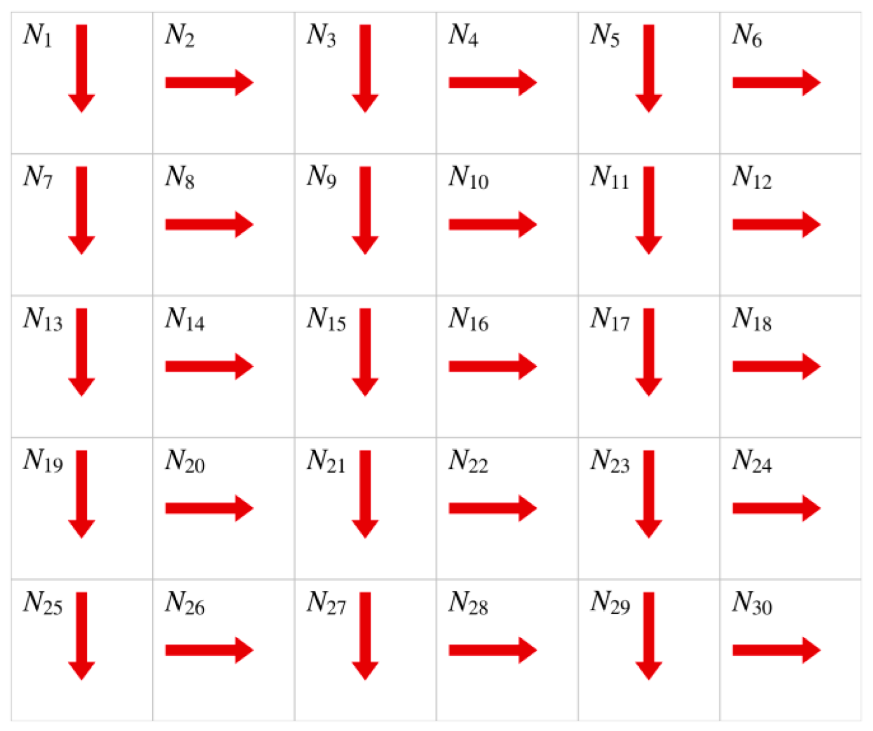
Using the stiffness values specified in Table 1, the average strain values for the 30 regions of the pipeline under the same internal pressure are calculated. From these, 15 regions depicted in Figure 4 are selected for static strain measurements in the hoop direction (perpendicular to the z-axis), while the other 15 regions are selected for axial static strain measurements (parallel to the z-axis). Here, N₁ denotes the label for region 1, and so on. Additionally, to simulate measurement uncertainty, 1% Gaussian white noise is added to these strain values.

The average strain values computed using the preset parameters from Table 1 are presented in

Table 2. Static strain of each measured point (${\mathrm{\mu }}_{\mathrm{\epsilon }}$).

Node Number	N1	N2	N3	N4	N5	N6	N7	N8	N9	N10
Initial strain	55.06	1.16	51.00	1.16	55.06	24.22	92.47	8.53	92.47	24.22
Damage strain	57.81	1.08	42.52	1.10	43.38	20.74	123.40	7.78	73.88	22.35
Node number	N11	N12	N13	N14	N15	N16	N17	N18	N19	N20
Initial strain	62.60	27.46	56.23	27.46	62.60	26.90	58.66	26.23	58.66	26.90
Damage strain	57.26	29.97	51.13	27.52	68.81	37.34	49.63	25.23	56.70	33.98
Node number	N21	N22	N23	N24	N25	N26	N27	N28	N29	N30
Initial strain	82.58	10.90	98.89	10.90	82.58	5.26	52.91	0.76	52.91	5.26
Damage strain	112.27	8.37	90.93	11.83	105.34	4.53	46.22	0.65	62.99	6.53

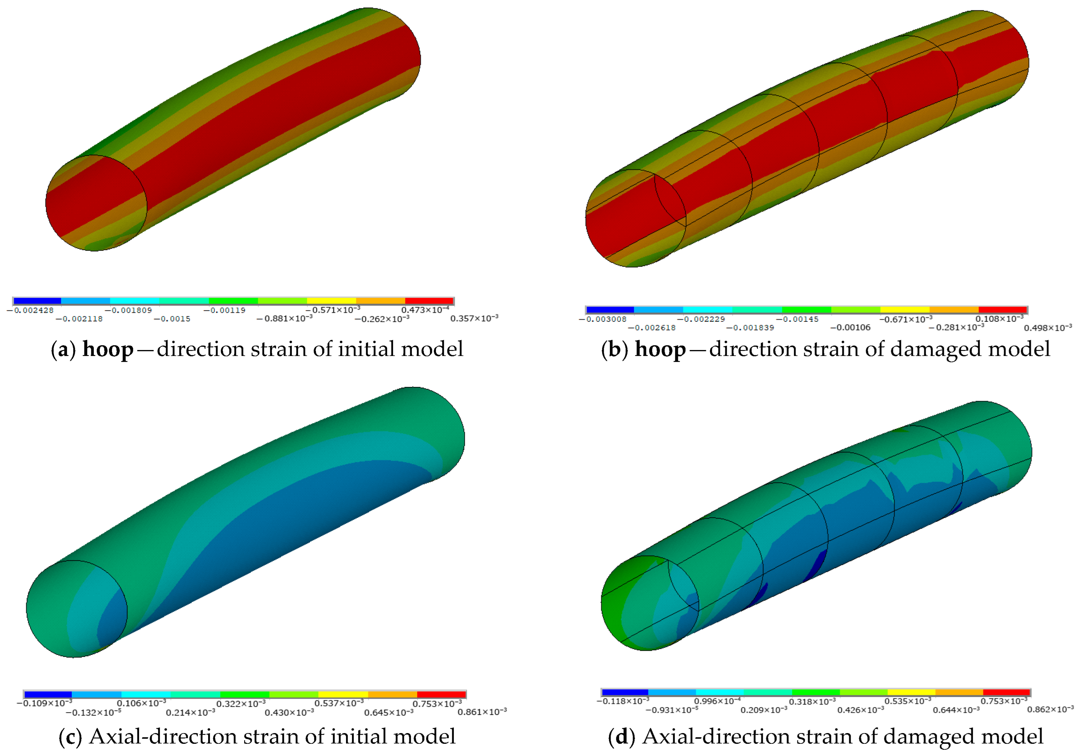
. As shown, the tensile strains in the hoop direction are particularly pronounced, whereas the axial strains are comparatively smaller. Figure 5 illustrates the strain distribution of the pipeline computed by ANSYS before and after the stiffness changes.

Considering the high dimensionality of the parameters to be identified, Latin Hypercube Sampling (LHS) was employed to generate 800 set of samples for training the DNN surrogate model. Corresponding static strain responses for these 800 sets of samples were computed using ANSYS. The first 700 sets of samples were used to fit the DNN surrogate model, while the remaining 100 sets of samples were used to validate its accuracy. No sequential or adaptive sampling techniques were employed during the data generation stage; all training samples were generated in a single LHS batch to ensure a uniform exploration of the prior parameter space.

The DNN surrogate model consisted of four hidden layers with 64, 128, 128, and 64 neurons, respectively. The ReLU activation function was used for all hidden layers, while a linear activation was applied to the output layer to predict continuous strain responses. The model was trained using the Adam optimizer with an initial learning rate of 1 × 10⁻³, a decay rate of 1 × 10⁻⁵, and a mini-batch size of 32. Early stopping was adopted with a patience of 50 epochs to prevent overfitting, and the final model parameters were selected based on the minimum validation loss.

Figure 6 presents the static strain predictions of the DNN surrogate model. The prediction accuracy was evaluated using mean squared error (MSE) and coefficient of determination (R²). As seen in Figure 6, the MSE values remain low across all subplots, while R² values approach 0.92. Only N₁₂ and N₁₇ exhibit a small but acceptable underestimation of strain, and no clustered or high-strain-region errors are observed, indicating that the DNN surrogate model provides highly accurate static strain predictions. This surrogate model will be employed in the subsequent MALA to compute pipeline strains.

After obtaining the accurate DNN surrogate model, the simulated strain measurement data under various operating conditions were input into Equation (5) to perform MALA sampling. Benefiting from AD, the Jacobian matrix can be obtained exactly and efficiently, which greatly enhances the stability and computational efficiency of the sampling process. For comparison, the DRAM sampling method was also employed to generate Markov chains for the parameters under the same conditions. During the MCMC sampling, all 30 parameters were assigned independent Gaussian prior distributions with zero mean and a standard deviation of 0.2, i.e., ${\theta }_i\sim \mathcal{N}\left(0,{0.2}^2\right)$. The step size in the Langevin proposal of the MALA was uniformly set to 1 × 10⁻⁴, which was calibrated through preliminary simulations. The test runs showed that step sizes within the range of 10⁻⁶ to 10⁻⁴ provided stable and efficient sampling, and the chosen value ensured rapid convergence without numerical instability. To further verify convergence, the posterior chains were evaluated using quantitative diagnostics such as the Gelman–Rubin statistic (R < 1.05 for all parameters) and effective sample size (ESS) estimates, both confirming that the sampling process had reached a stable posterior distribution. The Markov chains of all 30 parameters obtained from these two sampling methods are shown in Figure 7.

As seen in Figure 7a, the Markov chains generated by the DRAM method gradually converge to stable values after 20,000 iterations, but these values do not align well with the preset true values. This difference is particularly clear for parameters θ₄, θ₅, θ₁₅, θ₁₈, θ₁₉, θ₂₂, and θ₂₇–θ₃₀, where the long-run mean under DRAM remains clearly biased, whereas MALA tracks the preset values with much smaller fluctuations.

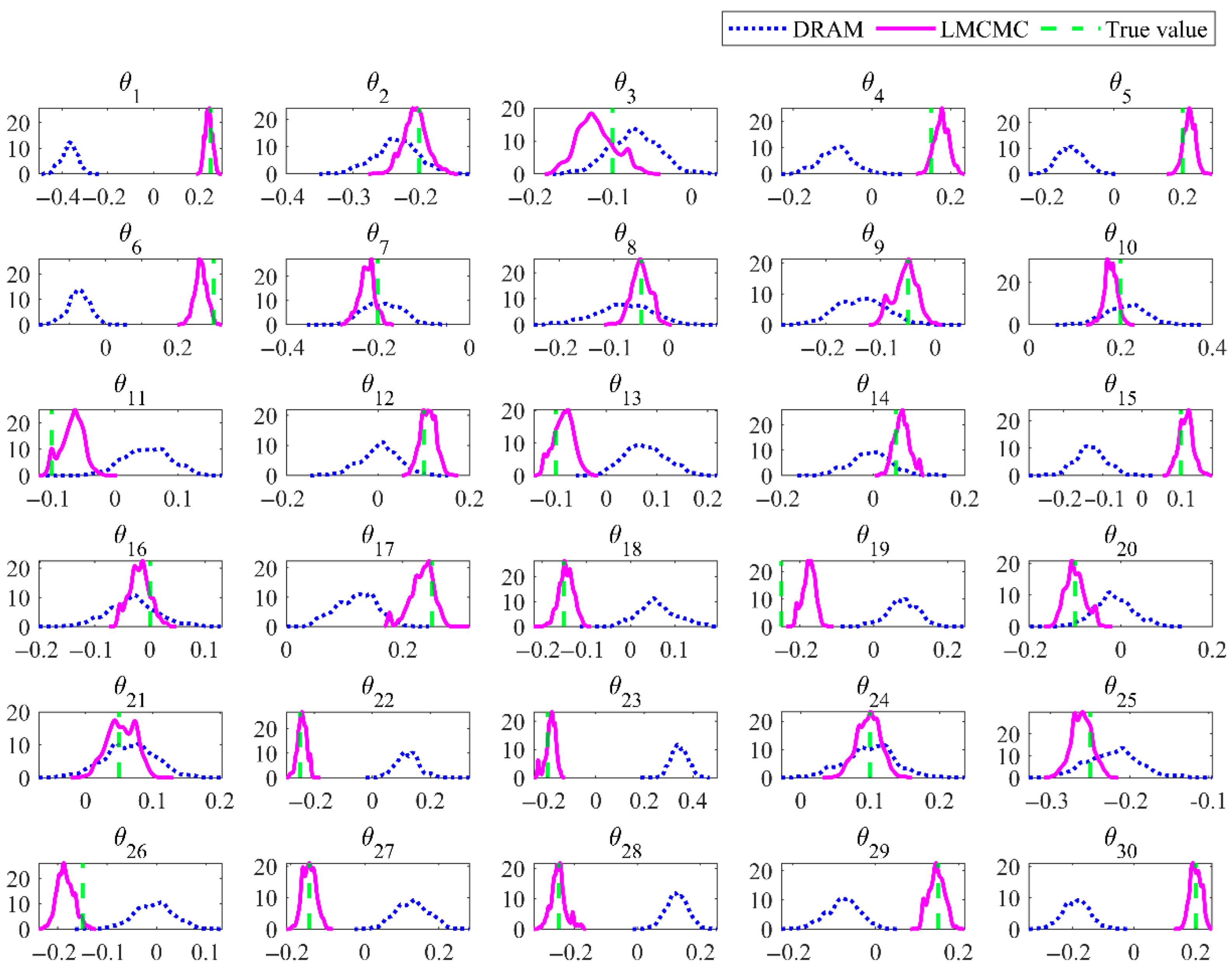
Figure 8 shows the PDFs of the identified parameters after discarding the first 20,000 samples as burn-in. Relative to the preset truths, DRAM yields broader and sometimes shifted distributions, while MALA produces sharply peaked and well-centered posteriors. The improvement is most obvious for θ₄, θ₅, θ₁₅, θ₁₈, θ₁₉, θ₂₂, and θ₂₇–θ₃₀, where DRAM’s posterior modes deviate noticeably and exhibit wide dispersion, whereas MALA’s posterior modes coincide closely with the true values, exhibiting much narrower credible intervals. Overall, these results clearly demonstrate that the proposed MALA-based inference achieves higher parameter accuracy and lower uncertainty compared with DRAM.

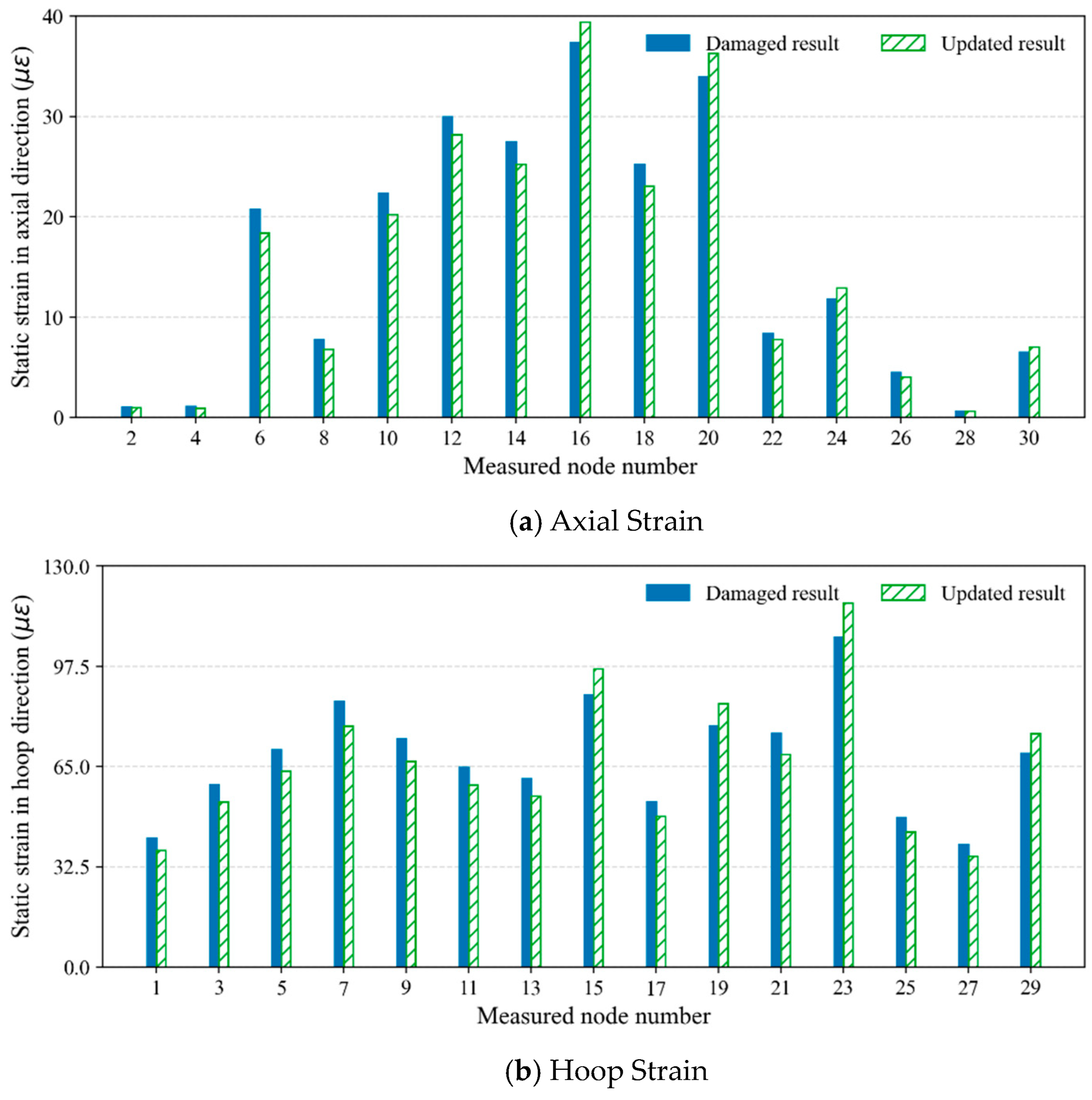
The identified parameters were substituted back into the FE model to compute the axial and hoop static strains of the pipeline, as shown in Figure 9. It can be observed that the strains calculated with the updated stiffness parameters closely match the simulated mean measured strains. This result further validates the effectiveness of the strain-based Bayesian model updating method for FE models of pipeline structures, especially under complex boundary conditions where other measurement indicators are not readily available. The updated model accurately reproduces the true structural strain states.

More importantly, in this case study, even with the high dimensionality of the parameters to be identified, the proposed Bayesian MALA method performs excellently. From the perspective of computational efficiency, all numerical experiments were conducted on a high-performance workstation equipped with an Intel Xeon E-2235 (Intel Corporation, Santa Clara, CA, USA) processor (6 cores, 12 threads), dual NVIDIA RTX 4000 GPUs (NVIDIA Corporation, Santa Clara, CA, USA), and 64 GB of RAM, providing robust computational capacity for large-scale model training and sampling tasks. Including the time for computing the training samples, the entire identification process was completed within 10 min. This outcome fully demonstrates the high computational efficiency of the proposed method, making it suitable for rapid parameter identification of large-scale industrial pipelines.

6.2. Influence of Measurement Strain Quantity and Direction on Identification Results

During strain testing of industrial pipelines, the number and orientation of gauges exert a pronounced influence on parameter identification. To clarify this effect, three measurement cases are studied. The configuration described in Section 6.1 is adopted as Case 1, in which strain gauges are uniformly deployed in both the axial and hoop directions across 15 circumferential regions. Two alternative cases are considered for comparison. In Case 2 only hoop strains from the same 15 regions are recorded, whereas Case 3 relies exclusively on axial strains. Apart from this difference in measurement layout, all modelling settings—including boundary conditions, material properties and a 1% Gaussian noise level—are identical among the three cases.

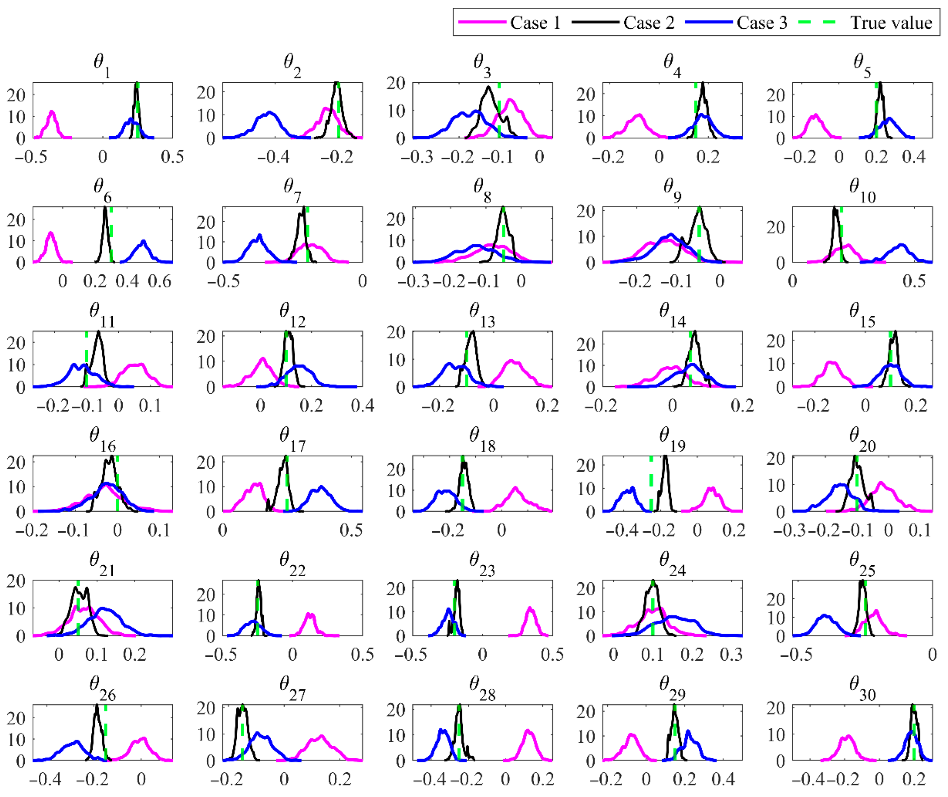
For each case, posterior parameter distributions are obtained from MCMC sampling. After discarding the first 50% of each chain as burn-in, the remaining samples are used to compute the posterior means and variances, which are summarised in Figure 10. Case 1 reproduces the prescribed parameter field most faithfully: the posterior means coincide with the true values in all but region 19, and the associated variances are the smallest of the three cases. This outcome highlights the value of rich, multidirectional data for tightening the inverse solution. When only circumferential strains are employed (Case 2), satisfactory accuracy is retained in most regions, yet noticeable biases arise in regions 1, 6, 8, 10, 12, 17, 19 and 25. Axial strains alone (Case 3) lead to an even higher frequency of misidentification, reflecting their lower sensitivity to stiffness variations.

The results demonstrate that hoop strains react more strongly to changes in structural parameters and therefore yield superior identification when available. Relying on a single strain component, by contrast, increases uncertainty and the risk of parameter misclassification. Consequently, in the subsequent experimental programme both axial and hoop strains are collected to ensure accurate and reliable identification of the pipeline’s mechanical parameters.

7. Experimental Case Study

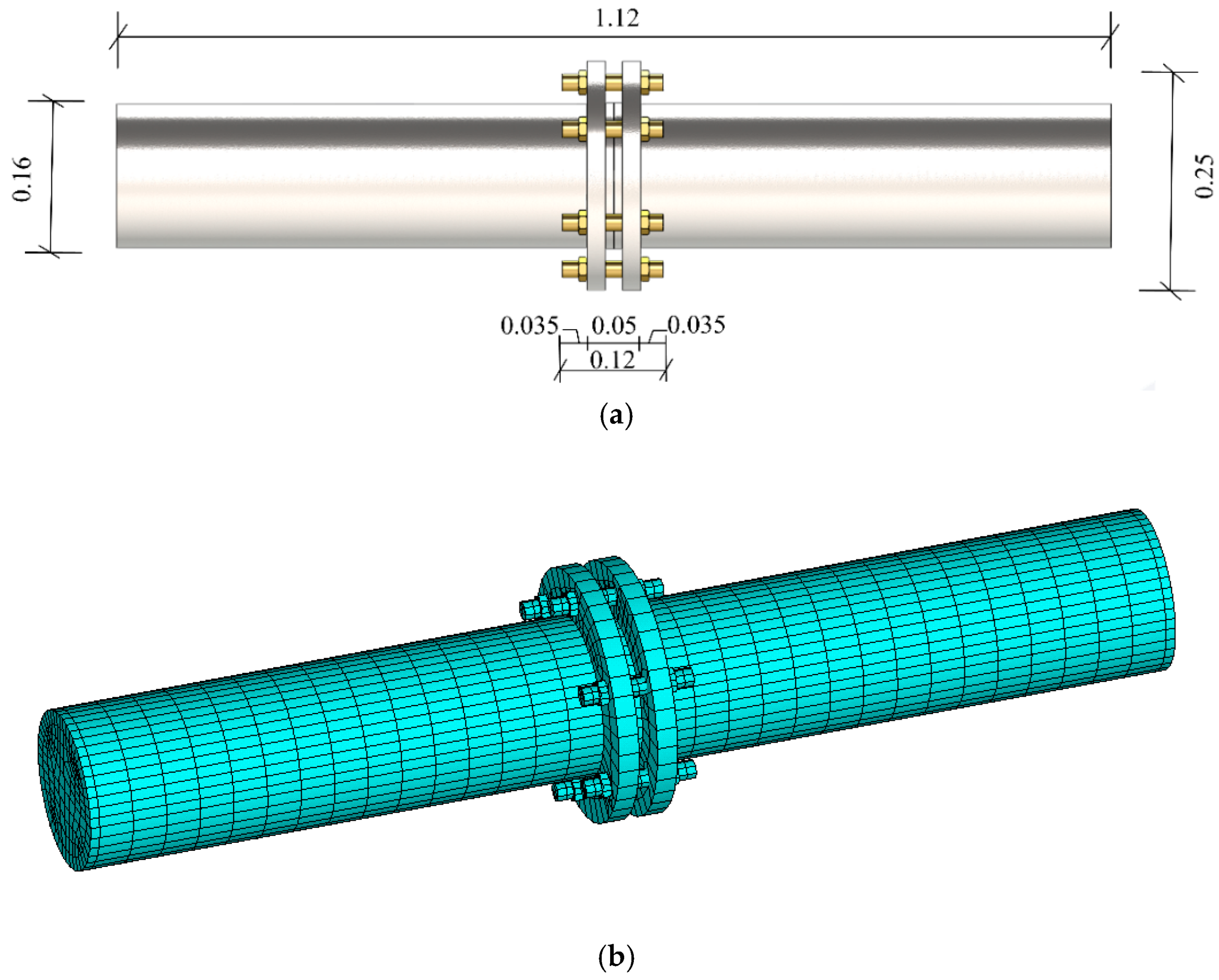
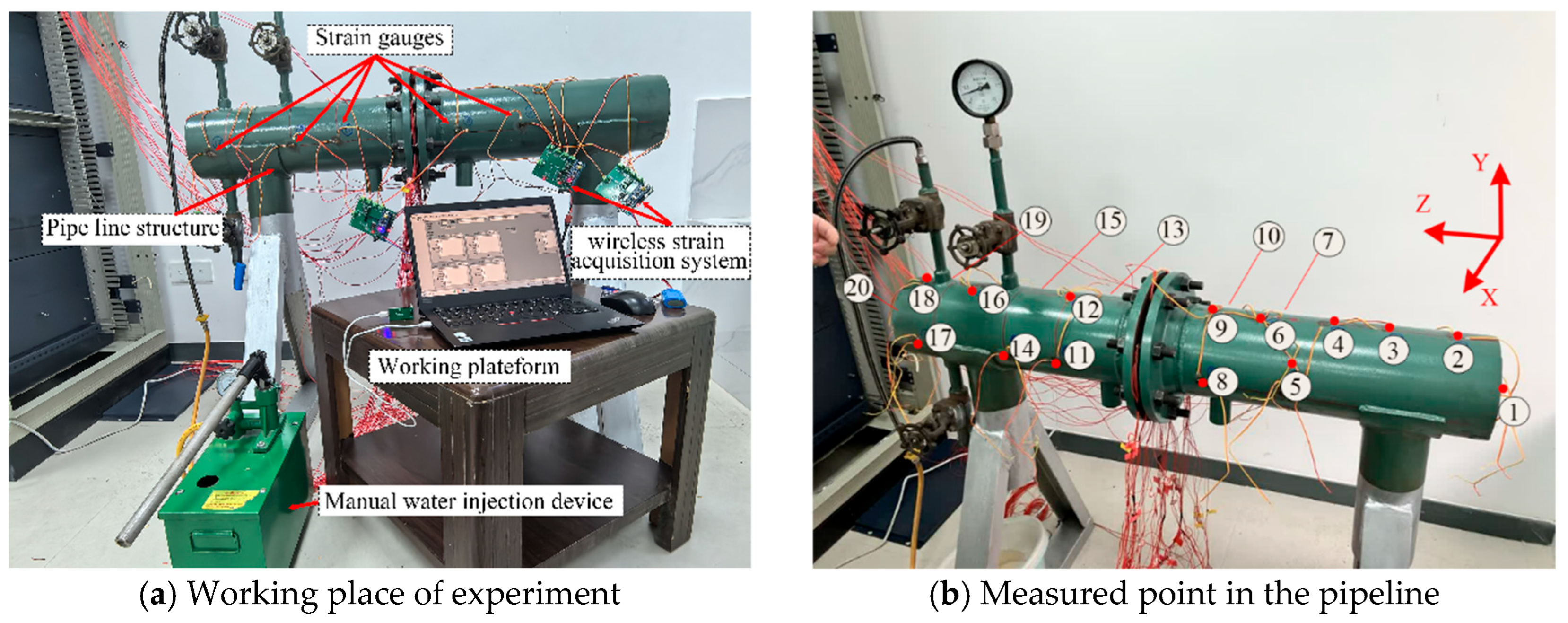
A real pipeline structure was constructed to validate the proposed method. The pipeline system comprises two segments of seamless carbon steel pipes, each with an outer diameter of 160 mm and a wall thickness of 15 mm, as depicted in Figure 11a. These pipe segments are interconnected using flat flanges, which are constructed from Q235 carbon steel, with an outer diameter of 250 mm and a thickness of 17 mm. Each flange features six evenly spaced bolt holes, each with a diameter of 20 mm.

Based on the above dimensions of the pipeline, a FE model of the pipeline system was developed using ANSYS software, as illustrated in Figure 11b. The pipeline, flanges, and bolts were modeled using SOLID186 solid elements, with each element having 20 nodes, to ensure accurate calculations of stress distribution. The material properties of the pipeline include a Young’s modulus of 2.06 × 10¹¹ Pa, a Poisson’s ratio of 0.3, and a density of 7850 kg/m³. The contact interactions between the bolts and flanges were simulated using CONTA174 and TARGE170 elements. The pipeline is supported by brackets on both sides. The FE model consists of a total of 9893 elements and 21,274 nodes.

The flanges were modeled with refined meshes near bolt holes to capture local stress concentrations, and each bolt was preloaded with an axial tensile force of 12 kN to reproduce the tightening condition. The contact behavior between bolt heads, nuts, and flange surfaces was set to frictional, with a coefficient of friction of 0.15. The supporting brackets were modeled as steel plates with fixed constraints at their base and surface contact coupling with the outer pipeline wall, allowing vertical displacement while constraining rotation. The fluid inside the pipe was represented by an equivalent internal pressure load of 0.3 MPa applied on the inner wall. The load–displacement convergence criterion was set to 10⁻³ for nonlinear solution stability.

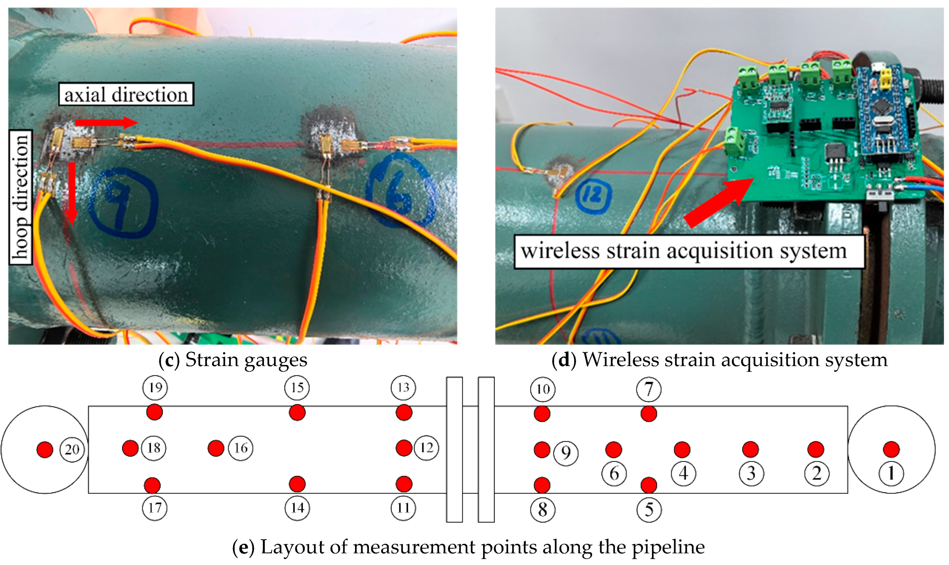
The experimental setup is shown in Figure 12a. To comprehensively capture strain data from various regions of the pipeline, the experiment employed a uniform measurement point distribution strategy, selecting 20 locations for strain gauge placement, as illustrated in Figure 12b–e. At each location, two strain gauges were installed to measure strains in the axial and hoop directions, respectively. A custom-developed wireless strain acquisition system was used to collect and store strain data from all 40 measurement channels. The coordinates of these measurement points are listed in

Table 3. Measurement Point Coordinates (m).

Node	x	y	z	Node	x	y	z
1	0	0	0	11	0.085	0	0.70
2	0	0.085	0.05	12	0	0.085	0.70
3	0	0.085	0.15	13	−0.085	0	0.70
4	0	0.085	0.27	14	0.085	0	0.81
5	0.085	0	0.34	15	−0.085	0	0.81
6	0	0.085	0.38	16	0	0.085	1.02
7	−0.085	0	0.38	17	0.085	0	1.07
8	0.085	0	0.49	18	0	0.085	1.07
9	0	0.085	0.49	19	−0.085	0	1.07
10	−0.085	0	0.49	20	0	0	1.12

.

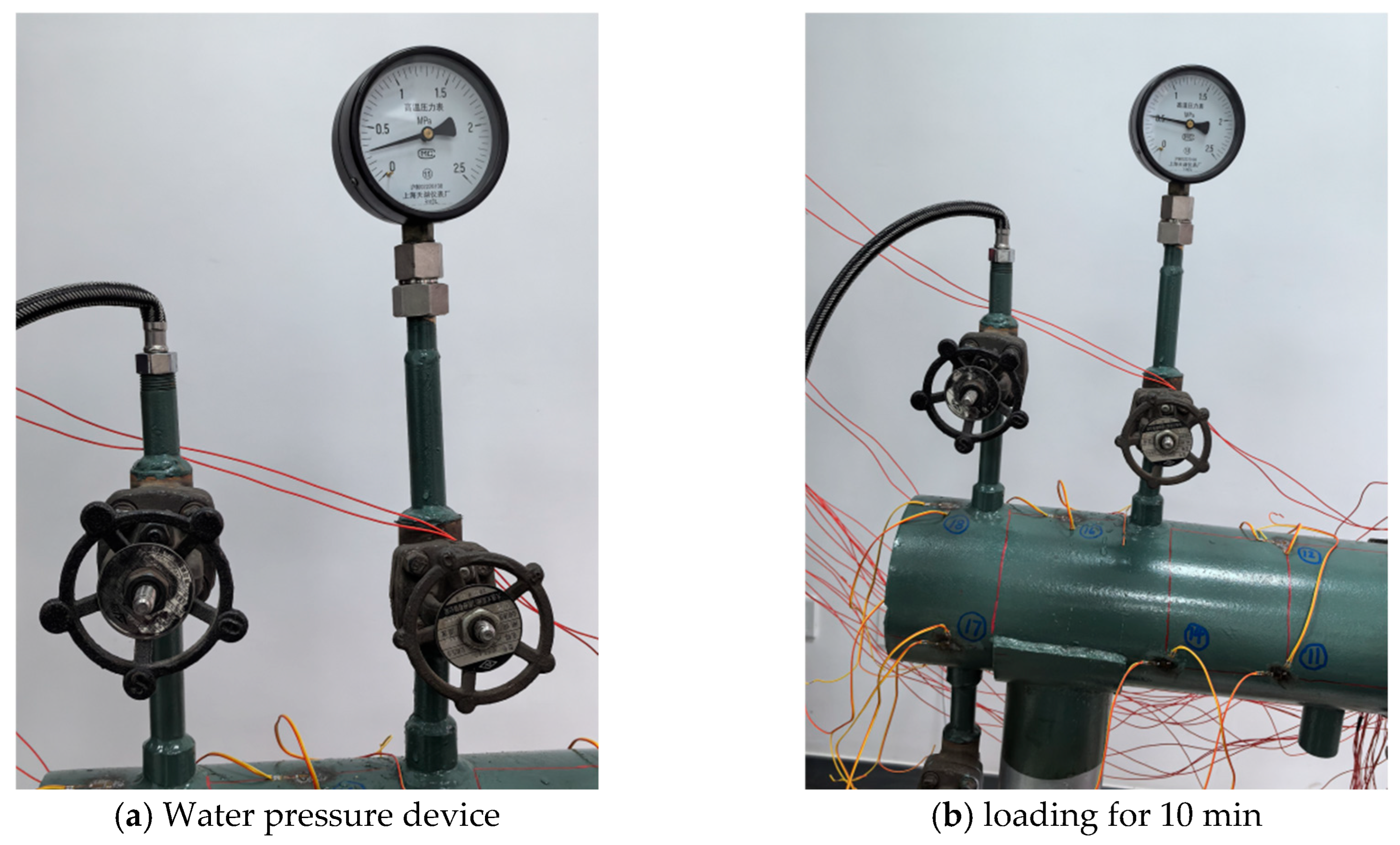
Before the experiment commenced, the pipeline was filled with water, the pressure gauge was calibrated to zero, and the wireless strain acquisition system was initialized to record zero strain values. Subsequently, static hydrostatic loading was applied to the pipeline. Water pressure was incrementally increased manually using the device depicted in Figure 13a, with pressure increments controlled to occur approximately once per second. Each pressure increment resulted in an increase in the gauge reading of about 0.1 MPa. The wireless strain acquisition system automatically recorded strain variations across all 40 channels throughout the loading process. During the experiment, careful monitoring of the pipeline’s deformation was conducted, and inspections were performed to ensure there were no leaks. The loading continued until the pressure reached 0.5 MPa, which was then sustained for a period of 10 min, as illustrated in Figure 13b.

Table 4. Static strain of each measured point (${\mathrm{\mu }}_{\mathrm{\epsilon }}$).

Node No.	1-x	2-x	3-x	4-x	5-x	6-x	7-x	8-x	9-x	10-x
FEM	4.35	3.18	5.19	7.95	7.56	10.4	4.12	8.11	11.50	4.50
Measured	4.27	3.14	5.39	7.90	9.40	12.9	5.05	9.66	13.40	5.22
Node No.	11-x	12-x	13-x	14-x	15-x	16-x	17-x	18-x	19-x	20-x
FEM	7.60	13.2	5.09	7.37	4.62	6.92	1.47	4.23	1.76	5.95
Measured	9.12	15.5	5.89	9.29	5.66	7.64	1.54	4.41	1.98	5.59
Node No.	1-y	2-y	3-y	4-y	5-y	6-y	7-y	8-y	9-y	10-y
FEM	1.69	1.18	1.97	3.04	3.59	4.20	1.40	3.72	5.01	1.67
Measured	2.81	1.70	2.50	3.13	4.61	5.25	1.83	4.52	5.75	2.05
Node No.	11-y	12-y	13-y	14-y	15-y	16-y	17-y	18-y	19-y	20-y
FEM	3.81	5.48	1.88	3.49	1.61	2.64	1.42	1.49	1.08	2.04
Measured	4.41	6.41	2.28	4.51	2.03	3.07	2.22	2.00	1.20	3.01

presents the strain values measured at pressure gauge readings of 0.25 MPa and 0.5 MPa, alongside the computed strain values from the initial FE model under the same pressures. As shown in Table 4, the overall strain trends between the initial FE model and measurements are generally consistent. Measurement points 9 and 12 exhibit relatively large axial and hoop strains, with longitudinal strains approximately twice those of the tangential strains. However, compared to measured results, the simulation generally shows an increasing trend in strain at most measurement points, indicating that the initial FE model does not accurately capture the true strain response of the pipeline. Therefore, it is necessary to identify the actual stiffness of the experimental pipeline structure using the proposed method.

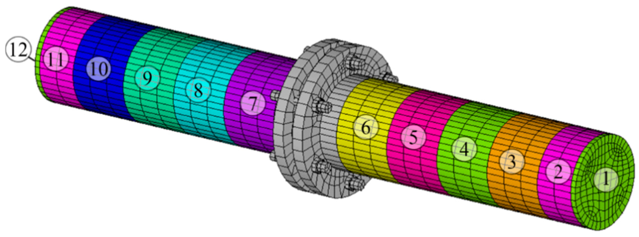
Considering the discrete spatial distribution of measurement points and local variations in pipeline geometry, the experimental pipeline is divided into 12 regions according to measurement locations (see Figure 14). During long-term service, factors such as wall thickness reduction, outer diameter deviation, and fluctuations in material elastic modulus alter the overall mechanical response of the pipeline. These changes can ultimately be represented as equivalent stiffness variations at the structural level. To avoid the complexity of identifying numerous uncertain variables such as thickness, diameter, and material properties separately, an equivalent stiffness modeling strategy is adopted here: each region is treated as an equivalent segment with uniform mechanical properties, characterized by a single parameter θ_i (i = 1, 2, …, 12) that comprehensively reflects the combined effects of geometry and material in that region. Thus, 12 parameters {θ₁, θ₂, …, θ₁₂} are to be identified.

By substituting the 40 measured strain values from 20 measurement points listed in Table 4 and their corresponding computed strain values into Equation (2) to construct the likelihood function, Bayesian sampling was performed using the MALA with 100,000 iterations, where each of the 12 parameters was assigned an independent Gaussian prior with zero mean and a standard deviation of 0.2 (θ_i ∼ $𝒩$(0, 0.2²)). The DNN surrogate model employed for this experimental case used a slightly lighter architecture of three hidden layers with 64, 64, and 32 neurons, respectively, also adopting the ReLU activation function and a linear output layer. 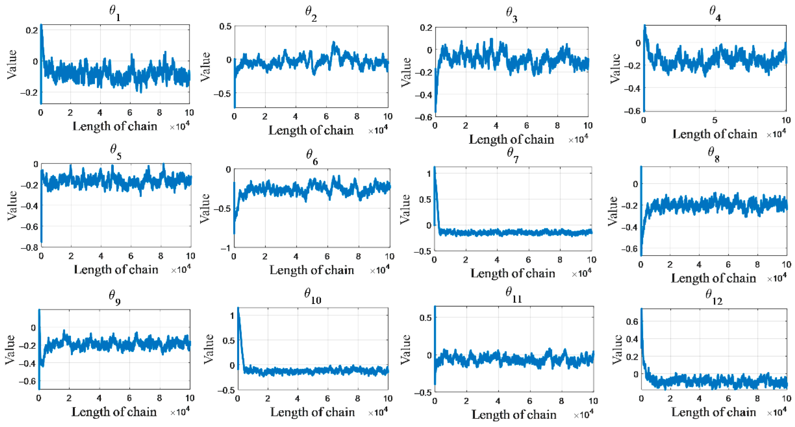The model was trained using the Adam optimizer with a learning rate of 1 × 10⁻³ and a batch size of 16. Early stopping with a patience of 30 epochs was applied to maintain generalization. 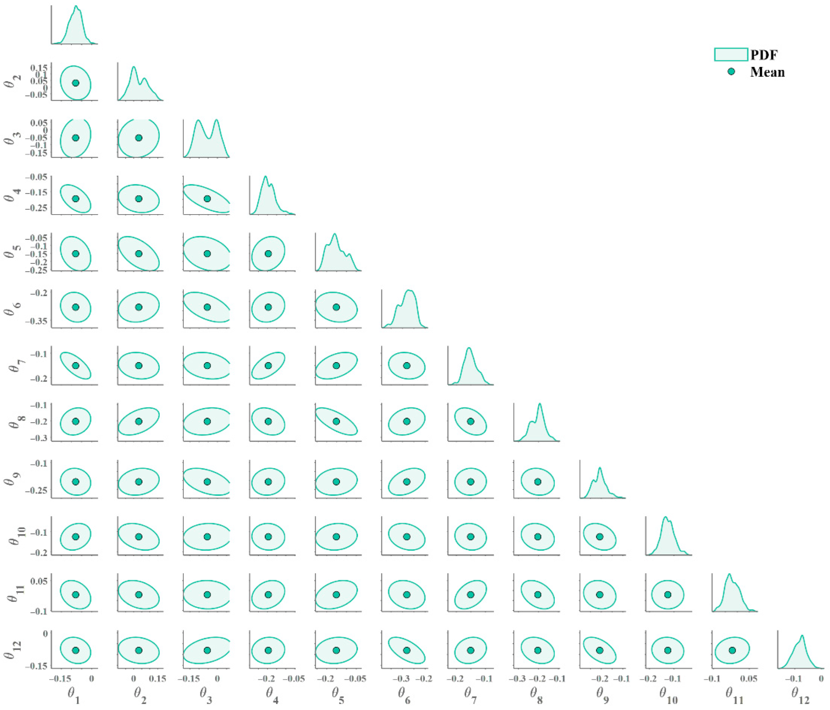The resulting Markov chains of the 12-dimensional equivalent stiffness parameter vector are shown in Figure 15. It can be observed that most chains enter a steady state after approximately 20,000 iterations, indicating that the posterior distribution has essentially converged. After discarding the first 20,000 samples as burn-in, the mean of the remaining samples is computed, with results presented in Figure 16.

As shown in Figure 16, most pipeline segments exhibit a reduction in equivalent stiffness, with decreases ranging from approximately −0.3 to −0.1. This finding indicates that the Bayesian sampling-based updating to the equivalent stiffness parameters better reflect the actual physical conditions of the pipeline design and operation, likely due to improved modeling of the underlying physical processes. Notably, regions 5, 6, 7, and 8 show the largest reductions, suggesting significant stiffness variations in these areas.

Additionally, the posterior PDFs for regions 2, 3, 5, 6, and 8 exhibit multimodal behavior, particularly pronounced in regions 2 and 3. This multimodality indicates uncertainty in the stiffness parameter estimates for these regions, potentially arising from more complex physical phenomena or heterogeneous material characteristics.

The multimodal patterns observed in regions 2, 3, 5, 6, and 8 indicate that multiple parameter combinations can reproduce the measured responses with comparable accuracy, implying partial non-uniqueness and correlation among parameters. Although MALA is a gradient-based sampler, its stochastic Metropolis–Hastings acceptance allows it to escape local modes, while the smooth DNN surrogate provides accurate gradient information that guides efficient movement across neighboring modes. Consequently, the DNN-based gradient guidance acts as a physical interpreter, helping the sampler traverse low-probability barriers and achieve balanced exploration of the multimodal posterior space.

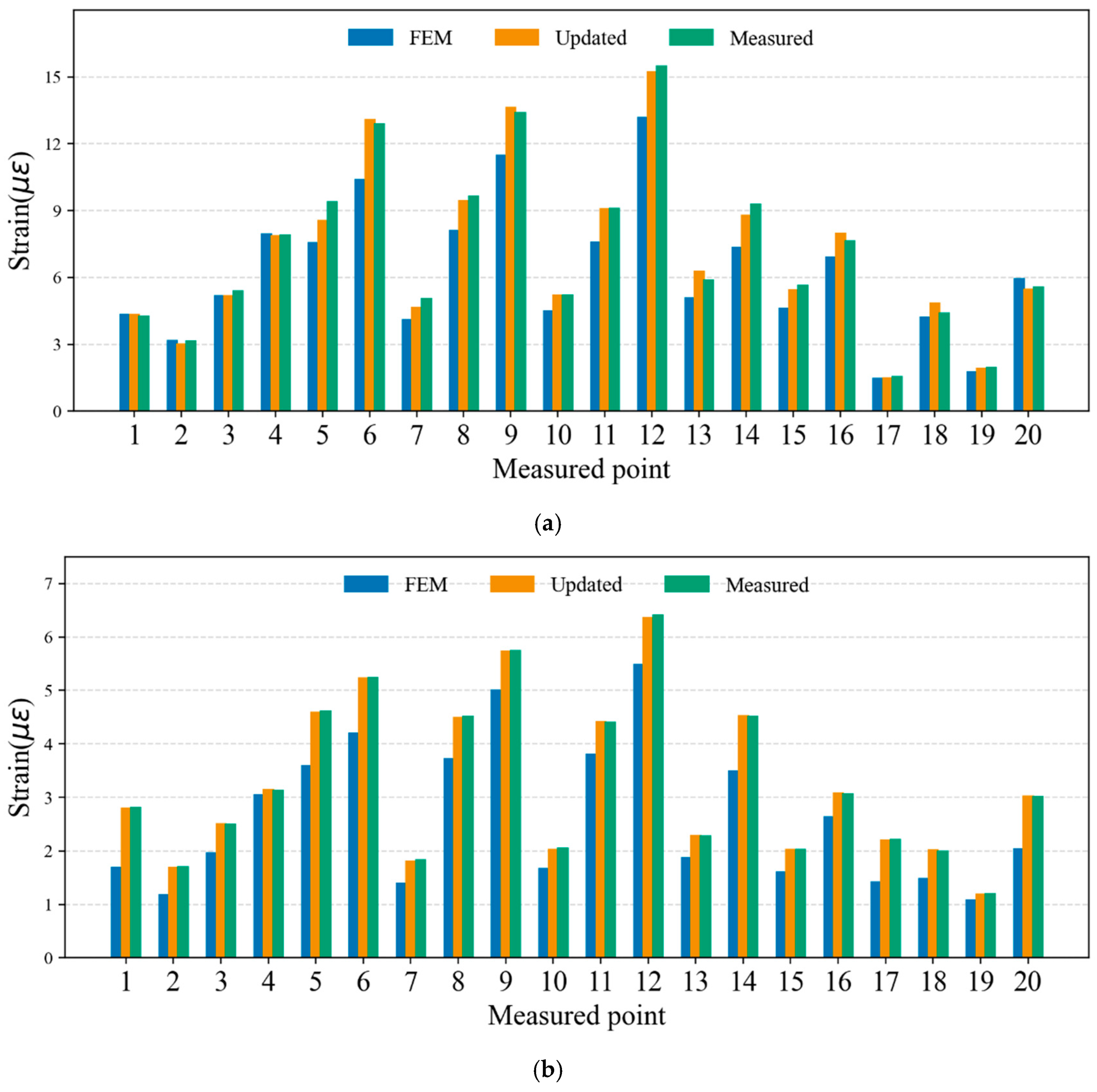
To validate the effectiveness of the identified parameters, the mean values of the equivalent stiffness parameters were substituted back into the FE model to recalculate the pipeline’s strain response under the same loading conditions. These recalculated strains were compared with the measured data collected by the wireless strain sensors, as shown in Figure 17.

From Figure 17a, which compares axial strains, it is evident that the original FE model shows significant deviations from the measurements at several points, especially in strain concentration areas (measurement points 6–12), where discrepancies are particularly pronounced. In contrast, the updated model, using the identified parameters, closely matches the measured strains, with the maximum relative error reduced from over 30% to less than 5%. Figure 17b shows similar trends for the hoop strains: the updated model accurately captures the actual strain distribution at all 20 measurement points, with notably improved prediction accuracy in peak regions (points 6, 8, 10, and 12).

These results demonstrate that the equivalent stiffness parameters obtained through Bayesian inversion not only quantify the equivalent stiffness of each segment but also enable the FE model to accurately reproduce the true mechanical response of the pipeline. This provides a reliable numerical foundation for subsequent structural safety assessments and residual life predictions.

Nevertheless, it should be noted that certain uncertainties remain. The identified parameters are affected by the accuracy of strain measurements, the assumed boundary conditions, and possible simplifications in the FE model. In addition, the DNN surrogate introduces minor approximation errors, which may slightly influence the posterior estimation. These factors may lead to localized deviations, especially under complex stress states or unmodelled external constraints, and will be addressed in future studies through improved sensor calibration and model refinement.

8. Conclusions

To address the challenges of structural parameter identification under complex boundary conditions, this study proposes an innovative Bayesian model updating method based on static strain data. This approach offers a promising solution in scenarios where traditional FE model updating methods struggle to effectively utilize static displacement or modal measurements. To efficiently handle high-dimensional parameter identification problems, the study employs Langevin MCMC sampling and innovatively integrates a deep neural network surrogate model, significantly accelerating the MCMC process.

The effectiveness of the proposed method is validated through numerical examples on pipeline structures. The results demonstrate that the constructed DNN surrogate model, mapping 30 equivalent stiffness parameters corresponding to pipeline regions to static strains, together with the MALA sampling method, exhibits outstanding performance in high-dimensional parameter spaces. The approach achieves superior convergence stability and identification accuracy, successfully recovering the equivalent stiffness parameters of the 30 regions with high agreement to the preset values. Moreover, the findings reveal that simultaneously utilizing strain data from both axial and tangential directions yields the best identification results, providing critical guidance for sensor placement in practical engineering applications.

The experimental case study using an actual pipeline structure further validates the effectiveness of the proposed method. The experimental results demonstrate that, for complex pipeline structures, the method can effectively handle multi-parameter identification problems, achieving refined FE model updating of the pipeline. The updated model accurately predicts measured strains, with the average absolute error significantly reduced from 27.3% to 4.2%.

Although the overall identification accuracy is high, several limitations should be acknowledged. The method assumes that the boundary conditions and material properties are precisely known, which may not always hold in practical applications. Furthermore, the surrogate model’s generalization depends on the representativeness of the training data, and the fixed step size in MALA may not be optimal for all configurations. These uncertainties could slightly affect the convergence speed and local estimation accuracy, but they do not compromise the overall conclusions of this study. Future work will focus on adaptive step-size control and probabilistic model validation to further improve robustness.

The main innovations and contributions of this study are as follows:

(1)

For the first time, the Metropolis-Adjusted Langevin Algorithm (MALA) is combined with a deep neural network (DNN) surrogate model, effectively overcoming the curse of dimensionality inherent in high-dimensional parameter identification.

(2)

A Bayesian inference framework based on static strain data is established, providing a novel technical approach to address structural parameter identification problems under complex boundary condition constraints.

(3)

The feasibility and accuracy of the proposed method are systematically validated through numerical examples and experimental cases, offering a solid and reliable basis for structural safety assessment in engineering applications.

In summary, when static displacement or modal testing is limited by complex boundary conditions, the static strain-based FE model updating method proposed herein represents a highly competitive alternative. Future research will focus on extending this method to a wider range of practical engineering structures, such as large-scale pipeline systems and pressure vessels, aiming to provide dependable technical support for the safety evaluation of these critical infrastructures and contribute to advancements in the field of structural health monitoring.