Article

Physics-Informed Multi-Task Neural Network (PINN) Learning for Ultra-High-Performance Concrete (UHPC) Strength Prediction

1
School of Architecture Engineering, Shaanxi A&F Technology University, Xianyang 712100, China
2
Shaanxi Construction Engineering Group No. 5 Construction Co., Ltd., Xi’an 710032, China
*
Author to whom correspondence should be addressed.
Buildings 2025, 15(23), 4243; https://doi.org/10.3390/buildings15234243
Submission received: 24 September 2025 / Revised: 20 November 2025 / Accepted: 22 November 2025 / Published: 24 November 2025
(This article belongs to the Special Issue Trends and Prospects in Cementitious Material)

Abstract

Ultra-high-performance concrete (UHPC) mixtures exhibit tightly coupled ingredient–property relations and heterogeneous reporting, which complicate the data-driven prediction of compressive and flexural strength. We present an end-to-end framework that (i) harmonizes mixture records, (ii) completes numeric features using a dependence-preserving Gaussian copula routine, and (iii) standardizes/encodes predictors with training-only fits. The feature space focuses on domain ratios and concise interactions (water–binder, superplasticizer–binder, total fiber, water–binder, superplasticizer–binder, and fiber normalized by water–binder). A physics-informed multi-task neural network (PINN) is trained in log space with Smooth-L1 supervision and learned per-task noise scales for uncertainty-weighted balancing, while soft monotonicity penalties are applied to input gradients so that predicted strength is non-increasing in water–binder (both targets) and, when available, non-decreasing in fiber content for flexural response. In parallel, histogram-based gradient boosting is fitted per target; a convex combination is then selected on the validation slice and fixed for testing. On the held-out sets, the blended model attains an MAE/RMSE/R2 of 10.86 MPa/14.68 MPa/0.848 MPa for compressive strength and 2.78 MPa/3.67 MPa/0.841 MPa for flexural peak, improving over the best single family by 0.5 RMSE (compressive) and 0.16 RMSE (flexural), with corresponding R2 gains of 0.01–0.02. Residual-versus-prediction diagnostics and predicted–actual overlays indicate aligned trends and reduced heteroscedastic tail errors.

1. Introduction

Ultra-high-performance concrete (UHPC) combines an exceptionally low water-to-binder ratio, dense particle packing, and discrete fibers to deliver superior compressive and flexural properties together with long-term durability [1,2]. These attributes enable slender members, longer spans, and extended service life in both new construction and rehabilitation [3]. In prevailing practice, UHPC is often defined operationally as mixtures reaching ≥120 MPa 28-day compressive strength under standard curing, with numerous deployments in bridges and rehabilitation projects [4,5,6]. Realizing these benefits, however, requires navigating a high-dimensional, tightly coupled design space in which small changes in proportions or curing can propagate nonlinearly to fresh behavior and hardened responses [7,8,9].
Progress in mix design is slowed by two practical bottlenecks. Firstly, standardized tests impose long feedback cycles—for example, compressive and flexural tests at 28 days (ASTM C109/C1609 [10,11]) and sulfate attack protocols that can last months (ASTM C1012 [12])—which delay hypothesis evaluation [13]. Secondly, as binders, fillers, admixtures, and fiber parameters multiply, experimental design becomes combinatorial; multi-source datasets are heterogeneous, include missing entries, and exhibit unit or naming inconsistencies. Aggregating results across laboratories further introduces inter-laboratory variability and heterogeneous metadata, complicating harmonization and amplifying overfitting risks [14].
A complementary route is to learn predictive mappings that jointly estimate compressive and flexural responses from mixture and processing descriptors [15,16]. Because the two targets share physical determinants yet differ in sensitivity (e.g., fiber effects are typically stronger in flexure), multi-task learning is attractive [17]. Crucially, learned response surfaces should respect first-order domain knowledge—non-increasing strength with increasing water-to-binder ratio and non-decreasing flexural capacity with increasing fiber content—to remain trustworthy within the observed design envelope [18]. These monotonic expectations are intended as first-order priors within the practically observed envelope, not as global laws beyond it [19].
Prior studies span linear or elastic net regressions, tree ensembles, and deep networks; multi-task formulations and physics-informed learning have also been explored [20,21]. However, three systemic gaps persist in UHPC pipelines: (i) dependence-blind imputation that distorts cross-feature relationships [22]; (ii) hand-tuned task weights that destabilize multi-task training under heteroscedastic noise [23]; and (iii) omitted monotonic priors, which can yield counter-physical gradients in data-sparse regions and limit auditability [24].
We therefore seek a predictor that is accurate and physics-consistent under heterogeneous, partially missing data. Specifically, we address the following: (1) copula-based, dependence-preserving imputation for numeric features; (2) uncertainty-weighted multi-task training to handle heteroscedastic noise; (3) monotonic gradient penalties to curb counter-physical behavior; and (4) comprehensive diagnostics—beyond a single headline metric—to audit model behavior [25,26].
Our end-to-end pipeline begins with Gaussian copula imputation to preserve cross-feature dependence [27]. Targets are modeled in log space via l o g ( 1 + y ) to mitigate heteroscedasticity and stabilize residuals across the strength range. A multi-task neural predictor is then trained with an uncertainty-weighted Huber objective—providing robustness to outliers and data-driven balancing [23]—while enforcing soft monotonicity (with respect to water-to-binder ratio and fiber content) through differentiable gradient penalties [24]. The architecture uses a Softplus head to ensure non-negative outputs and GELU + BatchNorm hidden layers to improve optimization stability without sacrificing flexibility. To complement smooth, physics-guided trends with sharp local interactions, we fit per-target histogram-based gradient boosting models and form a validation-selected convex blend with the neural predictions [28]. Training employs AdamW with gradient clipping, a Reduce-on-Plateau scheduler, early stopping, and seed ensembling; code, checkpoints, and figures are produced for full reproducibility [29,30].

2. Dataset

2.1. Source and Coverage

Data were obtained from a publicly curated, mixture-level repository of ultra-high-performance concrete (UHPC) mix designs (access and versioning details are provided in Data Availability). The corpus aggregates 2188 mix designs compiled from 168 publications across 27 countries and is organized under a harmonized schema of field names and units (kg/m3, %, mm, MPa) spanning five domains: mix constituents, curing, rheology, mechanical properties, and durability. For the present analysis, a deterministic ingestion workflow harmonized headers and data types to the repository specification without modifying any numerical values or units; each row represents a single UHPC mixture [31].
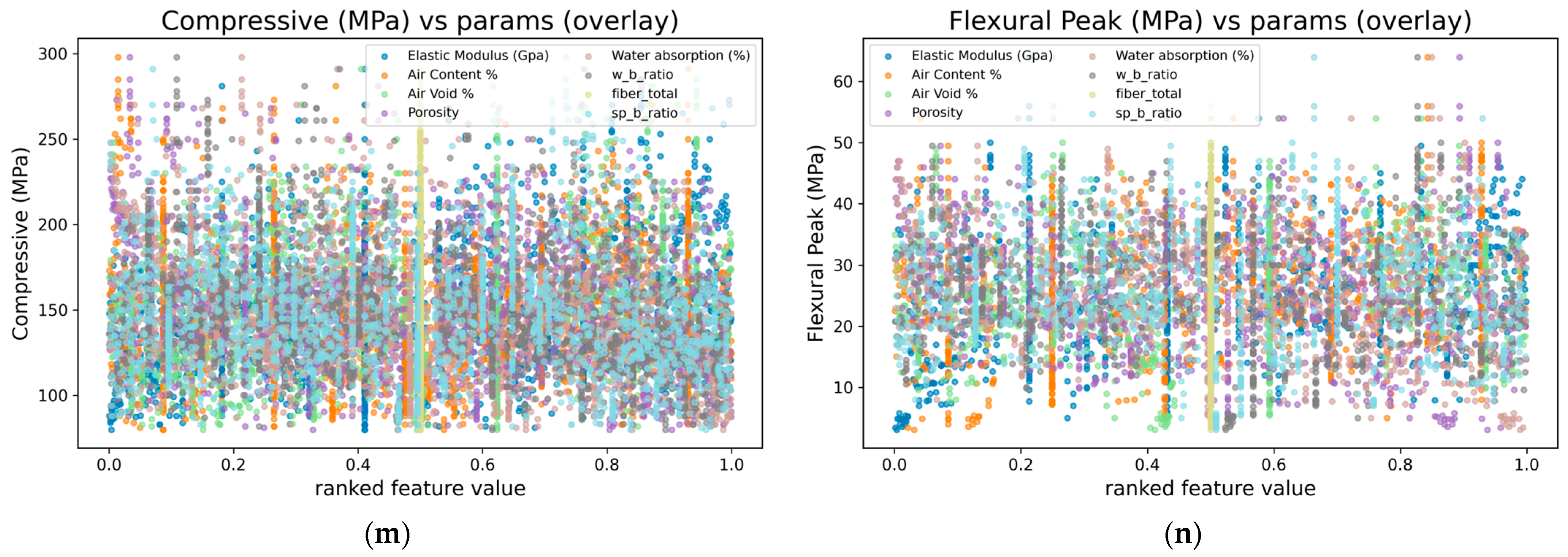
Figure 1 summarizes the empirical structure of the raw dataset using decile-binned scatterplots and rank overlay views. The univariate plots in Figure 1a–l relate compressive and flexural strengths to six covariates—water-to-binder ratio (w/b), porosity, water absorption, air content, air voids, and elastic modulus—and show broad coverage with long yet traceable tails. Directional tendencies are consistent with cementitious mechanics: strength generally decreases as w/b, porosity, or water absorption increase, and increases with elastic modulus (and, where available, higher fiber volume (%)); air-related indices exhibit predominantly negative associations. The rank overlays in Figure 1m,n confirm that these tendencies persist across quantiles rather than being driven by isolated outliers [32].
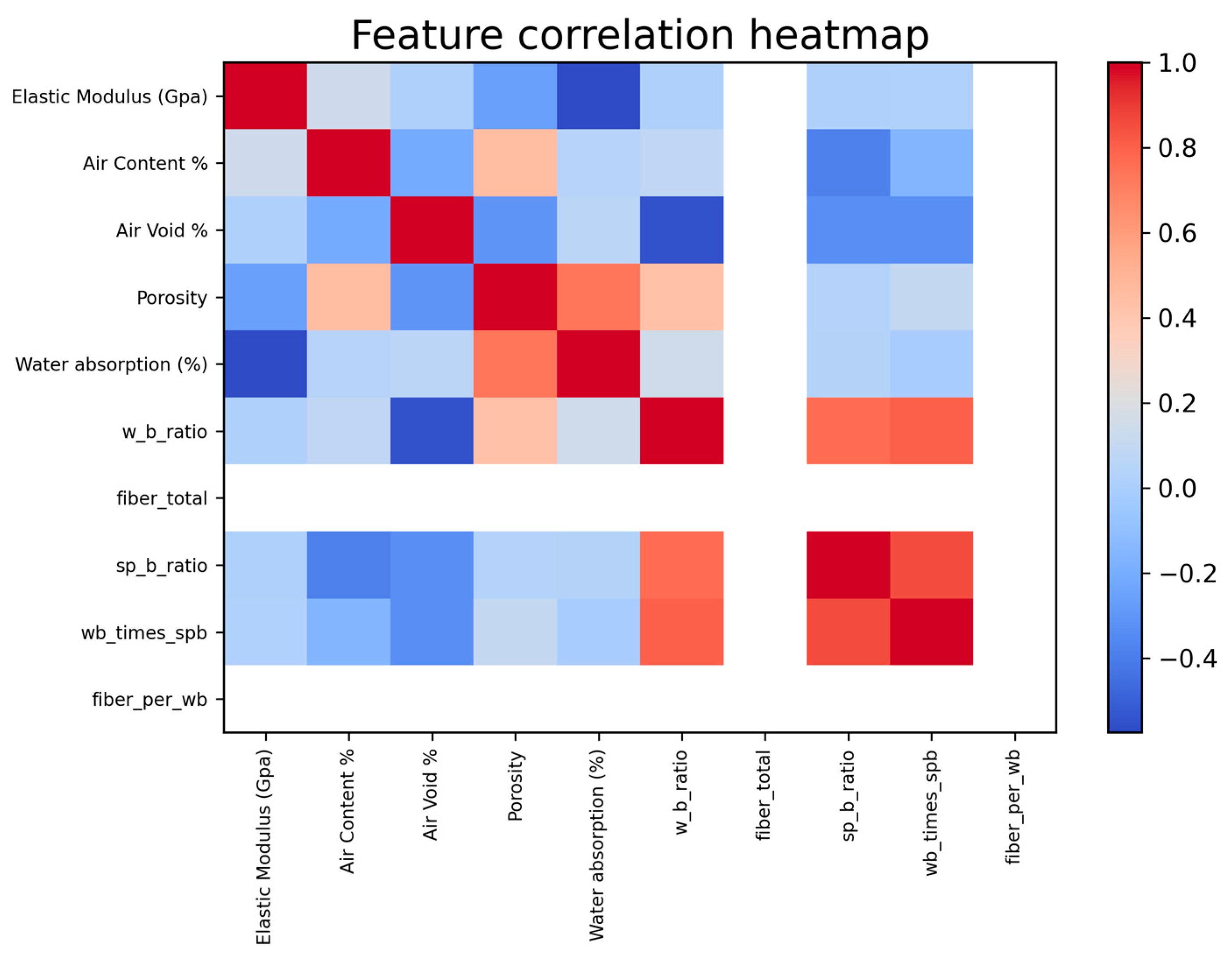
Figure 2 reports Pearson pairwise correlations among engineered inputs—elastic modulus; moisture/void descriptors; w/b, superplasticizer-to-binder ratio (sp/b); fiber-related terms; and simple interactions—showing moderate coupling within the moisture/void family and generally weak links elsewhere [33]. Together, Figure 1 (coverage/trend views) and Figure 2 (correlation screen) establish—prior to any modeling—that the dataset is both broad and internally coherent, suitable for a physics-informed (e.g., PINN-oriented) study [34]. Table 1 lists the variables retained for analysis, grouped into core predictors and mixture amount, and reports their units and distribution summaries.

2.2. Composition and Split

We track four disjoint cohorts: the full record set, samples with ≥1 target, samples with both targets, and unlabeled rows kept only for unsupervised statistics/imputation (excluded from supervised training/validation). A single split is used throughout: 80% train, 20% test; within train, a 15% validation slice is carved [31,35]. All stochastic steps (split, imputation unit, transformer fits) use seed = 42. The two supervised targets prioritize 28-day values (compressive and flexural peak); non-28-day measurements are not substituted.

2.3. Data Harmonization, Imputation, and Quality Control

Missing data follow a code-consistent policy: numerical features are completed via Gaussian copula imputation, while categorical features use an explicit missing level combined with one-hot encoding [27]. For scaling/encoding, numeric columns are standardized (StandardScaler) and categorical columns are one-hot encoded in parallel; the resulting feature blocks are horizontally concatenated to form a single design matrix. All transformations and imputation parameters are fit on the training portion only and applied unchanged to the validation/test. Reasonableness checks include range/quantile summaries of the targets, flags for near-constant predictors, and a correlation sweep (e.g., Figure 3a) to verify internal consistency. Access details and curated preprocessing artefacts (with checksums) are provided in Data Availability, ensuring exact reproducibility of record counts, splits (80/15/20, seed = 42), and descriptive summaries.
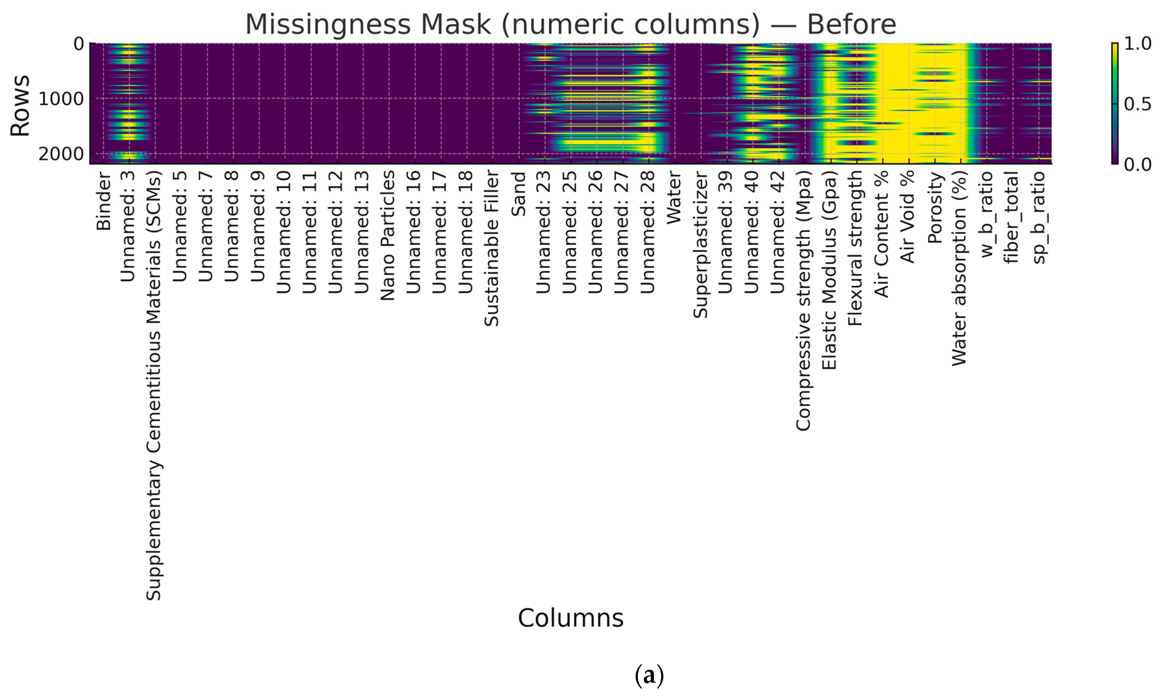
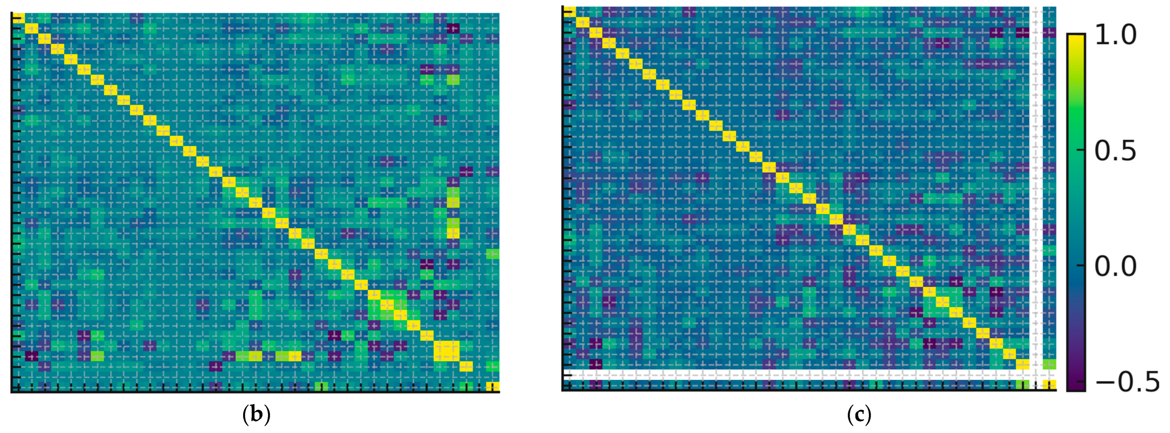
Figure 3 provides a diagnostic overview of data quality and the effect of Gaussian copula imputation. The top panel shows the missingness mask across numeric features prior to imputation, where yellow entries indicate absent values; certain columns, such as water absorption and air-related indices, exhibit substantial sparsity [13]. The bottom panels display the pairwise correlation matrices of numeric variables, with the left plot computed from the incomplete data (pairwise deletion) and the right plot obtained after copula-based completion. Before imputation, the correlation map is fragmented and noisy due to varying sample counts per pair. After imputation, correlations become smoother and more coherent, reflecting dependence structures consistent with known material interactions. This contrast highlights both the extent of missing information in raw UHPC records and the ability of copula-based methods to restore consistent multivariate relationships, thereby providing a more reliable foundation for subsequent predictive modeling.

3. Methodology

(1) The workflow first standardizes the schema and performs targeted feature engineering, forming the predictor space from the water–binder ratio, the superplasticizer–binder ratio, a total fiber descriptor, and simple interactions (water–binder × superplasticizer–binder; fiber normalized by water–binder). (2) Numerical gaps are then completed via a Gaussian copula routine that preserves marginal shapes and cross-feature dependence, while categorical gaps (e.g., cement type) are imputed by the most frequent level; categorical variables are one-hot encoded and numeric variables are standardized with statistics fit on the training split only [36,37]. (3) A single partition is adopted—80/20 train/test—and a 15% validation slice is carved from the training portion for early stopping, hyper-parameter choices, and blend weight selection [31]. (4) Modeling combines a physics-informed multi-task neural network (PINN) with Smooth-L1 supervision and learned per-task noise scales for uncertainty-weighted balancing, together with soft monotonicity regularization on input gradients (decreasing with respect to water–binder for both targets and, when valid, increasing with respect to fiber for the flexural task). (5) In parallel, a histogram-based gradient boosting regressor is trained per target; (6) final predictions are obtained by fixing a validation-selected convex combination of the PINN and tree outputs. (7) Evaluation uses MAE, RMSE, and R2 on the original scale after inverse transformation and includes residual diagnostics (prediction–actual overlays and absolute-residual-versus-prediction plots).

3.1. Data Preparation and Feature Engineering

Mixture records are harmonized without altering numeric values or units. Predictors are built from domain-standard ratios and concise interactions [38]. Let M be the set of cementitious constituents (cement, fly ash, slag, silica fume, metakaolin, nano-silica, limestone, quartz), and let B i n d e r t o t a l = m M m a s s m denote the total binder content. The water–binder ratio and superplasticizer–binder ratio are
x w b = W a t e r B i n d e r t o t a l ,                     x s p / b = S P B i n d e r t o t a l
where x w b and x s p / b are dimensionless; Water and SP are the mix water and superplasticizer dosages (mass units consistent with the source). A total fiber descriptor x f i b (as provided in the data) is retained. Two interactions are used [39] as follows:
x w b × s p / b = x w b x s p / b ,                   x f i b / w b = x f i b x w b + ε
where ε > 0 is a small constant to prevent division by zero. Numerical gaps are completed by a Gaussian copula routine: for each variable x l (index l enumerates features), estimate the empirical marginal CDF F l and map to uniforms and latent Gaussians,
u l = F l ( x l ) ,   z l = Φ 1 ( u l ) ,
where Φ is the standard normal CDF and z l is the latent Gaussianized variable. Let O and M denote the observed and missing index sets of the feature block in a row; with the latent correlation matrix Σ (projected to be positive semi-definite), missing entries are imputed by the conditional mean
E z M z O = Σ M O Σ O O 1 z O ,
and mapped back to the original scale x ^ M = F M 1 . Categorical gaps (e.g., cement type) use mode imputation. Categorical variables are then one-hot encoded; numeric variables are standardized by StandardScaler. A single split is adopted as follows: 80/20 train/test; within training, a 15% validation slice is carved for early stopping and blend weight selection. Two targets—28-day compressive and flexural peak strengths—are modeled in log space and evaluated on the original scale [40]:
y ~ j = l o g 1 + y j , z j = y ~ j μ j σ j , y ^ j = e x p y ~ ^ j 1 , j { c , f } ,
where j indexes the tasks (compressive c , flexural f ) ;   μ j ,   σ j are the training set mean and standard deviation of y ~ j ;   y ~ ^ j is the network prediction in log space; y ^ j is its back-transform.

3.2. Analytical Modeling

The physics-informed network (PINN) is a shared-trunk MLP (Linear, GELU, BatchNorm, (Dropout)) with task-specific Softplus heads in log space. Let θ denote the trainable parameters [41]. Supervision uses Smooth-L1 (Huber) on standardized residuals r j and threshold δ > 0 ,
Huber r = 1 2 r 2 , r δ , δ r δ 2 , r > δ ,
and is combined via uncertainty-weighted multi-tasking by learning per-task log variances s j =   l o g σ j , noise 2 and s = s c , s f :
L s u p θ , s = j { c , f } e x p s j E Huber r j + s j ,
Physics is injected as soft monotonicity on input gradients in log space: decreasing w.r.t. x w b for both tasks; when x f i b is present and non-degeneratje, increasing w.r.t. x f i b for the flexural task. With mini-batch B and input gradient g j , i x = y ~ ^ j / x i ,
L p h y s θ = λ p h y s E x B R e L U g c , w b x + R e L U g f , w b x + R e L U g f , f i b x ,
where λ p h y s > 0 is the physics regularization weight. The total objective is
L θ , s = L s u p + λ p h y s L p h y s + λ w d     θ   2 2
with λ wd the l 2 weight decay coefficient. Optimization uses AdamW, gradient norm clipping, and a Reduce-on-Plateau scheduler; early stopping selects the checkpoint with maximal mean validation R 2 . To reduce variance, K differently seeded models are trained and averaged as follows:
y ^ j PINN x = 1 K k = 1 K y ^ j k x ,
where K is the ensemble size and y ^ j k denotes the k -th seed’s prediction. As a non-neural comparator, a histogram-based gradient boosting regressor (HGBT) is trained per target. The FINAL predictor is a validation-selected convex blend
y ^ j final = α j y ^ j PINN + 1 α j y ^ j TREE , 0 α j 1 ,
where α j is chosen on the held-out validation slice and then fixed for the test fold.

3.3. Evaluation and Residual Analysis

All metrics are computed on the original scale after inverse transformation. Let N j be the number of test instances and y j = 1 N j n = 1 N j y j n the test set mean:
MAE j = 1 N j n = 1 N j y j n y ^ j n , RMSE j = 1 N j n = 1 N j y j n y ^ j n 2 ,
R j 2 = 1 n y j n y ^ j n 2 n y j n y j 2
Residual diagnostics include prediction–actual overlays and |residual| vs. prediction plots to assess alignment, heteroscedasticity, and tail behavior.

4. Results

4.1. Training Process

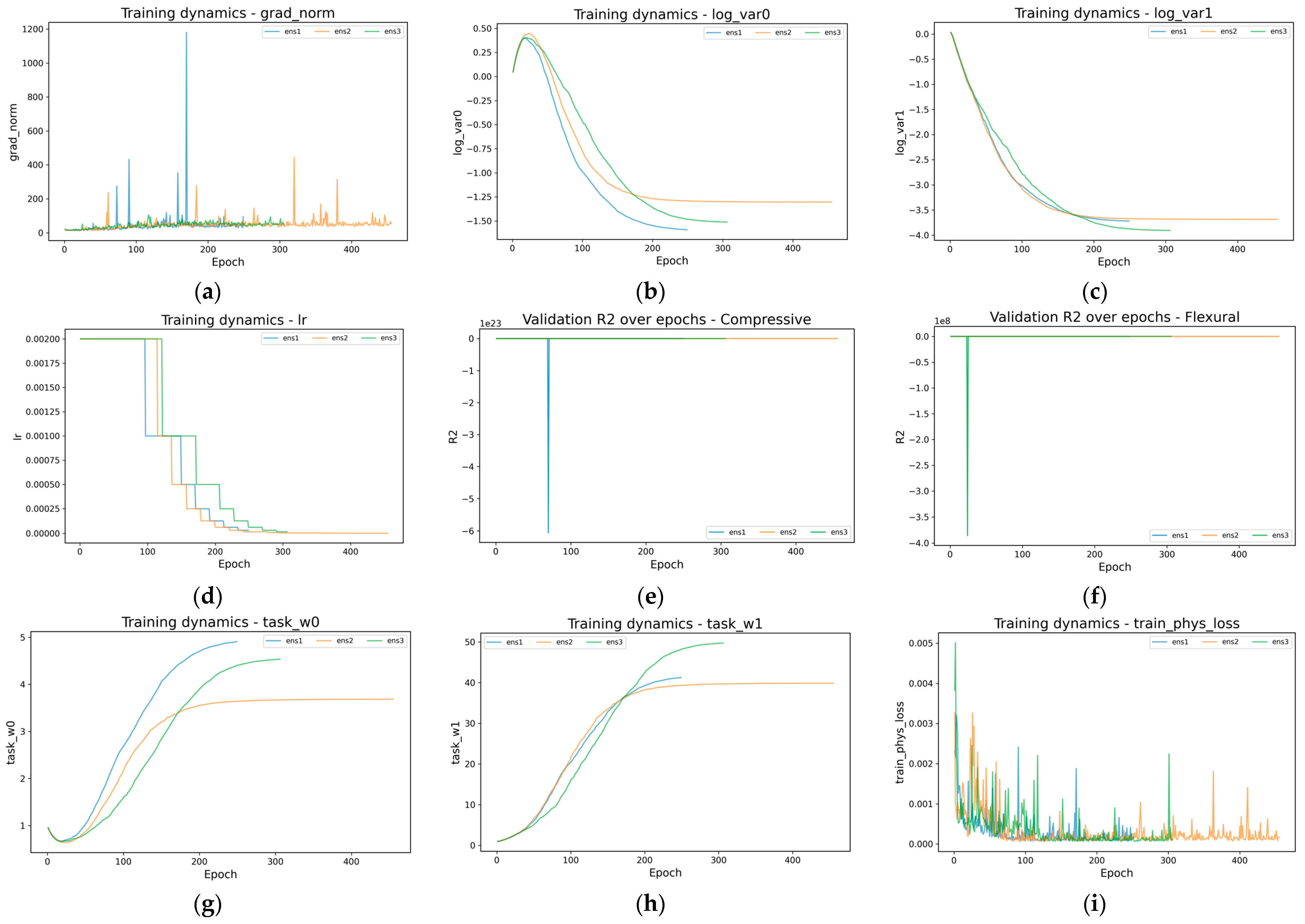
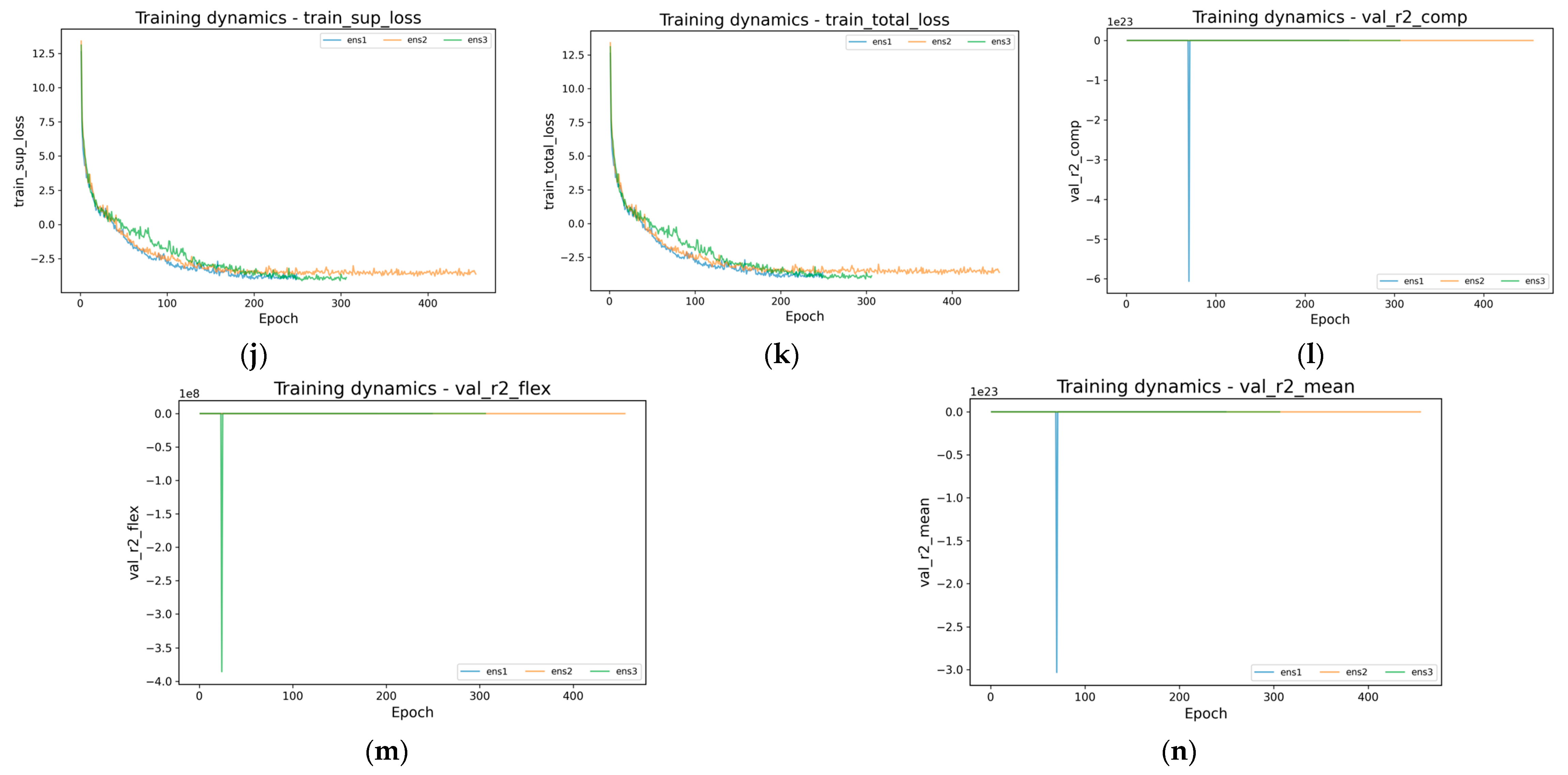
Training was monitored across three independent seeds (ens1–ens3). The supervised and total losses in Figure 4j,k exhibit the characteristic two-phase descent: a steep drop over the first ~50–100 epochs, followed by a smooth approach to a plateau [42]. The physics penalty in Figure 4i decreases by more than an order of magnitude and shows occasional spikes, consistent with one-sided inequality penalties that activate only when a constraint is violated. The learned log variances in Figure 4b,c decline monotonically—log_var0 to ≈ −1…−1.6 and log_var1 to ≈ −3…−4—while the corresponding inverse-variance weights in Figure 4g,h rise (task_w0 ≈ 5; task_w1 in the several tens range), indicating automatic rebalancing toward the lower-noise task. Gradient norms remain bounded (Figure 4a); early bursts subside as the losses flatten. Validation R2 traces for each task and for their mean (Figure 4e,f,l–n) are shown for monitoring only: large negative excursions can occur very early when predictions are still degenerate but quickly collapse into a stable band. The learning rate schedule (Figure 4d) follows a staircase decay that coincides with the onset of loss plateaus. Taken together, the tight clustering across seeds throughout Figure 4 supports optimization stability and reproducible uncertainty-weighting dynamics.

4.2. Physical Parameter Evolution

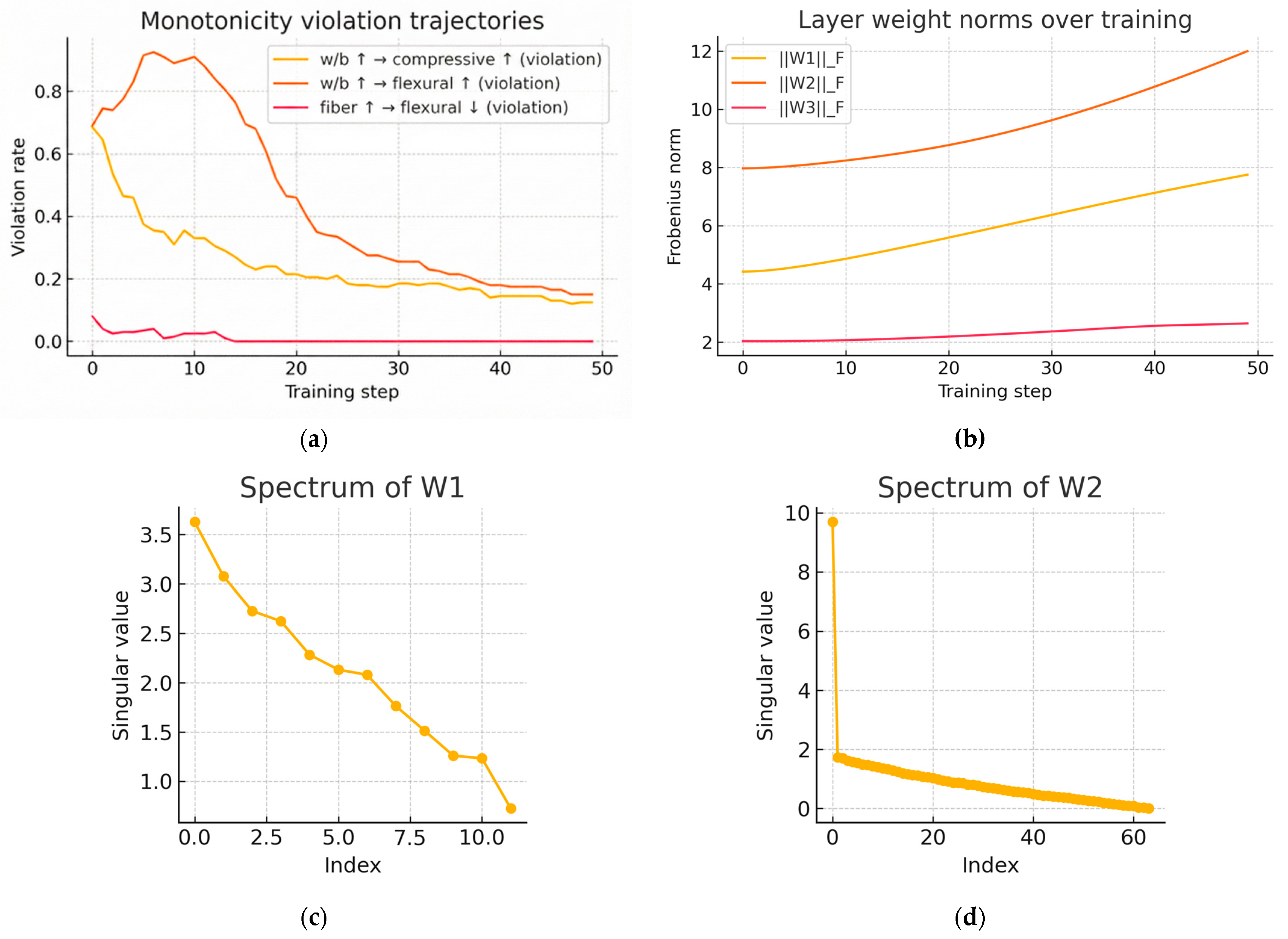
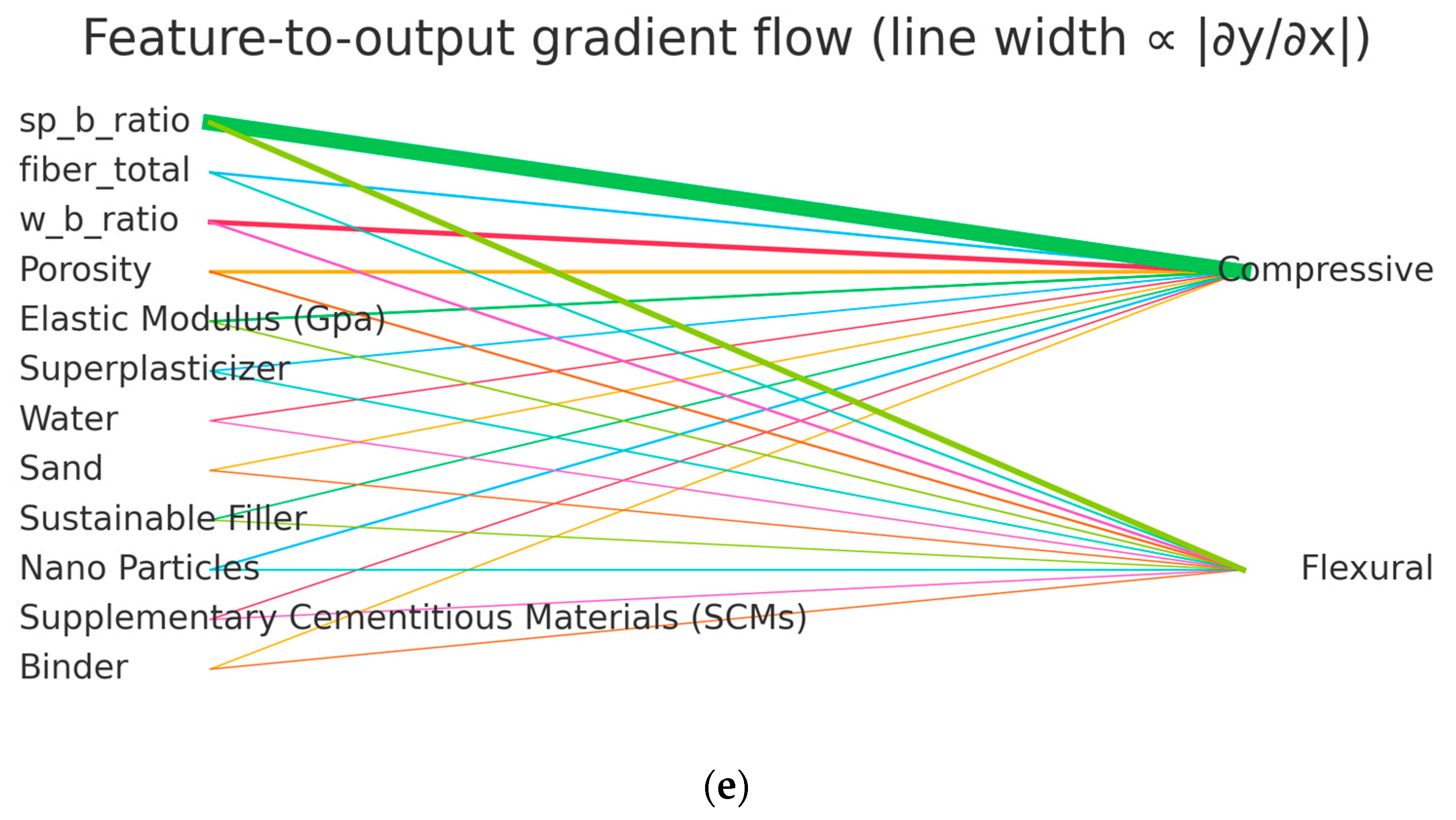
Figure 5 assembles complementary diagnostics of the physics-informed network over training. In Figure 5a, monotonicity violation rates for the priors (strength non-increasing in w/b; flexural non-decreasing in fiber) fall steadily—most notably the w/b→flexural curve from >0.8 to <0.2 by the final epochs—indicating that the soft inequality penalties are being satisfied [43]. Figure 5b shows the Frobenius norms of the layer weights growing smoothly without blow-up, consistent with controlled capacity under regularization. The singular spectra in Figure 5c,d decay rapidly, revealing a low-rank structure dominated by a few principal directions, as expected for smooth, physically constrained mappings. The gradient flow view in Figure 5e summarizes the average sensitivities (line width ∝ |∂y/∂x|): the strongest flows arise from w_b_ratio and sp_b_ratio to both targets, with fiber_total especially pronounced for the flexural head, whereas moisture/void descriptors contribute smaller magnitudes. Taken together, Figure 5 documents a training process that increasingly respects the monotonic priors, maintains stable parameter growth, learns compact representations, and concentrates sensitivity on physically salient inputs.

4.3. Model Performance

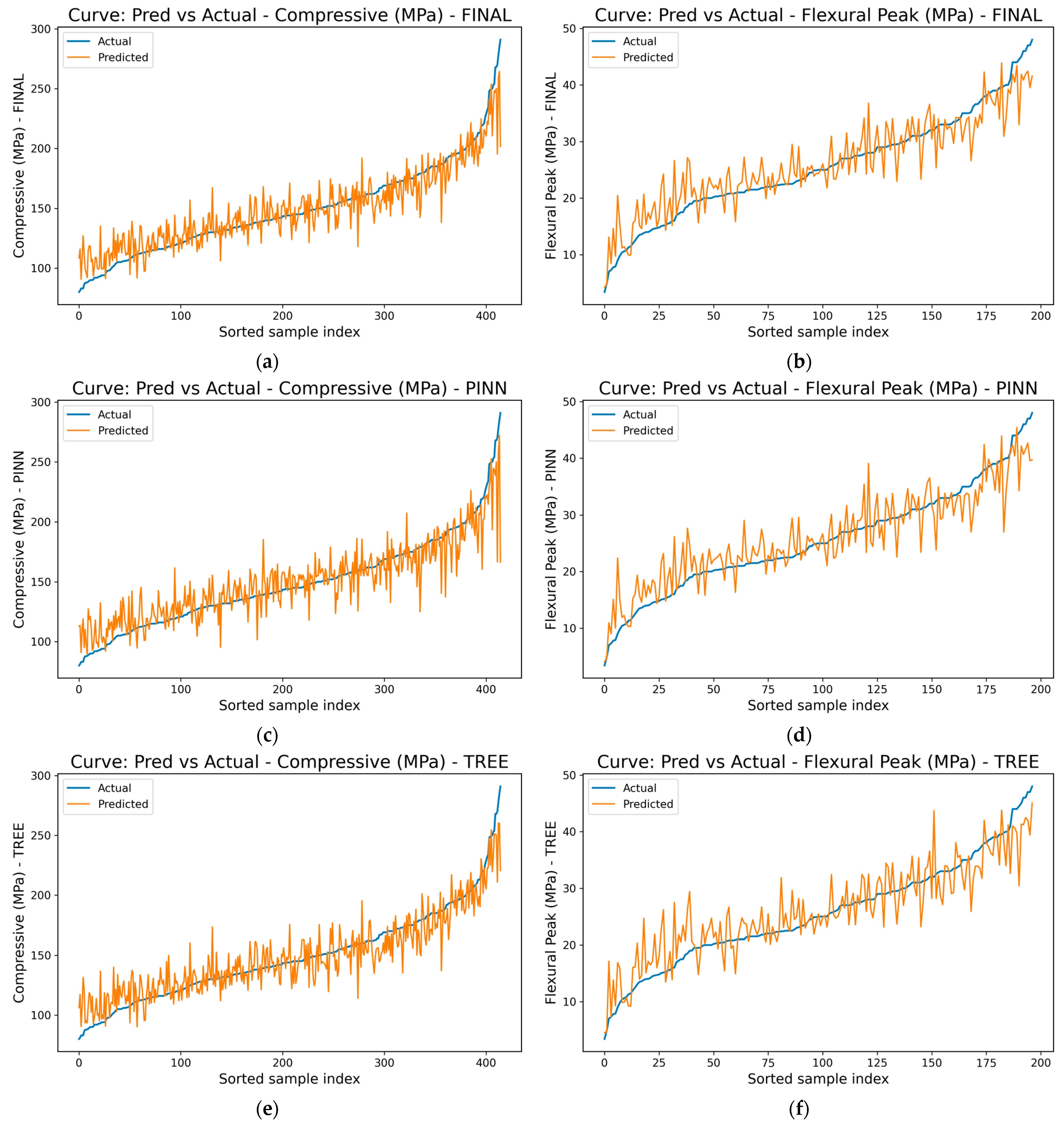
In Figure 6a–f, the orange prediction traces follow the monotonic rise in the blue ground-truth curves across the full-strength range [44]. For compressive strength, Figure 6c vs. Figure 6e shows that the PINN curve exhibits less low-frequency drift, whereas the tree curve oscillates more and occasionally overshoots near the high-strength tail. For flexural peak, both Figure 6d,f reproduce the global trend; the PINN presents a few mid-range underestimation spikes, while the tree displays higher-frequency wiggles. The FINAL blend in Figure 6a,b visibly damps these deviations—especially in the mid-strength region—yielding a smoother adherence to the ground-truth profile than either constituent model.
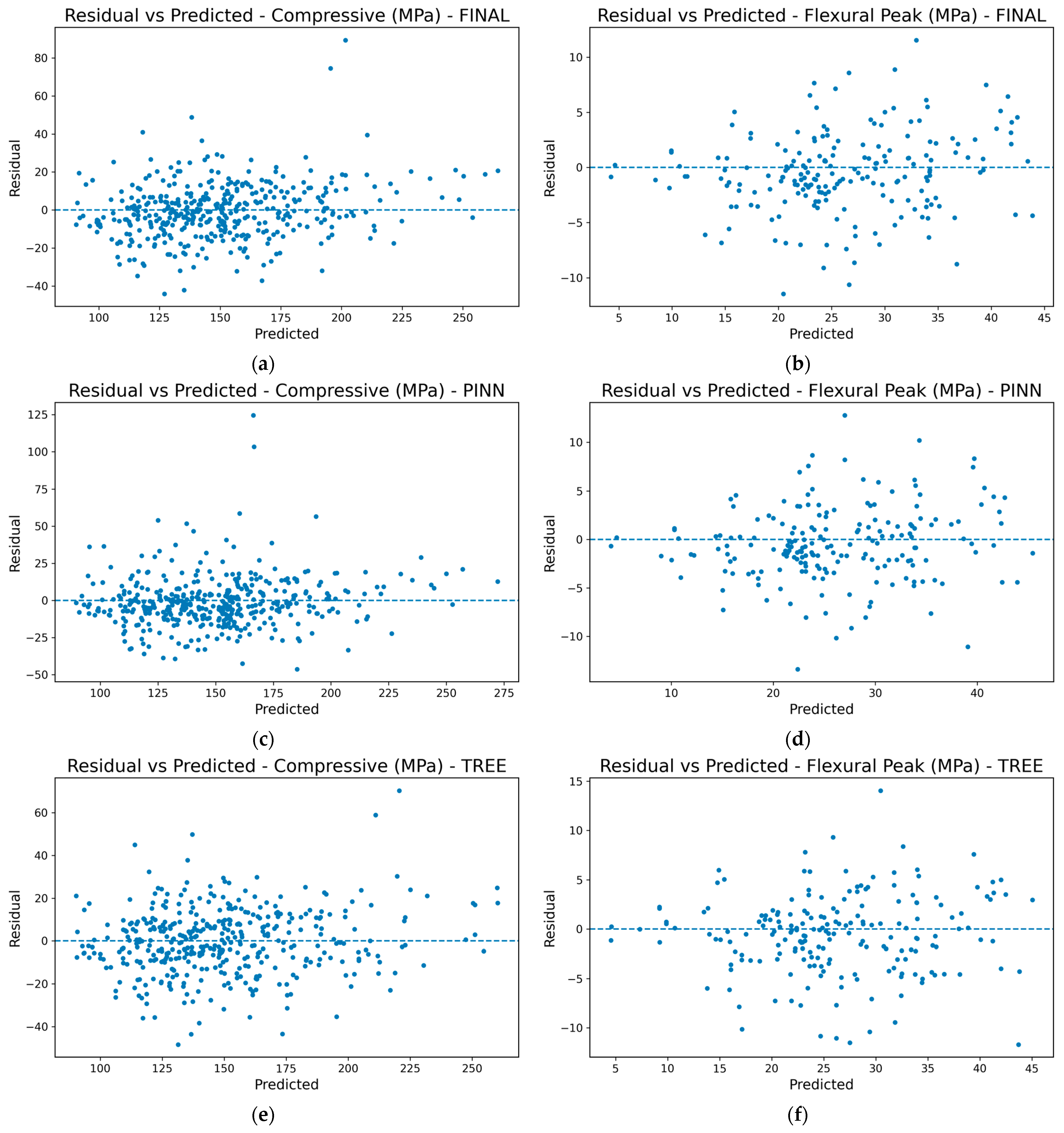
In the residual diagnostics Figure 7a–f, the clouds are approximately zero-centered with no strong curvature against predictions, indicating limited systematic bias. Scatter increases with predicted magnitude—consistent with the inverse-log back-transform and broader variance at high strength. PINN residuals Figure 7c,d are tighter with a few long-tail outliers (one large positive outlier in compressive), whereas tree residuals Figure 7e,f are more dispersed and heavy-tailed. The FINAL blend Figure 7a,b contracts these tails and flattens the mean drift, consistent with complementary error structures: the PINN provides smooth, physics-coherent trends and the tree supplies local adjustments, yielding more stable performance across the range.
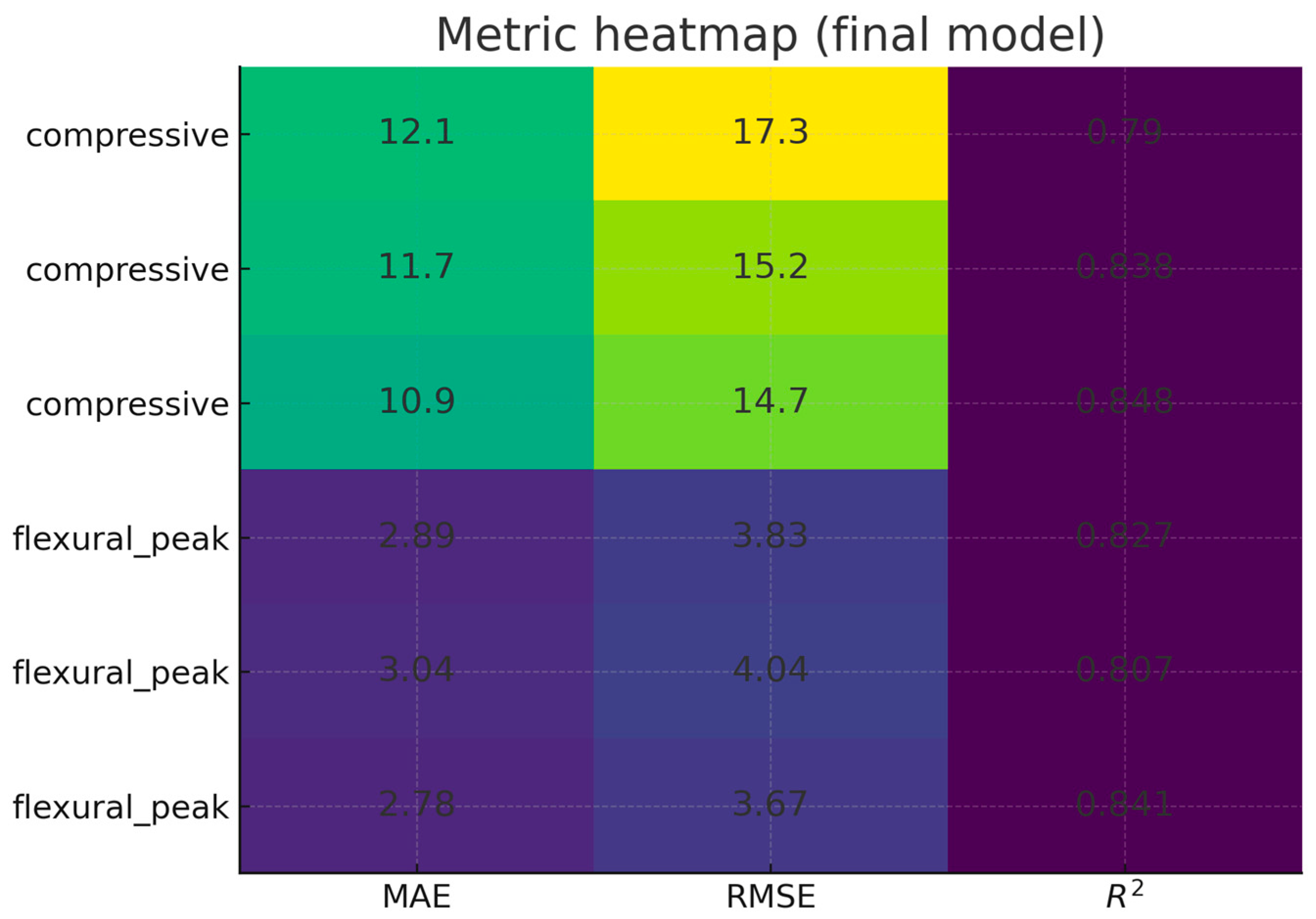
Figure 8 presents the quantitative performance of all models on the held-out test set for both compressive and flexural peak strength [45]. Each row corresponds to a specific model (histogram gradient boosting, PINN, and the convex blend), while the columns summarize three complementary metrics: mean absolute error (MAE), root-mean-square error (RMSE), and the coefficient of determination (R2). For compressive strength, the tree baseline achieves an MAE/RMSE/R2 of 12.1/17.3/0.790, the PINN reduces the errors to 11.7/15.2/0.838, and the final blend further improves to 10.9/14.7/0.848. For flexural peak strength, the corresponding results are 2.89/3.83/0.827 for the tree baseline, 3.04/4.04/0.807 for the PINN, and 2.78/3.67/0.841 for the blend. These values indicate that the convex blend consistently lowers both the MAE and RMSE compared with single models and yields the highest R2 across tasks. The improvement is particularly evident in compressive strength, where the blend gains 0.5 MPa in RMSE and 0.01 in R2 over the best standalone learner, while also providing modest but consistent gains in flexural peak prediction. This evidence supports the conclusion that combining physics-informed neural networks with tree-based learners delivers a more accurate and robust predictor for UHPC strength. Table 2 summarizes the testing results.

5. Conclusions

In this work, we developed and validated an end-to-end framework for predicting the compressive and flexural peak strength of ultra-high-performance concrete (UHPC) from heterogeneous mix records. The workflow first harmonized the mixture data into a consistent schema, then applied Gaussian copula imputation to complete missing numeric variables while preserving cross-feature dependence. Standardized ratios and interaction features—including the water–binder ratio, superplasticizer–binder ratio, and fiber descriptors—were used to form the predictor space. A physics-informed multi-task neural network (PINN) was trained with uncertainty-weighted supervision and soft monotonicity regularization on input gradients, while histogram gradient boosting (HGBT) served as a complementary baseline. Final predictions were obtained through a validation-selected convex blend of the PINN and HGBT models. Performance was quantified on held-out test sets, with multiple visualization and diagnostic tools employed to assess error distribution, parameter dynamics, and physics consistency.
(1)
Copula-based data imputation effectively completed missing values, maintained realistic correlations, and supported stable downstream learning compared with mean or median filling.
(2)
Feature engineering guided by domain ratios (w/b, sp/b, fiber descriptors) provided interpretable predictors and improved generalization by embedding known physical relationships [45].
(3)
The physics-informed PINN reduced monotonicity violations substantially over training, aligning gradients with expected physical trends and yielding smoother, low-rank representations.
(4)
The convex blend of PINN and HGBT consistently outperformed individual models, achieving an MAE/RMSE/R2 of 10.9/14.7/0.848 for compressive strength and 2.78/3.67/0.841 for flexural strength, thereby improving accuracy and robustness across tasks.
Future work will focus on extending the proposed physics-informed multi-task framework beyond compressive and flexural peak strength to additional UHPC performance indicators, such as tensile/flexural toughness, shrinkage, and durability-related properties. On the modeling side, we plan to incorporate explicit uncertainty quantification modules (e.g., deep ensembles or Bayesian variants of PINNs) to provide calibrated prediction intervals that are more suitable for design decision-making. In addition, cross-laboratory transfer and domain adaptation strategies will be explored to improve the robustness of the model under different curing regimes and testing protocols. Finally, coupling the present framework with mix-design optimization and life-cycle metrics (e.g., cost and CO2 footprint) is envisaged to support the development of greener and more economical UHPC mixtures [46].

Author Contributions

Conceptualization, L.Y. and P.L.; Methodology, L.Y. and P.L.; Software, L.Y.; Validation, L.Y. and Y.Y.; Investigation, L.Y. and F.Y.; Resources, L.Y. and F.Y.; Data curation, L.Y., Y.Y. and F.Y.; Writing—original draft, L.Y.; Writing—review & editing, Y.Y. and X.F.; Visualization, P.L. and X.F.; Supervision, P.L. and X.F. All authors have read and agreed to the published version of the manuscript.

Funding

This research received no external funding.

Data Availability Statement

Data are contained within the article.

Conflicts of Interest

Author Fan Yang was employed by the company Shaanxi Construction Engineering Group No. 5 Construction Co., Ltd. The remaining authors declare that the research was conducted in the absence of any commercial or financial relationships that could be construed as a potential conflict of interest.

References

  1. Du, J.; Meng, W.; Khayat, K.H.; Bao, Y.; Guo, P.; Lyu, Z.; Abu-Obeidah, A.; Nassif, H.; Wang, H. New development of ultra-high-performance concrete (UHPC). Compos. Part B Eng. 2021, 224, 109220. [Google Scholar] [CrossRef]
  2. Azmee, N.M.; Shafiq, N. Ultra-high performance concrete: From fundamental to applications. Case Stud. Constr. Mater. 2018, 9, e00197. [Google Scholar] [CrossRef]
  3. Yoo, D.-Y.; Yoon, Y.-S. A review on structural behavior, design, and application of ultra-high-performance fiber-reinforced concrete. Int. J. Concr. Struct. Mater. 2016, 10, 125–142. [Google Scholar] [CrossRef]
  4. Mousavinezhad, S.; Gonzales, G.J.; Toledo, W.K.; Garcia, J.M.; Newtson, C.M.; Allena, S. A comprehensive study on non-proprietary ultra-high-performance concrete containing supplementary cementitious materials. Materials 2023, 16, 2622. [Google Scholar] [CrossRef]
  5. Abellán-García, J.; Carvajal-Muñoz, J.S.; Ramírez-Munévar, C. Application of ultra-high-performance concrete as bridge pavement overlays: Literature review and case studies. Constr. Build. Mater. 2024, 410, 134221. [Google Scholar] [CrossRef]
  6. Liao, J.; Yang, K.Y.; Zeng, J.-J.; Quach, W.-M.; Ye, Y.-Y.; Zhang, L. Compressive behavior of FRP-confined ultra-high performance concrete (UHPC) in circular columns. Eng. Struct. 2021, 249, 113246. [Google Scholar] [CrossRef]
  7. Yu, R.; Spiesz, P.; Brouwers, H. Mix design and properties assessment of ultra-high performance fibre reinforced concrete (UHPFRC). Cem. Concr. Res. 2014, 56, 29–39. [Google Scholar] [CrossRef]
  8. Nguyen, N.-H.; Abellán-García, J.; Lee, S.; Garcia-Castano, E.; Vo, T.P. Efficient estimating compressive strength of ultra-high performance concrete using XGBoost model. J. Build. Eng. 2022, 52, 104302. [Google Scholar] [CrossRef]
  9. Zeng, J.-J.; Zeng, W.-B.; Ye, Y.-Y.; Liao, J.; Zhuge, Y.; Fan, T.-H. Flexural behavior of FRP grid reinforced ultra-high-performance concrete composite plates with different types of fibers. Eng. Struct. 2022, 272, 115020. [Google Scholar] [CrossRef]
  10. ASTM C109; Standard Test Method for Compressive Strength of Hydraulic Cement Mortars. ASTM International: West Conshohocken, PA, USA, 2024.
  11. ASTM C1609; Standard Test Method for Flexural Performance of Fiber-Reinforced Concrete. ASTM International: West Conshohocken, PA, USA, 2019.
  12. ASTM C1012; Standard Test Method for Length Change of Hydraulic-Cement Mortars Exposed to a Sulfate Solution. ASTM International: West Conshohocken, PA, USA, 2024.
  13. Mahjoubi, S.; Barhemat, R.; Meng, W.; Bao, Y. AI-guided auto-discovery of low-carbon cost-effective ultra-high performance concrete (UHPC). Resour. Conserv. Recycl. 2023, 189, 106741. [Google Scholar] [CrossRef]
  14. Wang, D.; Shi, C.; Wu, Z.; Xiao, J.; Huang, Z.; Fang, Z. A review on ultra high performance concrete: Part II. Hydration, microstructure and properties. Constr. Build. Mater. 2015, 96, 368–377. [Google Scholar] [CrossRef]
  15. Behnood, A.; Golafshani, E.M. Predicting the compressive strength of silica fume concrete using hybrid artificial neural network with multi-objective grey wolves. J. Clean. Prod. 2018, 202, 54–64. [Google Scholar] [CrossRef]
  16. Bolbolvand, M.; Tavakkoli, S.M.; Alaee, F.J. Prediction of compressive and flexural strengths of ultra-high-performance concrete (UHPC) using machine learning for various fiber types. Constr. Build. Mater. 2025, 493, 143135. [Google Scholar] [CrossRef]
  17. Zhang, Y.; Yang, Q. A survey on multi-task learning. IEEE Trans. Knowl. Data Eng. 2021, 34, 5586–5609. [Google Scholar] [CrossRef]
  18. Wen, C.; Zhang, P.; Wang, J.; Hu, S. Influence of fibers on the mechanical properties and durability of ultra-high-performance concrete: A review. J. Build. Eng. 2022, 52, 104370. [Google Scholar] [CrossRef]
  19. Gong, J.; Ma, Y.; Fu, J.; Hu, J.; Ouyang, X.; Zhang, Z.; Wang, H. Utilization of fibers in ultra-high performance concrete: A review. Compos. Part B Eng. 2022, 241, 109995. [Google Scholar] [CrossRef]
  20. Onyelowe, K.C.; Hanandeh, S.; Ulloa, N.; Barba-Vera, R.; Moghal, A.A.B.; Ebid, A.M.; Arunachalam, K.P.; Ur Rehman, A. Developing machine learning frameworks to predict mechanical properties of ultra-high performance concrete mixed with various industrial byproducts. Sci. Rep. 2025, 15, 24791. [Google Scholar] [CrossRef]
  21. Karniadakis, G.E.; Kevrekidis, I.G.; Lu, L.; Perdikaris, P.; Wang, S.; Yang, L. Physics-informed machine learning. Nat. Rev. Phys. 2021, 3, 422–440. [Google Scholar] [CrossRef]
  22. Zhao, Y.; Udell, M. gcimpute: A package for missing data imputation. J. Stat. Softw. 2024, 108, 1–27. [Google Scholar] [CrossRef]
  23. Aghajanzadeh, E.; Bahraini, T.; Mehrizi, A.H.; Yazdi, H.S. Task weighting based on particle filter in deep multi-task learning with a view to uncertainty and performance. Pattern Recognit. 2023, 140, 109587. [Google Scholar] [CrossRef]
  24. Zhao, J.; Zhang, H.; Wang, Y.; Zhai, Y.; Yang, Y. Deep Isotonic Embedding Network: A flexible Monotonic Neural Network. Neural Netw. 2024, 171, 457–465. [Google Scholar] [CrossRef]
  25. Arrieta, A.B.; Díaz-Rodríguez, N.; Del Ser, J.; Bennetot, A.; Tabik, S.; Barbado, A.; García, S.; Gil-López, S.; Molina, D.; Benjamins, R. Explainable Artificial Intelligence (XAI): Concepts, taxonomies, opportunities and challenges toward responsible AI. Inf. Fusion 2020, 58, 82–115. [Google Scholar] [CrossRef]
  26. Rudin, C. Stop explaining black box machine learning models for high stakes decisions and use interpretable models instead. Nat. Mach. Intell. 2019, 1, 206–215. [Google Scholar] [CrossRef] [PubMed]
  27. Zhao, Y.; Udell, M. Missing value imputation for mixed data via gaussian copula. In Proceedings of the 26th ACM SIGKDD International Conference on Knowledge Discovery & Data Mining, San Diego, CA, USA, 23–27 August 2020; pp. 636–646. [Google Scholar] [CrossRef]
  28. Friedman, J.H. Greedy function approximation: A gradient boosting machine. Ann. Stat. 2001, 29, 1189–1232. [Google Scholar] [CrossRef]
  29. Peng, R.D. Reproducible research in computational science. Science 2011, 334, 1226–1227. [Google Scholar] [CrossRef] [PubMed]
  30. Sandve, G.K.; Nekrutenko, A.; Taylor, J.; Hovig, E. Ten simple rules for reproducible computational research. PLoS Comput. Biol. 2013, 9, e1003285. [Google Scholar] [CrossRef]
  31. Kashem, A.; Karim, R.; Malo, S.C.; Das, P.; Datta, S.D.; Alharthai, M. Hybrid data-driven approaches to predicting the compressive strength of ultra-high-performance concrete using SHAP and PDP analyses. Case Stud. Constr. Mater. 2024, 20, e02991. [Google Scholar] [CrossRef]
  32. Zhang, Y.; Ren, W.; Chen, Y.; Mi, Y.; Lei, J.; Sun, L. Predicting the compressive strength of high-performance concrete using an interpretable machine learning model. Sci. Rep. 2024, 14, 28346. [Google Scholar] [CrossRef]
  33. Aylas-Paredes, B.K.; Han, T.; Neithalath, A.; Huang, J.; Goel, A.; Kumar, A.; Neithalath, N. Data driven design of ultra high performance concrete prospects and application. Sci. Rep. 2025, 15, 9248. [Google Scholar] [CrossRef]
  34. Wang, X.Q.; Chow, C.L.; Lau, D. Multiscale perspectives for advancing sustainability in fiber reinforced ultra-high performance concrete. Npj Mater. Sustain. 2024, 2, 13. [Google Scholar] [CrossRef]
  35. Sun, C.; Wang, K.; Liu, Q.; Wang, P.; Pan, F. Machine-learning-based comprehensive properties prediction and mixture design optimization of ultra-high-performance concrete. Sustainability 2023, 15, 15338. [Google Scholar] [CrossRef]
  36. Lyngdoh, G.A.; Zaki, M.; Krishnan, N.A.; Das, S. Prediction of concrete strengths enabled by missing data imputation and interpretable machine learning. Cem. Concr. Compos. 2022, 128, 104414. [Google Scholar] [CrossRef]
  37. Thai, H.-T. Machine learning for structural engineering: A state-of-the-art review. In Structures; Elsevier: Amsterdam, The Netherlands, 2022; pp. 448–491. [Google Scholar] [CrossRef]
  38. Alabduljabbar, H.; Khan, M.; Awan, H.H.; Eldin, S.M.; Alyousef, R.; Mohamed, A.M. Predicting ultra-high-performance concrete compressive strength using gene expression programming method. Case Stud. Constr. Mater. 2023, 18, e02074. [Google Scholar] [CrossRef]
  39. Fan, D.; Chen, Z.; Cao, Y.; Liu, K.; Yin, T.; Lv, X.-S.; Lu, J.-X.; Zhou, A.; Poon, C.S.; Yu, R. Intelligent predicting and monitoring of ultra-high-performance fiber reinforced concrete composites—A review. Compos. Part A Appl. Sci. Manuf. 2025, 188, 108555. [Google Scholar] [CrossRef]
  40. Nithurshan, M.; Elakneswaran, Y. A systematic review and assessment of concrete strength prediction models. Case Stud. Constr. Mater. 2023, 18, e01830. [Google Scholar] [CrossRef]
  41. Shaban, W.M.; Elbaz, K.; Zhou, A.; Shen, S.-L. Physics-informed deep neural network for modeling the chloride diffusion in concrete. Eng. Appl. Artif. Intell. 2023, 125, 106691. [Google Scholar] [CrossRef]
  42. Wirz, C.D.; Sutter, C.; Demuth, J.L.; Mayer, K.J.; Chapman, W.E.; Cains, M.G.; Radford, J.; Przybylo, V.; Evans, A.; Martin, T. Increasing the reproducibility and replicability of supervised AI/ML in the Earth systems science by leveraging social science methods. Earth Space Sci. 2024, 11, e2023EA003364. [Google Scholar] [CrossRef]
  43. Li, S.; Jensen, O.M.; Yu, Q. Influence of steel fiber content on the rate-dependent flexural performance of ultra-high performance concrete with coarse aggregates. Constr. Build. Mater. 2022, 318, 125935. [Google Scholar] [CrossRef]
  44. Elshaarawy, M.K.; Alsaadawi, M.M.; Hamed, A.K. Machine learning and interactive GUI for concrete compressive strength prediction. Sci. Rep. 2024, 14, 16694. [Google Scholar] [CrossRef]
  45. Nguyen, M.H.; Nguyen, T.-A.; Ly, H.-B. Ensemble XGBoost schemes for improved compressive strength prediction of UHPC. In Structures; Elsevier: Amsterdam, The Netherlands, 2023; p. 105062. [Google Scholar] [CrossRef]
  46. Mostafaei, H.; Kelishadi, M.; Bahmani, H.; Wu, C.; Ghiassi, B. Development of sustainable HPC using rubber powder and waste wire: Carbon footprint analysis, mechanical and microstructural properties. Eur. J. Environ. Civ. Eng. 2025, 29, 399–420. [Google Scholar] [CrossRef]
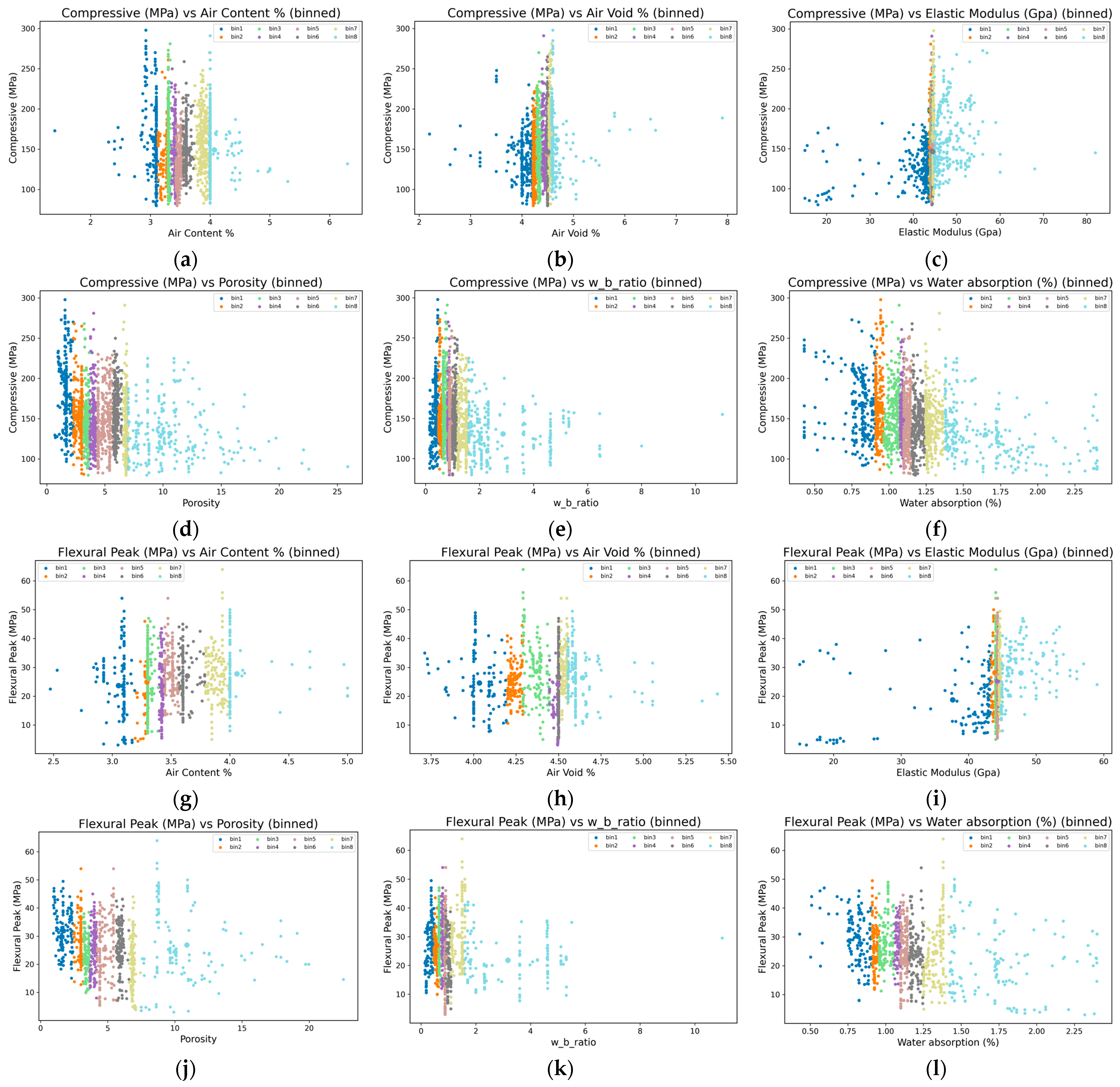
Figure 1. Univariate binned relations and rank overlays: (af) Compressive strength vs. air content (%), air void (%), elastic modulus (GPa), porosity, w_b_ratio, water absorption (%); (gl) flexural peak strength vs. the same six covariates; (m,n) rank overlay views for compressive and flexural: each covariate is rescaled to its [0, 1] rank and over-plotted to visualize distributional tendencies across quantiles.
Buildings 15 04243 g001aBuildings 15 04243 g001b
Figure 2. Feature correlation heatmap. Pairwise Pearson correlations among engineered inputs—elastic modulus, air content (%), air void (%), porosity, water absorption (%), w_b_ratio, sp_b_ratio, fiber_total, and simple interactions.
Buildings 15 04243 g002
Figure 3. Missingness structure and correlation preservation before and after copula-based imputation: (a) Missingness mask for numeric features before imputation (yellow = missing, purple = observed). (b) Pairwise Pearson correlation heatmap computed on incomplete data (pairwise deletion). (c) Correlation heatmap after Gaussian copula imputation on the completed dataset, showing the original block structure largely preserved with reduced noise.
Buildings 15 04243 g003aBuildings 15 04243 g003b
Figure 4. (a) Gradient norm per epoch for three seeds (ens1–ens3). (b) Log variance for task 0 (compressive) and (c) for task 1 (flexural) learned by the uncertainty module. (d) Learning rate schedule. (e) Validation R2—compressive (streaming computation). (f) Validation R2—flexural (streaming computation). (g,h) Learned task weights w 0 , w 1 . (i) Physics constraint loss. (j) Supervised loss. (k) Total loss. (l) Validation R2—compressive (batched computation). (m) Validation R2—flexural (batched computation). (n) Mean validation R2 across the two targets.
Buildings 15 04243 g004aBuildings 15 04243 g004b
Figure 5. PINN parameter dynamics, spectral characteristics, and gradient-based feature sensitivities: (a) Monotonicity violation rate vs. training step for three priors: w/b↑→compressive↑ (violation), w/b↑→flexural↑ (violation), fiber↑→flexural↓ (violation); lower is better. (b) Frobenius norms of layer weights ‖W1‖_F, ‖W2‖_F, ‖W3‖_F over training. (c) Final singular-value spectrum of W1. (d) Final singular-value spectrum of W2. (e) Gradient-based feature sensitivities (line width ∝ mean |∂y/∂x| on validation).
Buildings 15 04243 g005aBuildings 15 04243 g005b
Figure 6. Predicted–actual curves on the held-out set: (a) Stacked FINAL predictor vs. actual—compressive strength; (b) stacked FINAL predictor vs. actual—flexural peak strength. (c) PINN-only vs. actual—compressive; (d) PINN-only vs. actual—flexural. (e) Tree-only vs. actual—compressive; (f) tree-only vs. actual—flexural. Curves are drawn against the sample index after sorting by the ground-truth target (blue: actual; orange: predicted).
Buildings 15 04243 g006
Figure 7. Residual-versus-predicted diagnostics: (a) Residual vs. predicted—FINAL, compressive; (b) residual vs. predicted—FINAL, flexural. (c) Residual vs. predicted—PINN, compressive; (d) residual vs. predicted—PINN, flexural. (e) Residual vs. predicted—tree, compressive; (f) residual vs. predicted—tree, flexural. Dashed horizontal lines mark zero residual.
Buildings 15 04243 g007
Figure 8. Metric heatmap for the final predictor on held-out UHPC mixes.
Buildings 15 04243 g008
Table 1. Variable dictionary and descriptive statistics of the UHPC dataset.
CategoryVariable Unit Type Valid N Missing (%) Median
[Q1–Q3]
Range
(min–max)
P5–P95Mean ± SD Skew/
Kurt
Core predictorsAir content (%)%Num3998.223.42 [3.01–4]1.4–6.32.39–5.033.580 ± 0.9520.436/0.698
Air void (%)%Num2998.684.5 [3.7–5.5]2.2–7.92.64–6.564.524 ± 1.3220.44/0.020
Elastic modulus (GPa)GPaNum26188.0844.26 [41.5–49.672]15–8226–5544.401 ± 8.623−0.206
Porosity (—)Num23989.084.4 [2.15–9.45]0.69–25.891.069–16.526.223 ± 5.1561.21/0.951
Water absorption (%)%Num2199.041.1 [0.82–1.72]0.43–2.40.58–2.371.260 ± 0.5600.665/−0.526
sp_b_ratioNum20327.170.15 [0.075–0.206]0–1.833330.0283–0.4990.1817 ± 0.1853.97/24
w_b_ratioNum20327.170.878 [0.653–1.200]0.142857–110.36–2.6631.114 ± 0.9313.7/20.9
Mixture amountsCement (kg/m3)kg/m3Num21880.05197.1 [133.425–227.25]0–617.6470–288180.566 ± 89.3290.29/3.06
Sand (kg/m3)kg/m3Num21880.05960 [820.8–1056]0–1994310–1250902.747 ± 291.326−0.450
Water (kg/m3)kg/m3Num21880.05183.26 [166.972–211.5]110–355.147147–299.52194.591 ± 42.8011.38/1.97
Median [Q1–Q3]—median with interquartile range (25th–75th percentiles); robust summary of the central tendency and spread. P5–P95—5th to 95th percentile interval; reduces the influence of extreme outliers and indicates the typical operating range. Mean ± SD—arithmetic mean and standard deviation. Skew/Kurt—sample skewness and kurtosis (excess kurtosis if not otherwise specified); they describe asymmetry and tail heaviness of the distribution.
Table 2. Model performance.
TargetModelMAERMSER2Test_n
compressivePINN12.0517.290.79415
Tree11.7115.180.84415
FinalBlend10.8614.680.85415
flexural_peakPINN2.893.830.83197
Tree3.044.040.81197
FinalBlend2.783.670.84197
Disclaimer/Publisher’s Note: The statements, opinions and data contained in all publications are solely those of the individual author(s) and contributor(s) and not of MDPI and/or the editor(s). MDPI and/or the editor(s) disclaim responsibility for any injury to people or property resulting from any ideas, methods, instructions or products referred to in the content.