Effect of Freeze–Thaw Cycles on Bond Properties at the FRP-Concrete Interface: Experimental Evaluation and Machine Learning Prediction

Abstract

Fiber-reinforced polymer (FRP)–concrete bonding is widely adopted for structural strengthening, yet its durability is highly vulnerable to freeze–thaw (FT) degradation. This study combines experimental testing with interpretable machine learning (ML) to reveal the degradation mechanism and predict the interfacial behavior of FRP–concrete systems under FT exposure. Single-lap shear tests showed that all specimens failed through interfacial debonding accompanied by partial concrete peeling. The ultimate bond strength decreased by 6.0–18.5%, and the peak shear stress dropped by 53–80%, indicating a pronounced loss of ductility and adhesion. To extend the analysis, experimental data were integrated with literature datasets, and three ensemble ML algorithms—AdaBoost, Random Forest (RF), and Extreme Gradient Boosting (XGBoost)—were employed to predict key bond–slip parameters including ultimate bond strength, local maximum bond stress, slip values, and interfacial fracture energy. Among them, XGBoost achieved the highest predictive accuracy, with R² values exceeding 0.94 for most output parameters and consistently low RMSE values. Shapley Additive exPlanations (SHAP) and Partial Dependence Plots (PDPs) further identified adhesive tensile strength, fiber modulus, FRP thickness, and concrete strength as dominant factors and defined their optimal ranges. The findings offer a scientific foundation for evaluating and predicting the long-term bond durability of FRP–concrete systems and support the development of reliable reinforcement strategies for infrastructure in cold and severe environments.

1. Introduction

Fiber-reinforced polymer (FRP) composites have been widely adopted for the strengthening and rehabilitation of reinforced concrete (RC) structures owing to their high tensile strength, low weight, and excellent corrosion resistance [1,2,3,4]. The overall performance of FRP-strengthened systems is fundamentally governed by the bond behavior at the FRP–concrete interface, which controls the efficiency of stress transfer and, consequently, dictates the load-bearing capacity and long-term durability of the strengthened member [5,6]. However, when exposed to aggressive service environments, the integrity of the FRP–concrete interface can deteriorate significantly. In cold or seasonally fluctuating regions, repeated freeze–thaw (FT) cycles represent one of the most severe environmental stressors, progressively degrading the interfacial bond performance and consequently reducing structural integrity and service life [7].

Extensive research has been conducted to explore the degradation of the FRP–concrete bond under FT exposure. Jiang et al. [8] experimentally demonstrated that repeated FT cycles led to significant reductions in bond strength and interfacial stiffness due to microcrack accumulation in the interfacial transition zone (ITZ). Zhang et al. [9] further revealed that sulfate–FT coupling accelerated interfacial degradation and reduced the effective bonding area, while Zhang et al. [10] confirmed that both static and dynamic bond capacities declined markedly with increasing FT cycles. Wang and Petrů [11] observed that ice-induced stresses severely reduced the fracture energy and shifted the failure mode toward adhesive debonding. Although these studies provide valuable insights, the mechanisms of FT-induced interfacial degradation remain insufficiently clarified and often lack a consistent modeling framework. In addition, recent works have explored performance-based predictive models for FRP-strengthened systems under harsh environmental conditions [12,13], but most of these focus solely on ultimate bond strength, neglecting the evolution of key bond–slip parameters such as peak shear stress, slip capacity, and fracture energy. Furthermore, current models are often built on limited datasets and simplified assumptions, resulting in reduced reliability when applied under coupled environmental–mechanical conditions.

In recent years, machine learning (ML) techniques have been increasingly adopted in concrete engineering to enhance predictive accuracy, computational efficiency, and model interpretability [14,15,16,17,18]. For FRP–concrete systems, data-driven models have demonstrated strong potential in capturing nonlinear relationships among geometric, material, and environmental factors, often outperforming traditional empirical formulations. Zhou et al. [19] developed an explicit neural network model trained on a large experimental dataset, achieving high accuracy and generalizability in predicting interfacial bond strength. Chen et al. [20] proposed an ensemble learning framework to improve robustness and minimize prediction errors across diverse test conditions. Similarly, Zhang et al. [21] constructed ML-based regression models capable of accurately estimating ultimate bond strength, fracture energy, and stiffness. Kumar et al. [22] further introduced a user-friendly graphical interface based on ML, enabling efficient bond strength prediction under variable exposure conditions. Su et al. [23] evaluated multiple ML algorithms and optimized model selection for FRP–concrete bond strength prediction, while Zhu et al. [24] employed SHAP-based explainable ML methods to quantify the relative importance of input variables and enhance interpretability. In addition, Qu et al. [25] proposed a GAN–ANN hybrid model to address small-sample limitations in FRP–concrete datasets, providing a viable solution for rare-condition modeling. Ge et al. [26] utilized metaheuristic algorithm-optimized ML frameworks, demonstrating superior performance in bond strength prediction under high-temperature environments. Despite these advancements, most existing studies remain limited to predicting the ultimate bond strength, lacking comprehensive modeling of the full bond–slip evolution at the FRP–concrete interface, and failing to adequately account for the coupled degradation effects under environmental exposures, particularly freeze–thaw cycles.

Most existing models, whether empirical or data-driven, focus solely on predicting ultimate bond strength under ambient conditions, without capturing the evolution of bond–slip behavior or the degradation of key interfacial parameters under FT exposure. The environmental sensitivity of peak shear stress, slip capacity, and fracture energy remains insufficiently quantified, limiting accurate durability assessments. To address this gap, the present study integrates experimental investigation and machine learning (ML) modeling to systematically evaluate and predict the degradation of FRP–concrete interfacial properties under FT cycles. A series of single-lap shear tests were conducted to quantify changes in bond strength, slip response, and fracture energy across different FT cycles, enabling a comprehensive understanding of bond deterioration trends. Based on the experimental dataset, interpretable ML models were developed to predict key bond–slip parameters and to identify the relative influence of geometric, material, and environmental variables. Unlike previous studies that emphasize only ultimate strength, this work establishes a generalized, data-driven framework for assessing and forecasting the environmental sensitivity of interface performance in cold-region applications.

2. Experimental Program

2.1. Material Properties and Specimen Setup

This study systematically investigated the evolution of bond performance at the FRP–concrete interface under the influence of freeze–thaw cycles, using concrete with an average 28-day compressive strength of 55.5 Mpa as the substrate. To perform single-lap shear tests, standard concrete prism specimens were designed and fabricated with dimensions of 100 mm (width) × 100 mm (height) × 300 mm (length). The interface was strengthened using unidirectional carbon fiber-reinforced polymer (CFRP) sheets, which exhibited a tensile strength of 3731.0 Mpa, an elastic modulus of 238 GPa, and a nominal thickness of 0.167 mm. The structural adhesive was a two-component epoxy resin used as the CFRP impregnation adhesive, prepared by mixing component A (resin) and component B (hardener) at a mass ratio of 2:1. After curing, the adhesive exhibited a tensile strength of 38.6 Mpa and an elastic modulus of 3.0 GPa. To ensure effective stress transfer and minimize boundary effects, the CFRP sheets were applied in a single unidirectional layer along the longitudinal axis of the specimen. The bonded width and effective bond length were 50 mm and 150 mm, respectively, while a 200 mm unbonded segment was reserved at the free end to avoid constraint effects. The bond-line thickness was controlled using 1.0 mm diameter steel wires as spacers, maintaining a uniform thickness of 1.0 ± 0.2 mm among all specimens. During specimen preparation, the concrete surface was mechanically ground to remove surface laitance and create a uniformly roughened substrate. The CFRP sheets were then applied at ambient temperature. After bonding, all specimens were cured in a well-ventilated environment for no less than 7 days to ensure complete curing of the epoxy resin and the development of stable interfacial properties. The specimens were divided into five groups, labeled FT0, FT50, FT100, FT150, and FT200, corresponding to 0 (control group), 50, 100, 150, and 200 freeze–thaw cycles, respectively. To ensure adequate statistical representation and experimental repeatability, specimens were prepared in groups of 3 for each freeze–thaw condition, leading to a total of 15 specimens for testing.

2.2. Freeze–Thaw Cycle Test

The freeze–thaw cycling procedure was conducted in accordance with the rapid freezing method specified in GB/T 50082-2009 [27]. Each cycle lasted 4 h, consisting of a freezing phase at −18 ± 2 °C and a thawing phase at 5 ± 2 °C, with a controlled temperature change rate of 3.0 ± 0.5 °C/min. Prior to testing, all FRP–concrete specimens were immersed in water for 4 days to achieve full saturation and ensure consistent internal moisture conditions. During testing, all specimens were subjected to identical equipment settings and temperature-control procedures to guarantee environmental uniformity and reproducibility.

2.3. Single-Shear Test

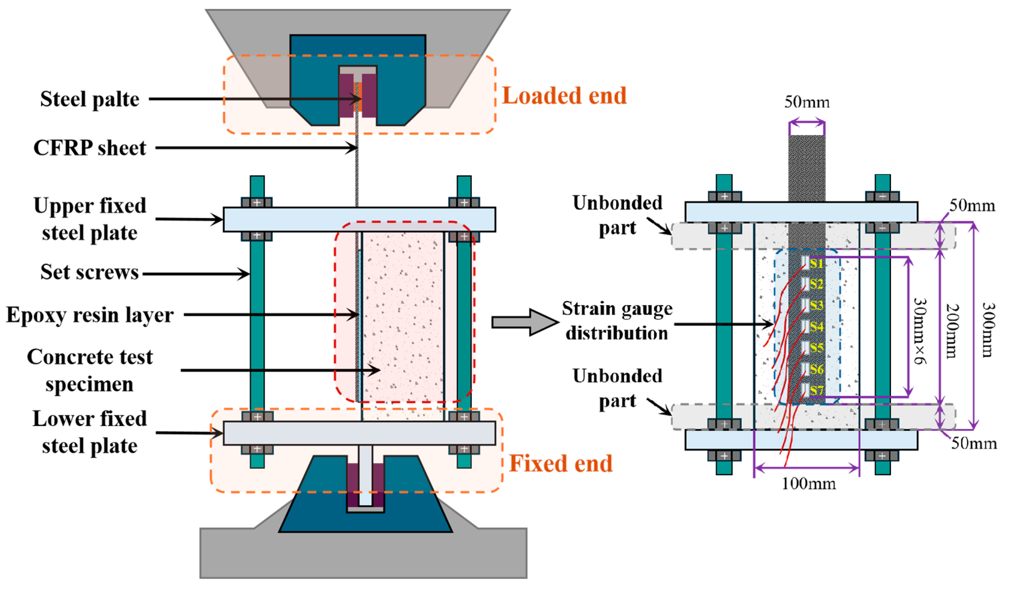
Figure 1 illustrates the customized test apparatus and instrumentation layout used to evaluate the bond performance at the CFRP–concrete interface. The concrete prism specimen was laterally confined by a steel frame and axially anchored to a rigid steel base using high-strength bolts at both the loaded and fixed ends, effectively restraining rotational and translational movement during loading. To prevent premature failure at the gripping zone, a 50 × 50 mm Q235 steel plate was bonded to the CFRP sheet at the loaded end using high-strength epoxy resin for local reinforcement. A universal testing machine applied a monotonic tensile load to the CFRP sheet at a constant displacement rate of 1 mm/min. As shown in the right view of Figure 1, seven strain gauges labeled S1 through S7 were uniformly installed along the bonded length of the CFRP sheet to measure the strain distribution along the FRP–concrete interface. The data were collected in real time using a static strain acquisition system.

3. Effect of Freeze–Thaw Cycles on CFRP-Concrete Bond Behavior

3.1. Failure Modes and Ultimate Bond Strength

The single-lap shear tests revealed consistent failure characteristics across all FT conditions, as illustrated in Figure 2. All specimens primarily failed through interfacial debonding between the CFRP sheet and the concrete substrate, accompanied by partial peeling of the surface concrete layer. No noticeable variations in crack morphology or failure pattern were observed with increasing FT cycles. The cumulative influence of FT exposure was mainly manifested in the gradual degradation of interfacial adhesion and the formation of microcracks within the interfacial transition zone (ITZ), whereas the CFRP sheets and the bulk concrete remained structurally intact.

As illustrated in Figure 3, the ultimate bond strength decreased progressively with the number of FT cycles. Compared with the uncycled control group, reductions of 6.0%, 13.6%, 16.3%, and 18.5% were recorded after 50, 100, 150, and 200 cycles, respectively. The degradation rate was more pronounced within the first 100 cycles and became less significant thereafter, indicating that most interfacial deterioration occurred during the early stage of FT exposure, whereas subsequent cycles primarily propagated existing defects and caused a gradual reduction in the residual bond capacity.

3.2. Strain and Stress Distribution

This study conducted single-lap shear tests on FRP-concrete specimens and collected strain distribution data by attaching strain gauges to the specimen surfaces. During the initial loading phase, the strain values recorded by different gauges showed minimal variation, making it difficult to capture the strain distribution accurately. To address this, the analysis focused only on strain data corresponding to 65–100% of the ultimate load. Additionally, due to the gauge length limitations of the strain gauges and the inherent randomness associated with internal cracking and heterogeneous material composition in concrete, the CFRP strain data were fitted using Equation (1), which is based on the strain distribution model proposed by Dai et al. [28]. This approach helps to eliminate local fluctuations and provides a more accurate representation of the interfacial strain distribution at various load levels.

Table A1. Regression fitting parameters.

Specimen		a	b	c	R2
FT0	0.65 Pu	0.04	6.25	10.34	0.999
	0.70 Pu	0.05	7.23	10.03	0.999
	0.75 Pu	0.06	8.27	10.20	0.999
	0.80 Pu	0.08	9.61	10.14	0.999
	0.85 Pu	0.09	11.22	10.17	0.997
	0.90 Pu	0.13	15.60	10.01	0.978
	0.95 Pu	0.20	24.12	10.00	0.909
	Pu	0.26	33.54	10.00	0.851
FT50	0.65 Pu	0.04	9.76	10.21	0.999
	0.70 Pu	0.08	12.44	10.05	1.000
	0.75 Pu	0.09	13.64	10.01	0.999
	0.80 Pu	0.12	16.82	10.01	0.999
	0.85 Pu	0.14	19.37	10.13	0.994
	0.90 Pu	0.20	27.63	10.00	0.947
	0.95 Pu	0.22	31.63	10.00	0.920
	Pu	0.25	35.36	10.00	0.906
FT100	0.65 Pu	0.02	10.75	10.62	0.993
	0.70 Pu	0.02	9.90	10.16	0.996
	0.75 Pu	0.02	8.38	10.08	0.999
	0.80 Pu	0.07	11.93	10.08	1.000
	0.85 Pu	0.07	11.88	10.08	1.000
	0.90 Pu	0.05	13.96	39.41	1.000
	0.95 Pu	0.09	20.76	37.14	0.999
	Pu	0.13	25.93	32.94	0.993
FT150	0.65 Pu	0.01	14.74	10.47	0.974
	0.70 Pu	0.02	9.38	10.15	0.999
	0.75 Pu	0.04	10.53	10.01	1.000
	0.80 Pu	0.03	12.72	26.09	1.000
	0.85 Pu	0.03	13.55	30.96	1.000
	0.90 Pu	0.01	4.02	127.22	0.834
	0.95 Pu	0.01	5.22	132.97	0.826
	Pu	0.01	6.98	142.98	0.827
FT200	0.65 Pu	0.03	18.05	16.07	0.994
	0.70 Pu	0.01	7.26	43.79	1.000
	0.75 Pu	0.01	8.41	44.71	0.999
	0.80 Pu	0.01	8.10	45.62	1.000
	0.85 Pu	0.02	8.70	45.54	1.000
	0.90 Pu	0.01	9.38	93.28	0.947
	0.95 Pu	0.01	7.61	114.79	0.946
	Pu	0.01	7.23	140.79	0.935

presents the parameter fitting results, while Figure 4 illustrates the fitted strain distribution curves, all of which achieved the coefficient of determination (R²) values exceeding 0.8. The strain distribution displayed a consistent trend: strain increased with load and gradually decreased with distance from the loaded end. As the number of FT cycles increased, the CFRP strain at the ultimate load consistently decreased. Compared with the uncycled specimens, the reductions in strain were 11.0%, 18.8%, 47.8%, and 57.6% after 50, 100, 150, and 200 FT cycles, respectively. These results clearly indicate that FT exposure markedly weakened the interfacial stress-transfer capacity between the FRP and concrete.

$$\epsilon (x)={\displaystyle \frac{a/b}{1+e^{\frac{x-\mathrm{c}}{b}}}},$$

(1)

where ε(x) is the FRP strain at any position x from the loading end, and a, b, and c are the nonlinear regression fitting parameters, respectively.

To minimize local fluctuations and better capture the overall distribution, the measured strain profiles were fitted using the nonlinear regression model proposed by Dai et al [28]. This fitting approach provides a continuous and smooth representation of the strain distribution while preserving the experimental trend. On this basis, the local bond stress at the FRP–concrete interface was calculated according to Equation (2), where the interfacial shear stress is derived from the gradient of the fitted CFRP strain curve and the mechanical properties of the FRP. The results are presented in Figure 5.

The findings clearly demonstrate that FT cycles markedly degraded the interfacial bond performance. Compared with the unconditioned specimens, The peak shear stress (${\tau }_{max}$) decreased by 53–80%, and its peak position progressively shifted away from the loading end as the number of FT cycles increased. This behavior reflects a substantial reduction in local stress-transfer efficiency near the loaded region and a gradual extension of the effective stress-transfer zone toward areas with less deterioration. In addition, although the peak bond stress declined, the corresponding interfacial slip increased, implying that stiffness degradation delayed the mobilization of shear stress along the bonded length.

$$\tau (x)=E_f{t}_f{\displaystyle \frac{d\epsilon (x)}{dx}}=-E_f{t}_f{\displaystyle \frac{a}{b^2}}\left({\displaystyle \frac{e^{\frac{x-c}{b}}}{{\left(1+e^{\frac{x-c}{b}}\right)}^2}}\right),$$

(2)

where $\tau$(x) is the bond stress at any location x from the loading end, t_f is the thickness of the CFRP sheet, and E_f is the modulus of elasticity of the CFRP sheet.

3.3. Bond-Slip Relationship

This study adopted the theoretical framework of the modified Dai model proposed by Zhang et al. and employed the interface mechanics formulation presented in Equation (4) to calculate the slip between CFRP and concrete, as well as to establish the interfacial shear stress–slip relationship [10]. Based on the experimental data and the fitted strain distributions, the bond stress–slip curves at the FRP–concrete interface are illustrated in Figure 6. The results demonstrate that the interfacial behavior exhibits a typical nonlinear response: the shear stress increases rapidly with slip until reaching a peak value, followed by a gradual softening stage, and ultimately leading to complete debonding of the interface [29].

As summarized in

Table 1. Key bond–slip parameters of the FRP–concrete interface under different FT cycles.

Freeze–Thaw Cycles	${\mathit{\tau }}_{\mathit{m}\mathit{a}\mathit{x}}$ (MPa)	Sf (mm)	Su (mm)
0	10.95	0.030	0.29
50	5.13	0.056	0.47
100	4.80	0.047	0.40
150	4.02	0.005	0.04
200	2.13	0.008	0.06

, all key bond–slip parameters exhibited a continuous and progressive decline with increasing FT cycles. The ${\tau }_{max}$ decreased markedly from 10.95 MPa to 2.13 MPa, while both the slip corresponding to ${\tau }_{max}$(S_f) and the ultimate slip (S_u) showed significant reductions at higher cycles, indicating a substantial deterioration in both interfacial strength and deformability. It is noteworthy that ${\tau }_{max}$ decreased sharply within the first 50 FT cycles but declined more slowly during 100–200 cycles. This trend reflects the two-stage evolution of interfacial degradation.

During the initial stage, intensive microcracking rapidly weakened the local stiffness and disrupted the continuity of stress transfer. As degradation progressed, the interface entered a relatively stable phase, in which the weak regions near the loading end had already been damaged, and the subsequent damage rate became considerably lower. Consequently, ${\tau }_{max}$ exhibited only a gradual reduction in the later stage. Furthermore, the slight increase in S_u implies that early microdamage may have facilitated limited stress redistribution, temporarily enhancing local deformability.

To complement the quantitative results, Figure 7 presents representative bond–slip curves reconstructed from the measured parameters under different FT conditions. In the figure, solid lines represent the bond–slip curves calculated from the experimental data, while dashed lines denote the bilinear bond–slip model constructed based on three key experimental points, namely (0, 0), (S_f, ${\tau }_{max}$), and (S_u, 0). As the number of FT cycles increases, the progressive flattening and shortening of the curves clearly illustrate the gradual loss of interfacial ductility and the transition from ductile to brittle behavior.

$$S(x)={\displaystyle {\int }_0^{\infty }\frac{d\epsilon (x)}{dx}dx=a\ln \left(1+e^{-\frac{x-c}{b}}\right)}$$

(3)

$$\tau (S)=E_f{t}_f{\displaystyle \frac{a}{b^2}}{e}^{-{\displaystyle \frac{S}{a}}}(1-e^{-{\displaystyle \frac{S}{a}}})$$

(4)

3.4. Interfacial Fracture Energy

Based on Equation (5), the interfacial fracture energy (G_f) corresponding to the ${\tau }_{max}$ was calculated. The results revealed a pronounced decline in G_f with increasing FT cycles. In the unexposed state (0 FT cycles), the fracture energy was 0.918 N/mm, reflecting a relatively intact interface with robust bonding performance. After 50 and 100 FT cycles, the G_f decreased by 19.3% and 35.2%, respectively, relative to the initial value, reflecting the progressive deterioration of the ITZ and the consequent reduction in bonding efficiency. When the number of FT cycles increased to 150 and 200, G_f dropped by more than 90% compared with its value at 100 cycles, suggesting that the interface had undergone severe structural degradation. The continuous and accelerated reduction in G_f clearly demonstrates the cumulative and irreversible nature of FT-induced damage at the FRP–concrete interface.

$$G_f={\displaystyle {\int }_0^{S_u}\tau (S)}dS$$

(5)

3.5. Mechanistic Interpretation of Freeze–Thaw Damage

FT cycles impose coupled hydraulic and thermal stresses on the FRP–concrete interface. As external moisture penetrates the concrete matrix and ITZ, ice formation during freezing generates internal tensile and hydraulic pressures that exceed the tensile strength of the surrounding cementitious material, initiating microcracks along the epoxy–concrete boundary [9]. The repeated phase transition of water further accelerates the nucleation and propagation of cracks, reducing local stiffness and disrupting stress transfer efficiency [13,30]. Simultaneously, the mismatch in thermal expansion between the epoxy and concrete causes cyclic shear stress accumulation, while moisture-induced embrittlement or plasticization of the epoxy matrix exacerbates interfacial degradation [31,32]. As a result, fracture energy and bond strength decline progressively, and failure modes shift from cohesive concrete delamination to adhesive debonding. With increasing FT cycles, surface crack density and connectivity grow, reducing the effective load-bearing area and causing the stress transfer zone to migrate toward less deteriorated regions [8,10]. These coupled mechanisms collectively weaken both mechanical interlocking and chemical bonding, ultimately resulting in an exponential decline in shear capacity and fracture resistance at the FRP–concrete interface [33].

3.6. Degradation Model of Interfacial Parameters

To quantitatively characterize the degradation of FRP–concrete interfacial performance under FT cycles, exponential regression models were established based on the experimentally obtained bond parameters. The variation in each parameter with the number of FT cycles (N) is expressed by Equation (6), and its logarithmic form yielded a linear relationship, as shown in Equation (7). The decay coefficient k and initial parameter P₀ were determined through least-squares linear regression, while the goodness of fit was evaluated using the R². The fitted results are shown in Figure 8, where colored circular markers represent the experimentally measured parameter values, and solid curves denote the exponential fitting results. Most interfacial parameters exhibit exponential decay with increasing N. Among all parameters, G_f exhibits the highest deterioration rate and P_u the lowest, indicating that freeze–thaw damage predominantly weakens the energy dissipation and deformation capacities of the interface rather than its peak load-bearing ability.

$$P_N=P_0{e}^{-kN}$$

(6)

$$\ln P_N=\ln P_0-kN$$

(7)

where, N is the number of FT cycles, P_N represents the value of an interfacial bond parameter after N FT cycles, P₀ is the initial parameter before FT exposure, and k denotes the exponential decay coefficient.

4. Prediction Based on Machine Learning Models

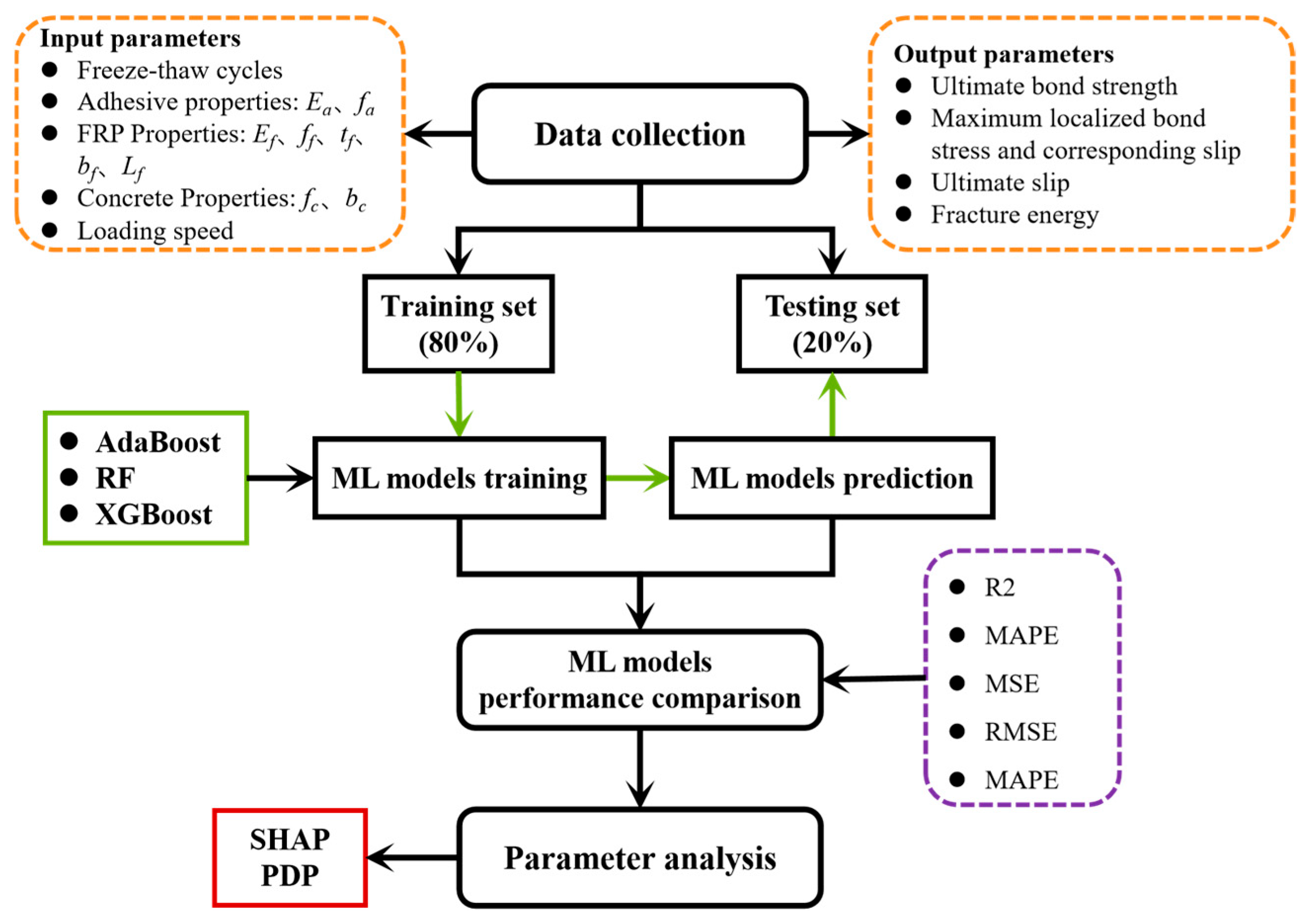
The workflow of the machine learning prediction process is illustrated in Figure 9. First, data on the bond performance of FRP-concrete interfaces were collected from experimental results and relevant literature, followed by data preprocessing. Subsequently, machine learning models were employed to predict key bond performance parameters, and hyperparameters were tuned using optimization algorithms to enhance model performance. The predictive accuracy of different models was then compared using evaluation metrics to identify the optimal model. Finally, SHapley Additive exPlanations (SHAP) analysis was used to quantify the contribution of each input variable to bond performance, and partial dependence plots (PDPs) were employed to reveal the nonlinear influence trends of critical factors.

4.1. Data Collection and Pre-Processing

In this study, considering the limited availability of experimental data on FRP–concrete interfaces under FT conditions, a comprehensive dataset covering both ambient and FT exposure was established by integrating data from existing literature with experimental results obtained in this work. The key input parameters in the dataset included the number of FT Cycles, elastic modulus of the adhesive (E_a), tensile strength of the adhesive (f_a), elastic modulus of the FRP (E_f), tensile strength of the FRP (f_f), FRP thickness (t_f), FRP width (b_f), FRP bond length (L_f), compressive strength of the concrete (f_c), concrete width (b_c), and loading rate (v).

To ensure the integrity of the dataset, the Local Outlier Factor (LOF) method was employed for anomaly detection and data cleaning prior to model development. The LOF algorithm evaluates the local density deviation of each sample relative to its neighbors, effectively identifying points that are isolated in the multidimensional feature space. Samples with abnormally low local densities are considered outliers, as they often represent physically or statistically inconsistent data patterns. The parameters were set to n_neighbors = 20 and contamination = 0.1, following standard practice for medium-sized datasets. The LOF analysis was conducted before the dataset was divided into training and testing subsets. A total of 33 samples exhibiting low local density values were identified and removed, resulting in 299 valid samples for subsequent modeling. Notably, the samples detected as outliers did not show extreme deviations in individual features but rather displayed uncommon feature combinations, leading to sparse distributions in the multidimensional space that could introduce noise to regression training. The corresponding statistical characteristics are summarized in

Table 2. Statistical analysis of input and output parameters.

Parameter		Unit	Min	Max	Mean	SD	COV	Skew
Input	FT Cycles	-	0	300	12.04	33.57	278.79	4.25
	Ea	GPa	0.39	10	3.96	2.24	56.56	1.75
	fa	MPa	11.8	55.5	37.39	12.83	34.31	−0.30
	Ef	GPa	35	304.8	187.60	79.87	42.58	−0.71
	ff	MPa	308.55	4340	2942.14	1309.70	44.52	−0.89
	tf	mm	0.11	3	0.57	0.90	158.85	2.02
	bf	mm	10	100	47.37	17.70	37.36	1.36
	Lf	mm	50	330	217.18	62.22	28.65	−0.01
	fc	MPa	17.9	75.5	35.48	9.74	27.47	0.87
	bc	mm	75	400	140.72	74.74	53.12	2.68
	v	mm/min	0.005	90	6.94	18.23	262.84	3.43
Output	Pu	kN	2.39	60.9	13.90	8.55	61.53	2.47
	${\tau }_{max}$	MPa	0.241	15.71	5.40	2.82	52.32	1.13
	Sf	mm	0.002	0.46	0.06	0.06	96.79	2.80
	Su	mm	0.004	2.37	0.56	0.44	77.82	1.30
	Gf	N/mm	0.002	3.53	1.06	0.75	70.61	1.25

Note: P_u is the ultimate bond strength, ${\tau }_{max}$ is the local maximum bond stress, S_f is the slip corresponding to ${\tau }_{max}$, S_u is the ultimate slip, G_f is the interfacial fracture energy.

. Detailed information on the dataset is provided in the Supplementary Materials.

Moreover, to investigate the interrelationships among the variables in the dataset, Figure 10 displays the Pearson correlation coefficient matrix between the input and output parameters. A higher absolute value of the coefficient indicates a stronger correlation between two variables. It was observed that, except for the correlation between t_f and E_a, which exceeded 0.8 in absolute value, the correlation coefficients among the remaining parameters were all below 0.8, suggesting relatively low interdependencies.

4.2. Machine Learning Models

4.2.1. Adaptive Boosting (AdaBoost)

The AdaBoost model is an ensemble learning method that iteratively trains a series of weak classifiers, adjusting the weights of samples in each iteration to increase the model’s focus on misclassified instances [34]. Ultimately, the predictions of all weak classifiers are combined through a weighted majority vote to form a strong classifier.

4.2.2. Random Forest (RF)

Random Forest (RF) is an ensemble learning technique that constructs multiple decision trees by training on different subsets of the original dataset generated through bootstrap sampling with replacement [35]. For regression tasks, the RF model produces its final output by averaging the predictions from all individual decision trees.

4.2.3. Extreme Gradient Boosting (XGBoost)

XGBoost is an efficient gradient boosting framework based on the Gradient Boosted Decision Tree (GBDT) technique. It improves model performance by iteratively constructing tree models to minimize prediction residuals [36].

4.3. ML Model Development

4.3.1. Performance Evaluation Indicators

To ensure a comprehensive and rigorous assessment of the predictive performance of different machine learning models, five evaluation metrics were adopted in this study: Mean Absolute Error (MAE), Mean Absolute Percentage Error (MAPE), Mean Squared Error (MSE), Root Mean Squared Error (RMSE), and the coefficient of determination (R²). The corresponding mathematical formulations are provided in

Table 3. Evaluation indicators and equations.

Evaluation Indicators	Equation
MAE	$MAE={\displaystyle \frac{1}{n}}{\displaystyle \sum _{i=1}^n\left|y_i-{\widehat{y}}_i\right|}$
MAPE	$MAPE={\displaystyle \frac{1}{n}}{\displaystyle \sum _{i=1}^n\left|\frac{y_i-{\widehat{y}}_i}{y_i}\right|}\times 100\%$
MSE	$MSE={\displaystyle \frac{1}{n}}{\displaystyle \sum _{i=1}^n{(y_i-{\widehat{y}}_i)}^2}$
RMSE	$RMSE=\sqrt{MSE}$
R2	$R^2=1-{\displaystyle \frac{{\displaystyle \sum _{i=1}^n{(y_i-{\widehat{y}}_i)}^2}}{{\displaystyle \sum _{i=1}^n{(y_i-\overline{y})}^2}}}$

Note: n denotes the total number of samples; $y_i$ and ${\widehat{y}}_i$ represent the actual and predicted values, respectively; $\overline{y}$ denotes the mean of the actual values.

. These metrics collectively assess the accuracy, magnitude of prediction errors, and the degree of data fitting. The use of these multidimensional evaluation criteria provides robust data support for model selection and optimization.

4.3.2. Model Training and Optimization

To accurately capture the distinct degradation patterns of different interfacial properties, a multi-task prediction framework was established, in which five independent sub-models were constructed to predict the key bond–slip parameters P_u, ${\tau }_{max}$, S_f, S_u, and G_f, respectively. Although these parameters are interrelated in the physical sense, their statistical distributions, magnitudes, and sensitivities to FT damage differ considerably. Therefore, training independent sub-models under a unified framework enables each model to specialize in learning its characteristic mapping relationship while maintaining consistency in data processing and evaluation.

The Optuna hyperparameter optimization framework was applied separately to each sub-model to determine the optimal parameter configuration. Optuna integrates Bayesian optimization with the Tree-structured Parzen Estimator (TPE) algorithm, allowing adaptive and efficient exploration of the hyperparameter search space to enhance predictive performance [37]. To ensure comparability, all sub-models shared identical input features, optimization criteria, and search ranges, with 300 Optuna trials conducted for each model. The optimal configuration was selected based on the minimum mean squared error (MSE) obtained on the validation set.

Table 4. Hyperparameter optimization settings.

ML Model	Hyperparameters	Tuned Range	Optimal Hyperparameter
			Pu	${\mathit{\tau }}_{\mathit{m}\mathit{a}\mathit{x}}$	Sf	Su	Gf
AdaBoost	n_estimators	[50, 1000]	156	78	637	95	554
	learning_rate	[0.001, 0.3]	0.002	0.038	0.189	0.109	0.001
	max_depth	[2, 20]	9	10	7	10	9
RF	n_estimators	[50, 1000]	85	205	487	416	325
	max_depth	[2, 20]	10	10	8	10	9
XGBoost	n_estimators	[50, 1000]	372	234	402	136	113
	learning_rate	[0.001, 0.3]	0.279	0.023	0.148	0.205	0.088
	max_depth	[2, 20]	55	7	4	3	4

lists the unified hyperparameter search ranges and the optimal configurations determined for each sub-model under the Optuna optimization framework.

To evaluate the convergence behavior and generalization capability of the optimized models, learning curves were plotted based on the R² with increasing training sample proportions, as shown in Figure 11. The solid lines with colored circular and triangular markers illustrate the evolution of training and test set results for different ML models, respectively. For all prediction tasks, the training R² values remained consistently high (>0.95), while the validation R² values exhibited a monotonic increase and gradually converged. When the training size was below 60 samples, large fluctuations and even negative validation R² values were observed, especially for S_f and S_u. As the training data increased, the validation R² of all models progressively improved and stabilized within the range of 0.75–0.90, demonstrating that the models effectively captured the underlying feature–response relationships once sufficient data coverage was achieved. Among the three algorithms, XGBoost consistently exhibited the highest and smoothest convergence trend, with the smallest generalization gap between the training and validation curves, indicating its superior robustness and generalization performance.

In addition, to further verify the robustness and statistical consistency of the developed models, supplementary experiments were conducted under five different random seeds (0, 7, 42, 99, and 123). For each of the five output parameters, the mean and standard deviation of the R² and RMSE were calculated, and paired t-tests were performed based on R² to evaluate the statistical significance of inter-model differences. As shown in

Table A2. Statistical and performance evaluation of ML models.

Output	Model	Mean R2	Std. of R2	Mean RMSE	Std. of RMSE	t	p
Pu	XGBoost	0.906	0.012	2.590	0.477	-	-
	RF	0.892	0.025	2.773	0.636	1.853	0.137
	AdaBoost	0.879	0.012	2.913	0.381	3.521	0.024
${\tau }_{max}$	XGBoost	0.867	0.030	0.925	0.146	-	-
	RF	0.828	0.045	1.040	0.115	1.621	0.180
	AdaBoost	0.858	0.064	0.941	0.236	0.490	0.650
Sf	XGBoost	0.763	0.191	0.026	0.013	-	-
	RF	0.776	0.161	0.025	0.011	−0.655	0.548
	AdaBoost	0.626	0.208	0.033	0.012	1.769	0.152
Su	XGBoost	0.950	0.013	0.093	0.011	-	-
	RF	0.927	0.024	0.111	0.014	1.737	0.157
	AdaBoost	0.940	0.047	0.095	0.027	0.572	0.598
Gf	XGBoost	0.935	0.014	0.174	0.016	-	-
	RF	0.892	0.044	0.219	0.036	2.095	0.104
	AdaBoost	0.916	0.030	0.195	0.038	1.365	0.244

, the XGBoost model consistently achieved high predictive accuracy across all outputs, with mean R² values ranging from 0.76 to 0.95 and relatively low RMSE and variance, indicating low sensitivity to random initialization and strong stability. In comparison, RF achieved comparable accuracy but with higher variability, whereas AdaBoost showed lower accuracy in P_u and S_f, indicating weaker adaptability. Although the paired t-tests indicated that the inter-model differences were not statistically significant in most prediction tasks (p > 0.05), XGBoost achieved the highest mean R² and lowest RMSE in four out of five outputs.

Overall, these results confirm that the optimized XGBoost model possesses superior stability and generalization capability across multiple prediction tasks.

4.4. ML Model Prediction Performance

This study analyzed the performance of three ML models in predicting the bond behavior at the FRP–concrete interface using multiple evaluation metrics. The models were compared based on their performance across five key output parameters. Detailed results of the evaluation metrics are presented in

Table A3. Evaluation metrics of ML models for predicting interface performance parameters.

Output	Statistics	AdaBoost			RF			XGBoost
		Train	Test	Total	Train	Test	Total	Train	Test	Total
Pu	MSE	12.034	13.319	12.292	10.21	6.924	9.551	3.346	6.498	3.978
	RMSE	3.469	3.65	3.506	3.195	2.631	3.09	1.829	2.549	1.995
	MAE	2.585	2.747	2.618	1.805	1.756	1.795	0.742	1.46	0.887
	MAPE	25.152	30.569	26.239	14.585	19.738	15.619	4.603	11.606	6.008
	R2	0.832	0.830	0.831	0.857	0.912	0.869	0.953	0.917	0.945
${\tau }_{max}$	MSE	1.97	2.283	2.032	0.316	0.699	0.393	0.246	0.574	0.312
	RMSE	1.403	1.511	1.426	0.562	0.836	0.627	0.496	0.757	0.558
	MAE	1.1	1.192	1.119	0.404	0.626	0.449	0.343	0.587	0.392
	MAPE	29.276	41.047	31.638	10.212	20.03	12.182	8.728	17.355	10.459
	R2	0.764	0.593	0.744	0.962	0.875	0.951	0.971	0.898	0.961
Sf	MSE	0.001	0.001	0.001	0.001	0	0.001	0.001	0	0.001
	RMSE	0.031	0.037	0.033	0.026	0.018	0.024	0.025	0.016	0.023
	MAE	0.015	0.021	0.016	0.01	0.01	0.01	0.009	0.011	0.009
	MAPE	44.565	47.208	45.096	24.187	24.469	24.243	24.428	22.842	24.110
	R2	0.765	0.337	0.718	0.841	0.849	0.841	0.852	0.882	0.856
Su	MSE	0.026	0.032	0.027	0.006	0.009	0.006	0.004	0.008	0.005
	RMSE	0.161	0.179	0.165	0.075	0.097	0.08	0.064	0.091	0.07
	MAE	0.12	0.128	0.122	0.048	0.065	0.052	0.042	0.063	0.046
	MAPE	67.689	67.629	67.677	14.285	19.77	15.386	13.448	20.655	14.894
	R2	0.859	0.856	0.859	0.970	0.958	0.967	0.978	0.963	0.974
Gf	MSE	0.125	0.122	0.124	0.015	0.031	0.018	0.022	0.026	0.023
	RMSE	0.353	0.349	0.353	0.122	0.176	0.135	0.147	0.160	0.150
	MAE	0.239	0.271	0.246	0.088	0.133	0.097	0.108	0.121	0.110
	MAPE	79.158	101.221	83.585	21.067	34.706	23.804	36.313	37.208	36.493
	R2	0.791	0.693	0.778	0.975	0.922	0.968	0.964	0.935	0.960

, covering the training set, testing set, and the entire dataset.

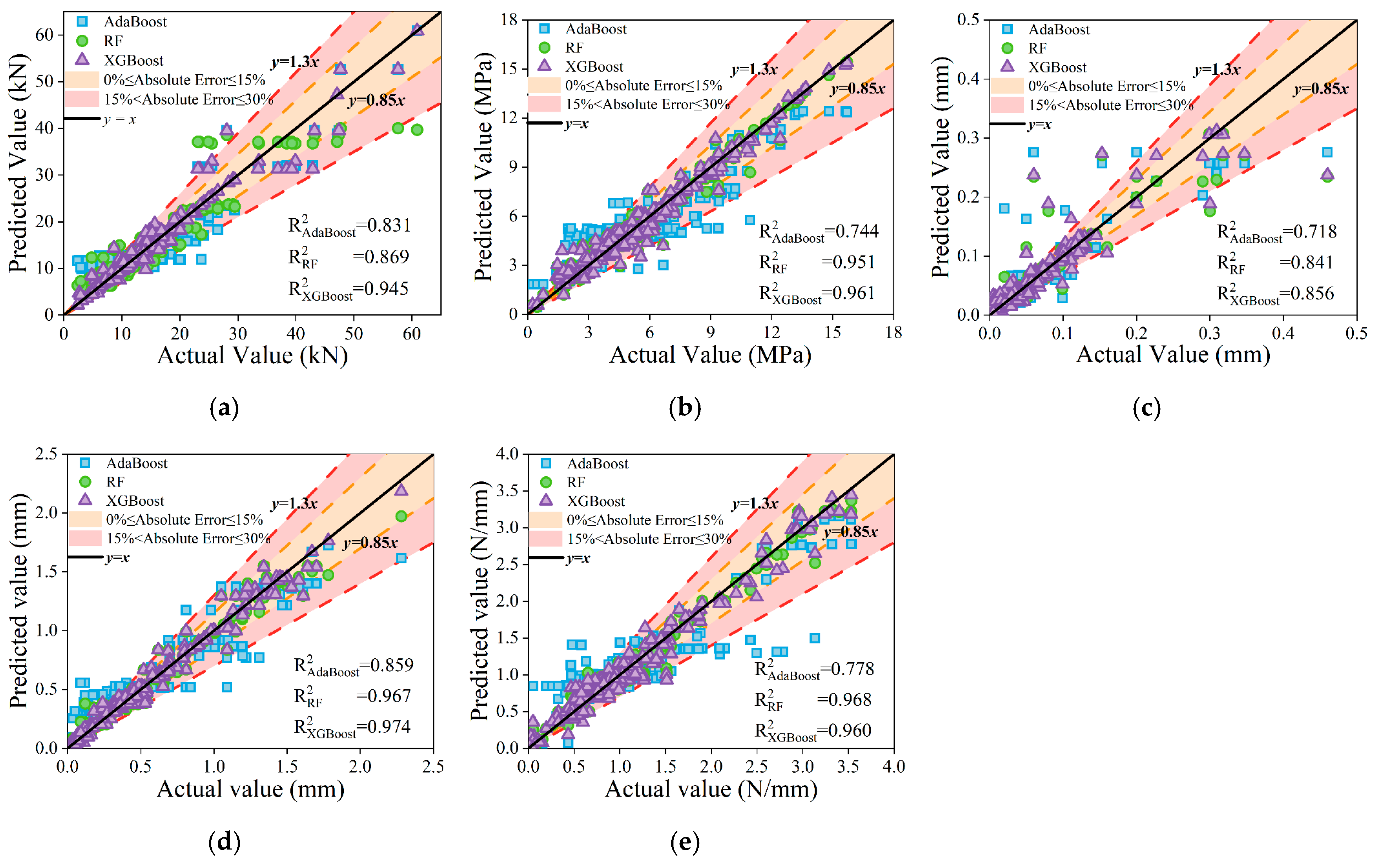
As illustrated in Figure 12, notable differences were observed in the fitting performance between predicted and actual values across the entire dataset for the three ML models. Among them, the XGBoost model demonstrated particularly outstanding performance, especially in predicting the parameters P_u, ${\tau }_{max}$, S_f, and S_u, with corresponding R² values of 0.945, 0.961, 0.856, and 0.974, each exceeding those of the AdaBoost and RF models by more than 9%. In addition, for these four parameters, the RMSE values obtained by the XGBoost model were 1.995 kN, 0.558 MPa, 0.023 mm, and 0.070 mm, respectively, while the MAPE values were 6.01%, 10.46%, 24.11%, and 14.89%. These results further demonstrate the strong predictive capability of the XGBoost model for key indicators of FRP–concrete bond behavior. In comparison, although the overall predictive accuracy of the RF model was slightly inferior to that of XGBoost, it exhibited superior performance in predicting the G_f, achieving an R² value of 0.967, which was higher than XGBoost’s 0.960. This slight advantage suggests that the RF model may be better suited for capturing the characteristics associated with interfacial fracture energy. Among all the models, AdaBoost demonstrated the weakest performance, with R² values consistently lower than those of both XGBoost and RF across all prediction tasks. This indicates that AdaBoost struggles to accurately model the complex nonlinear behavior of the FRP–concrete interface.

Overall, the XGBoost model demonstrated outstanding fitting accuracy and generalization ability across all prediction tasks. It consistently exhibited lower prediction errors on the training set, testing set, and the entire dataset. Therefore, XGBoost can be considered the most effective machine learning model for predicting the bond performance at the FRP–concrete interface.

4.5. Analysis of Input Features

4.5.1. SHAP Analysis

In this study, the XGBoost machine learning model was employed in conjunction with the SHAP (Shapley Additive Explanations) analysis method to investigate the influencing factors governing the bond performance at the FRP–concrete interface. The SHAP approach enables a quantitative assessment of the contribution of each input variable to the model’s predictions, thereby revealing the key factors affecting the interfacial behavior between FRP sheets and concrete.

Table 5. Feature importance ranking for different outputs.

Feature Name	Pu		${\mathit{\tau }}_{\mathit{m}\mathit{a}\mathit{x}}$		Sf		Su		Gf
	Percentage	Rank	Percentage	Rank	Percentage	Rank	Percentage	Rank	Percentage	Rank
FT Cycles	3.4	9	7.3	6	0.8	10	3.4	10	3.8	9
Ea	7.3	6	5.6	7	3.6	7	5.4	7	10.7	4
fa	5.9	7	9.9	5	10.3	4	12.1	4	13.7	3
Ef	9.9	5	15.7	2	17.1	3	31.7	1	6.8	7
ff	1.7	10	1.5	11	5.9	5	3.4	9	1.1	10
tf	13.1	3	12.4	4	25.1	2	14.7	2	10.4	5
bf	25.1	1	4.8	8	3.2	8	0.4	11	0.8	11
Lf	3.9	8	3.1	10	26.5	1	5.7	6	6.3	8
fc	12.0	4	20.2	1	3.7	6	6.1	5	14.1	2
bc	0.9	11	3.9	9	0.6	11	13.2	3	8.5	6
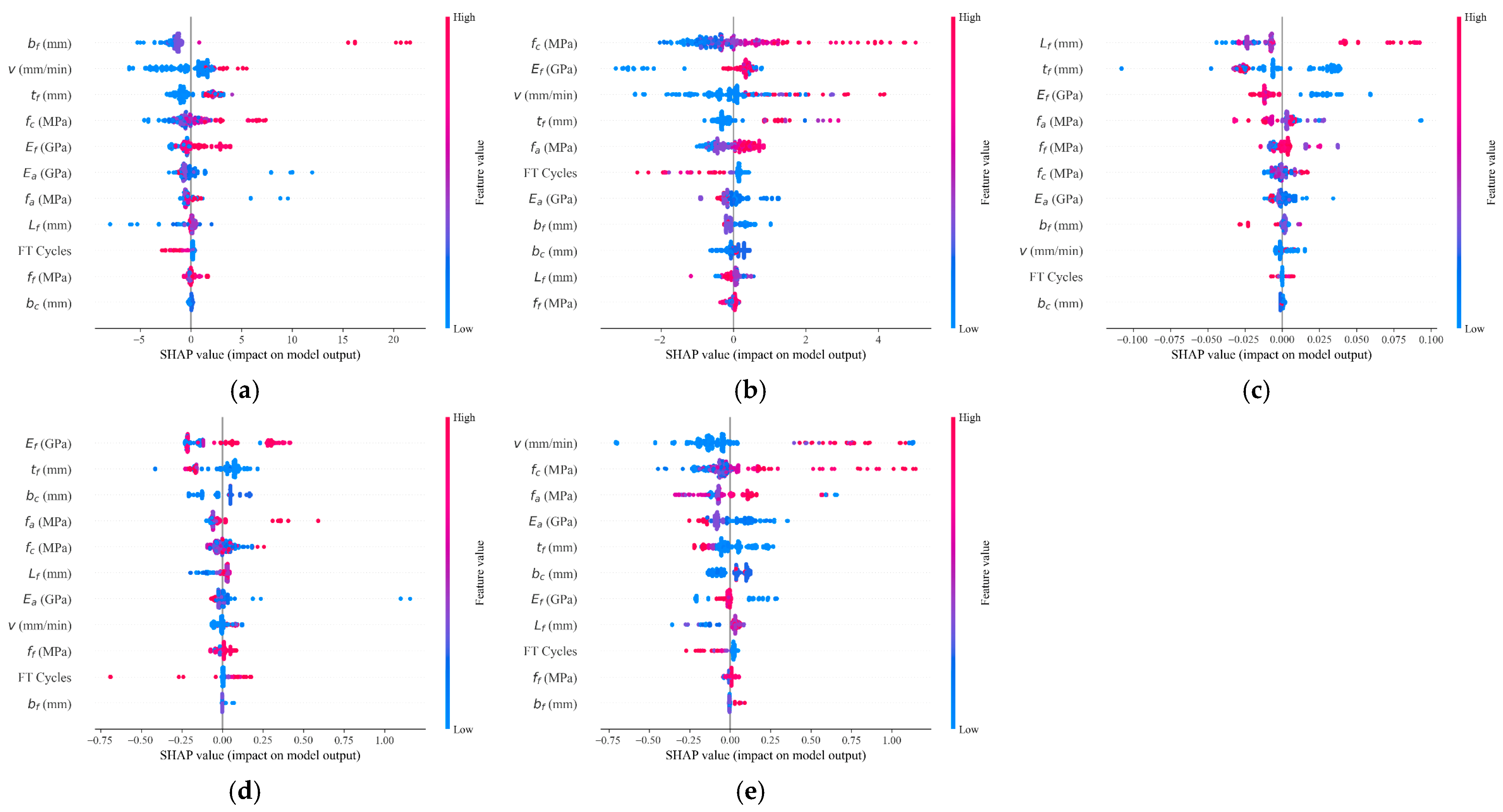
v	16.8	2	15.5	3	3.1	9	3.9	8	24.0	1

summarizes the overall SHAP-based feature importance rankings, highlighting the varying contributions of input variables across different output parameters. Figure 13 further visualizes the distribution of local SHAP values, providing insights into the individual influence of each feature on the model predictions.

In the prediction of the P_u, the b_f was identified as the most influential factor, accounting for 25.1% of the total feature importance. As shown in Figure 13a, an increase in the b_f significantly enhanced the load-bearing capacity of the bond interface. Additionally, the v and t_f contributed 16.8% and 13.1% to the model’s predictions. A higher v was found to accelerate the attainment of P_u, while an increase in t_f contributed to an overall improvement in the structural integrity of the interface.

For the ${\tau }_{max}$, the f_c had the most significant influence, with a feature importance of 20.2%, indicating that high-strength concrete plays a critical role in enhancing ${\tau }_{max}$. The E_f and the v contributed 15.7% and 15.5%, respectively, highlighting the notable impact of both material properties and loading conditions on shear performance.

The slip behavior at the FRP–concrete interface was primarily governed by the mechanical properties and geometric dimensions of the FRP material. In the prediction of the slip corresponding to the S_f, the L_f and t_f were identified as the key influencing factors, with feature importance values of 26.5% and 25.1%, respectively. For the S_u, the most significant factor was the E_f, with a feature importance of 31.7%, followed by the t_f at 14,7%. Materials with higher elastic modulus can effectively improve the interfacial bond stiffness by enhancing constraint at the interface.

In the prediction of G_f, the v was the dominant factor, with a feature importance of 24.0%. An increase in v tends to intensify brittle failure at the bond interface, thereby reducing the G_f. In addition, the fc and f_a had feature importance values of 14.1% and 13.7%, respectively. These material parameters play a critical role in enhancing the energy accumulation and load-bearing capacity of the bonded interface.

Although experimental results indicated that FT cycles had a significant impact on the ${\tau }_{max}$ and S_u, their feature importance in the XGBoost model was relatively low. This is primarily due to the high degree of coupling between the effects of FT cycles and other variables, such as concrete compressive strength and the elastic modulus of the FRP, rather than FT cycles acting as an independent determining factor. While FT degradation does contribute to the deterioration of bond performance, within the analyzed dataset, the influence of material properties—particularly concrete strength and FRP stiffness—was more prominent, thereby reducing the apparent direct contribution of FT cycles in the model.

4.5.2. PDP Analysis

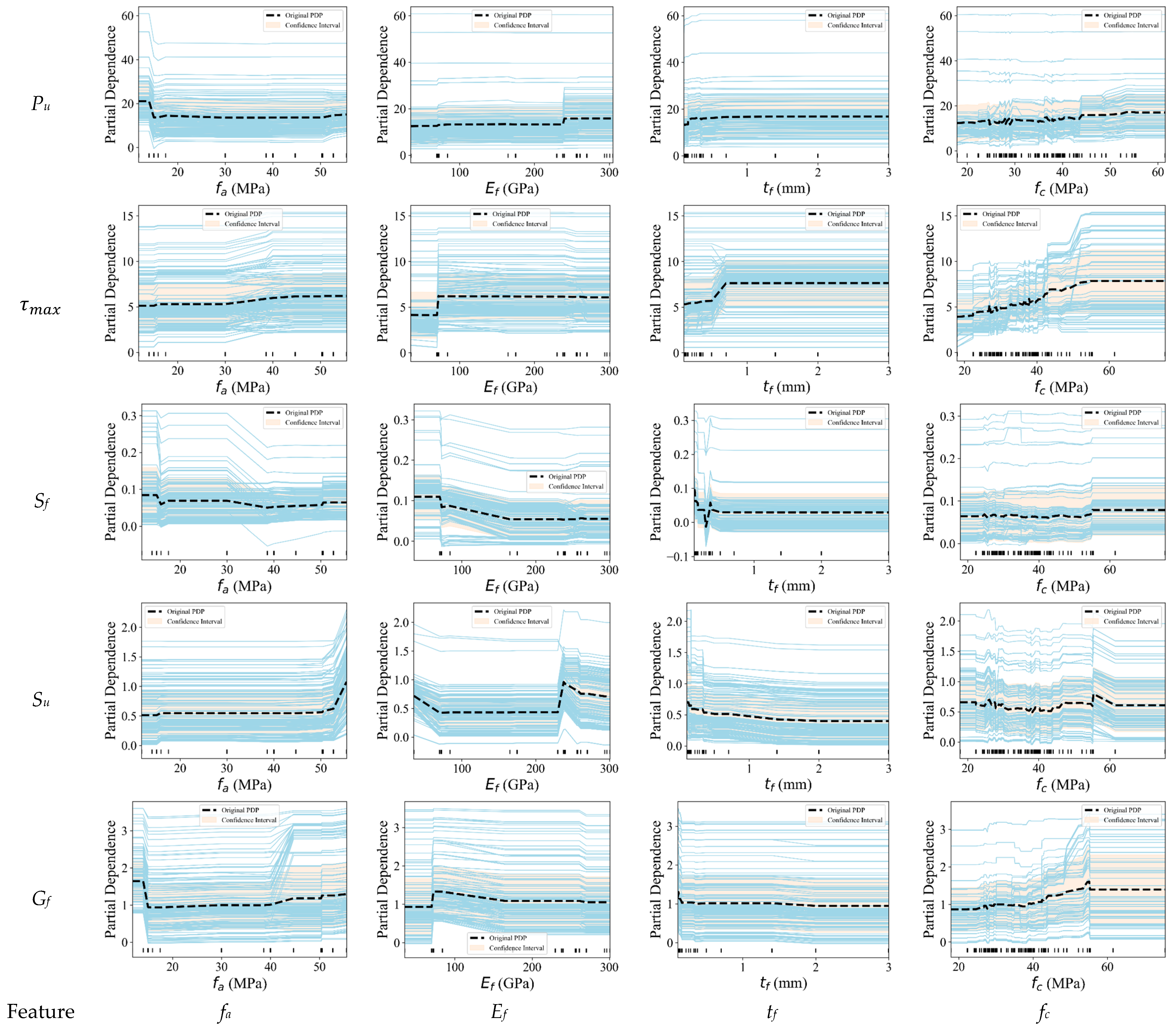
In this study, the application of the SHAP method revealed that the tensile strength of the adhesive layer (f_a), elastic modulus of the FRP (E_f), fiber thickness (t_f), and concrete compressive strength (f_c) exert significant influence on the bond performance at the FRP–concrete interface. These parameters not only demonstrated high feature importance across multiple output variables, but also played a central role in interfacial stress transfer, deformation behavior, and failure modes. However, while SHAP analysis effectively identified the importance and directionality of these features, it did not provide detailed insights into the specific trends of their influence on model outputs or the optimal value ranges. To address this limitation, Partial Dependence Plots (PDPs) were further employed to investigate the influence patterns of these key variables on the predicted outcomes. As shown in Figure 14, the blue PDP curves illustrate the average effect of each feature on the model output. The black vertical lines at the bottom indicate the distribution of sample points across the feature range, and the black dashed line represents the smoothed trend fitted from the PDP, revealing the nonlinear relationship between the feature and the predicted response.

A detailed analysis of Figure 14 identified the optimal range for the f_a to be 15–25 MPa. Within this range, f_a not only enhances the interfacial resistance to debonding, but also avoids the reduction in energy dissipation capacity and the risk of brittle failure caused by excessive adhesive stiffness. For the E_f and t_f of the FRP, the recommended optimal ranges are 70–140 GPa and 1.1–2.0 mm, respectively. Parameters within these intervals contribute to improved stress transfer efficiency and interfacial load-bearing capacity, while reducing premature debonding due to stress concentration. The optimal range for f_c was found to be 30–50 MPa. This range not only enhances the load-bearing capacity of the concrete substrate, but also improves interfacial performance under large slip conditions, enabling greater energy accumulation under high-stress environments. By precisely adjusting these key parameters, the bond performance at the FRP–concrete interface can be significantly improved, thereby optimizing both the overall structural performance and long-term durability.

5. Conclusions

This study integrates experimental testing with interpretable machine learning (ML) to investigate the freeze–thaw (FT)-induced degradation of FRP–concrete interfaces and to establish a quantitative prediction framework for key bond–slip parameters. The main conclusions drawn from this study are as follows:

(1)

The experimental results revealed a consistent failure pattern dominated by interfacial debonding accompanied by surface concrete peeling. The ultimate bond strength decreased by 6.0–18.5%, with the most severe deterioration occurring during the early FT cycles, indicating that the epoxy–concrete interface is the primary weak zone controlling the overall bond performance.

(2)

Freeze–thaw cycling significantly reduced the ductility and energy dissipation capacity of the interface. The maximum strain and peak bond stress decreased by 57.6% and 53–80%, respectively, while the ultimate slip and fracture energy continuously declined. After 200 cycles, fracture energy dropped by more than 90%, suggesting a transition from ductile adhesion to brittle debonding and a near-collapse of the interfacial bond mechanism.

(3)

The XGBoost model demonstrated superior predictive accuracy and generalization among all evaluated algorithms, with R² values of 0.945 for P_u, 0.961 for ${\tau }_{max}$, 0.856 for S_f, 0.974 for S_u, and 0.960 for G_f, accompanied by consistently low RMSE values. It also exhibited stable convergence and low variance under multiple random seeds, confirming its robustness and reliability.

(4)

SHAP and PDP analyses identified adhesive tensile strength, fiber modulus, FRP thickness, and concrete strength as dominant influencing factors. Their effective ranges—15–25 MPa, 70–140 GPa, 1.1–2.0 mm, and 30–50 MPa—define the optimal parameter window for durable bonding performance.

The proposed interpretable machine learning framework provides a quantitative approach for predicting the degradation of FRP–concrete bond performance under freeze–thaw conditions. The identified key parameters and their rational ranges can assist in durability-oriented interface design, while the data-driven framework can be integrated with empirical bond–slip models to support durability evaluation and parameter adjustment under different environmental exposures.