VMD-SSA-LSTM-Based Cooling, Heating Load Forecasting, and Day-Ahead Coordinated Optimization for Park-Level Integrated Energy Systems

Abstract

Park-level integrated energy systems (IESs) are increasingly challenged by rapid electrification and higher penetration of renewable energy, which exacerbate source–load imbalances and scheduling uncertainty. This study proposes a unified framework that couples high-accuracy cooling and heating load forecasting with day-ahead coordinated optimization for an office park in Tianjin. The forecasting module employs correlation-based feature selection and variational mode decomposition (VMD) to capture multi-scale dynamics, and a sparrow search algorithm (SSA)-driven long short-term memory network (LSTM), with hyperparameters globally tuned by root mean square error to improve generalization and robustness. The scheduling module performs day-ahead optimization across source, grid, load, and storage to minimize either (i) the standard deviation (SD) of purchased power to reduce grid impact, or (ii) the total operating cost (OC) to achieve economic performance. On the case dataset, the proposed method achieves mean absolute percentage errors (MAPEs) of 8.32% for cooling and 5.80% for heating, outperforming several baselines and validating the benefits of multi-scale decomposition combined with intelligent hyperparameter searching. Embedding forecasts into day-ahead scheduling substantially reduces external purchases: on representative days, forecast-driven optimization lowers the SD of purchased electricity from 29.6% to 88.1% across heating and cooling seasons; seasonally, OCs decrease from 6.4% to 15.1% in heating and 3.8% to 11.6% in cooling. Overall, the framework enhances grid friendliness, peak–valley coordination, and the stability, flexibility, and low-carbon economics of park-level IESs.

1. Introduction

With accelerating global urbanization, energy demand across industry, transport, buildings, and residential sectors continues to rise, bringing energy consumption issues to the fore. According to the International Energy Agency, the building sector accounts for roughly 30% of global final energy use. Driven by the rapid electrification of end uses such as heating and cooling, electricity demand in buildings is expected to increase by about 35% from 2020 to 2050, and electricity is likely to become the dominant energy carrier in this sector, reaching around two-thirds of total energy consumption [1]. However, a primary energy mix dominated by oil, natural gas, and coal entails environmental pollution and greenhouse gas emissions, exacerbating climate change and ecological stress. Under the dual pressures of resource constraints and environmental requirements, the energy system is accelerating its transition toward clean, low-carbon, and renewable pathways [2].

As a key component of the modern energy internet, the IESs coordinate multiple energy carriers through multi-energy coupling and intelligent scheduling, enabling efficient allocation across energy forms and time scales with notable environmental and economic benefits. In load-intensive scenarios such as parks and industrial parks, IES not only improves on-site energy efficiency but also enhances bulk-grid stability via bidirectional interaction with the power system [3]. Compared with traditionally siloed electricity–heat–gas systems, IESs better meets diversified energy demands and increase renewable-energy accommodation. IES technologies have received wide attention and policy support in more than 80 countries, including the United States [4], Canada [5,6], the European Union [7,8,9], and Japan [10]. Since 2015, China has accelerated research and demonstrations, advancing smart-energy platforms and multi-energy complementarity in various parks under the dual-carbon targets [11]. Nevertheless, park-level IESs still face strong multi-energy coupling, multi-objective trade-offs, and scenario heterogeneity, for which existing models struggle to deliver fine-grained performance.

With high penetration of renewable energy sources such as wind and photovoltaics (PV), both load and generation exhibit stronger uncertainty and volatility, further complicating supply–demand matching and optimal scheduling. To address uncertainty, distributed robust co-scheduling has been proposed to enhance the coordination of multi-region IESs under wind and load uncertainties [12]. On the demand-response (DR) side, multi-timescale, response-aware game-theoretic scheduling has been developed to improve responsiveness to load fluctuations [13]. From the perspectives of user autonomy and multi-energy synergy, multilevel distributed DR and integrated benefit-optimization models have been reported, providing theoretical support for efficient scheduling under complex loads [14,15]. However, under high renewable penetration, relying solely on scheduling and DR is insufficient for real-time balancing. High-accuracy forecasting of diversified loads—particularly cooling and heating—becomes pivotal to improving dispatch precision and flexibility. Load forecasting not only helps depict intrinsic multi-energy couplings but also provides data foundations for system optimization and coordinated multi-energy scheduling, thereby improving energy efficiency and alleviating local supply–demand tensions [16].

In recent years, swarm-intelligence algorithms—such as particle swarm optimization (PSO) [17], the whale optimization algorithm (WOA) [18], the SSA [19], and dung beetle optimization (DBO) [20]—have been widely employed to improve load-forecasting accuracy, often integrated with LSTMs with attention mechanisms and support vector regression (SVR), demonstrating strong modeling and generalization capabilities [21]. To overcome heuristic algorithms’ tendencies to become trapped in local optima and converge slowly, strategies such as chaotic mechanisms, elitist opposition-based learning, and reverse learning have been introduced, significantly enhancing global search capabilities [20]. Consequently, high-performance load forecasting has become a core enabler for addressing IES scheduling challenges and ensuring secure, economic operation.

Meanwhile, deep interaction between IESs and the power grid has become an important direction in modern energy-system evolution. Through buy–sell electricity mechanisms, IESs can realize bidirectional energy flows and flexible load adjustments, while providing ancillary services such as peak shaving and valley filling for the grid [22]. As a key grid-side instrument, DR guides users to adjust consumption during peak or stress periods, increasing flexibility and responsiveness, facilitating renewable integration, and easing grid stress [23]. Park-level IESs, via coordinated scheduling, can achieve higher-level load-side management across electricity–heat–cooling–gas dimensions, advancing the energy internet and jointly improving system reliability and economic performance.

Conventional buy–sell strategies primarily rely on day-ahead scheduling (DAS), typically minimizing procurement costs [24] and maximizing economic benefits [12,13,14,25] based on load and price forecasts. With the deepening application of DR, loads can be flexibly adjusted following grid signals, markedly enhancing adaptability to renewable variability. Integrated DR models covering cooling, heating, electricity, and natural gas have been shown to improve system flexibility and energy efficiency [15]. Studies indicate that transferable loads under DR help shave peaks, fill valleys, and reduce operating costs [26]. However, for large energy consumers such as parks, single-mode DR alone can hardly unlock the full flexibility potential. Leveraging multi-energy coupling to establish deep, coordinated interactions with the grid has become essential to ensure reliability, economic efficiency, and sustainability. Accordingly, diverse objectives—e.g., improving grid responsiveness [27], smoothing load fluctuations [28], and reducing peak–valley gaps [29]—have been formulated to guide the coordinated optimization of IESs and achieve efficient grid interactions, thereby laying a theoretical foundation for enhancing park energy efficiency and supporting low-carbon transitions.

Under the current research context, the literature addressing multi-energy carriers, park-scale load forecasting, and energy-system optimization has grown progressively. However, existing work often focuses on single-energy coupling (e.g., electricity–heat or electricity–gas) or on limited park settings, and lacks systematic, cross-type comparisons of forecasting accuracy, scheduling performance, and economic outcomes across diverse park types [12,13,14,15,21,22,23,24,25,26,27,28,29,30]. Although recent reviews have cataloged forecasting techniques from traditional time series to deep learning and have surveyed multi-time-scale optimization and multi-energy coordination approaches (including day-ahead and real-time horizons), there remains a gap in directly benchmarking these methods within a unified park-level IES framework to enable meaningful cross-study comparisons [12,13,14,15,23,24,25,26,27,28]. Addressing this benchmarking gap is critical, as the literature increasingly recognizes that robust park-level coordination requires not only accurate predictions but also end-to-end optimization that accounts for the interdependencies and couplings among electricity, heating, cooling, and storage, thereby delivering more comprehensive economic and environmental benefits [12,13,14,15,21,22,23,24,25,26,27,28,29,30,31].

Overall, under ongoing energy transition and dual-carbon targets, park-level IESs play an increasingly vital role in multi-energy complementarity, energy-efficiency improvement, and clean, low-carbon development. Yet, strong volatility and high uncertainty on the load side challenge traditional historical data-based operation methods, which fall short of fine-grained, smart operation and management needs. The accuracy of load forecasting directly influences the economic efficiency and security of dispatch. Thus, a central research challenge is the deep integration of high-accuracy load forecasting with coordinated multi-energy optimization to enable efficient source–load integrated scheduling for park-level IESs, coupled with robust evaluation frameworks that can compare forecasting accuracy, scheduling outcomes, and economic performance across diverse park contexts.

The main contributions are as follows:

• A cooling–heating load-forecasting model is proposed that integrates Pearson correlation analysis, VMD, and SSA-LSTM. Correlation-based feature screening, signal decomposition for nonstationary, multi-scale characteristics, and swarm-intelligence-based hyperparameter tuning jointly improve forecasting accuracy and generalization.
• A day-ahead optimal scheduling model for park-level IESs is established, oriented to multi-energy coupling and grid interaction. The model co-optimizes load-side objectives/constraints, device coordination, and flexible grid interactions, jointly reducing operating costs and external-grid impact to enhance system flexibility and adaptability.
• Using real energy-consumption data from an office park, simulation studies verify the effectiveness and practicality of the proposed methods. Results indicate that the forecasting model significantly improves accuracy, while the scheduling model reduces operating costs and strengthens renewable-energy accommodation.

2. Methodology

2.1. Data Acquisition and Preprocessing

To ensure the reproducibility and engineering applicability of the subsequent forecasting and scheduling models, this study first organizes the data sources and monitoring framework to clarify the energy flows covered by the acquisition platform and the key measurement indicators; it then develops a systematic rectification workflow for year-long high-frequency data—focusing on outlier detection and removal, scenario-based imputation of missing values, and down sampling of temporal resolution—balancing statistical robustness with operational practicality so as to enhance data completeness and consistency without sacrificing decision-critical information for scheduling.

2.1.1. Data Sources

The dataset originates from the smart operations platform of an office park located in Tianjin, China. The platform enables real-time acquisition and centralized management of multi-source heterogeneous energy data, covering the full life-cycle operation of major park energy systems and end uses, including electricity, cooling, heating, and renewable energy. According to the platform’s configuration, the monitoring indicator system is categorized into three classes, with specific parameters listed in

Table 1. Monitoring data from the smart operations platform.

Category	Parameter	Unit
Outdoor meteorological parameters	Dry-bulb temperature	°C
	Relative humidity	%
	Wet-bulb temperature	°C
System operating parameters	Cooling water supply temperature	°C
	Cooling water return temperature	°C
	Chilled water supply temperature	°C
	Chilled water return temperature	°C
	Chilled water flow rate	m3/h
	Cooling water flow rate	m3/h
System energy-consumption parameters	Boiler power	kW
	Ground source heat pump power	kW
	Chiller power	kW
	PV generation	kW
	Wind power generation	kW
	Total electricity	kW

.

2.1.2. Data Volume and Data Rectification

The dataset covers one consecutive calendar year with a sampling interval of 15 min and a total size of approximately 30,000–40,000 records. It captures typical seasonal meteorological fluctuations, weekday/weekend differences, and multi-condition equipment operation characteristics, thereby providing sufficient support for model training and validation. Due to sensor accuracy limits, electrical interference, and maintenance activities, the raw data contain outliers and missing values. Without rectification, estimation bias may be introduced and the model’s extrapolation capability weakened. Accordingly, a systematic rectification workflow is implemented, including outlier detection and cleansing, scenario-based imputation for missing values, and temporal resolution adjustment, as detailed below.

• Outlier detection and cleansing. A dual-constraint approach combining physical bounds and logical consistency is adopted. First, engineering upper and lower limits are set for cooling/chilled-water supply and return temperatures to remove negative or out-of-range values, while meteorological variables are required to fall within regional climatic statistics. Second, logical-consistency checks are performed to ensure positive and reasonable temperature differentials between supply and return within the same loop, and to rule out causeless jumps or contradictory relationships in the temporal evolution of flow, power, and temperature. Samples identified as outliers are removed to avoid systematic impacts on parameter estimation and model training. Quantitatively, 0.8% of records were flagged and removed as outliers, reported with absolute counts per variable. Before-versus-after comparisons show negligible distributional shifts in key statistics, e.g., the mean chilled-water supply temperature changed by +0.04 °C, the standard deviation by −0.02 °C, and the aggregated energy use changed by +0.12%, indicating limited bias introduced by outlier removal.
• Scenario-based imputation for missing values. For isolated missing points with valid records on both sides, linear interpolation is applied, as shown in Equation (1). For consecutive or large-block missing segments, the mean of the same time-of-day observations from the preceding and following days is used to restore continuity to the greatest extent possible, as shown in Equation (2). Prior to imputation, missing data accounted for 0.5% of all records, of which 0.3% were imputed by linear interpolation and 0.2% by time-of-day means. A masking experiment that randomly removes 1% of valid values following the observed missingness pattern shows small imputation errors across variables, e.g., supply temperature MAPE 0.06 K, flow MAPE 0.47%, and power MAPE 0.62%, suggesting minimal bias due to imputation.

$$x_i={\displaystyle \frac{x_{i-1}+x_{i+1}}{2}}$$

(1)

where x_i denotes the i-th data point.

$$x_i^k={\displaystyle \frac{x_i^{k-2}+x_i^{k-1}+x_i^{k+1}+x_i^{k+2}}{4}}$$

(2)

where $x_i^k$ denotes the observation at time slot i on day k.

3.

Temporal resolution adjustment. Considering that directly using 15 min data would lead to the frequent on–off cycling of key equipment such as chillers—thereby increasing wear and operating costs—all time series were downsampled to a 1 h resolution, with the arithmetic mean within each hour taken as the representative value. This treatment reduces the computational complexity of scheduling optimization and the frequency of equipment cycling while effectively preserving the primary trends and peak–valley structure of the loads. To verify that short-term aggregation does not mask decision-critical patterns, this study compared 15 min and 1 h series in terms of spectral content, autocorrelation, peak timing/magnitude, and hourly energy budgets, observing negligible degradation for supervisory-level scheduling. Sensitivity tests further showed comparable optimization outcomes with significantly fewer equipment starts and stops under the 1 h horizon.

Through the rectification workflow, the completeness, consistency, and usability of the dataset are substantially improved, providing a reliable data foundation and reproducible experimental conditions for subsequent cooling/heating load forecasting and the day-ahead optimal scheduling model of the park-level IES.

2.2. Construction of the Load Forecasting Model

To address the nonstationarity and high complexity of the office park load time series, a hierarchical, hybrid modeling framework is proposed. The workflow is as follows: systematic feature selection and correlation analysis are first conducted to ensure the scientific validity and interpretability of input variables; VMD is then employed to decouple the raw load series into multiple time scales in order to capture dynamics at different frequencies; finally, the SSA is introduced to adaptively optimize the LSTM architecture and hyperparameters, improving generalization and predictive accuracy. The framework is designed to reduce modeling difficulty, alleviate mode mixing and noise interference, and enhance the stability and robustness of time-series learning via optimization.

2.2.1. Feature Selection and Correlation Analysis

To enhance the effectiveness and robustness of model inputs, features are constructed and filtered under a data-driven paradigm, combining statistical tests with the operational mechanisms of the park. Candidate features span multiple dimensions—meteorology, temporal patterns, park usage, and physical attributes, as well as historical load information—with emphasis on variables that provide stable explanatory power and transferability for cooling/heating loads.

• Meteorological conditions: outdoor dry-bulb temperature, relative humidity, wet-bulb temperature, daily mean temperature, daily maximum/minimum temperature, wind speed, and solar irradiance, etc. These factors drive the main external influences by affecting envelope heat transfer and the enthalpy of outdoor air.
• Temporal features: hour-of-day, day-of-week, season, and holiday indicators, representing multi-timescale periodicity and institutional differences, and capturing distinctions between weekdays and non-working days.
• Park usage features: variations in load composition arising from differences in occupant density and equipment utilization across building types (e.g., office, dormitory, and dining).
• Physical attributes of the park: building size and structure, envelope insulation performance, orientation, and greening ratio, which exert long-term impacts on energy-transfer efficiency and baseline loads.
• Historical data features: lag terms, moving averages, and differenced terms of historical temperature/humidity, and cooling/heating loads, capturing trends, periodicity, and anomalous patterns.

In the screening, Pearson correlation coefficients between candidate features and target loads are computed to identify significantly related variables and reduce redundancy, serving as an efficient linear pre-screening procedure. Empirical sensitivity evidence for office-building energy use in Guangzhou further indicates that the selected factors exhibit predominantly linear relationships with the target loads at the screening stage, supporting the adopted linear pre-filtering strategy [21,32]. Subsequently, multiple linear regression and stepwise regression are employed to test statistical significance and robustness, removing variables with weak marginal contributions or pronounced collinearity. Standardization and encoding are applied to selected variables. The final input set consists of twenty core features (details in

Table 2. Consolidated influencing parameters for air-conditioning loads.

Target Variable	Description	Unit
L	Cooling/heating load	kW
Wk	Day-of-week feature parameter, taking values 1–7	1
t	Hour-of-day feature parameter, taking values 1–24	1
TO	Outdoor dry-bulb temperature at the forecast time	°C
Tt-1	Outdoor dry-bulb temperature, 1 h lag	°C
Tt-2	Outdoor dry-bulb temperature, 2 h lag	°C
Tt-3	Outdoor dry-bulb temperature, 3 h lag	°C
Tt-24	Outdoor dry-bulb temperature, 1 day lag (same time)	°C
Tt-48	Outdoor dry-bulb temperature, 2 days lag (same time)	°C
Tt-72	Outdoor dry-bulb temperature, 3 days lag (same time)	°C
Tmax	Daily maximum outdoor temperature (forecast day)	°C
Tmin	Daily minimum outdoor temperature (forecast day)	°C
Tav	Daily mean outdoor temperature (forecast day)	°C
Twb	Outdoor wet-bulb temperature at forecast time	°C
RH	Outdoor relative humidity at forecast time	%
RHt-24	Outdoor relative humidity, 1 day lag (same time)	%
RHt-48	Outdoor relative humidity, 2 days lag (same time)	%
RHt-72	Outdoor relative humidity, 3 days lag (same time)	%
Lt-24	Cooling/heating load, 1 day lag (same time)	kW
Lt-48	Cooling/heating load, 2 days lag (same time)	kW
Lt-72	Cooling/heating load, 3 days lag (same time)	kW

), covering meteorological drivers, temporal cycles, usage and physical attributes, and historical lag information, thereby providing high-quality inputs for subsequent VMD and LSTM forecasting.

To address the nonstationary and highly complex characteristics of the office park load series, a hierarchical hybrid forecasting scheme is designed. First, systematic feature selection and correlation analysis are conducted to identify dominant influencing factors of load variations, ensuring the scientific validity of inputs. Second, VMD is applied to decompose the complex load series into multi-scale intrinsic modes, capturing dynamics across different time scales. Finally, the SSA is combined to adaptively optimize the LSTM structure and parameters, improving generalization and predictive accuracy.

2.2.2. VMD-SSA-LSTM Load Forecasting Model

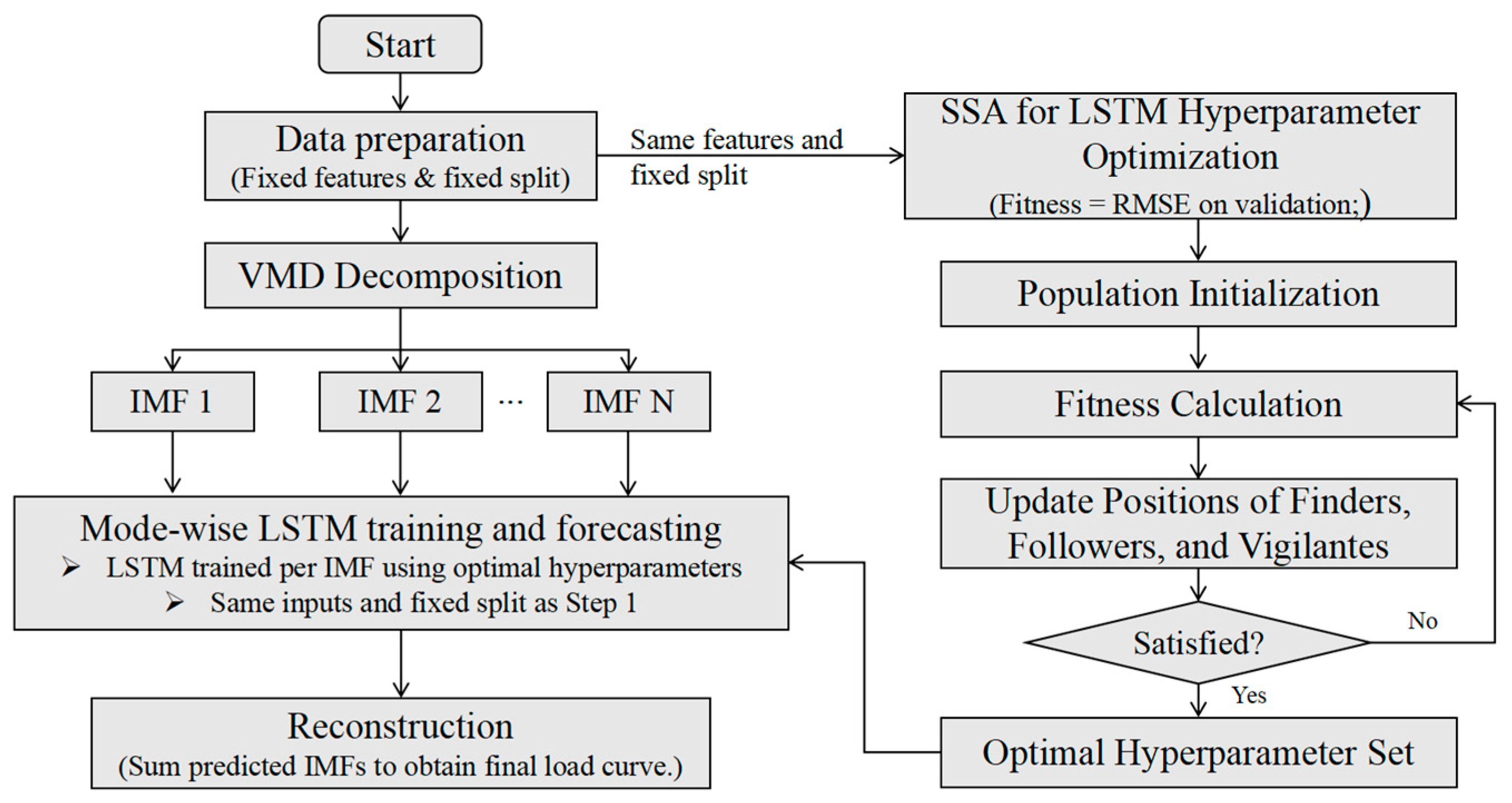
Building on the preceding analyses of the LSTM, VMD, and the SSA, this study proposes an integrated VMD-SSA-LSTM model for cooling and heating load forecasting in office parks. The model implements dual-level optimization tailored to the multi-scale characteristics and high complexity of the load series. On the one hand, VMD is employed to adaptively decompose the raw load series into multiple IMFs, effectively separating short-term fluctuations, daily/weekly cycles, and long-term trends to reduce the difficulty of direct modeling. On the other hand, the SSA is utilized to globally optimize key LSTM hyperparameters (e.g., number of hidden units, training epochs, and learning rate), thereby enhancing model generalization and predictive accuracy. Through a “decomposition–optimization–prediction–reconstruction” workflow, the approach achieves coordinated improvements at both the feature and model levels.

Implementation steps are as follows:

• Step 1—Data preparation and split: Normalize the cooling/heating loads and the primary influencing factors; perform a chronological train/validation/test split and keep this split fixed for all subsequent training and evaluations to ensure distributional consistency and comparability.
• Step 2—Multi-scale decomposition: Apply VMD separately to the target load series in the training, validation, and test subsets to obtain the corresponding sets of IMF subsequences; keep the influencing factors in the model inputs time-aligned one-to-one with the original series and processed on the same scale.
• Step 3—Hyperparameter optimization on fixed data: Using the validation-set root mean square error (RMSE) as the fitness, perform a global search with the SSA over the predefined LSTM hyperparameter space (e.g., number of hidden units, learning rate, and maximum epochs) based on the fixed train/validation split from Step 1; each candidate is fitted on the training set and evaluated on the validation set, with early stopping and cross-validation to mitigate overfitting and randomness, yielding the optimal hyperparameter set.
• Step 4—Mode-wise training and forecasting: With the optimal hyperparameters from Step 3, train an LSTM for each IMF subsequence and produce per-IMF predictions on the test set; keep input features and data splits identical to Step 1 to ensure reproducibility and fair comparison.
• Step 5—Reconstruction and evaluation: Reconstruct the final cooling/heating load forecast curve by summing the IMF predictions according to the VMD principle and compute metrics such as the RMSE and MAPE; additionally, conduct residual autocorrelation and distribution diagnostics to assess robustness.

Evaluation metrics and visualization: To comprehensively assess performance, the RMSE and MAPE are adopted as quantitative indicators. Additionally, visualization and statistical diagnostics of the forecast curves and residuals—such as residual autocorrelation, skewness, and kurtosis—are recommended to examine the adequacy and stability of the model’s multi-scale fit. The overall workflow is illustrated in Figure 1.

2.3. Day-Ahead Optimal Scheduling Model for the Park-Level IES

After outlining the system architecture and modeling assumptions, this section systematically elaborates the mathematical modeling, optimization objectives, constraints, and solution methodologies for the scheduling problem in detail.

2.3.1. System Architecture and Modeling Assumptions

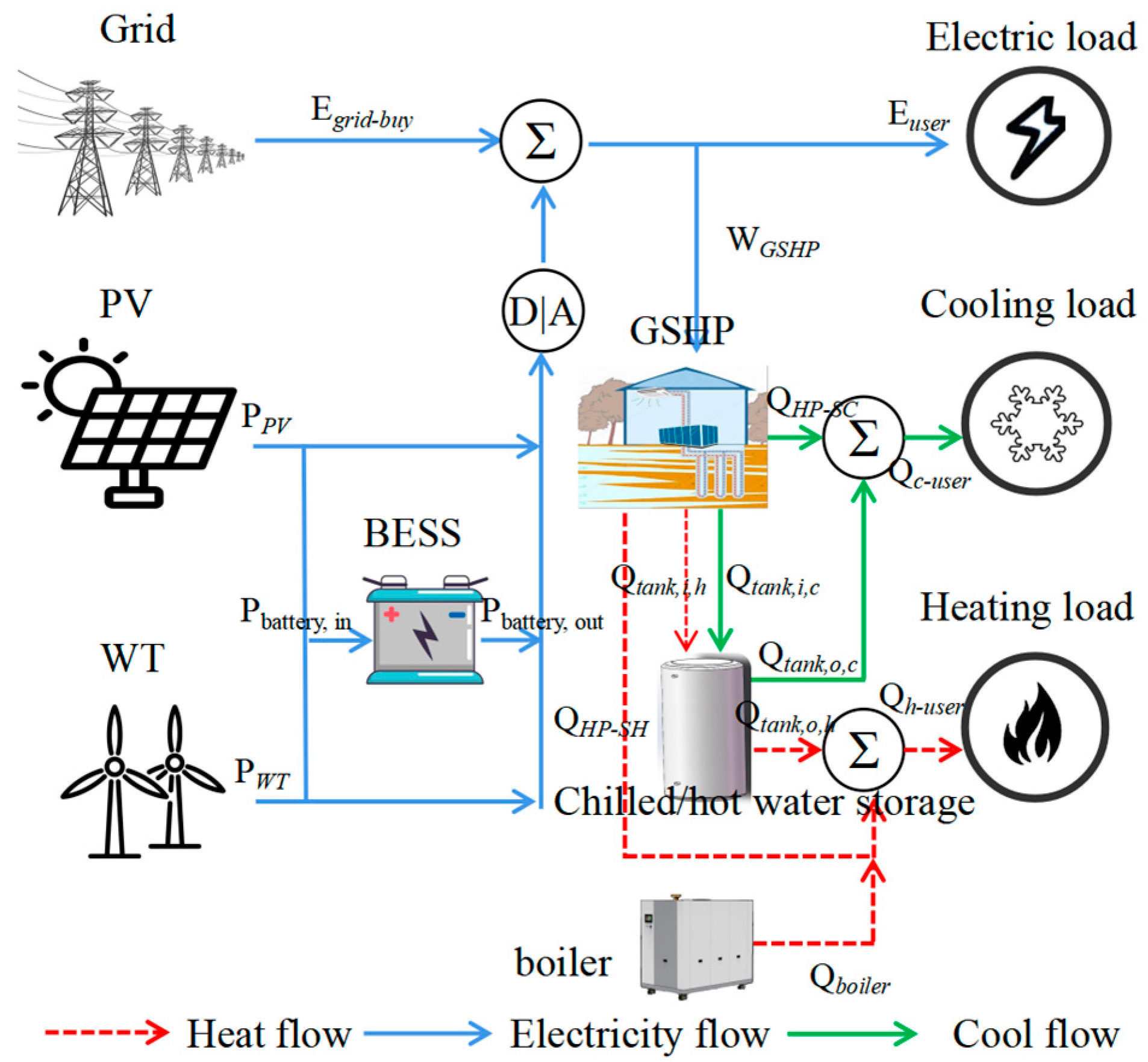
To achieve efficient energy utilization and emission reduction in office parks, a grid-connected IES is established, aligned with the trends of building electrification and clean, low-carbon energy. Unlike conventional combined cooling, heating, and power configurations that rely on steam turbines or diesel generator sets, the proposed system omits both diesel gensets and steam turbines. Electricity serves as the central energy carrier, integrating distributed renewable energy and multiple forms of energy storage. The system primarily comprises distributed PV generation, wind turbines (WTs), boilers, ground-source heat pumps (GSHPs), battery energy storage systems (BESSs), chilled/hot water storage tanks, and the utility grid. The system configuration is illustrated in Figure 2.

• System components and energy flow relationships

Electrical subsystem: Composed of PV, WTs, BESSs, and the utility grid. PV and wind generation are prioritized to meet park electrical loads. When renewable output is in surplus, it is first directed to charge the BESS; after the state of charge (SOC) reaches its upper bound, any remaining power is exported to the grid. When renewable output is insufficient, and except during off-peak tariff periods, BESS discharge is dispatched preferentially, with the remaining deficit supplied by grid purchases.

Cooling/heating subsystem: Cooling and heating are primarily provided by the GSHP, with the boiler supplying supplementary capacity to maintain year-round thermal balance, achieving source-side complementarity to accommodate seasonal demand fluctuations.

Chilled/hot water storage for peak shifting and intra-seasonal regulation: Storage is charged during nighttime low-tariff periods and discharged preferentially during daytime high-tariff periods to achieve peak shaving and valley filling.

Grid interaction: The IES exchanges power bidirectionally with the utility grid. Subject to interconnection codes, surplus electricity can be exported and real-time purchases can be made as needed. The system retains limited short-term islanding capabilities to enhance resilience and supply security.

2.

Operational strategies and dispatch principles

Priority consumption of renewable energy: PV and wind generation are first used to satisfy local demand; surplus electricity is then used for BESS charging and subsequently exported to the grid.

High-efficiency source-side operation: The GSHP is maintained, as far as possible, within the high-efficiency loading range of 80–100%, employing refined start–stop strategies and part-load control to balance energy efficiency with equipment life-cycle costs.

Power compensation order: During non-off-peak tariff periods, when renewable output is inadequate, BESS discharge is scheduled with priority; during off-peak periods, grid electricity is preferentially used to charge the BESS to enhance time-of-use arbitrage and reserve assurance.

Coordinated cooling/heating regulation: At night, the GSHP charges the chilled/hot water storage; during daytime peaks, stored energy is discharged with priority, with any remaining shortfall supplemented by the GSHP and boiler, respectively. This strategy aligns with engineering practice in terms of economic performance and operability.

3.

Modeling boundaries and key assumptions

System boundary: A grid-connected IES without diesel gensets or steam turbines, primarily consisting of PV, WTs, the utility grid, a BESS, boilers, a GSHP, and chilled/hot water storage tanks.

Time scale: A day-ahead rolling optimization framework is adopted with a 24 h horizon and a 1 h time step. Cooling/heating and electrical load forecasts are provided by the forecasting module described previously.

Data and parameters: Electricity prices follow time-of-use market tariffs; renewable generation is estimated based on meteorological data and component/unit models; equipment efficiencies are specified according to rated and part-load characteristics.

Physical constraints: Energy conservation; mutual exclusivity of storage charging/discharging with power and SOC bounds; source-side equipment power limits, minimum on/off times, and ramp-rate constraints; and capacity and heat-exchange power limits for chilled/hot water storage.

These architectural choices and assumptions are consistent with practical park-level integrated energy management. While ensuring supply security and thermal comfort, the coordinated effects of renewable priority consumption, storage-based peak shifting, and high-efficiency source-side operations enhance economic performance, energy efficiency, operational resilience, and provide clear boundary conditions and strategic foundations for the subsequent day-ahead optimal scheduling objective function and constraint formulation.

In summary, by performing multi-scale decoupling at the signal level and hyperparameter optimization at the model level, the VMD-SSA-LSTM framework effectively addresses the temporal complexity and variability of office park cooling and heating loads. It significantly improves forecasting accuracy and robustness, providing efficient and reliable technical support for optimal scheduling and operational management of IESs in office parks.

2.3.2. Mathematical Model

For the park-level integrated energy system considered in this study, the models for PV generation, WT generation, the BESS, and chilled/hot water thermal storage are adopted from well-established conventional modeling frameworks reported in the literature, and their detailed formulations are therefore omitted here for brevity. Given the pronounced influence of source-side equipment on day-ahead optimization results, particular attention is devoted to the GSHP. Its representation follows a data-driven modeling approach documented in a prior study [31], which explicitly distinguishes between two operational modes: direct supply to buildings and storage-oriented operation. This distinction enhances physical consistency and facilitates seamless integration with dispatch optimization models. The thermodynamic performance of the GSHP, including energy consumption, capacity, and part-load characteristics, is characterized in accordance with the ASHRAE handbook [33]. The complete mathematical derivation, parameterization, and validation of the GSHP model are comprehensively detailed in the cited reference [31] and are not reproduced herein.

2.3.3. Objective Functions

In the operational scheduling of the office park-level IES, targeted objective functions are proposed and defined for different interaction modes. First, to address the stability requirements of grid interaction, an external power-purchase smoothing objective is set, focusing on minimizing the SD of purchased power to reduce impacts on the upstream grid and enhance park-side regulation capabilities and grid-friendliness [34]. Second, to meet the requirement of economically optimal operation, the OC minimization objective is defined [32]. By leveraging time-of-use tariffs and storage-based peak shifting, the charging/discharging strategies of end-use units and storage units are coordinated to achieve cost savings and maximize overall benefits.

$$minSD=min\left\{\sqrt{{\displaystyle \frac{1}{24-1}}\sum _{t=1}^{24}{(E_{grid-buy}\left(t\right)-\overline{E_{grid-buy}\left(t\right)})}^2}\right\}$$

(3)

where $E_{grid-buy}\left(t\right)$ denotes the hourly external power purchase, kWh and $\overline{E_{grid-buy}\left(t\right)}$ denotes the average external power purchase, kWh.

$$minOC=min\left\{\sum _{t=1}^{24}\left(E_{grid-buy}\left(t\right)\times E_{grid}\left(t\right)\right)\right\}$$

(4)

where $E_{grid}\left(t\right)$ denotes the electricity price, ¥/kWh.

2.3.4. Constraints

To ensure physical consistency, safety bounds, and implementability of the optimization model for the office park-level IES, this study constructs a constraint set covering energy balance, storage device operation, and operating boundary conditions, and provide corresponding solution strategies. At the constraint level, this study follows the full “source–grid–load–storage” energy conservation principle, and, together with device efficiency and capacity limits, forms a mathematical model suitable for day-ahead rolling optimization.

• System energy balance constraints

For each discrete time period, balance relationships are established separately for electricity, cooling, and heating energy flows to guarantee dynamic supply–demand matching and stable system operation.

Electrical balance: At any time, the total supply power from PV generation, grid-purchased electricity, and battery discharging should equal the total demand from the GSHP power, chiller power, transmission/distribution and terminal electricity consumption, other building electricity uses, battery charging power, and curtailed wind/PV exports. The balance relationship is described as follows:

$$\begin{gathered} P_{PV}\left(t\right)+P_{WT}\left(t\right)+P_{boiler}\left(t\right)+P_{battery,in}\left(t\right){\eta }_c\Delta t+E_{grid-buy}\left(t\right) \\ \hspace{1em}\hspace{1em}\hspace{1em}\hspace{1em}\hspace{1em}\hspace{1em}\hspace{1em}\hspace{1em}\hspace{1em}\hspace{1em}=(1+\beta )\times W_{GSHP}\left(t\right)+E_{user}\left(t\right)+P_{battery,out}\left(t\right)\Delta t/{\eta }_d \end{gathered}$$

(5)

Here, P_PV is the PV system generation, kWh; P_WT is the WT system generation, kWh; P_boiler denotes the boilers’ electrical power consumption kWh; P_battery,in(t) is the battery charging power, kW; η_c is the charging efficiency, set to 0.9; $W_{GSHP}$ denotes GSHP energy consumption over the time interval, kWh; P_battery,out(t) is the battery discharging power, kW; η_d is the discharging efficiency, set to 0.9; and β is set to 30%, representing the ratio coefficient of transmission/distribution and terminal system power to the GSHP’s energy consumption. P_boiler denotes the boiler’s electricity consumption, kWh; E_grid-buy is the electricity purchased from the grid, kWh; E_user represents the user’s electrical load, kWh; and ∆t is the charging or discharging time, h.

Under heat-storage and heat-release operating modes, the GSHP heat production and the thermal storage tank charge/discharge must jointly satisfy the building heat load, while accounting for tank thermal losses and end-side heat-exchange losses:

$$N\times Q_{HP-SH}\left(t\right)\times PLR+Q_{tank,o,h}\left(t\right)+Q_{boiler}\left(t\right)=Q_{h-user}\left(t\right)+Q_{tank,i,h}\left(t\right)$$

(6)

where Q_HP-SH is the heat produced by the GSHP, kW; N denotes the number of units in operation; Q_boiler is the boiler’s heat output, kW; Q_tank,o,h is the heat supplied by the thermal storage tank, kW; Q_tank,i,h is the heat stored in the thermal storage tank, kW; and PLR is the part-load ratio.

Cooling supply balance: Under cold-storage and cold-release modes, the cooling produced by the GSHP or chiller together with the charge/discharge of the chilled-water tank jointly meets the building cooling load, with tank cold-energy losses taken into account.

$$N\times Q_{HP-SC}\left(t\right)\times PLR+Q_{tank,o,c}\left(t\right)=Q_{c-user}\left(t\right)+Q_{tank,i,c}\left(t\right)$$

(7)

where Q_HP-SC is the cooling capacity by the GSHP, kW; Q_c-user is the park’s cooling load, kW; Q_tank,o,c is the cold supplied by the cold storage tank, kW; and Q_tank,i,c is the cold stored in the cold storage tank, kW.

The above balance equations ensure consistent conservation of the three energy flows—electricity, cooling, and heating—over each time interval, thereby providing the basis for stable operation of the IES.

2.

Storage device operation and boundary constraints

Battery operation constraints: The SOC must always be kept between the maximum and minimum thresholds to strictly prevent overcharge or overdischarge. The SOC time evolution must consider physical parameters such as self-discharge rate, charge/discharge efficiency, and capacity. Only one operating mode—charging or discharging—is allowed at any time, and the corresponding charge/discharge power must not exceed the rated maximum:

During charging and discharging, the battery must satisfy constraints given by Equations (8) and (9).

$$\left\{\begin{array}{c}{SOC}_{min}\le SOC\left(t\right)\le {SOC}_{max}\\ 0\le P_{battery,in}\le P_{battery,in,max}\\ 0\le P_{battery,out}\le P_{battery,out,max}\end{array}\right.$$

(8)

$$\left\{\begin{array}{c}{P}_{battery,in}\left(t\right)\times P_{battery,out}\left(t\right)=0\\ P_{battery,in}\left(t\right)\ge 0\\ P_{battery,out}\left(t\right)\ge 0\end{array}\right.$$

(9)

where P_{battery,in,max} and P_{battery,out,max} are the maximum battery charging and discharging power ratings, kW.

Chilled/hot water tank operation constraints: The energy stored in the chilled/hot water tank must remain balanced, cannot exceed the physical capacity upper limit, and must stay nonnegative. The energy evolution of the tank, besides charge/discharge operations, should also account for thermal losses and charge/discharge efficiencies. System scheduling allows only one operating mode—charging or discharging—at any time, and the charge/discharge power must not exceed its upper limit:

$$0\le Q_{tank}\left(t\right)\le Q_{tank,max}\left(t\right)$$

(10)

$$\left\{\begin{array}{c}{P}_{tank,i}\left(t\right)\times P_{tank,o}\left(t\right)=0\\ P_{tank,i}\left(t\right)\ge 0\\ P_{tank,o}\left(t\right)\ge 0\end{array}\right.$$

(11)

where Q_tank(t) is the chilled or hot energy stored at time t, kW; Q_tank,max is the rated capacity of the chilled/hot water tank, kW; P_tank,i is the power consumed during charging, kW; and P_tank,o is the power consumed during discharging, kW. To ensure rational energy utilization, the optimization constrains the chilled/hot water tank to charge only during valley-price periods and enforces day-long conservation between stored and released energy, i.e., balancing total storage input and output over the day.

2.3.5. Solution Methodology

This study implements the numerical solution of the optimal scheduling model by integrating the Gurobi commercial solver on the Matlab R2018b platform. Gurobi efficiently handles complex problems such as linear programming and mixed-integer programming, with built-in simplex and interior-point methods, branch-and-bound, branch-and-cut, and various heuristics, thereby meeting the solution requirements of the park-level IES that involves discrete start–stop decisions and mutual-exclusion logic.

Given the mixed-integer programming nature of the proposed model, this study adopts a branch-and-bound framework as the core, augmented with pruning and heuristic acceleration. The overall procedure is summarized as follows:

• Problem relaxation: Relax integer variables to continuous ones and solve the linear relaxation to obtain a lower bound on the objective; if the relaxed solution satisfies integrality, it is directly returned as the global optimum.
• Branching strategy: For variables that violate integrality in the current solution, perform binary (or multi-way) branching to construct subproblems, recursively partitioning the decision space.
• Bounding and incumbent update: Solve the relaxed models of the subproblems to obtain lower bounds; if a feasible integer solution is found, update the current best upper bound and record the corresponding solution.
• Pruning criterion: Prune and discard a subspace when its lower bound is no smaller than the incumbent upper bound, or when the model is deemed infeasible.
• Iterative convergence: Continue branching, bounding, and pruning to shrink the feasible region until all subproblems are solved or pruned, yielding a global optimum or a solution within the prescribed optimality tolerance.

With this methodology, Gurobi can efficiently handle diverse constraints and coupled variables, delivering a globally optimal scheduling scheme for the park-level IES, thereby improving economic performance and operational stability while enhancing energy allocation and utilization efficiency.

3. Case Study

3.1. Overview of the Park

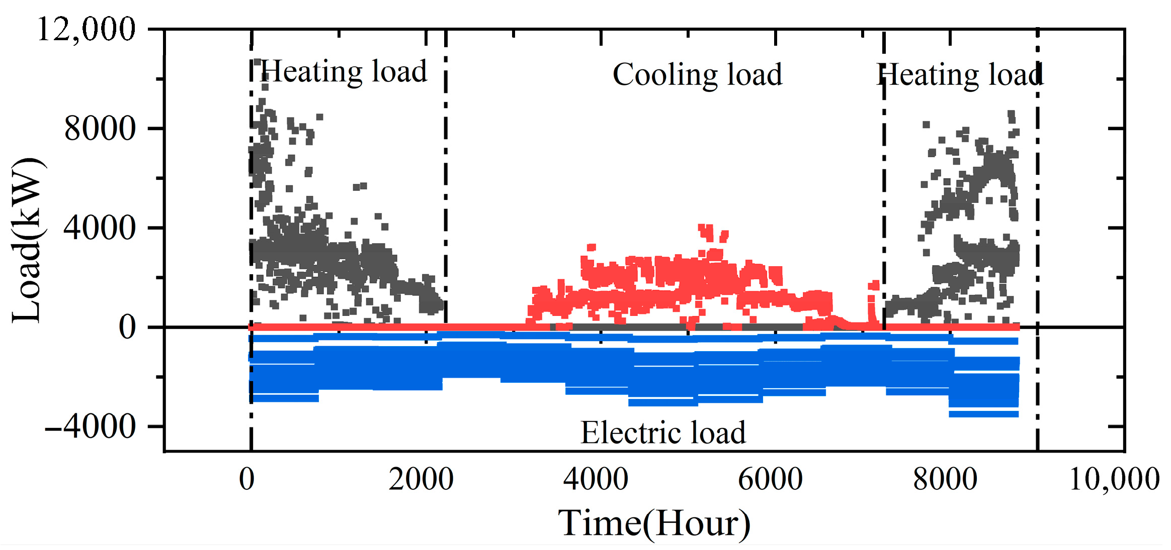
This study selects a certain office park in Tianjin as the object of optimization scheduling for the park-level IES. The park covers a total building area of about 160,000 square meters, including 12 office buildings, 2 dormitories, and 1 canteen, with diverse functions and complex energy-use characteristics. The energy system integrates multiple renewable and high-efficiency energy-using devices: a rooftop PV system with an installed capacity of 2000 kWp; a wind power system with a capacity of 600 kW connected to the grid at 380 V for on-site consumption, with surplus power not connected to the grid; three electric screw chiller–geothermal heat pump units with a heating capacity of 1300 kW each, providing the main assurance for winter heating and summer cooling; and two boilers with a heating capacity of 1000 kW to supplement heating and maintain a year-round soil thermal balance. The park also features a total energy storage capacity of 4000 kWh (located in the basement microgrid control room and the battery room) and 2200 m³ of cold/hot storage water tanks, forming a comprehensive energy system with multi-energy complementarity and flexible regulation for heating, cooling, and electricity. Relying on the energy consumption monitoring system, the park achieves real-time monitoring of hourly electricity loads for the year, and the inlet/outlet water temperatures and flow rates of the geothermal heat pumps, thereby obtaining hourly heating, cooling, and electrical loads, as shown in Figure 3. Monitoring results indicate that the annual cooling load totals 4952 MWh, with a peak cooling load of 4017 kW; the annual heating load totals 9316 MWh, with a maximum heating load of 10,694 kW; and the electrical load remains relatively steady throughout the year, with a peak of 3498 kW.

3.2. Parameter Settings

To comprehensively evaluate the effectiveness of the VMD-SSA-LSTM cooling load forecasting model, this study conducts a systematic comparison with several mainstream load forecasting methods. The comparison models include the following: Support Vector Machines (SVMs), Artificial Neural Networks (BPs), SVMs optimized by the ABC algorithm (ABC-SVM), SVMs optimized by Genetic Algorithms (GA-SVM), SVMs optimized by Particle Swarm Optimization (PSO-SVM), and a Wavelet-decomposed SVM (Wavelet-SVM). These choices are highly representative and cutting-edge. The key parameters for each model are set according to the algorithmic mechanism and prior hyperparameter tuning results; see

Table 3. Technical parameters of various prediction algorithms [35,36,37,38].

Algorithm Type	Parameter Description	Parameter Setting
VMD	Modal number K	5
	Penalty factor	2500
SSA	Population size	30
	Maximum number of iterations	10
	Alert threshold	0.6
	Proportion of watchdogs	0.2
	Proportion of explorers	0.7
LSTM	Number of hidden units	300
	Maximum training epochs	300
	Initial learning rate	0.072
ABC	Number of food sources	50
	Iterations	500
GA	Population size	100
	Maximum evolution generations	200
PSO	Population size	100
	Maximum evolution generations	200
	Local search intensity c1	1.5
	Global search intensity c2	1.5
Wavelet	Wavelet basis function	db4
	Decomposition level	3
SVM	Penalty parameter c	0.01–1000
	Kernel parameter g	0.01–1000
BP	Number of hidden neurons	7

for details. In the ensemble modeling framework, VMD parameters are determined by a two-stage grid search with joint criteria: K is searched over 3–10 (step 1) and α over 100–5000 (step 100). For each candidate pair, the reconstruction error surface and a composite modal-quality score are evaluated. Errors rise rapidly in the region K < 5 and α > 2500 (mostly >50, up to ~150), while remaining below 50 elsewhere. The modal-quality score increases monotonically with α, indicating reduced inter-mode overlap and improved independence. Balancing both criteria yields K = 5 and α = 2500, ensuring robust decomposition and best or near-best forecasting accuracy. Meanwhile, the SSA is employed to perform a global search and optimization of the three core LSTM hyperparameters (number of hidden units, maximum training epochs, and initial learning rate), yielding the optimal model structure and parameter configuration for predicting office park air-conditioning loads, and ensuring strong performance in accuracy and generalization.

Time-of-use electricity pricing is employed. Based on the electricity usage periods, prices are divided into Peak, Flat (Shoulder/Standard), and Off-Peak periods. Detailed standards are shown in

Table 4. Technical parameters of various prediction algorithms.

Period	Price (RMB/kWh)	Time Range
Peak	0.9175	09:00–12:00, 16:00–21:00
Flat	0.6435	07:00–09:00, 12:00–16:00, 21:00–23:00
Off-Peak	0.3815	23:00–07:00

.

4. Case Analysis and Discussion

4.1. Results and Analysis of the Load Forecasting Model

To systematically evaluate the contribution of load forecasting to the operation optimization of park-level IES, this section first starts from data correlations to quantify and identify the main influencing factors and temporal dependency features of cooling and heating loads, ensuring the scientificity and interpretability of input features. Subsequently, under unified data partitioning and evaluation metrics, it compares the accuracy and robustness of multiple mainstream forecasting models, examining the effectiveness and relative advantages of the “decomposition–reconstruction + deep learning” framework.

4.1.1. Correlation Analysis

As shown in Figure 4, panel (a) presents the Pearson correlation matrix for the cooling load of the office park, while panel (b) provides the corresponding analysis results for the heating load. The results indicate that for both cooling and heating loads, historical air-conditioning loads (e.g., L_t-24, L_t-48, L_t-72) exhibit the strongest correlation with the current load L, with correlation coefficients all exceeding 0.50. In particular, the correlation between L_t-24 and the cooling load is nearly 0.70, and reaches 0.81 for the heating load, highlighting the strong inherent temporal dependence of air-conditioning load data. Temperature-related variables (e.g., T_o, T_t-1, T_t-2, T_t-3, T_max, T_min, and T_av) show correlation coefficients mostly ranging from 0.30 to 0.55, indicating a clear influence of ambient temperature on load variation. Relative humidity and its lag terms (RH, RH_t-24, RH_t-48, and RH_t-72) exhibit weaker yet non-negligible correlations—approximately 0.17–0.21 for cooling and about 0.12–0.17 for heating. Although these variables are less influential than temperature and historical load, they still provide auxiliary explanatory power. In contrast, the weekday indicator (W_k) shows an almost zero correlation with cooling load and only a weak correlation with heating load, while the time-of-day feature (t) demonstrates a moderate negative correlation with cooling and a slight positive correlation with heating, suggesting limited effects from these temporal descriptors.

In summary, a systematic multivariate correlation analysis for the office park indicates that historical air-conditioning load, temperature variables, and relative humidity are the primary drivers of load variation. Accordingly, input features for load forecasting models should prioritize temperature, relative humidity, and historical load data to ensure that the models capture the core determinants of load dynamics and thereby improve predictive accuracy.

4.1.2. Load Forecasting Comparison

In the efficient operation of the park-level IES, load forecasting plays a foundational and strategic role. The temporal variability and uncertainty of load directly influence dispatch decisions and resource allocation. Historically, the previous day’s load curve has often been used as the dispatch baseline. As shown in Figure 5, in both heating and cooling seasons, daily load curves exhibit significant fluctuations and shifts in peak and off-peak periods. Comparisons of three consecutive days’ loads during heating and cooling seasons reveal that, although the overall trend is similar, peak and trough periods show pronounced fluctuations, with maximum deviations reaching 150% and average deviations reaching 35%. This level of uncertainty implies that continuing to rely on traditional dispatch strategies based on conventional daily loads would likely degrade actual dispatch performance, reduce system energy efficiency, and impair economic benefits, failing to reflect the potential and advantages of the park’s multi-energy complementary IES. Therefore, improving load forecasting accuracy is a prerequisite and key to optimizing system operation. High-precision load forecasting not only helps to anticipate intraday and daily load trends for day-ahead scheduling and real-time tuning, providing a scientific basis for operations, but also effectively responds to dynamic load curve changes to achieve precise matching of energy supply and demand.

Based on the above understanding, to validate the applicability and forecasting accuracy of the cooling/heating load prediction model under actual operating conditions, this study combines project-measured operational data to conduct systematic modeling and comparative analysis. In the data processing phase, load data samples are scientifically partitioned: a summer week and a winter week of hourly monitoring data are used as the training set, with the immediately following day’s hourly data used as the test set to ensure representative data distribution and temporal continuity for model training and validation. Based on correlation analysis results, the model inputs are strictly selected as temperature, relative humidity, and historical heating/cooling loads, with the output being the current heating/cooling load. This design robustly supports subsequent training and evaluation of high-precision load forecasting models and lays a solid foundation for optimizing the operation of the park-level IES.

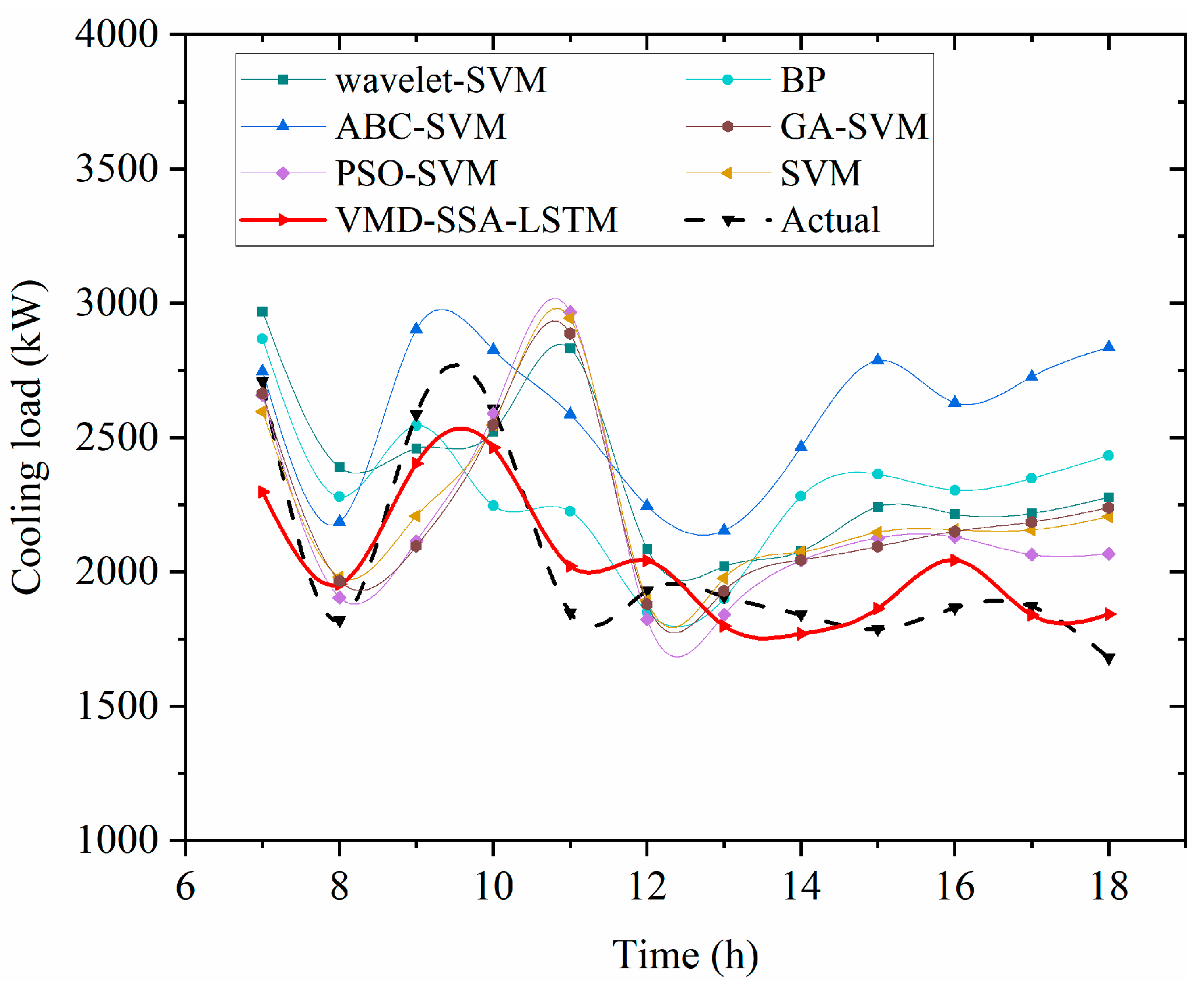
The cooling load prediction results are shown in Figure 6, where the prediction performances of several mainstream load forecasting models on the same dataset are visually compared. The figure indicates that the VMD-SSA-LSTM model most closely tracks the actual load fluctuations and effectively captures the volatility characteristics. The errors for each model were quantified and summarized in

Table 5. Error analysis of cooling load prediction results for the office park.

Prediction Algorithm	MAPE (%)	RMSE (kW)
ABC-SVM	28.64	401.07
GA-SVM	15.56	253.92
PSO-SVM	14.53	252.47
BP	19.11	266.43
Wavelet-SVM	18.82	270.52
SVM	15.58	256.45
VMD-SSA-LSTM	8.32	134.58

. The VMD-SSA-LSTM model achieves a MAPE of 8.32% and an RMSE of 134.58 kW for office park cooling load prediction, outperforming conventional methods such as the ABC-SVM, GA-SVM, and BP. This demonstrates the model’s structural advantages and learning capability in handling complex nonlinear time-series data.

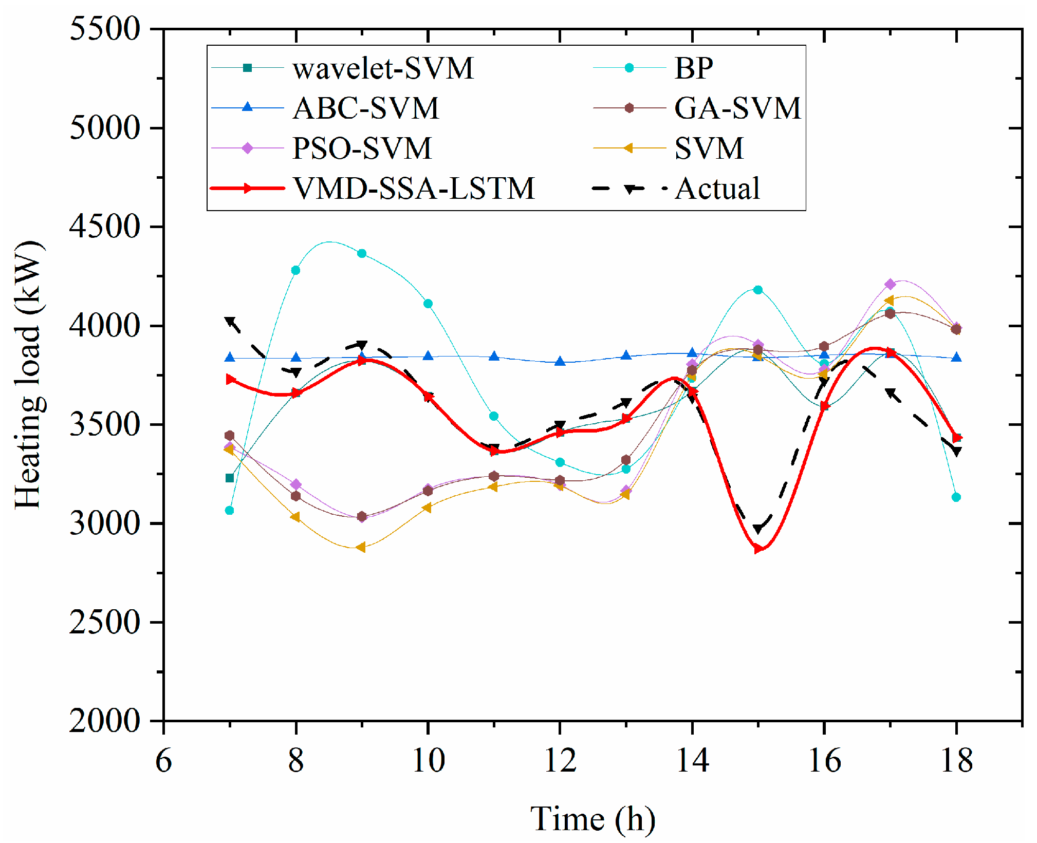
Figure 7 shows the results of heating load prediction models for the office park: hourly predictions vs. measurements on the test set, where the VMD-SSA-LSTM better captures peaks, valleys, and fluctuations. Error analysis (

Table 6. Error analysis of heating load prediction results for the office park.

Prediction Algorithm	MAPE (%)	RMSE (kW)
ABC-SVM	8.36	359.58
GA-SVM	13.58	550.36
PSO-SVM	14.03	558.50
BP	11.81	527.49
Wavelet-SVM	6.10	357.34
SVM	14.49	590.32
VMD-SSA-LSTM	5.8	229.74

) indicates that the VMD-SSA-LSTM achieves the best MAPE and RMSE, demonstrating stronger generalization and error convergence. Incorporating multi-source factors (temperature, relative humidity, and historical load) with a decomposition–reconstruction plus deep learning framework effectively improves cooling/heating load forecasting accuracy and supports energy management and optimal scheduling.

4.2. Day-Ahead Scheduling Optimization: Results and Analysis

In the practical operation of the park-level IES, a common pre-optimization practice is to adopt the previous day’s load curve as the control strategy for the current day. Although simple to implement, this approach is vulnerable to uncertainties such as weather and holidays, which often induce substantial fluctuations in energy demand between consecutive days. As a result, relying solely on historical load curves can lead to reduced energy efficiency and increased operating costs. In both heating and cooling seasons, directly applying the prior day’s load curve fails to address peak–valley shifts and abrupt amplitude changes, thereby limiting the potential of multi-energy complementarity and flexible regulation in IES.

In the day-ahead optimization analysis, this study systematically compares two scheduling strategies. The baseline strategy adopts the previous day’s load curve directly as the basis for current scheduling and equipment control. The optimized strategy leverages high-accuracy load forecasts (e.g., VMD-SSA-LSTM) as the core control reference. Two quantitative objectives related to grid interaction are considered as follows:

• Ensuring stable system operation to reduce the park’s impact on the grid;
• Assisting the grid in peak shaving and valley filling, optimizing the energy-use structure, and lowering operating costs.

For illustration, three representative days in both the cooling and heating seasons are randomly selected. Under the two strategies, the hourly operating states of key devices (e.g., GSHP, thermal storage tanks, and batteries) and the purchased electricity profiles are compared in detail.

4.2.1. Heating Season Analysis

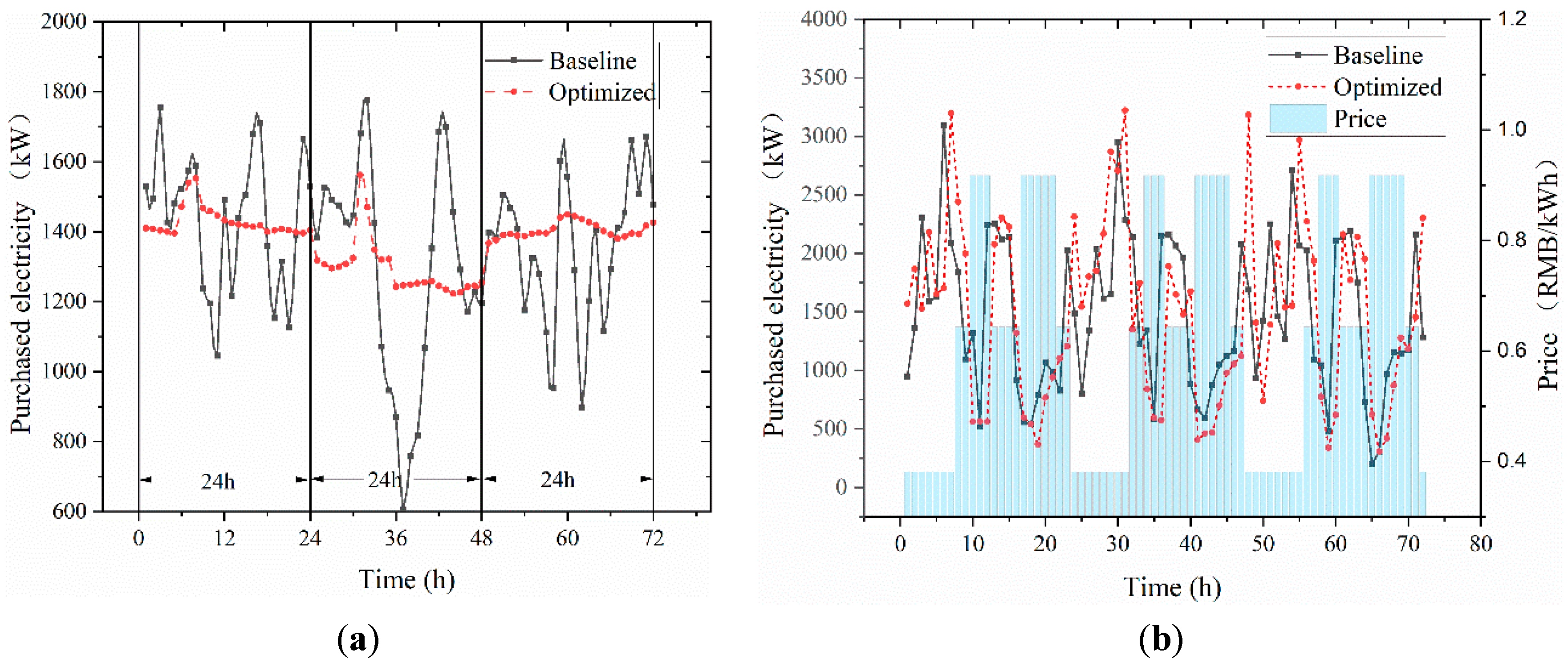
When the objective is to reduce the standard deviation of purchased electricity and achieve stable consumption, the baseline strategy—directly adopting the previous day’s load curve—results in large fluctuations in purchased power, particularly during the 08:00–22:00 peak period. These fluctuations primarily arise from the suboptimal scheduling of heat pump power use and battery charging/discharging. In certain hours, forecast errors lead to excessive discharge of chilled/hot-water storage, necessitating additional operation of the GSHP, while PV and wind deviations further disrupt battery dispatch. In contrast, the forecast-guided day-ahead scheduling precisely matches load variations and effectively smooths purchased electricity. For three representative days, the standard deviations of purchased electricity after optimization are only 44.6 kW, 82.7 kW, and 23.8 kW, far below the baseline values of 108.8 kW, 117.6 kW, and 130.95 kW, as shown in Figure 8.

When the goal is to assist grid peak shaving and reduce system operating costs, the total purchased electricity changes little before and after optimization; the main differences lie in the electricity consumption of the GSHP. By accurately controlling the chilled/hot-water storage, the optimized strategy improves heat pump efficiency, reducing daily operating costs by 6.4–15.1%. Although the percentage savings are modest, they provide tangible economic benefits for large-scale parks.

4.2.2. Cooling Season Analysis

When the objective is to reduce the standard deviation of purchased electricity, the traditional control strategy that directly adopts the previous day’s load curve leads to severe fluctuations in purchased power during 08:00–22:00. The primary causes are the improper release of cooling from chilled/hot-water storage due to load forecast errors, frequent operational changes in the ground-source heat pump, and disordered battery charging/discharging induced by PV and wind output deviations. In contrast, forecast-based day-ahead scheduling significantly enhances the anticipation of load variations, optimizes the operation of storage devices and cold/heat sources, and reduces volatility in purchased electricity. As shown in Figure 9, for three representative days, the standard deviations of purchased electricity after optimization are only 41.5 kW, 77.0 kW, and 22.7 kW, far better than 194.2 kW, 318.7 kW, and 202.9 kW under the traditional strategy, indicating a clear improvement in consumption stability.

When the goal is to assist the grid in peak shaving and reduce operating costs, the total purchased electricity changes little before and after optimization; however, the post-optimization operation of the ground-source heat pump and cold storage is more rational. The regulation of the chilled/hot-water storage avoids excessive release and improves heat pump efficiency. With forecast-assisted scheduling, system operating costs decrease by 3.8–11.6% compared with the baseline, yielding more pronounced savings than in the heating season.

Both the heating and cooling season analyses demonstrate that the proposed scheduling optimization method for the park-level IES—driven by thermal/electrical load forecasting and grid interaction—can markedly enhance the stability and economic performance of park-scale energy use. Compared with traditional strategies that rely solely on historical loads, the forecast-driven day-ahead scheduling not only substantially reduces fluctuations in purchased electricity but also effectively assists the grid in peak shaving and valley filling while lowering operating costs. This is evidence of superior multi-energy coordination and interaction capabilities, highlighting the method’s advancement and practical value for optimal dispatch in the park-level IES.

5. Conclusions

5.1. Main Findings

This article addresses the optimal scheduling of a park-level IES and proposes a scheduling optimization framework that integrates cooling/heating load forecasting with grid-interaction characteristics, followed by systematic validation. First, through a comprehensive correlation analysis between multiple influencing factors and the cooling/heating loads, historical load, ambient temperature, and relative humidity are identified as the primary drivers of load variation. Based on this insight, a high-accuracy load forecasting model is constructed using temperature, relative humidity, and historical load as inputs. The results show that advanced data-driven methods such as the VMD-SSA-LSTM can markedly improve the accuracy of cooling/heating load forecasting. The MAPE for the office park is 8.32% for cooling load and 5.8% for heating load, both outperforming conventional methods

Building on the forecasts, two day-ahead scheduling strategies—one based on historical load curves and the other on forecasted loads—are analyzed and compared. In representative heating and cooling season case studies, the forecast-driven optimization strategy exhibits a clear advantage, reducing the standard deviation of purchased electricity by 29.6–88.1%. Specifically, in the heating season, the post-optimization standard deviations for three representative days are 44.6 kW, 82.7 kW, and 23.8 kW, substantially lower than the pre-optimization values of 108.8 kW, 117.6 kW, and 130.95 kW. In the cooling season, the corresponding post-optimization values are 41.5 kW, 77.0 kW, and 22.7 kW, compared with 194.2 kW, 318.7 kW, and 202.9 kW before optimization. Moreover, forecast-based scheduling yields system operating cost savings of 6.4–15.1% in the heating season and 3.8–11.6% in the cooling season.

In summary, this work demonstrates that the proposed optimization framework—grounded in cooling/heating load forecasting and grid interaction—significantly enhances the stability, economic performance, and flexibility of the park-level IES. The method effectively addresses scheduling challenges arising from multi-energy coordination and load uncertainty, and it shows strong potential for engineering deployment and academic innovation. It provides a solid theoretical foundation and practical reference for the optimal dispatch of future park-level IESs.

5.2. Limitations and Future Work

Despite the encouraging results, several limitations remain. First, the current simulation model of the IES provides an insufficient representation of the thermal network and thus does not fully capture the complexity of energy transfer and coupling processes in real applications. Second, the load and equipment outputs are modeled with a one-hour time step and directly in terms of power, neglecting the delay and hysteresis effects inherent in cooling and heating systems. Future work should incorporate refined modeling of energy network inputs/outputs and transport characteristics to improve simulation fidelity. Third, the constraints on energy balance, energy supply, and device operation in the optimization model are relatively simplified and do not comprehensively cover the diverse constraints of multi-type supply equipment and thermal/electrical networks. Subsequent research should further refine model boundaries and constraint formulations to better align with the operational requirements of real systems.

References

1. International Energy Agency (IEA). Net Zero by 2050: A Roadmap for the Global Energy Sector; IEA: Paris, France, 2021. [Google Scholar]
2. Boukaf, M.; Fadli, F.; Meskin, N. A Comprehensive Review of Digital Twin Technology in Building Energy Consumption Forecasting. IEEE Access 2024, 12, 187778–187799. [Google Scholar] [CrossRef]
3. Gilani, M.A.; Kazemi, A.; Ghasemi, M. Distribution system resilience enhancement by microgrid formation considering distributed energy resources. Energy 2020, 191, 116442. [Google Scholar] [CrossRef]
4. DOE of United States. GRID 2030. In A National Vision for Electricity’s Second 100 Years; Penny Hill Press: Damascus, MD, USA, 2003. [Google Scholar]
5. Government of Canada. Combining Our Energies: Integrated Energy Systems for Canadian Communities [EB/OL]. Available online: http://publications.gc.ca/collections/collection_2009/parl/xc49-402-1-1-01e.pdf (accessed on 10 January 2025).
6. Natural Resources Canada. Integrated Community Energy Solutions-a Roadmap for Action [EB/OL]. Available online: http://oee.nrcan.gc.ca/sites/oee.nrcan.gc.ca/files/pdf/publications/cem-cme/ices_e.pdf (accessed on 10 January 2025).
7. European Commission. The Fifth Framework Programme [EB/OL]. Available online: http://ec.europa.eu/research/fp5 (accessed on 22 December 1998).
8. European Commission. The Sixth Framework Programme [EB/OL]. Available online: http://ec.europa.eu/research/fp6 (accessed on 22 December 1998).
9. European Commission. The Seventh Framework Programme [EB/OL]. Available online: http://ec.europa.eu/research/fp7 (accessed on 22 December 1998).
10. Tokyo Gas. Challenge for the Future Society: Smart Energy Network [EB/OL]. Available online: http://www.tokyo-gas.co.jp/techno/challenge/002_e.html (accessed on 10 January 2025).
11. National Development and Reform Commission, National Energy Administration. Implementation Opinions on Promoting the Construction of Multi-Energy Complementary Integration and Optimization Demonstration Projects [EB/OL]. 2016. Available online: http://www.gov.cn/xinwen/2016-07/08/content_5089294.htm (accessed on 8 July 2016).
12. Chen, F.; Deng, H.; Chen, Y.; Wang, J.; Jiang, C.; Shao, Z. Distributed robust cooperative scheduling of multi-region integrated energy system considering dynamic characteristics of networks. Int. J. Electr. Power Energy Syst. 2023, 145, 108605. [Google Scholar] [CrossRef]
13. Wang, L.; Lin, J.; Dong, H.; Wang, Y.; Zeng, M. Demand response comprehensive incentive mechanism-based multi-time scale optimization scheduling for park integrated energy system. Energy 2023, 270, 126893. [Google Scholar] [CrossRef]
14. Zhang, G.; Niu, Y.; Xie, T.; Zhang, K. Multi-level distributed demand response study for a multi-park integrated energy system. Energy Rep. 2023, 9, 2676–2689. [Google Scholar] [CrossRef]
15. Pan, C.; Jin, T.; Li, N.; Wang, G.; Hou, X.; Gu, Y. Multi-objective and two-stage optimization study of integrated energy systems considering P2G and integrated demand responses. Energy 2023, 270, 126846. [Google Scholar] [CrossRef]
16. Dong, H.; Fang, Z.; Ibrahim, A.; Cai, J. Optimized operation of integrated energy microgrid with energy storage based on short-term load forecasting. Electronics 2021, 11, 22. [Google Scholar] [CrossRef]
17. Ge, L.; Li, Y.; Yan, J.; Wang, Y.; Zhang, N. Short-term load prediction of integrated energy system with wavelet neural network model based on improved particle swarm optimization and chaos optimization algorithm. J. Mod. Power Syst. Clean Energy 2021, 9, 1490–1499. [Google Scholar] [CrossRef]
18. Shang, Z.; He, Z.; Song, Y.; Yang, Y.; Li, L.; Chen, Y. A novel combined model for short-term electric load forecasting based on whale optimization algorithm. Neural Process. Lett. 2020, 52, 1207–1232. [Google Scholar] [CrossRef]
19. Huo, W.; Zhou, J. Power load prediction model based on long short term memory and sparrow search algorithm. J. Phys. Conf. Ser. 2021, 2022, 012018. [Google Scholar] [CrossRef]
20. Xue, J.; Shen, B. Dung beetle optimizer: A new meta-heuristic algorithm for global optimization. J. Supercomput. 2023, 79, 7305–7336. [Google Scholar] [CrossRef]
21. Huang, X.; Han, Y.; Yan, J.; Zhou, X. Hybrid forecasting model of building cooling load based on EMD-LSTM-Markov Algorithm. Energy Build. 2024, 321, 114670. [Google Scholar] [CrossRef]
22. Wang, J.; Zeng, A.; Wan, Y. Multi-Time-Scale Optimal Scheduling of Integrated Energy System Considering Transmission Delay and Heat Storage of Heating Network. Sustainability 2023, 15, 14260. [Google Scholar] [CrossRef]
23. Hossein, T.; Kazemi, A.; Shakouri, H.; Kocaman, A.S.; Caldwell, N. An integrated price- and incentive-based demand response program for smart residential buildings: A robust multi-objective model. Sustain. Cities Soc. 2024, 113, 105664. [Google Scholar]
24. Fan, W.; Tan, Q.; Zhang, A.; Ju, L.; Wang, Y.; Yin, Z.; Li, X. A Bi-level optimization model of integrated energy system considering wind power uncertainty. Renew. Energy 2023, 202, 973–991. [Google Scholar] [CrossRef]
25. Zhang, Y.; Zhang, X.; Ji, X.; Han, X.; Yang, M. Optimization of integrated energy system considering transmission and distribution network interconnection and energy transmission dynamic characteristics. Int. J. Electr. Power Energy Syst. 2023, 153, 109357. [Google Scholar] [CrossRef]
26. Ullah, K.; Khan, T.A.; Hafeez, G.; Khan, I.; Murawwat, S.; Alamri, B.; Ali, F.; Ali, S.; Khan, S. Demand Side Management Strategy for Multi-Objective Day-Ahead Scheduling Considering Wind Energy in Smart Grid. Energies 2022, 15, 6900. [Google Scholar] [CrossRef]
27. Pietro, R. A multi-agent framework for smart grid simulations: Strategies for power-to-heat flexibility management in residential context. Sustain. Energy Grids Netw. 2023, 34, 101072. [Google Scholar]
28. Wu, K.; Jiang, M.; Huang, Y.; Dai, Z.; Wang, X.; Duan, Z.; Wang, Y.; Li, G. Optimization of multi-objective capacity allocation and performance analysis for integrated energy systems considering hydrogen storage. Energy 2025, 325, 136160. [Google Scholar] [CrossRef]
29. Cga, C. Integrated planning of internet data centers and battery energy storage systems in smart grids. Appl. Energy 2021, 281, 116031. [Google Scholar] [CrossRef]
30. Mounir, N.; Ouadi, H.; Jrhilifa, I. Short-term electric load forecasting using an EMD-BI-LSTM approach for smart grid energy management System. Energy Build. 2023, 288, 113022. [Google Scholar] [CrossRef]
31. Zheng, L.; Wang, J.; Chen, J.; Ye, C.; Gong, Y. Two-Stage Co-Optimization of a Park-Level Integrated Energy System Considering Grid Interaction. IEEE Access 2023, 11, 66400–66414. [Google Scholar] [CrossRef]
32. Chen, S.; Zhao, L.; Zheng, L.; Bi, G. A rapid evaluation method for design strategies of high-rise office buildings achieving nearly zero energy in Guangzhou. J. Build. Eng. 2021, 44, 103297. [Google Scholar] [CrossRef]
33. Tang, H.; Yu, J.; Geng, Y.; Liu, X.; Lin, B. Optimization of operational strategy for ice thermal energy storage in a district cooling system based on model predictive Control. J. Energy Storage 2023, 62, 106872. [Google Scholar] [CrossRef]
34. Xu, X.; Ming, W.; Zhou, Y.; Wu, J. Unlock the flexibility of combined heat and power for frequency response by coordinative control with batteries. IEEE Trans. Ind. Inform. 2021, 17, 3209–3219. [Google Scholar] [CrossRef]
35. Huang, Q. Research on a VMD—SSA—LSTM Based Traffic Forecasting Model. Master’s Thesis, Shenyang Agricultural University, Shenyang, China, 2023. [Google Scholar]
36. Ding, Y.; Zhang, Q.; Yuan, T.; Yang, K. Model input selection for building heating load prediction: A case study for an office building in Tianjin. Energy Build. 2018, 159, 254–270. [Google Scholar] [CrossRef]
37. Ding, Y.; Zhang, Q.; Yuan, T.; Yang, F. Effect of input variables on cooling load prediction accuracy of an office Building. Appl. Therm. Eng. 2018, 128, 225–234. [Google Scholar] [CrossRef]
38. Sun, Q.; Cai, H. Short-Term Power Load Prediction Based on VMD-SG-LSTM. IEEE Access 2022, 10, 102396–102405. [Google Scholar] [CrossRef]
Figure 1. VMD-SSA-LSTM load forecasting model workflow diagram. Both SSA optimization and per-IMF training share identical inputs and fixed train/val/test split; the SSA uses validation RMSE as fitness.
Buildings 15 03920 g001
Figure 2. Energy flow diagram of the office park IES.
Buildings 15 03920 g002
Figure 3. Hourly load distribution and electrical load distribution in the park.
Buildings 15 03920 g003
Figure 4. (a) Pearson correlation coefficient results for the office park cooling load; (b) Pearson correlation coefficient results for the office park heating load.
Buildings 15 03920 g004
Figure 5. (a) Day-to-day comparison of heating load fluctuations; (b) day-to-day comparison of cooling load fluctuations.
Buildings 15 03920 g005
Figure 6. Predicted cooling load results of various models for the office park.
Buildings 15 03920 g006
Figure 7. Predicted heating load results of various models for the office park.
Buildings 15 03920 g007
Figure 8. Comparison of purchased electricity before and after optimization on three representative heating season days. (a) Reduce the standard deviation of purchased electricity to mitigate grid impact; (b) assist grid peak shaving and reduce operating costs.
Buildings 15 03920 g008
Figure 9. Comparison of purchased electricity before and after optimization on three representative cooling-season days. (a) Reduce the standard deviation of purchased electricity to mitigate grid impact; (b) assist grid peak shaving and reduce operating costs.
Buildings 15 03920 g009