Abstract
While urban green spaces are integral to urban resilience, their long-term dynamics under recurrent flooding have received limited scholarly attention. This study investigates two decades of green space change across 367 counties in the southeastern United States, integrating FEMA disaster records with multi-period land cover data. Employing generalized additive and logistic regression models, the impacts of flood frequency, development intensity, and socioeconomic drivers were assessed. Flood frequency was identified as the primary determinant of urban green space loss. Each additional flood event corresponded to a 0.36% reduction in the five-year green space change rate (p < 0.01), while extreme flood frequency (≥ 10 events) was associated with an 18-fold increase in the odds of long-term degradation. Development intensity exhibited a significant non-linear effect, with loss rates culminating at moderate-to-high intensities. Furthermore, household income functioned as a significant moderator; in extremely flood-prone areas, higher income correlated with enhanced resilience (OR = 0.155, p < 0.05). These findings demonstrate that recurrent floods function as a cumulative pressure. This research highlights the necessity of equitable green infrastructure planning that integrates flood risk with the complex, moderating role of socioeconomic capacity.
1. Introduction
Urban green spaces, as integral components of urban ecosystems, are widely regarded as key assets that play an irreplaceable role in providing ecosystem services and supporting urban resilience [1]. They not only mitigate flood risks, regulate urban microclimates, and enhance environmental quality [2], but also serve as a critical link between maintaining ecosystem stability and promoting human well-being [3,4]. However, under the backdrop of global climate change, green spaces face increasingly severe external threats. The rising frequency and intensity of natural disasters such as floods are directly impacting their structure and functions [5,6]. Acute environmental shocks such as single flood events or hurricanes cause immediate and visible damage. In contrast, chronic environmental stressors, including recurrent flooding and prolonged inundation, act over long periods and create gradual cumulative impacts on ecosystems and societies. This distinction is important for understanding how resilience develops and erodes over time. In this paper we do not interpret flooding as a single, direct cause of greenspace loss. Instead, recurrent floods are considered a chronic pressure that can interact with urban development. The relationship between flooding and green space is reciprocal: land-use change and deforestation increase flood risk, while repeated inundation—particularly in coastal and low-lying counties—can hinder vegetation recovery through saltwater intrusion, soil degradation, and reconstruction priorities. Inland events are more likely to affect green space indirectly via redevelopment dynamics rather than immediate physical destruction. This framing complements, rather than contradicts, the role of green infrastructure in mitigating floods. Recurrent flooding functions as a chronic hydrological pressure that slowly weakens the structure and recovery capacity of urban green spaces through repeated disturbance and recovery cycles [7,8]. At the same time, internal pressures driven by urbanization, such as continuous population growth and intensified land development [9], further encroach upon green space and represent long-term drivers of green space loss [10]. These external threats and internal pressures converge particularly in the southeastern United States, making it a representative region of urban green space vulnerability. This region has long been exposed to extreme weather events such as floods and hurricanes [11], while also undergoing rapid and sustained urban expansion [12], resulting in a highly complex risk landscape. Recent assessments indicate that climate change may substantially increase flood risks by the mid-21st century. These risks are distributed unevenly across spatial and social dimensions, concentrated especially along the Atlantic and Gulf coasts, and disproportionately affecting vulnerable populations [13]. Coupled with ongoing population growth and intensified land development, these dynamics may further amplify flood threats, thereby posing unprecedented challenges to the sustainability of regional green spaces [14,15].
Despite previous research on urban green space dynamics, existing studies still exhibit notable theoretical limitations. First, a dominant research stream has extensively documented the long-term evolution of urban green space, primarily linking its decline to anthropogenic drivers. Numerous studies attribute green space loss primarily to anthropogenic drivers such as urban expansion, land-use intensification, and socioeconomic development [16]. This focus, while valuable, has often led to the neglect of concurrent environmental stressors. For example, Lin et al. [17] analyzed how land use and housing density in Sydney reduced green space availability, yet their framework did not incorporate climate-related factors. Similarly, Wu et al. [18] examined green space dynamics in Changchun, concluding that changes were mainly driven by urbanization and policy while overlooking the role of long-term climatic pressures. Consequently, while the connection between urban development and green space change is well-established, the moderating or compounding influence of hydrological hazards like flooding remains poorly understood within this context.
Concurrently, some studies have examined the relationship between flooding and green space, but this line of work is constrained by two major shortcomings. The first is a predominant focus on acute, single-event impacts rather than chronic, cumulative stress [19,20].
For instance, Gupta and Dixit [21] assessed the relationship between urban green space proportions and flood susceptibility through a one-time flood vulnerability analysis, highlighting the flood-mitigating role of green space. Similarly, Saadatkhah et al. [22] used a hydrological model to evaluate the effect of land cover change during the extreme 2014 Kelantan flood in Malaysia, effectively capturing short-term hydrological responses to a single flood event but did not address the cumulative effects of recurrent inundation. This gap is critical, as it obscures the process by which frequent floods can act as a persistent pressure, progressively weakening green space systems.
The second shortcoming is the tendency to frame green space in a one-way causal relationship as a “remedy” for flooding, which neglects how repeated flood exposure functions as a long-term hydrological stress that systematically erodes the resilience of urban green space systems. This perspective highlights the capacity of green space to mitigate runoff [23,24] but overlooks the critical reciprocal interaction: frequent inundation can degrade vegetation and destabilize soil, thereby weakening the very protective functions that green spaces are expected to provide. For example, recent studies have conceptualized green infrastructure solely as a flood-management tool or focused exclusively on its benefits, without addressing the negative impacts of flooding on the green space systems themselves [25,26]. In addition, while prior work confirms that floodplains are among the world’s most threatened ecosystems, with their integrity degraded by human activities [27], there remains insufficient understanding of how long-term, high-frequency flood exposure interacts with urban development pressures and socioeconomic factors to shape county-level green space dynamics.
Beyond theoretical gaps, existing research on the relationship between urban green space and flooding is constrained by several methodological limitations. First, studies are often limited by a narrow analytical scope, typically relying on single case studies or extreme flood events confined to specific cities [28,29]. This approach limits spatial representativeness and the generalizability of findings, as it often lacks the cross-regional comparisons and multi-temporal dynamic tracking needed to identify long-term and recurrent flood–green space interactions [30]. For instance, the work of Gupta and Dixit [31] was limited by its cross-sectional design in a single region, while the study by Li et al. [32] offered insights for Beijing but could not capture broader spatial or long-term dynamics. Second, methodological approaches are frequently oversimplified, failing to capture the nonlinear dynamics of coupled social-ecological systems. Many studies rely on linear regression models applied to cross-sectional or limited time-point data, which cannot trace complex trajectories, threshold effects, or feedback mechanisms [33]. For example, Kim et al. [34] examined the relationship between NDVI and runoff using OLS regression across only two temporal snapshots, a static approach unable to uncover dynamic couplings under long-term conditions. Third, existing approaches remain insufficient in handling long-term time series data. Even when using datasets spanning two decades or more, analyses are often restricted to inter-period comparisons that lack systematic modeling of trend evolution [35]. This prevents the identification of dynamic long-term couplings and overlooks the evolving influence of climatic and socioeconomic drivers [36]. For instance, Luo and Zhang [37] identified a declining trend in flood regulation services in China, their analysis did not account for these temporal dependencies, thereby limiting its ability to reveal the nonlinear evolution of flood risks. Finally, current frameworks often fail to integrate the complex interactions among flooding, green space, and socioeconomic factors. Even advanced approaches like multi-objective optimization are often applied to static scenarios in single case studies, neglecting how social dimensions like population density, income, and vulnerability dynamically shape flood risk. These methods have a limited capacity to detect how different drivers may reinforce or offset one another in varying contexts [38]. For example, the analysis by Razzaghi Asl in Philadelphia was restricted to static spatial correlations, while the optimization model by Alves et al. was limited to a single city and lacked consideration of long-term and socioeconomic vulnerability dynamics [28,39].
To address the aforementioned gaps, this study introduces several innovations. From a new perspective, this study conceptualises recurrent floods as cumulative hydrological stressors and focuses on the long-term cumulative erosive effects of high-frequency floods on urban green space systems. This moves beyond the prevailing paradigm that views green space solely as a mitigator of floods. This study focus expands on conventional explanations by integrating high-frequency floods with socioeconomic and development factors into a unified analytical framework, elucidating the combined effects of environmental and urban drivers. We develop and apply a progressive analytical framework that uses interaction-effect analysis to systematically assess how these drivers jointly shape green space resilience, addressing the limitations of existing static and linear models. This study focuses on four southeastern U.S. states: Florida (FL), Georgia (GA), North Carolina (NC), and South Carolina (SC). These regions were selected because they experience a high frequency of flood-inducing events, and their marked diversity in urbanization patterns and socioeconomic contexts provides a robust dataset for analysis. This multi-state scope allows for the derivation of more generalizable conclusions than single-city case studies.
The central scientific problem addressed in this study is understanding how long-term, high-frequency flood exposure interacts with urban development pressures to influence green space dynamics at the county level. Disentangling how repeated flood events, acting as a chronic environmental stressor, jointly with socioeconomic drivers, shape the rate and pattern of urban green space change over time is therefore critical for developing effective and equitable resilience strategies.
To quantify these complex interactions, we employ GIS-based spatial analysis to examine whether inequalities exist in green space change within the study region and to identify the spatial patterns of green space change rates. This step provides an overview of spatial heterogeneity and reveals potential hotspots of loss. Second, using a 20-year dataset divided into four consecutive five-year periods (2000–2004, 2005–2009, 2010–2014, and 2015–2019), we apply Generalized Additive Model (GAM) to test whether flood frequency significantly influences five-year green space change rates, while capturing the complex, potentially nonlinear interactions between flooding and other key drivers, including urban development intensity, population density, and median household income. Finally, we examine the overall 20-year green space trajectory using logistic regression to identify the determinants of extreme urban green space loss and to assess the long-term consequences of cumulative flood exposure. Together, these steps provide a comprehensive, multi-scalar understanding of the coupled effects of hydrological hazards and socioeconomic pressures on urban green space resilience.
2. Materials and Methods
2.1. Study Area
As shown in Figure 1, This study examines four southeastern U.S. states—Florida, Georgia, South Carolina, and North Carolina. These states were selected because they are characterized by high levels of urbanization and frequent flooding, which makes them ideal areas for assessing the relationship between urban green space vulnerability and flood risk.
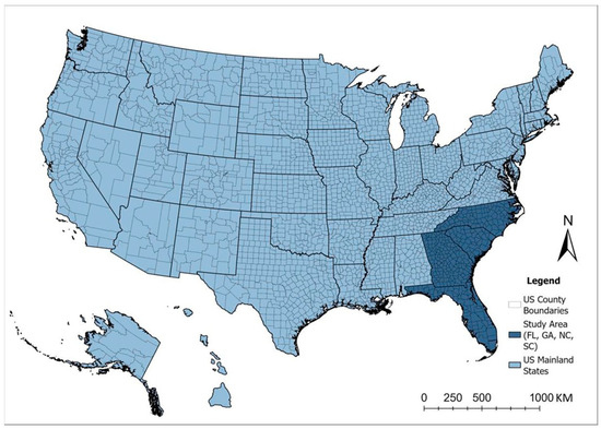
Figure 1.
Study area in the southeastern United States. The map highlights Florida, Georgia, South Carolina, and North Carolina within U.S. county boundaries, representing the study region exposed to recurrent flooding and urbanization pressures.
The unit of spatial analysis is the county, ensuring temporal and spatial consistency across datasets. The study period spans from 2000 to 2019, divided into four 5-year intervals: 2000–2004, 2005–2009, 2010–2014, and 2015–2019.
2.2. Data Collection and Processing
2.2.1. Land Cover Data: National Land Cover Database (NLCD)
Land cover data were obtained from the National Land Cover Database (NLCD), published by the U.S. Geological Survey (USGS). The NLCD provides 30-m resolution raster data at approximately 5-year intervals (2001, 2006, 2011, and 2016), and is widely regarded as the gold standard for longitudinal land use and land cover change (LUCC) analysis in the United States due to its consistent classification methodology, comprehensive spatial coverage, and regular update schedule. For this study, we utilized the products from 2001, 2006, 2011, and 2016, which align closely with our four 5-year study periods (2000–2004, 2005–2009, 2010–2014, and 2015–2019).
“Urban green space” was defined by aggregating seven NLCD classes with ecological or recreational functions: Class 21 (Developed, Open Space), Class 41 (Deciduous Forest), Class 42 (Evergreen Forest), Class 43 (Mixed Forest), Class 52 (Shrub/Scrub), Class 90 (Woody Wetlands), and Class 95 (Emergent Herbaceous Wetlands). These categories were selected because they represent vegetated or semi-natural land covers that provide ecological services (e.g., flood mitigation, habitat provision, microclimate regulation) or recreational value, making them most relevant to the study’s focus on resilience and human–environment interactions.
2.2.2. Flood Hazard Data: FEMA Disaster Declarations
Flood frequency data were obtained from the Federal Emergency Management Agency (FEMA) Disaster Declarations Summaries for U.S. States and Counties, which provides official records of federally declared disasters across the United States. This database is widely recognized as a reliable source for historical disaster information, covering events from 1953 to the present [40].
For this study, disaster events were filtered to include categories directly relevant to flood hazards, namely “Flood,” “Severe Storm,” and “Tropical Storm”, as these event types are most closely associated with inland and coastal flooding processes in the southeastern United States. Events unrelated to flooding, such as wildfires or earthquakes, were excluded to maintain analytical precision.
To capture temporal dynamics, the dataset was aggregated at the county level, which ensures spatial consistency with other socioeconomic and land-use variables. The total number of qualifying flood-related disaster declarations was counted for each county and then summarized for each 5-year interval (2000–2004, 2005–2009, 2010–2014, and 2015–2019). This approach enabled the construction of a flood frequency variable that reflects the intensity of recurrent flooding exposure at the local scale.
However, it is important to note that FEMA disaster declarations reflect officially recognized events, which are influenced not only by hydrological severity but also by political and administrative processes. As a result, some flood events—particularly smaller or recurrent local floods. Although we explored alternative data sources such as remote-sensing-derived flood inundation maps and river streamflow records, these datasets often lack the temporal depth or consistent spatial coverage required for a multi-decade, multi-state analysis. For a longitudinal study spanning hundreds of counties across four southeastern states, the FEMA Disaster Declarations dataset remains advantageous in terms of consistency, nationwide coverage, and official verification. Accordingly, it has been widely adopted in large-scale flood risk and socio-environmental analyses [41,42]. Although the FEMA dataset does not capture the full hydrological frequency of all flood events, it effectively represents major, high-impact flooding occurrences. These severe events themselves constitute critical stressors to urban ecosystems. By their nature, they are capable of causing widespread damage, triggering substantial post-disaster investment, and reshaping long-term land-use planning. Therefore, analyses based on such events provide a valid and essential perspective for understanding how urban green spaces respond to significant, officially recognized disasters. The use of FEMA disaster declarations as a proxy for flood hazard offers several advantages. First, it accounts for both inland and coastal flood events, thereby capturing the multiple hydrological pathways through which floods impact urban and peri-urban green space. Second, the declaration process involves federal and state-level assessment, ensuring consistency and reliability in reporting. Third, aggregating disaster counts across standardized 5-year intervals reduces year-to-year volatility and highlights longer-term trends in flood occurrence.
2.2.3. Population and Income Data: IPUMS NHGIS
County-level demographic and socioeconomic data were obtained from the IPUMS National Historical Geographic Information System (NHGIS), a well-established database that harmonizes decennial U.S. Census and American Community Survey (ACS) estimates across space and time. This integration ensures consistency in geographic boundaries and variable definitions, enhancing comparability across multiple periods. Specifically, we extracted total population and median household income for four intervals—2000, 2005–2009, 2010–2014, and 2015–2019 to correspond with the 5-year green space change analysis. Population density was computed as the ratio of total population to county land area (derived from NLCD data, in hectares).
The NHGIS database is widely used in urban and environmental studies because it provides standardized, long-term, and spatially detailed records of U.S. demographic and socioeconomic conditions. By employing both population density and income measures, the analysis captures critical dimensions of urbanization: demographic pressure on land resources and socioeconomic capacity to adapt to flood risk and green space change. These variables not only reflect baseline human-environment interactions but also allow for cross-county comparisons under varying levels of development and vulnerability.
2.2.4. Annual Development Intensity Data: U.S. Census Bureau and NLCD
County-level records of newly approved housing construction were obtained from the U.S. Census Bureau, one of the most authoritative and comprehensive sources of demographic and housing data in the United States. These data provide annual counts of newly authorized residential housing units, which serve as a robust indicator of development pressure at the county scale. To account for differences in land area across counties, these housing construction counts were standardized using county area (in hectares) derived from the National Land Cover Database (NLCD). This integration enabled the calculation of Annual Development Intensity, expressed as the number of new housing units per hectare per year. By combining Census Bureau housing statistics with NLCD land cover data, this indicator reflects both the scale and spatial distribution of urban expansion, offering a reliable measure of development pressure that is comparable across counties and over time.
2.2.5. Urban Boundary Data: Global Urban Boundaries (GUB) Dataset
Urban boundaries were derived from the Global Urban Boundaries (GUB) dataset, constructed using the 30 m Global Artificial Impervious Area (GAIA) data [40]. The dataset was generated through an automated framework integrating kernel density estimation, cellular automata–based modeling, and morphological refinement, ensuring accurate delineation of urban extents worldwide. Implemented on the Google Earth Engine (GEE) platform, the methodology achieved high reliability, with strong agreement against nighttime light data, high-resolution imagery, and human interpretation.
The GUB dataset provides multi-temporal urban boundaries for seven benchmark years (1990–2018), covering over 65,000 cities larger than 1 km2 at 30 m resolution. Validation results confirmed its robustness in representing both global and regional urban growth, with impervious surface proportions increasing from 53% to 60% over three decades, indicating compact urban expansion.
Given its fine resolution, temporal depth, and rigorous validation, the GUB dataset is recognized as a reliable source for urbanization research and provides a consistent spatial boundary framework for assessing land-use change, ecological processes, and climate-related risks.
Urban Green Space Change Rate (G): Using ArcGIS Pro 3.0 (Esri, Redlands, CA, USA), the above seven land cover types were clipped by the urban boundary and aggregated for each year. County-level green space areas were calculated (in hectares), and the 5-year green space change rate was computed as:
where
- G = Urban green space change rate from year n to n + 5 (%)
- = Green space area in year n
2.3. Generalized Additive Model (GAM)
To explore the distributional patterns of green space change—both increases and decreases—across successive five-year intervals, GAM was employed. GAM is particularly well-suited for this analysis as they allow for flexible modeling of nonlinear and non-monotonic relationships between green space dynamics and multiple predictors, including flood frequency, population density, income, and development intensity. By applying smooth functions to each explanatory variable, the models can capture complex threshold effects and nonlinear trends that traditional linear approaches might overlook, thereby providing a more nuanced understanding of the socio-environmental drivers of green space change. The dependent variable was the 5-year green space change rate per county for the periods: 2000–2004, 2005–2009, 2010–2014, and 2015–2019. Predictors included: Flood Frequency, Annual Development Intensity, Population Density, Median Household Income. Both Time Fixed Effects (to control for differences across periods) and State Fixed Effects (to control for structural variations across states) were included.
Model specification:
where
- = five-year greenspace change rate in county i and period t;
- = intercept;
- = number of FEMA-declared flood events;
- = smooth spline terms for income;
- = smooth spline terms for population density;
- = smooth spline terms for development intensity;
- = state fixed effects;
- = time fixed effects;
- = model residual.
Models were fitted in R using the mgcv package, with smooth terms , and capturing the non-linear effects of continuous predictors. The variables used in the model are summarized in Table 1.

Table 1.
Variables used in the Generalized Additive Model (GAM).
2.4. Logistic Regression Model
To predict the probability of green space degradation or persistence over the 20-year study period, a logistic regression model was constructed. This approach enables the classification of counties into categories of significant urban green space loss versus relative stability or growth, thereby providing insights into the underlying drivers of long-term degradation. By linking degradation outcomes to socio-economic, demographic, and environmental predictors—such as flood frequency, development intensity, and income levels—the model facilitates the identification of high-risk regions. The results can further inform evidence-based policy interventions, such as targeted flood adaptation strategies, land-use regulations, and green infrastructure planning, aimed at mitigating degradation risks and enhancing urban ecological resilience. The dependent variable was ChangeType: 1 = counties experiencing urban green space loss in at least 3 of the 4 time periods, 0 = all other counties. This threshold was designed to capture persistent, long-term degradation rather than short-term fluctuations, identifying counties where urban green space loss occurred consistently across most intervals.
Independent variables included: Total flood events over 20 years, Annual development intensity, Population density, Median household income, Initial green space area (in 2000), State fixed effects were added to control for regional structural differences.
Model specification:
where
- = 1 if greenspace declined in ≥3 periods, else 0;
- = intercept;
- = total FEMA-declared flood events (2000–2019);
- = annual development intensity (new housing units/ha/year);
- = median household income;
- = population density (people/ha);
- = initial greenspace area in 2000;
- = state fixed effects;
- = interaction term;
Equations (2) and (3) represent two complementary analytical relationships capturing short-term and long-term green space dynamics. Equation (2) employs a Generalized Additive Model to analyze the five-year rate of green space change in relation to flood frequency, development intensity, population density, and income, while allowing for nonlinear effects and fixed differences across states and periods. In contrast, Equation (3) applies a logistic regression model to evaluate the 20-year probability that a county experienced long-term green space degradation, incorporating cumulative flood frequency, development pressure, and socioeconomic factors, as well as their interaction. Together, these two models link short-term fluctuations with long-term cumulative outcomes, providing an integrated understanding of how environmental and socioeconomic processes jointly shape urban green space resilience.
An interaction term between flood frequency and income was also added to examine how socioeconomic conditions modify the relationship between flooding and green space degradation. The model was implemented in R 4.5.1 (R Core Team, Vienna, Austria) using the glm() function in R with a logit link, suitable for binary classification problems. The variables used in the logistic regression model are summarized in Table 2.
Table 2.
Variables used in the Logistic Regression Model.
3. Results
To systematically explore patterns and drivers of greenspace change, this study adopted a progressive three-step analytical approach. First, GIS-based spatial analysis was employed to quantify the rate and spatial distribution of greenspace change across southeastern U.S. counties from 2000 to 2019. Second, a Generalized Additive Model was applied to examine non-linear associations between greenspace change and key environmental and socio-economic variables over time. Finally, a logistic regression model was employed to estimate the probability that a county experienced long-term green space degradation as a function of flood frequency, development intensity, and socioeconomic factors [21]. This sequential methodology facilitates a comprehensive investigation, transitioning from spatial description to robust statistical modeling and probabilistic interpretation of greenspace dynamics.
3.1. The Spatial Heterogeneity of Urban Green Space Change
Our spatial analysis reveals that the change in urban green space from 2000 to 2019 was a markedly heterogeneous process across counties in the southeastern United States. Despite a deceleration in the overall rate of loss over time, negative changes dominated large parts of the region, particularly in coastal and low-lying counties prone to recurring flood events. The spatial and temporal variations observed underscore that green space decline is not a uniform process but one shaped by localized environmental and socio-spatial factors.
The temporal trajectory, detailed in Figure 2, underscores a regional shift over the two decades. Between 2000 and 2004, extensive urban green space losses occurred across most of the study area, with numerous counties, particularly in Florida and coastal Georgia, experiencing a decline greater than 10%. During 2005–2009, the extent of severe decline decreased slightly, though a majority of counties continued to experience negative change rates. The subsequent period, 2010–2014, saw a gradual emergence of positive change in certain inland counties of Georgia and North Carolina, indicating partial recovery. By 2015–2019, more counties displayed stable or increasing green space levels, while persistent negative trends remained concentrated in southern Florida and several coastal zones. This temporal trajectory suggests that the most substantial degradation occurred in the early 2000s, followed by a progressive mitigation of these losses in subsequent years.
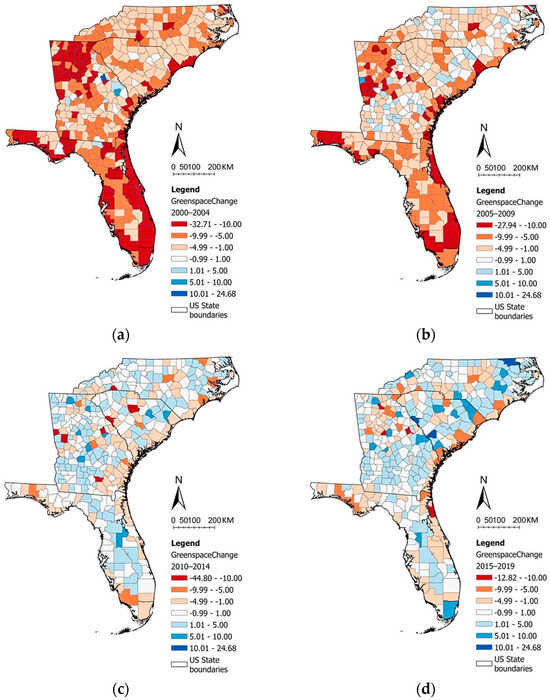
Figure 2.
Spatial distribution of county-level green space change rates in the southeastern United States over four periods: (a) 2000–2004, (b) 2005–2009, (c) 2010–2014, and (d) 2015–2019. The revised color scheme uses a higher-contrast palette to improve visual clarity and distinguish areas of varying change intensity.
To further illustrate the magnitude of these changes, Table 3 summarizes the mean county-level green space area and percentage loss across five-year intervals from 2000 to 2019. The data reveal four consecutive periods of decline: a 9.2% reduction between 2000–2004, followed by a 5.4% decline during 2005–2009, a 0.5% decrease in 2010–2014, and a 1.2% decrease in 2015–2019. Overall, county-level green space area fell from 7322 ha in 2000 to 6188 ha in 2019, representing a cumulative 15.5% loss over two decades. These results confirm that the observed trend reflects a substantial long-term transformation in urban green space coverage rather than short-term statistical variation.
Table 3.
Changes in mean county-level green space area (ha) and percentage loss across five-year periods (2000–2019).
As shown in Figure 3, the classification of counties into seven change-level categories further illustrates these dynamics. In the first period (2000–2004), 88 counties experienced severe degradation (≤−10%), whereas only a negligible number exhibited significant recovery (≥+5%). Over the two decades, the proportion of severely affected counties decreased steadily, falling to 12 counties in the final period, while the share of counties demonstrating notable recovery increased markedly. These results point to a long-term shift in regional patterns of green space change rates, transitioning from widespread degradation toward more stable or improving conditions.
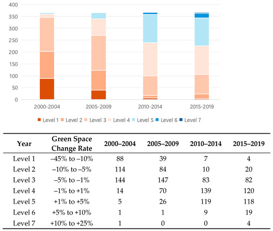
Figure 3.
Number of counties within each green space change rate level (Levels 1–7) for four consecutive periods (2000–2019).
However, Figure 4 reveals that the interplay between long-term change and flooding frequency indicates that this transition is spatially contingent. Counties exposed to high-frequency flood events (≥5 over 20 years) disproportionately experienced persistent negative green space change rates. Of these flood-prone counties, more than one-third of these counties recorded cumulative losses exceeding 5%, whereas only a small proportion achieved stable or positive change over the same period. In contrast, counties with fewer flood disturbances were more likely to maintain or regain green space, highlighting the role of recurrent flooding as a reinforcing factor in long-term degradation patterns.
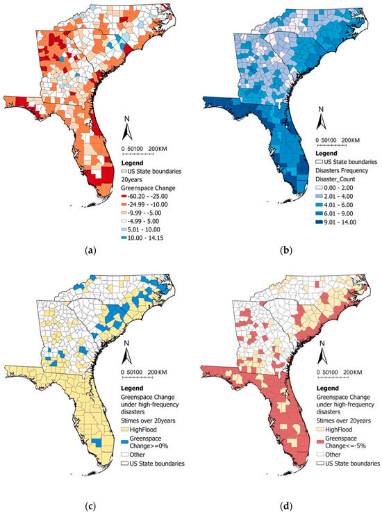
Figure 4.
Spatial distribution of long-term green space change and high-frequency flood exposure in the southeastern United States: (a) cumulative green space change from 2000 to 2019; (b) flood disaster frequency over 20 years; (c) counties with high-frequency floods showing stable or positive green space change (≥0%); (d) counties with high-frequency floods showing significant urban green space loss (≤−5%). The updated palette enhances contrast between positive and negative associations, improving readability of regional variations.
Collectively, these results demonstrate that the rate of urban green space change followed a regional trajectory from widespread, severe losses to partial recovery over the two-decade period. Nonetheless, spatial disparities remained pronounced, and high-frequency flooding emerged as a key driver of sustained green space decline. These findings emphasize the importance of considering both temporal evolution and environmental disturbances in understanding the spatial heterogeneity of green space change rates.
3.2. Modeling the Drivers of Green Space Change: GAM Results
Building upon the spatial analysis presented in the first part, which revealed notable variations in greenspace change across counties with differing flood exposure, this section further investigates the underlying factors driving these patterns using a Generalized Additive Model. By incorporating both environmental and socioeconomic variables, the model allows for a more nuanced understanding of how flood frequency, development intensity, population, and income levels collectively shape long-term greenspace dynamics in the southeastern United States. The coefficient estimates of the GAM are summarized in Table 4.
Table 4.
Coefficient estimates from the Generalized Additive Model (GAM) for factors influencing green space change.
Among the statistically significant factors, flood frequency is a significant and negative linear predictor of the green space change rate (p < 0.01). This coefficient indicates that for each additional presidentially declared flood event, a county’s 5-year green space change rate is expected to decrease by 0.36 percentage points, controlling for other factors.
The non-linear smooth terms revealed more complex relationships. The non-linear effects of socioeconomic variables are presented in Table 5. Annual development intensity (new building rate) emerged as the most powerful predictor, exhibiting a highly significant non-linear effect (p < 0.001). The smooth function revealed a three-phase relationship: The effect of development intensity on greenspace change is distinctly non-linear. An initial, steep decline is observed as development intensity increases to approximately 40, where the rate of loss accelerates sharply. This trend reaches a point of maximum greenspace loss (approximately −13%) at an intensity range of 40–60 units/ha/year. Beyond this range, the rate of loss appears to slightly ease, suggesting a modest rebound; however, this pattern should be interpreted with caution due to the wide confidence intervals and the limited number of observations at very high intensity levels. To improve interpretability, Figure 5 explicitly visualizes the 95% confidence intervals of the fitted GAM curve, which become notably wider at higher development intensity levels, reflecting increasing model uncertainty. By contrast, median income (p = 0.74) and population density (p = 0.09) were not statistically significant predictors. These findings suggest that after accounting for development pressure and flood exposure, socioeconomic indicators such as income and density exert relatively limited influence on green space trajectories.
Table 5.
Results of the Generalized Additive Model for socioeconomic variables affecting green space change.
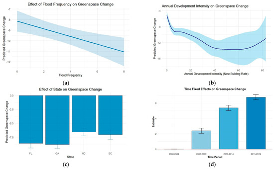
Figure 5.
Effects of key factors on green space change rate from the GAM: (a) Flood frequency (negative trend); (b) Annual development intensity shows a significant nonlinear relationship with green space change. Urban green space loss accelerates rapidly at low levels of development and reaches its maximum (approximately −13%) at an intensity range of 40–60 units/ha/year. Beyond this range, the rate of loss appears to slightly ease, suggesting a modest rebound; however, this trend should be interpreted with caution due to the wide confidence intervals and the small number of observations at very high intensity levels. Shaded area represents the 95% confidence interval of the fitted GAM curve, highlighting wider uncertainty at higher levels of development intensity.; (c) State variations; (d) Time fixed effects showing a progressive recovery over time relative to the 2000–2004 baseline.
State and time fixed effects were also highly significant. Compared to Florida (the reference state), counties in North Carolina and South Carolina demonstrated significantly more positive green space trajectories, with North Carolina exhibiting an average increase of 2.02% (p < 0.01) and South Carolina 1.57% (p < 0.01). In contrast, the difference between Georgia and Florida was not statistically significant (p = 0.55).
Temporal fixed effects showed a progressive trend of green space recovery across the study period. Relative to the 2000–2004 baseline, subsequent periods displayed increasingly positive green space change: +2.39% during 2005–2009, +5.38% during 2010–2014, and +6.75% during 2015–2019 (all p < 0.01).
Overall, the GAM results confirm that higher flood frequency significantly associated with accelerated greenspace loss, while development intensity is the dominant non-linear driver of change. In contrast, income and population density show weaker or insignificant effects. These findings highlight the combined influence of hydrological stressors and human development pressures on greenspace resilience, complementing the spatial patterns observed in the first part of the analysis.
The overall model performance was satisfactory, with an adjusted R2 of 0.46 and deviance explained of 46.4%, indicating that the model captured the main drivers of green space dynamics across the study region.
3.3. Determinants of Long-Term Green Space Degradation: Logistic Regression Results
Finally, we used a logistic regression model to identify the factors that increase the F of a county experiencing long-term (20-year) green space degradation. The results are presented in Table 6.
Table 6.
Logistic regression results on factors influencing long-term greenspace degradation (20-year period).
The model reveals that flood exposure is a key correlate of long-term greenspace decline. Counties experiencing extreme flood frequency (≥10 events) showed a significantly higher probability of greenspace loss over the 20-year period (p = 0.008). A notable interaction effect was observed between moderate flood frequency (6–9 events) and median income, where higher income was paradoxically associated with an increased odds of degradation (OR = 5.84 for the interaction term, p = 0.005). Conversely, in the most flood-prone counties (≥10 events), higher median income was associated with reduced odds of degradation (OR = 0.155, p = 0.030), suggesting a complex interplay between flooding intensity and socioeconomic capacity.
Other variables, including annual development intensity (p = 0.336) and population density (p = 0.943), did not exhibit statistically significant associations with greenspace change. State-level differences were also statistically insignificant, with Georgia (p = 0.096) and South Carolina (p = 0.097) showing only weak associations with higher greenspace loss compared to Florida.
3.4. VIF Analysis
The Variance Inflation Factor (VIF) results indicate that multicollinearity is not a major concern in the logistic regression model. All variables present VIF values well below the conventional threshold of 10, suggesting that the predictors are not excessively correlated. Among them, annual development intensity (VIF = 3.95) and population density (VIF = 3.20) show the highest values, implying a moderate degree of collinearity but remaining within acceptable limits. Flood frequency (VIF = 1.20), median household income (VIF = 1.57), and state fixed effects (VIF = 1.21) exhibit very low multicollinearity, confirming that these variables contribute independent explanatory power to the model. The results of VIF analysis (Table 7) indicate that all predictors show acceptable levels of collinearity.
Table 7.
Variance Inflation Factor (VIF) values for predictor variables, indicating no severe multicollinearity among the independent variables.
These findings emphasize that recurrent flooding exerts the strongest influence on long-term greenspace outcomes, while socioeconomic conditions alone do not significantly alter the trajectory of change unless interacting with flood exposure.
4. Discussion
Our findings reveal that the long-term resilience of urban green space is co-shaped by the persistent hydrological pressure of recurrent flooding and the complex dynamics of urban development, with socio-economic factors acting as a critical mediator.
4.1. The Role of Flooding
The results consistently identify flood frequency as a critical negative correlate of greenspace decline. GIS spatial analysis first revealed a clear clustering effect, with persistent greenspace loss concentrated in flood-prone coastal counties, suggesting a strong spatial coupling between recurrent flooding and greenspace reduction. The GAM model quantified this relationship, showing that each additional flood event was associated with an average decrease of 0.36 percentage points in the five-year greenspace change rate, underscoring the cumulative erosive effect of flooding. Finally, the logistic regression model confirmed this trend over longer time horizons: counties experiencing ten or more flood events were over 18 times more likely to undergo long-term greenspace degradation compared with less exposed areas. The mechanisms through which flooding is associated with greenspace degradation can be understood in both direct and indirect terms. In coastal areas especially, saltwater intrusion and cumulative soil loss often lead to large-scale vegetation decline that is difficult to reverse [43]. Post-disaster recovery and reconstruction efforts tend to prioritize grey infrastructure—such as reinforced seawalls and hard-engineered drainage systems—over ecological restoration [44]. This imbalance not only delays the natural recovery of greenspace but may also encroach upon potential green land. In addition, post-disaster land-use changes or government acquisitions can result in the conversion of greenspace into built-up areas, reinforcing long-term degradation trends [45].
Overall, these patterns highlight that flooding does not directly “cause” urban green space loss but rather operates as a chronic environmental stressor that interacts with urban development pressures and post-disaster land-use dynamics. This interpretation aligns with the reciprocal relationship between land cover change and flood risk, in which urbanization and deforestation amplify flood exposure, while repeated inundation in turn weakens the ecological recovery capacity of urban green spaces.
4.2. The Complex Effects of Urbanization Intensity and Socio-Economic Interactions on Greenspace Change
Beyond flooding, urban development and socioeconomic dynamics also play a critical role in shaping long-term greenspace change. The GAM analysis revealed that annual development intensity exerts a distinctly nonlinear influence on greenspace dynamics, which can be divided into three phases. At low levels of development intensity, even modest increments in new construction were associated with rapid greenspace decline. During this stage, urban growth may rely more on densification and vertical expansion. This process reduces the marginal pressure on the remaining greenspace. [46]. Finally, at very high intensities (>70 units/ha/year), the model suggested a potential rebound or weakening of the marginal effect of development on greenspace loss, albeit with considerable uncertainty. This may be linked to brownfield redevelopment [47], increased reliance on three-dimensional land use, or regulatory requirements for green coverage in high-density zones [48], but could also reflect the limited distribution of extreme-intensity cases in the dataset. Overall, this phased pattern highlights the nonlinear and context-dependent relationship between development intensity and greenspace change, shaped by land availability, modes of urban expansion, and the balance between new conversion and redevelopment.
Beyond development intensity, the logistic regression results revealed a key interaction between flood exposure and income levels in driving long-term greenspace outcomes. A striking finding is that in counties with moderate flood exposure, higher household income was associated with an increased probability of greenspace loss (OR = 5.84). In contrast, in counties facing the most frequent flood exposure, income exhibited a protective effect (OR = 0.155). Such pathways create opportunities for ecological regeneration and the recovery of greenspace buffering functions. Taken together, these contrasting patterns underscore the dual role of income: it can act as both a driver of greenspace degradation and a resource for resilience, depending on the severity of flood risk and the adaptive strategies employed.
This counterintuitive pattern in moderately flood-prone areas can also be explained by the “rebuild and fortify” cycle often observed in wealthier communities. After flood events that cause manageable levels of damage, high-income households and local governments typically have the financial capacity to rebuild quickly, often replacing damaged green areas with more resilient—but less permeable—grey infrastructure such as concrete floodwalls, elevated roads, or expanded residential footprints. These reconstruction efforts, while reducing short-term exposure, can unintentionally displace vegetation and reduce the proportion of permeable land. Moreover, higher property values and redevelopment incentives in these locations may encourage land conversion from ecological or open areas into larger private lots, parking facilities, or housing expansions, further accelerating urban green space loss. This dynamic contrasts with the most flood-prone areas, where extreme exposure prompts more cautious planning, investment in green infrastructure, or retreat strategies, leading to a relative preservation or recovery of vegetated land.
This pattern can be interpreted through three complementary mechanisms. First, under moderate flood exposure, higher-income communities often experience intensified urban development pressure driven by land market dynamics. Attractive locations with manageable flood risks may stimulate real estate investment and land conversion, accelerating urban green space loss. Second, under extreme flood exposure, income translates into greater adaptive capacity. Wealthier jurisdictions have stronger fiscal resources, governance capacity, and institutional flexibility to invest in green infrastructure, flood control, and ecological restoration, thereby mitigating cumulative degradation. Third, political prioritization further reinforces this divergence. High-income areas tend to receive more policy attention and infrastructure funding, leading to faster recovery and proactive resilience planning after major disasters. In contrast, low-income areas facing frequent flooding often suffer from underinvestment and deferred maintenance, resulting in long-term ecological deterioration. Together, these mechanisms highlight that income operates as a context-dependent factor: it may amplify ecological pressure through market-driven urbanization in low-risk contexts, yet enhance resilience through institutional and financial buffering in high-risk environments.
4.3. Integrating Short-Term Dynamics and Long-Term Vulnerability: A Complementary Interpretation of Two Models
The two approaches are complementary, reflecting the distinction between short-term dynamics and long-term cumulative effects. The GAM captures short-term fluctuations, whereas the logistic regression highlights 20-year cumulative outcomes. This contrast is evident in the results. In the short-term model, development intensity emerged as the strongest predictor, shaping the immediate rate of greenspace loss. By contrast, the interaction between flooding and income became significant only over the long term. This finding suggests that socio-economic responses to environmental hazards unfold gradually over time. Their cumulative effects ultimately determine regional resilience or vulnerability.
Although income and population density showed weak or insignificant effects in the short-term GAM model, income demonstrated a significant interaction effect in the long-term logistic regression. This apparent contrast does not indicate inconsistency but rather highlights the different temporal scales at which socio-economic factors operate. The GAM captures short-term (five-year) fluctuations in greenspace change rates, where immediate physical drivers—such as flooding and development intensity—dominate. In such short windows, community income cannot prevent trees from being uprooted or parks from being inundated; responses are chaotic and driven primarily by the hazard itself. Consequently, the direct statistical effect of income during these intervals remains weak.
Over two decades, however, the cumulative outcomes are shaped by adaptive capacity and strategic decision-making processes that are fundamentally linked to economic resources. Wealthier counties may be able to recover more rapidly, invest in flood-resilient infrastructure, and restore or expand green spaces, whereas disadvantaged areas experience repeated degradation and deferred recovery. The significant interaction between income and flood exposure suggests that income is not a direct driver of greenspace loss. Instead, it moderates the recovery pathways activated under chronic hazard exposure. In this sense, the contrast between the two models underscores that socio-economic responses to environmental stress require time to manifest, and their cumulative consequences ultimately shape regional resilience or vulnerability. Overall, the differentiated findings of the two models underscore the importance of integrating short-term dynamics with long-term trends. While the short-term perspective reveals immediate mechanisms of change, the long-term analysis reflects structural outcomes shaped by the interaction of institutional, economic, and environmental forces.
Nevertheless, future climate projections indicate intensified rainfall, rising sea levels, and more frequent extreme precipitation. These trends may reverse the recovery observed since the early 2000s. Without continued adaptation and investment in resilient green infrastructure, these accelerating climatic pressures could undermine long-term urban ecological resilience, particularly in low-lying and coastal counties. This highlights the need for proactive climate adaptation policies that anticipate future hydrological risks rather than solely responding to past patterns.
4.4. Limitations and Future Directions
First, the modifiable areal unit problem (MAUP) remains a challenge. The county scale is an effective unit for regional analysis, yet it inevitably masks substantial intra-county heterogeneity. Green space change and flood impacts are often highly localized, and aggregate measures may overlook neighborhood-level disparities. For example, neighborhood-scale flood loss studies have demonstrated that finer spatial units can reveal substantial heterogeneity that is masked at aggregated levels. A comparative analysis of FEMA’s Hazus, FAST, and HEC-FIA models across census blocks in Jefferson Parish, Louisiana, found that building-level loss estimates varied significantly depending on local characteristics such as foundation type, elevation, and replacement cost. Similarly, in our study context, a county-level summary might show stable or slightly increasing green space overall, while concealing critical environmental inequities within the county. Urban Green space loss may be highly concentrated in low-income, flood-prone riverfront communities—where post-disaster reconstruction often prioritizes grey infrastructure over ecological restoration—whereas increases may occur in wealthier suburban areas through new parks or larger residential lots. In such cases, county averages obscure substantial redistributions of ecological assets that disproportionately disadvantage vulnerable populations. Therefore, our county-level findings serve not only to identify broad regional risk patterns but also as a diagnostic tool to highlight counties that warrant further, fine-scale investigation to uncover these localized environmental justice dynamics. [49]. Future research should incorporate higher-resolution data (e.g., census tracts or block groups) to capture finer-scale dynamics and to address potential issues of environmental justice. Moreover, our county-level design cannot establish a one-directional causal chain between flooding and green-space loss; flood impacts are likely concentrated in coastal and low-lying settings, whereas inland effects may be indirect. Future work should couple tract-level analyses with hydrological data (e.g., streamflow records or remote-sensing-based flood-inundation maps) to disentangle direct biophysical damage from post-disaster redevelopment and land-use transition dynamics.
In addition, the FEMA Disaster Declarations dataset used in this study, while consistent and officially verified, captures only federally declared disasters and may therefore omit smaller or localized flood events. Nevertheless, these major, high-impact floods represent critical stressors that are capable of causing widespread ecological disturbance, triggering substantial reconstruction, and reshaping long-term land-use patterns. Analyses based on such officially recorded events thus provide a valid and policy-relevant perspective for understanding how urban green spaces respond to severe hydrological shocks.
Second, the homogenization of “green space” may obscure important functional differences. In this study, green space was treated as a single category for analytical consistency. However, a manicured urban park, a private yard, and a natural wetland or woodland provide markedly different ecological and social functions. This generalization, while necessary to ensure temporal and spatial comparability across datasets, inevitably conceals the ecological and social diversity among different types of green spaces. For instance, forests and wetlands play key roles in hydrological regulation and biodiversity maintenance, whereas parks and open spaces primarily contribute to recreation and community well-being. Treating them as a unified class may therefore obscure how particular types respond differently to flood exposure or urban development pressures. Consequently, the interpretation of our findings should be understood as reflecting overall regional trends rather than type-specific dynamics. Future research should differentiate green space types (e.g., public parks, private gardens, urban forests, wetlands) to better understand their heterogeneous vulnerabilities and capacities vary across different contexts.
Moreover, differences in accessibility—particularly between public and private green spaces—represent another important dimension of inequality. While public parks and community green areas provide open access and collective benefits, private gardens and enclosed green spaces primarily serve restricted user groups. This accessibility divide has implications for environmental justice, as lower-income populations may have less access to high-quality green space even when total green area appears sufficient at the aggregate level. Future studies should therefore integrate social accessibility indicators to better capture equity-related aspects of green space resilience.
Third, the causal mechanisms behind observed patterns remain underexplored. While the results demonstrate strong associations between development intensity and urban green space loss, it is unclear whether higher development intensity directly drives green space reduction, or whether both are shaped by broader policy or economic drivers [50].
The findings underscore the need to integrate urban planning with disaster risk reduction, particularly in flood-prone areas. Stricter land-use regulations and the adoption of nature-based solutions and green infrastructure can simultaneously reduce flood risk and enhance community well-being. Future work should simulate the effectiveness of such policies under different climate and development scenarios to provide robust evidence for long-term resilience planning [51].
5. Conclusions
This study developed an integrated multi-stage framework combining GIS-based spatial analysis, Generalized Additive Model, and logistic regression to examine urban greenspace change across southeastern U.S. counties from 2000 to 2019. The findings reveal a complex trajectory characterized by an initial phase of widespread decline followed by uneven and localized recovery, highlighting the interplay of environmental stressors, urban development intensity, and socio-economic capacity.
Recurrent flooding consistently emerged as a dominant correlate of greenspace vulnerability, underscoring the cumulative erosive effects of repeated hydrological disturbances on urban ecosystems. Urban development shaped greenspace change in nonlinear and context-dependent ways, reflecting the complex role of growth and redevelopment. Socio-economic conditions further influenced resilience, acting both as pressures that can accelerate loss and as resources that enable protection under severe hazard exposure.
Overall, this study demonstrates that greenspace vulnerability in flood-prone regions is shaped not by single factors but by the interaction of hydrological stress, urban development dynamics, and socio-economic capacity. Policy efforts should prioritize stricter land-use regulation, investment in nature-based solutions, and climate-adaptive planning in flood-prone areas. The analytical framework and findings presented here provide transferable insights for advancing ecological resilience and sustainable urban growth in flood-affected regions worldwide. Similar strategies have been successfully implemented in several international contexts, demonstrating the broader applicability of these approaches. For example, the city of Ghent (Belgium) has integrated green–blue networks and adaptive zoning to manage flood risks while enhancing urban biodiversity, providing a European model for nature-based flood resilience [24]. Likewise, Zhengzhou (China) has promoted the “Sponge City” initiative, combining permeable surfaces, wetland restoration, and green corridors to mitigate urban flooding and improve ecological connectivity [29]. These examples highlight that effective integration of land-use regulation with nature-based planning can generate co-benefits for flood management, ecological restoration, and social well-being, offering transferable insights for flood-prone regions worldwide. Future research could further integrate nonlinear machine learning approaches, such as kernel extreme learning machines (K-ELM), to enhance the spatio-temporal prediction of LUCC–flood interactions and capture complex socio-ecological feedbacks [52,53].
Author Contributions
Conceptualization, K.Z. and X.M.; methodology, K.Z. and X.M.; software, K.Z.; validation, X.M.; formal analysis, K.Z.; investigation, K.Z.; resources, K.Z.; data curation, K.Z.; writing—original draft preparation, K.Z.; writing—review and editing, X.M.; visualization, K.Z.; supervision, X.M. All authors have read and agreed to the published version of the manuscript.
Funding
This research received no external funding.
Data Availability Statement
The original contributions presented in this study are included in the article. Further inquiries can be directed to the corresponding author.
Conflicts of Interest
The authors declare no conflicts of interest.
References
- Lepczyk, C.A.; Aronson, M.F.J.; Evans, K.L.; Goddard, M.A.; Lerman, S.B.; MacIvor, J.S. Biodiversity in the City: Fundamental Questions for Understanding the Ecology of Urban Green Spaces for Biodiversity Conservation. BioScience 2017, 67, 799–807. [Google Scholar] [CrossRef]
- Heo, S.; Bell, M.L. Investigation on Urban Greenspace in Relation to Sociodemographic Factors and Health Inequity Based on Different Greenspace Metrics in 3 US Urban Communities. J. Expo. Sci. Environ. Epidemiol. 2023, 33, 218–228. [Google Scholar] [CrossRef] [PubMed]
- Hunter, R.F.; Cleland, C.; Cleary, A.; Droomers, M.; Wheeler, B.W.; Sinnett, D.; Nieuwenhuijsen, M.J.; Braubach, M. Environmental, Health, Wellbeing, Social and Equity Effects of Urban Green Space Interventions: A Meta-Narrative Evidence Synthesis. Environ. Int. 2019, 130, 104923. [Google Scholar] [CrossRef]
- Sugiyama, T.; Villanueva, K.; Knuiman, M.; Francis, J.; Foster, S.; Wood, L.; Giles-Corti, B. Can Neighborhood Green Space Mitigate Health Inequalities? A Study of Socio-Economic Status and Mental Health. Health Place 2016, 38, 16–21. [Google Scholar] [CrossRef]
- Trenberth, K.E.; Dai, A.; Rasmussen, R.M.; Parsons, D.B. The Changing Character of Precipitation. Bull. Am. Meteorol. Soc. 2003, 84, 1205–1218. [Google Scholar] [CrossRef]
- Gudmundsson, L.; Boulange, J.; Do, H.X.; Gosling, S.N.; Grillakis, M.G.; Koutroulis, A.G.; Leonard, M.; Liu, J.; Müller Schmied, H.; Papadimitriou, L.; et al. Globally Observed Trends in Mean and Extreme River Flow Attributed to Climate Change. Science 2021, 371, 1159–1162. [Google Scholar] [CrossRef] [PubMed]
- Zhou, S.; Kwan, C. Cumulative Exposure to Natural Hazards and Mental Health in China: Are Older People More Vulnerable or More Resilient Than Younger and Middle-Aged Adults? Int. J. Disaster Risk Sci. 2024, 15, 277–289. [Google Scholar] [CrossRef]
- Paulik, R.; Stephens, S.; Wild, A.; Wadhwa, S.; Bell, R.G. Cumulative Building Exposure to Extreme Sea Level Flooding in Coastal Urban Areas. Int. J. Disaster Risk Reduct. 2021, 66, 102612. [Google Scholar] [CrossRef]
- United Nations Department of Economic and Social Affairs. World Urbanization Prospects: The 2014 Revision; United Nations: New York, NY, USA, 2015. [Google Scholar]
- Jia, Y.; Chen, Z.; Lu, X.; Sheng, S.; Huang, J.; Wang, Y. The Degradation and Marginal Effects of Green Space under the Stress of Urban Sprawl in the Metropolitan Area. Urban For. Urban Green. 2024, 95, 128318. [Google Scholar] [CrossRef]
- Volkov, D.L.; Zhang, K.; Johns, W.E.; Willis, J.K.; Hobbs, W.; Goes, M.; Zhang, H.; Menemenlis, D. Atlantic Meridional Overturning Circulation Increases Flood Risk along the United States Southeast Coast. Nat. Commun. 2023, 14, 5095. [Google Scholar] [CrossRef]
- Nagy, R.C.; Lockaby, B.G. Urbanization in the Southeastern United States: Socioeconomic Forces and Ecological Responses along an Urban-Rural Gradient. Urban. Ecosyst. 2011, 14, 71–86. [Google Scholar] [CrossRef]
- Tyler, J.; Entress, R.M.; Sun, P.; Noonan, D.; Sadiq, A. Is Flood Mitigation Funding Distributed Equitably? Evidence from Coastal States in the Southeastern United States. J. Flood Risk Manag. 2023, 16, e12886. [Google Scholar] [CrossRef]
- Osei Owusu, R.; Rigolon, A. What Has Contributed to Green Space Inequities in U.S. Cities? A Narrative Review. J. Plan. Lit. 2025, 40, 59–76. [Google Scholar] [CrossRef]
- Wing, O.E.J.; Lehman, W.; Bates, P.D.; Sampson, C.C.; Quinn, N.; Smith, A.M.; Neal, J.C.; Porter, J.R.; Kousky, C. Inequitable Patterns of US Flood Risk in the Anthropocene. Nat. Clim. Change 2022, 12, 156–162. [Google Scholar] [CrossRef]
- Shahfahad; Rihan, M.; Islam, M.R.; Ansari, I.; Talukdar, S.; Siddiqui, A.M.; Rahman, A. Decadal Pattern of Built-up Expansion and Its Consequences on Urban Green and Blue Space Fragmentation. J. Indian Soc. Remote Sens. 2025, 53, 949–964. [Google Scholar] [CrossRef]
- Lin, B.; Meyers, J.; Barnett, G. Understanding the Potential Loss and Inequities of Green Space Distribution with Urban Densification. Urban For. Urban Green. 2015, 14, 952–958. [Google Scholar] [CrossRef]
- Wu, S.; Wang, D.; Yan, Z.; Wang, X.; Han, J. Spatiotemporal Dynamics of Urban Green Space in Changchun: Changes, Transformations, Landscape Patterns, and Drivers. Ecol. Indic. 2023, 147, 109958. [Google Scholar] [CrossRef]
- Dasallas, L.; Kim, Y.; An, H. Case Study of HEC-RAS 1D–2D Coupling Simulation: 2002 Baeksan Flood Event in Korea. Water 2019, 11, 2048. [Google Scholar] [CrossRef]
- Sarkar, S.; Himesh, S. Assessing the Impact of Modified LULC on Extreme Hydrological Event over a Complex Terrain: A Case Study for Kodagu 2018 Flood Event. J. Atmos. Sol.-Terr. Phys. 2022, 240, 105961. [Google Scholar] [CrossRef]
- Gupta, L.; Dixit, J. Assessment of Urban Flood Susceptibility and Role of Urban Green Space (UGS) on Flooding Susceptibility Using GIS-Based Probabilistic Models. Environ. Monit. Assess. 2023, 195, 1518. [Google Scholar] [CrossRef]
- Saadatkhah, N.; Tehrani, M.H.; Mansor, S.; Khuzaimah, Z.; Kassim, A.; Saadatkhah, R. Impact Assessment of Land Cover Changes on the Runoff Changes on the Extreme Flood Events in the Kelantan River Basin. Arab. J. Geosci. 2016, 9, 687. [Google Scholar] [CrossRef]
- Wang, M.; Zhao, J.; Xiong, Z.; Zhang, M.; Wang, L.; Tan, S.K. Strategic Deployment of Nature-Based Solutions for Urban Flood Management in High-Density Urban Landscapes. Ecol. Indic. 2025, 176, 113681. [Google Scholar] [CrossRef]
- Li, L.; Uyttenhove, P.; Van Eetvelde, V. Planning Green Infrastructure to Mitigate Urban Surface Water Flooding Risk—A Methodology to Identify Priority Areas Applied in the City of Ghent. Landsc. Urban Plan. 2020, 194, 103703. [Google Scholar] [CrossRef]
- Le, T.; Kyle, G.T.; Tran, T. Using Public Participation Gis to Understand Texas Coastal Communities’ Perceptions and Preferences for Urban Green Space Development in Connection to Their Perceptions of Flood Risk. Urban For. Urban Green. 2024, 95, 128330. [Google Scholar] [CrossRef]
- Reu Junqueira, J.; Serrao-Neumann, S.; White, I. Using Green Infrastructure as a Social Equity Approach to Reduce Flood Risks and Address Climate Change Impacts: A Comparison of Performance between Cities and Towns. Cities 2022, 131, 104051. [Google Scholar] [CrossRef]
- Morrison, R.R.; Simonson, K.; McManamay, R.A.; Carver, D. Degradation of Floodplain Integrity within the Contiguous United States. Commun. Earth Environ. 2023, 4, 215. [Google Scholar] [CrossRef]
- Asl, S.R. Green Spaces and Flood Vulnerability in Urbanising Regions: A Case Study in the Philadelphia Metropolitan Area. Environ. Hazards 2024, 1–23. [Google Scholar] [CrossRef]
- Wang, J.; Zhao, M.; Xu, M.; Li, Y.; Gou, A. Effect of Land Cover Types Evolution in Megacities on Flood Regulation Capacity: The Case of Zhengzhou since 1990. Nat. Hazards 2025, 121, 3001–3021. [Google Scholar] [CrossRef]
- Ambily, P.; Chithra, N.R.; Firoz C, M.; Viswanath, S. Ecological Flood Resilience Index (EFRI) to Assess the Urban Pluvial Flood Resilience of Blue-Green Infrastructure: A Case from a Southwestern Coastal City of India. Int. J. Disaster Risk Reduct. 2024, 113, 104867. [Google Scholar] [CrossRef]
- Gupta, L.; Dixit, J. Spatial Analysis of Urban Green Space and Its Utilization Rate for the Flood-Prone Region Assam, India. Environ. Dev. Sustain. 2024, 27, 17493–17523. [Google Scholar] [CrossRef]
- Li, Z.; Wang, Z.; Wu, L.; Huang, W.; Peng, W. Evaluating the Effect of Building Patterns on Urban Flooding Based on a Boosted Regression Tree: A Case Study of Beijing, China. Hydrol. Process. 2023, 37, e14932. [Google Scholar] [CrossRef]
- Luo, K.; Zhang, X. Increasing Urban Flood Risk in China over Recent 40 Years Induced by LUCC. Landsc. Urban Plan. 2022, 219, 104317. [Google Scholar] [CrossRef]
- Kim, H.W.; Kim, J.-H.; Li, W.; Yang, P.; Cao, Y. Exploring the Impact of Green Space Health on Runoff Reduction Using NDVI. Urban For. Urban Green. 2017, 28, 81–87. [Google Scholar] [CrossRef]
- Hu, G.; Zhang, Y.; Chen, C.; Shen, Z.; Hu, Y.; Yin, H.; Shao, Z.; Zheng, H.; Chen, F. Exploring the Decentralized Blue-Green Infrastructure Network Layouts for Urban Flood Risk Management. Landsc. Ecol. Eng. 2025, 21, 1–4. [Google Scholar] [CrossRef]
- Feng, B.; Zhang, Y.; Bourke, R. Urbanization Impacts on Flood Risks Based on Urban Growth Data and Coupled Flood Models. Nat. Hazards 2021, 106, 613–627. [Google Scholar] [CrossRef]
- Muangsri, S.; McWilliam, W.; Lawson, G.; Davies, T. Evaluating Capability of Green Stormwater Infrastructure on Large Properties toward Adaptive Flood Mitigation: The HLCA+C Methodology. Land 2022, 11, 1765. [Google Scholar] [CrossRef]
- Coletta, V.R.; Pagano, A.; Zimmermann, N.; Davies, M.; Butler, A.; Fratino, U.; Giordano, R.; Pluchinotta, I. Socio-Hydrological Modelling Using Participatory System Dynamics Modelling for Enhancing Urban Flood Resilience through Blue-Green Infrastructure. J. Hydrol. 2024, 636, 131248. [Google Scholar] [CrossRef]
- Alves, A.; Vojinovic, Z.; Kapelan, Z.; Sanchez, A.; Gersonius, B. Exploring Trade-Offs among the Multiple Benefits of Green-Blue-Grey Infrastructure for Urban Flood Mitigation. Sci. Total Environ. 2020, 703, 134980. [Google Scholar] [CrossRef]
- Li, X.; Gong, P.; Zhou, Y.; Wang, J.; Bai, Y.; Chen, B.; Hu, T.; Xiao, Y.; Xu, B.; Yang, J.; et al. Mapping Global Urban Boundaries from the Global Artificial Impervious Area (GAIA) Data. Environ. Res. Lett. 2020, 15, 094044. [Google Scholar] [CrossRef]
- Xian, S.; Lin, N.; Hatzikyriakou, A. Storm Surge Damage to Residential Areas: A Quantitative Analysis for Hurricane Sandy in Comparison with FEMA Flood Map. Nat. Hazards 2015, 79, 1867–1888. [Google Scholar] [CrossRef]
- Karamouz, M.; Fereshtehpour, M.; Ahmadvand, F.; Zahmatkesh, Z. Coastal Flood Damage Estimator: An Alternative to FEMA’s HAZUS Platform. J. Irrig. Drain. Eng. 2016, 142, 04016016. [Google Scholar] [CrossRef]
- Barui, I.; Bhakta, S.; Ghosh, K. Storm Surge-Induced Soil Salinization and Its Impact on Agriculture in the Coastal Area of the Indian Sundarban. Environ. Dev. 2025, 56, 101250. [Google Scholar] [CrossRef]
- De Bruijn, K.M.; Maran, C.; Zygnerski, M.; Jurado, J.; Burzel, A.; Jeuken, C.; Obeysekera, J. Flood Resilience of Critical Infrastructure: Approach and Method Applied to Fort Lauderdale, Florida. Water 2019, 11, 517. [Google Scholar] [CrossRef]
- Velilla, E.; Snethlage, J.; Poelman, M.; Van Der Meer, I.M.; Van Der Werf, A.; Deolu-Ajayi, A.O.; Van Belzen, J. Too Salty to Farm: Rethinking Coastal Land Use in Response to Soil Salinization. Restor. Ecol. 2025, 33, e70006. [Google Scholar] [CrossRef]
- Handayani, H.H.; Murayama, Y.; Ranagalage, M.; Liu, F.; Dissanayake, D. Geospatial Analysis of Horizontal and Vertical Urban Expansion Using Multi-Spatial Resolution Data: A Case Study of Surabaya, Indonesia. Remote Sens. 2018, 10, 1599. [Google Scholar] [CrossRef]
- Glumac, B.; Decoville, A. Brownfield Redevelopment Challenges: A Luxembourg Example. J. Urban Plann. Dev. 2020, 146, 05020001. [Google Scholar] [CrossRef]
- Zhou, S.; Nijhuis, S.; Dijkstra, R. Towards a Pattern Language for Green Space Design in High Density Urban Developments. J. Urban Des. 2024, 29, 576–597. [Google Scholar] [CrossRef]
- Mostafiz, R.B.; Friedland, C.J.; Rahman, M.A.; Rohli, R.V.; Tate, E.; Bushra, N.; Taghinezhad, A. Comparison of Neighborhood-Scale, Residential Property Flood-Loss Assessment Methodologies. Front. Environ. Sci. 2021, 9, 734294. [Google Scholar] [CrossRef]
- Blum, A.G.; Ferraro, P.J.; Archfield, S.A.; Ryberg, K.R. Causal Effect of Impervious Cover on Annual Flood Magnitude for the United States. Geophys. Res. Lett. 2020, 47, e2019GL086480. [Google Scholar] [CrossRef]
- Dawson, C. Advancing Blue-Green Infrastructure Design with Synthetic 3D Drainage Channels: A Scenario-Based Flood Model in Nova Scotia, Canada. Nat.-Based Solut. 2025, 7, 100238. [Google Scholar] [CrossRef]
- Lin, Y.; Zhang, T.; Ye, Q.; Cai, J.; Wu, C.; Khirni Syed, A.; Li, J. Long-Term Remote Sensing Monitoring on LUCC around Chaohu Lake with New Information of Algal Bloom and Flood Submerging. Int. J. Appl. Earth Obs. Geoinf. 2021, 102, 102413. [Google Scholar] [CrossRef]
- Zhang, X.; Lin, P.; Chen, H.; Yan, R.; Zhang, J.; Yu, Y.; Liu, E.; Yang, Y.; Zhao, W.; Lv, D.; et al. Understanding Land Use and Cover Change Impacts on Run-off and Sediment Load at Flood Events on the Loess Plateau, China. Hydrol. Process. 2018, 32, 576–589. [Google Scholar] [CrossRef]


Disclaimer/Publisher’s Note: The statements, opinions and data contained in all publications are solely those of the individual author(s) and contributor(s) and not of MDPI and/or the editor(s). MDPI and/or the editor(s) disclaim responsibility for any injury to people or property resulting from any ideas, methods, instructions or products referred to in the content. |
© 2025 by the authors. Licensee MDPI, Basel, Switzerland. This article is an open access article distributed under the terms and conditions of the Creative Commons Attribution (CC BY) license (https://creativecommons.org/licenses/by/4.0/).