Application of Classical and Quantum-Inspired Methods Through Multi-Objective Optimization for Parameter Identification of a Multi-Story Prototype Building

Abstract

This study proposes a new approach to identify structural parameters under seismic excitation using classical and quantum-inspired algorithms. Traditional methods often struggle with complex effects, noise, and computing limits. A five-story building model with mass–spring–damper system was tested to find properties during earthquakes. The study used optimization methods including Genetic Algorithm (GA), Particle Swarm Optimization (PSO), and five quantum-inspired versions: Quantum Genetic Algorithm (QGA), Quantum Particle Swarm Optimization (QPSO), Quantum Non-Dominated Sorting Genetic Algorithm II (QNSGA-II), Quantum Differential Evolution (QDE), and Quantum Simulated Annealing (QSA). Additionally, statistical analysis used Shapiro–Wilk for normality, Levene and Bartlett for variance, ANOVA with Tukey–Bonferroni comparisons, Bootstrap model ranking, and Borda count. The results show that the quantum-inspired methods perform better than classical ones. QSA reduced mean squared error (MSE) by 15.3% compared to GA, and QNSGA-II reduced MSE by 8.6% and root mean squared error (RMSE) by 3.5%, with less variation and tighter rankings. The framework addresses computing cost and response time; quantum methods need significant computing power and their accuracy suits offline earthquake assessments and model updates. This balance helps monitor building health when real-time speed is less critical but accuracy matters. The method provides a scalable tool for checking civil structures and could enable digital twins.

1. Introduction

Numerical modeling represents the dynamic behavior of buildings through assumptions about materials, boundaries, and loads, typically using finite element and modal analysis to estimate vibrations, natural frequencies, and mode shapes. Despite its scalability, it is computationally intensive and may lead to inaccuracies [1]. Wang et al. developed a response-surface–based finite element model–updating technique for a 120 m super high-rise, reducing the error between the measured and simulated natural frequencies to <5% and thereby establishing a reliable benchmark for subsequent damage detection [2]. Identifying structural parameters accurately is critical for ensuring safety, optimizing performance during earthquakes, and enabling effective health monitoring, vibration control, and maintenance.

Hybrid techniques combine methods such as dynamic and ambient vibration testing to refine numerical models, leveraging their respective strengths while introducing added complexity and cost [3]. Accurate modeling and parameter estimation are vital for designing control laws like state feedback and active disturbance rejection control [4,5] and for enabling effective algebraic observers for state estimation [6].

Several approaches have been proposed for parameter identification under seismic excitation. Ji et al. [7] introduced an iterative Least Squares (LS) technique to jointly estimate structural parameters and unknown ground motions, achieving noise robustness. Similarly, ref. [8] presented an adaptive LS-based method for tracking time-varying parameters for damage detection. Concha et al. used adaptive observers with integral filters to estimate damping/mass and stiffness/mass ratios, ensuring positivity via projection techniques [9], while [10] applied modal analysis to estimate natural frequencies.

On the other hand, another approach provides a sophisticated approach that combines wavelet analysis with mode decomposition for improved accuracy in identifying critical structural parameters under dynamic loading conditions.

Optimization-based parametric identification aims to minimize discrepancies between measured and modeled structural responses [11]. Gradient-based algorithms such as Gauss–Newton [12], Levenberg–Marquardt [13,14], and conjugate gradients [15] require derivative calculations. In contrast, heuristic methods like GA [14,16], PSO [14], and simulated annealing are better suited for global, non-convex problems. Bayesian methods, including MCMC [17], offer probabilistic parameter estimation in nonlinear models [18].

Soft computing techniques—fuzzy logic, neural networks, swarm intelligence, and evolutionary computing—support modeling, uncertainty management, and structural reliability evaluation [19]. They have been applied in simulation and optimization tasks, such as topological and shape optimization. Studies comparing NSGA-II and PSO for multi-objective design under seismic loads show both improved performance and reduced weight, with PSO often yielding better results [20]. Soft computing also aids in inverse identification problems and managing uncertainties, using fuzzy logic to model stress–strain behavior [19]. For example, Chisari et al. proposed a GA to calibrate FE models of base-isolated bridges by fitting Young’s modulus and isolator stiffness [21], and Quaranta et al. used DE and PSO to identify Bouc–Wen model parameters of seismic isolators, with DE outperforming PSO [22]. Marano et al. applied a modified GA to large systems, improving performance under noisy data [23]. Károly et al. showed that DE outperformed PSO in estimating parameters of a simplified nonlinear building model, though the model’s simplification limited applicability to complex structures [24]. Salaas et. al. optimized a hybrid vibration-control system that couples base isolation with a tuned liquid column damper (TLCD) using metaheuristic search; for a benchmark tall building they reported up-to-40% drops in peak floor accelerations relative to an isolated-only baseline [25].

Parametric identification of stiffness and damping remains challenging due to modeling and measurement uncertainties. Traditional methods like GA and PSO are moderately complex, but become resource-intensive in multi-objective contexts. In contrast, quantum-inspired algorithms (QGA, QPSO, QNSGA-II, QDE, QSA) exploit superposition to explore solution spaces more effectively. These methods, though computationally demanding, improve convergence and are valuable in structural simulations [26], provided that resource constraints are considered. Lee et al. introduced a quantum-based harmony-search (QbHS) algorithm for simultaneous size and topology optimization of truss structures; on 20-, 24-, and 72-bar trusses the QbHS consistently converged to lighter designs than classical evolutionary methods while respecting frequency and displacement limits [27]. In conclusion, various optimization techniques for parametric identification include deterministic methods like Least Squares Estimation (LSE) and Kalman Filtering, which are robust but noise-sensitive, and heuristic algorithms, such as GA and PSO, which better handle complexity but may face premature convergence issues. Despite the increasing popularity of quantum-inspired metaheuristics in optimization, their application to structural parameter identification remains limited, particularly in civil structures subject to seismic loading. Moreover, while several works have compared classical algorithms like GA and PSO, few have addressed the robustness and reproducibility of results through formal statistical validation frameworks.

This study addresses this gap by proposing a multi-objective optimization approach for the identification of stiffness and damping parameters in a five-story civil structure using both classical and quantum-inspired metaheuristics. The methodology includes a comparative analysis of seven algorithms and incorporates a comprehensive statistical validation process, including tests for normality, variance homogeneity, and ranking consistency. The contribution of this work lies not only in demonstrating the performance of quantum-inspired models such as QNSGA-II and QSA, but also in offering a statistically rigorous and replicable framework for structural parameter estimation, with potential applications in structural health monitoring, vibration control, and seismic engineering. Each method was applied over 30 independent runs using experimental seismic data, and the performance was assessed based on the accuracy of the identified parameters and statistical robustness. Error metrics include MSE, RMSE, MAE, and $R^2$. Normality was assessed with the Shapiro–Wilk test; variance homogeneity was checked using Levene and Bartlett tests. ANOVA with Tukey–Bonferroni post hoc comparisons and Bonferroni-corrected t-tests were used to identify significant inter-model differences while controlling for Type I errors.

The paper is organized as follows: Section 2 introduces the mathematical model and multi-objective function. Section 3 details the optimization methods. Section 4 presents the experimental and statistical results. Section 5 discusses the findings and future works, and Section 6 concludes the work.

2. Parametric Identification

This section introduces the mathematical framework used in the study, focusing on parametric identification to accurately characterize the system’s dynamics.

2.1. Civil Structure Model

Let the approximation of a civil structure in a single axis of motion be modeled in the form according to [28]:

$${\mathbf{M}}_{\mathbf{s}}\ddot{\mathbf{x}}\left(t\right)+{\mathbf{C}}_{\mathbf{s}}\dot{\mathbf{x}}\left(t\right)+{\mathbf{K}}_{\mathbf{s}}\mathbf{x}\left(t\right)=-{\mathbf{M}}_{\mathbf{s}}\mathbf{l}{\ddot{x}}_g\left(t\right),$$

(1)

where ${\ddot{x}}_g\left(t\right)$ is the acceleration of the earth caused by an earthquake that can be measured with accelerometers. Additionally, ${\mathbf{M}}_{\mathbf{s}},{\mathbf{C}}_{\mathbf{s}},{\mathbf{K}}_{\mathbf{s}}\in {\mathbb{R}}^{n\times n}$ represent the matrices of total masses, damping coefficients, and stiffness, respectively; furthermore, $\mathbf{l}$ is a distribution vector of the earthquake on all floors. The mentioned matrices can be defined as

$$\begin{array}{cc}\hfill {\mathbf{M}}_{\mathbf{s}}=& diag\left[m_1\hspace{1em}{m}_2\hspace{1em}{m}_3\hspace{1em}\dots \hspace{1em}{m}_n\right]>0\in {\mathbb{R}}^{n\times n},\mathbf{l}={\left[\begin{array}{cccc}1& 1& \dots & 1\end{array}\right]}^T\in {\mathbb{R}}^{n\times 1},\hfill \\ \hfill {\mathbf{C}}_{\mathbf{s}}=& \left[\begin{array}{ccccc}{c}_1+c_2& -c_2& \dots & 0& 0\\ -c_2& c_2+c_3& \dots & ⋮& ⋮\\ ⋮& ⋮& \ddots & ⋮& ⋮\\ ⋮& ⋮& \dots & c_{n-1}+c_n& -c_n\\ 0& 0& \dots & -c_n& c_n\end{array}\right]\ge 0\in {\mathbb{R}}^{n\times n},\hfill \\ \hfill {\mathbf{K}}_{\mathbf{s}}=& \left[\begin{array}{ccccc}{k}_1+k_2& -k_2& \dots & 0& 0\\ -k_2& k_2+k_3& \dots & ⋮& ⋮\\ ⋮& ⋮& \ddots & ⋮& ⋮\\ ⋮& ⋮& \dots & k_{n-1}+k_n& -k_n\\ 0& 0& \dots & -k_n& k_n\end{array}\right]>0\in {\mathbb{R}}^{n\times n},\hfill \end{array}$$

(2)

where $m_i,c_i,k_{i}i=1,2,\dots ,n$ represent the masses, damping, and stiffness on each floor. On the other hand, the relative displacements with respect to the initial position and their derivatives for each floor can be expressed as

$$\begin{array}{cc}\hfill \mathbf{x}\left(t\right)& ={\left[\begin{array}{c}{x}_1\left(t\right),x_2\left(t\right),\dots ,x_n\left(t\right)\end{array}\right]}^T\in {\mathbb{R}}^{n\times 1},\hfill \\ \hfill \dot{\mathbf{x}}\left(t\right)& ={\left[\begin{array}{c}{\dot{x}}_1\left(t\right),{\dot{x}}_2\left(t\right),\dots ,{\dot{x}}_n\left(t\right)\end{array}\right]}^T\in {\mathbb{R}}^{n\times 1},\hfill \\ \hfill \ddot{\mathbf{x}}\left(t\right)& ={\left[\begin{array}{c}{\ddot{x}}_1\left(t\right),{\ddot{x}}_2\left(t\right),\dots ,{\ddot{x}}_n\left(t\right)\end{array}\right]}^T\in {\mathbb{R}}^{n\times 1},\hfill \end{array}$$

(3)

as indicated in [28]. It is important to emphasize that the masses of each floor are assumed to be lumped at their respective levels, where each floor behaves as a rigid diaphragm. These masses are associated with translational degrees of freedom in the lateral direction, while the foundation is considered fixed and does not contribute to the dynamic response. This modeling approach is consistent with classical shear building representations and allows for efficient implementation of the proposed optimization algorithm.

2.2. Multi-Objective Optimization

The identification of structural model parameters can be represented by minimizing an objective function that combines the differences between the measured and modeled relative displacements and velocities as follows:

$$\underset{\theta }{min}f\left(\theta \right)={\displaystyle \frac{1}{n}}\sum _{i=1}^n\left[{\eta }_1\sum _{j=1}^T{\left({\widehat{x}}_i(\theta ,t)-x_i\left(t\right)\right)}^2+{\eta }_2\sum _{j=1}^T{\left({\widehat{\dot{x}}}_i(\theta ,t)-{\dot{x}}_i\left(t\right)\right)}^2\right]$$

(4)

Subject to

$$k_i\in [0.7{\overline{k}}_i,1.3{\overline{k}}_i],c_i\in [0.7{\overline{c}}_i,1.3{\overline{c}}_i],\forall i=1,\dots ,n$$

(5)

In Equation (4), T denotes the number of time steps in the recorded seismic signal and N represents the number of degrees of freedom of the structure (i.e., floors). The parameter vector $\theta$ encapsulates the stiffness ($k_i$) and damping ($c_i$) coefficients for each floor, assuming known floor masses ($m_i$). The cost function integrates both displacement and velocity errors, where $x_i\left(t\right)$ and ${\dot{x}}_i\left(t\right)$ represent measured responses and ${\widehat{x}}_i(\theta ,t)$, ${\widehat{\dot{x}}}_i(\theta ,t)$ are the corresponding model-based estimates. The weighting coefficients ${\eta }_1$ and ${\eta }_2$ balance the contribution of displacement and velocity components and can be tuned to emphasize one metric over the other. Constraints are applied to stiffness and damping values based on nominal parameters (${\overline{k}}_i$, ${\overline{c}}_i$), allowing ±30% variation to reflect modeling uncertainty while preserving physical realism. This formulation supports robust parameter identification under seismic excitation, assuming uniform material properties throughout the structure [9].

In the context of structural parameter identification, metaheuristic optimization techniques are pivotal in navigating the intricate and frequently non-convex search space delineated by the objective function. Traditional metaheuristics, such as Genetic Algorithms (GAs), Particle Swarm Optimization (PSO), and Simulated Annealing (SA), have been extensively utilized due to their conceptual simplicity, minimal computational demands, and ease of implementation. Nevertheless, these methods may encounter challenges such as premature convergence, restricted global exploration, and susceptibility to noisy data, particularly in high-dimensional contexts. To mitigate these challenges, quantum-inspired algorithms have emerged as promising alternatives. These models integrate principles from quantum computing, including probabilistic encoding and superposition, to enhance search diversity and global convergence behavior. Noteworthy examples encompass the Quantum Genetic Algorithm (QGA), Quantum Particle Swarm Optimization (QPSO), Quantum Differential Evolution (QDE), and Quantum Simulated Annealing (QSA). Although these algorithms generally necessitate greater computational effort, they offer improved robustness, superior exploration capabilities, and heightened adaptability to uncertain or noisy environments, rendering them appealing for structural health monitoring under seismic excitation.

Table 1. Comparison between classical and quantum-inspired metaheuristics.

Criterion	GA/PSO/SA (Classical)	Quantum-Inspired Variants
Computational cost	Low to moderate	High due to probabilistic search
Convergence behavior	Fast, risk of local minima	Slower, more global and stable
Exploration vs. exploitation	Exploitation-dominant	Balanced via superposition
Robustness to noise	Sensitive	Robust under signal uncertainty
Population diversity	May collapse over time	Preserved through quantum encoding
Scalability	Degrades in large problems	Better with high-dimensional spaces
Multi-objective handling	Needs extra tuning	Built-in in QNSGA-II, QDE
Parameter sensitivity	High	Lower due to probabilistic dynamics
Parallelizability	Moderate	High (state vector operations)
Best use cases	Real-time, simple models	Offline, uncertain conditions

provides a comparative synthesis of classical and quantum-inspired metaheuristic algorithms, elucidating their respective strengths and limitations across several pertinent dimensions.

3. Optimization Algorithms

This section summarizes the used algorithms to optimize multi-objective functions to find the parameters presented in Section 2, given the inherent complexity of directly estimating model parameters from experimental data.

3.1. Genetic Algorithm

Genetic Algorithm (GA) is inspired by the principles of natural selection to determine the optimal structural parameters. The GA operates by iteratively evolving a population of candidate solutions through selection, crossover, mutation, ordering, and migration processes, aiming to minimize a predefined function. The algorithm effectively navigates complex solution spaces for parameter identification in structural engineering, creating accurate and robust models that predict structural behavior under different loading conditions.

3.2. Particle Swarm Optimization

Particle Swarm Optimization (PSO) simulates animal social behaviors using a swarm of particles that navigate the solution space. Each particle updates its position based on its personal best $p_{best,i}$ and the swarm’s best $g_{best}$, promoting convergence towards optimal solutions. PSO effectively balances exploration and exploitation, making it valuable for identifying parameters in complex structural models. Particle movement depends on velocity and position at each iteration.

$$\begin{array}{cc}\hfill v_i(t+1)& =w·v_i\left(t\right)+c_1·r_1·(p_{best,i}-x_i\left(t\right))+c_2·r_2·(g_{best}-x_i\left(t\right)),\hfill \\ \hfill x_i(t+1)& =x_i\left(t\right)+v_i(t+1),\hfill \end{array}$$

(6)

where $v_i\left(t\right)$ and $x_i\left(t\right)$ represent the velocity and position of particle i at iteration t. The cognitive coefficient $c_1$ guides the particle toward its previously discovered optimal position, while the social coefficient $c_2$ directs it to the best-known position in the swarm. This fosters a balance between individual exploration and collective knowledge. Random variables $r_1$ and $r_2$, distributed between 0 and 1, add stochasticity to the search process, enhancing exploration. The inertia weight w affects the impact of previous velocity as follows:

$$w(t+1)={\alpha }_{w}w\left(t\right),$$

(7)

where ${\alpha }_w\in (0,1)$ is a forgetting factor, as specified in [14].

3.3. Quantum-Inspired Genetic Algorithm

The Quantum Genetic Algorithm (QGA) integrates the principles of genetic algorithms with quantum computing. QGA characterizes chromosomes as quantum bits (qubits) capable of existing in a superposition of states, enabling the simultaneous representation of multiple possibilities.

A qubit can assume the state of 1, 0, or a superposition of both states. The representation of a qubit’s state can be expressed as

$$|\psi \rangle =\alpha |0\rangle +\beta |1\rangle ,$$

(8)

where the states $|0\rangle$ and $|1\rangle$ represent the classical binary values 0 and 1, with complex coefficients $\alpha$ and $\beta$ satisfying ${\left|\alpha \right|}^2+{\left|\beta \right|}^2=1$. Here, ${\left|\alpha \right|}^2$ is the probability of the qubit being in state 0, and ${\left|\beta \right|}^2$ is the probability of it being in state 1. Quantum gates influence the evolution of the quantum state by updating the qubit amplitudes based on a look-up table that considers the fitness function and current state. This process helps adjust the amplitudes for better performance, steering the qubit towards an optimal solution and thereby directing the evolutionary process of the quantum chromosome [29].

3.4. Quantum-Inspired Particle Swarm Optimization

In addressing the limitations inherent in traditional PSO methods applied in discrete spaces, Quantum Particle Swarm Optimization (QPSO) incorporates qubits to represent the positions of particles. Furthermore, QPSO utilizes a randomized observation mechanism dependent on the state of the qubit, thereby eliminating the need for the sigmoid function that is commonly employed in discrete PSO algorithms. This modification not only simplifies the algorithm but also enhances its computational efficiency. In conclusion, QPSO is adept at resolving continuous optimization challenges and can be tailored with various probability distributions to optimize performance. Specifically, particles are directed by a probability distribution typically centered around a mean best position that is derived from the average of all personal best positions.

3.5. Quantum-Inspired Non-Dominated Sorting Genetic Algorithm 2

Quantum-Inspired NSGA-II (QNSGA-II) represents an advancement of the classical multi-objective optimization algorithm NSGA-II, incorporating principles from quantum computing to enhance both solution diversity and convergence efficiency. In contrast to traditional NSGA-II, which processes solutions as real-valued vectors, QNSGA-II utilizes quantum registers for population encoding, thereby facilitating parallel exploration of multiple potential solutions. Within the QNSGA-II framework, each individual in the population is characterized as a quantum chromosome comprised of a collection of qubits arranged within a register. This register is defined as

$$Q=\left(q_1,q_2,\dots ,q_n\right),$$

(9)

where each qubit $q_i$ encodes a probabilistic decision variable that evolves over generations. The state of the quantum register at any time is determined by a vector of probability amplitudes, which can be updated through quantum-inspired operators. To guide the optimization process, QNSGA-II employs quantum rotation gates that adjust the probability distributions associated with each qubit. Given a qubit state represented by an amplitude vector ${\theta }_i$, its evolution is governed by the update rule

$${\theta }_i^{(t+1)}=R(\Delta {\theta }_i){\theta }_i^{\left(t\right)},$$

(10)

where $R(\Delta {\theta }_i)$ is a quantum rotation matrix that dynamically modifies the probability amplitudes based on the dominance relationships and the distance between the crowdings in the Pareto front [30].

The core operations in QNSGA-II follow the standard selection, crossover, and mutation steps of NSGA-II but incorporate quantum update rules. The quantum rotation mechanism allows the algorithm to steer the probability distributions toward promising solutions while maintaining a diverse set of potential candidates in the Pareto front.

3.6. Quantum-Inspired Differential Evolution

Quantum Differential Evolution (QDE) is an enhanced version of the classical Differential Evolution algorithm that incorporates quantum-inspired techniques to improve optimization efficiency. Unlike traditional DE, which uses real-valued solution vectors, QDE utilizes quantum probability distributions for encoding candidate solutions, leading to better exploration and exploitation in the optimization process.

In QDE, each decision variable is represented not as a single numerical value but as a probability density function (PDF) influenced by quantum-inspired operators. A solution vector X is described as

$$X=\left(x_1,x_2,\dots ,x_n\right),$$

(11)

where each variable $x_i$ follows a probability distribution that evolves throughout the optimization process. The quantum representation of each variable is expressed in terms of its probability density:

$$P_i\left(X\right)={\left|{\psi }_i\left(X\right)\right|}^2,$$

(12)

where ${\psi }_i\left(X\right)$ is the quantum wave function associated with the decision variable $x_i$ and $P_i\left(X\right)$ represents the probability of sampling a particular value. Instead of relying on fixed numerical values, QDE dynamically updates these probability distributions based on fitness evaluations [31].

3.7. Quantum-Inspired Simulated Annealing

Classical Simulated Annealing (SA) is an optimization algorithm inspired by the annealing process in metallurgy, where a system is slowly cooled to reach a stable, low-energy state. Quantum-Inspired Simulated Annealing (QSA) extends this concept by incorporating quantum probability principles, allowing for an adaptive and flexible exploration of the solution space.

As described in previous quantum-inspired models, candidate solutions in QSA are encoded using quantum probability amplitudes rather than deterministic numerical values. However, unlike QNSGA-II and QDE, which focus on evolutionary mechanisms, QSA introduces a temperature-dependent adaptation that influences quantum state transitions dynamically.

To model this behavior, QSA replaces classical probability distributions with quantum state transitions controlled by temperature-dependent quantum rotation matrices. The evolution of each quantum-encoded solution follows the update rule

$${\theta }_i^{(t+1)}=R(\Delta {\theta }_i,T){\theta }_i^{\left(t\right)},$$

(13)

where $R(\Delta {\theta }_i,T)$ represents a temperature-dependent quantum rotation matrix that adjusts probability amplitudes based on the annealing schedule [32]. As the temperature T decreases, the probability distributions contract, allowing for a gradual refinement of solutions while maintaining global search capabilities.

A distinguishing feature of QSA is its acceptance criterion, which integrates classical annealing principles with quantum interference effects. Instead of relying solely on Boltzmann probabilities, QSA introduces a hybrid acceptance function:

$$P\left({\mathrm{\Psi }}^{\prime }\right|\mathrm{\Psi })=min(1,e^{-{\displaystyle \frac{\Delta E}{kT}}}+f_Q(\mathrm{\Psi },T)),$$

(14)

where the first term corresponds to the traditional Boltzmann factor and $f_Q(\mathrm{\Psi },T)$ represents a quantum correction function that dynamically adjusts acceptance probabilities [32]. This mechanism enhances the ability to escape local minima while maintaining an efficient convergence rate.

Table 2. Hyperparameters and cost function formulations for each optimization model.

Model	Hyperparameter	Value/Equation
GA	Population size	200
	Crossover probability	0.8
	Mutation rate	0.01
	Selection method	size = 4
	Migration fraction	0.2
	Generations	100
	Fitness function	$F={\sum }_p(1000·\mathrm{MSE}\left(x_p\right)+100·\mathrm{MSE}\left({\dot{x}}_p\right))$
PSO	Swarm size	100
	Inertia weight	8
	Cognitive coefficient $c_1$	2
	Social coefficient $c_2$	2
	Forgetting factor ${\alpha }_w$	0.25
	Velocity update	$v_i(t+1)=w{v}_i\left(t\right)+c_1{r}_1(p_i-x_i)+c_2{r}_2(g-x_i)$
	Fitness function	$F={\sum }_p(1000·\mathrm{MSE}\left(x_p\right)+100·\mathrm{MSE}\left({\dot{x}}_p\right))$
QGA	Population size	200
	Crossover probability	0.8
	Mutation rate	0.01
	Selection method	size = 4
	Migration fraction	0.2
	Constraint tolerance	${10}^{-3}$
	Quantum update	${\mathrm{qs}}_{ij}\leftarrow {\mathrm{qs}}_{ij}+\eta ·{\mathrm{qs}}_{i\neg j}$
	Measurement	$P_{ij}={\displaystyle \frac{q{s}_{ij}^2}{\sum q{s}_{ij}^2}}$
	Fitness function	$F_{pen}=y+\sum P(i,j)$
QPSO	Swarm size	$\min (100,10·n)$
	Max iterations	$200·n$
	Inertia weight range	[0.1, 1.1]
	$c_1$, $c_2$	1.49, 1.49
	Forgetting factor	0.25
	Quantum update	${\mathrm{qs}}_{ij}\leftarrow {\mathrm{qs}}_{ij}+\eta ·{\mathrm{qs}}_{i\neg j}$
	Measurement	$P_{ij}={\displaystyle \frac{q{s}_{ij}^2}{\sum q{s}_{ij}^2}}$
	Constraint tolerance	${10}^{-6}$
	Fitness function	$F_{pen}=y+\sum P(i,j)$
QNSGA-II	Population size	50
	Generations	10
	Crossover probability	0.8
	Mutation probability	$1/n$
	Selection method	Stochastic uniform
	Elitism	5%
	Constraint	$|x_i-x_{i+1}|\le 20\%$
	Quantum solution	$q=x_{\mathrm{best}}+\lambda (rand-0.5)(ub-lb)$
	Quantum penalty	$P_q=\sum {(x-q)}^2$
	Fitness function	$F=0.4P_q+0.3\mathrm{MSE}+0.3\mathrm{RMSE}$
QDE	Population size	20
	Generations	1
	Differential weight	0.8
	Crossover rate	0.9
	Quantum penalty	$P_q=\sum {(x-q)}^2$
	Fitness function	$F=0.4P_q+0.3\mathrm{MSE}+0.3\mathrm{RMSE}$
QSA	Max iterations	2000
	Max evaluations	10,000
	Initial temperature	300
	Cooling schedule	Exponential
	Quantum cost terms	$Q_s=\sum e^{-|\Delta c|},Q_t=\sum e^{-|c_i-\overline{c}|}$
	Fitness function	$F_q=F_{MO}-0.1Q_s-0.05Q_t$

summarizes the hyperparameters and formulations of cost function used in each optimization model, enabling a clear comparison of their configurations and approaches.

4. Experimental Results

This section presents the results of the parametric identification experiments, detailing the experimental setup, prototype, and signal processing methods, including displacement filtering and velocity calculations. It also discusses accuracy trade-offs and compares the strengths and weaknesses of traditional and quantum-inspired optimization methods, supported by a statistical study.

4.1. Prototype Description

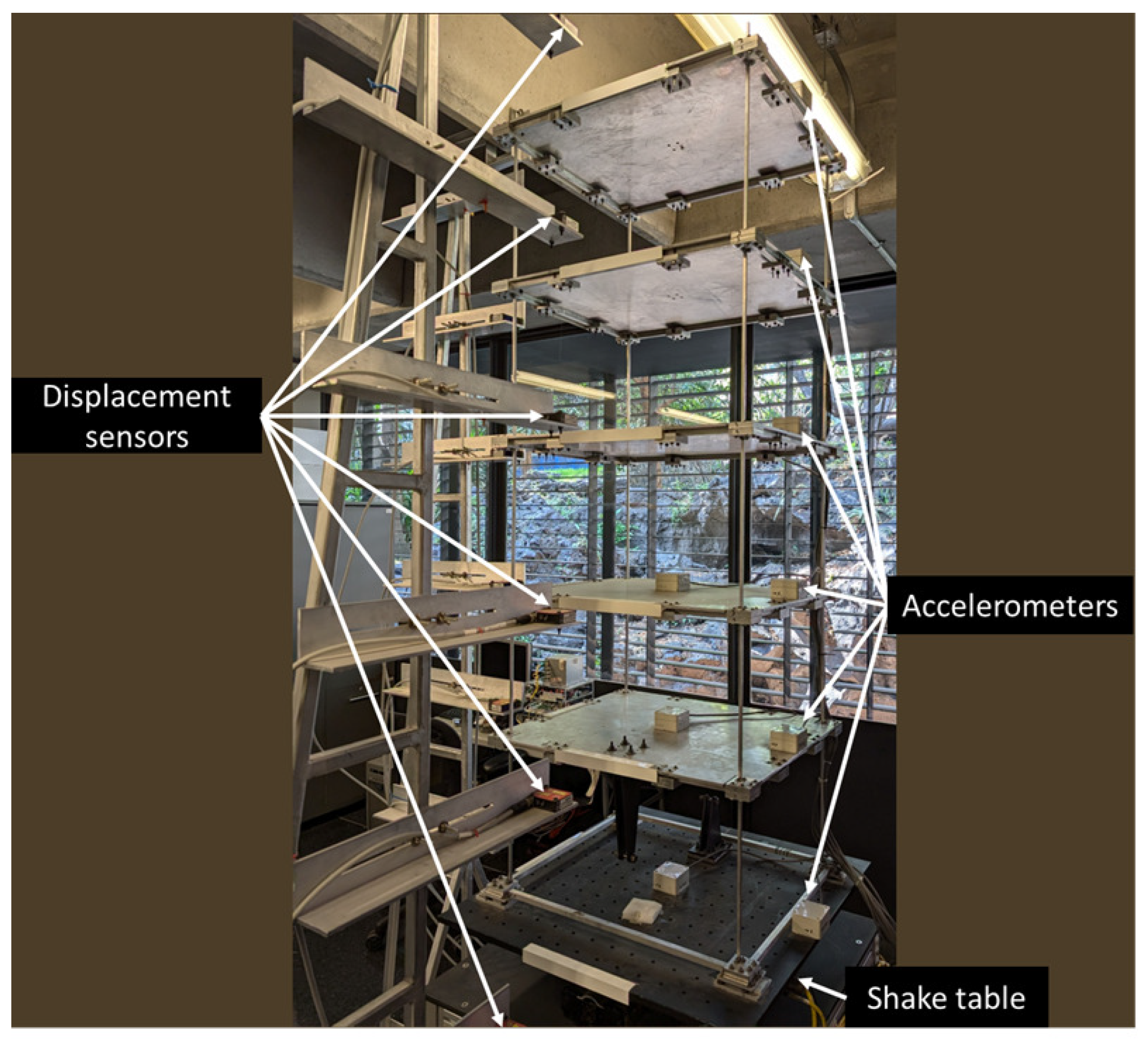
The identification was carried out with experimental data from a reduced-scale five-story building prototype made of aluminum, as shown in Figure 1. Each floor is made up of four columns, three of them made of brass with a square cross section with dimensions of 0.635 cm × 0.635 cm and a height of 36 cm, while the prototype of the building has dimensions of 60 × 50 × 180 cm. The floors consist of an aluminum sheet with adaptations on their sides for measurements, above these sheets, accelerometers are placed on the center and on one side of each floor. In addition, on the first floor. It should be noted that during its assembly, each of the masses of the components was weighed to obtain the concentrated mass of each floor; the measured masses are $M=\mathrm{diag}(\left[\begin{array}{ccccc}11.773& 9.17& 9.14& 9.12& 9.08\end{array}\right])$. Additionally, the reduced-scale structure is equipped with non-inertial accelerometers (model ADXL203E) by Analog Devices Inc., Wilmington, MA, USA. with a measurement range of $\pm 1.7$ g and a gain of 0.168 g/V per floor. It also uses laser sensors by Micro-Epsilon, Ortenburg, Germany (model OptoNCDT 1302-200) with a 20 cm range and a gain of 2.511 cm/V for floor displacement. The structure is mounted on a shake table with Parker servomotors (model 406T03LXR), offering a maximum acceleration of 5 g, a speed of 3 m/s, a position resolution of 5 μm, and a free displacement of 250 mm. All devices are connected to a computer with Simulink by MATLAB via two PCI-6221-M series boards by National Instruments, Austin, TX, USA with a 1 ms sampling time.

Although the sensors have an analog filter in their physical implementation, they require the signal to be filtered, which is carried out by the low-pass filter expressed as a transfer function.

$$F\left(s\right)={\displaystyle \frac{{\omega }_c^2}{s^2+\frac{{\omega }_c}{Q_c}s+{\omega }_c}},$$

(15)

where s represents a complex variable in the Laplace domain, $Q_c$ is a quality factor defined as 0.707, and ${\omega }_c$ is the cut-off frequency, which, considering the Fourier transform, is set to values of 6 Hz and 20 Hz for the optical and MEMS sensors, respectively. As mentioned before, the structure does not have a velocity sensor to measure each floor’s deformation speed. Therefore, the velocity on each floor is estimated from the measured positions through the following filter:

$$F\left(s\right)={\displaystyle \frac{{\omega }_c^{2}s}{s^2+\frac{{\omega }_c}{Q_c}s+{\omega }_c}}.$$

(16)

The north–south component of the seismic acceleration signal measured during the Mexico City earthquake in 1985 serves as the excitation source for the experimental structure. The parameters and state of this structure are estimated through the parametric identification approach outlined in Section 2. The amplitude of this seismic excitation is adjusted to align it with the scale of the structure. This excitation signal has sufficient complexity to facilitate the identification of the structural parameters, thereby satisfying the condition of adequate richness. Furthermore, it is important to note that the dataset utilized for the optimization was carefully selected based on five experiments conducted using the Mexico City 1985 earthquake as seismic excitation, all yielding comparable results.

4.2. Obtained Parameters

To obtain the parameters $\theta$ in the objective function specified in Equation (4), the weighting coefficients ${\eta }_1$ and ${\eta }_2$ were empirically set to 1000 and 100, respectively, following a structured sensitivity analysis. Although the selection was informed by trial and error, the process involved evaluating a grid of candidate values and observing their influence on convergence behavior across multiple runs. These weights were chosen to ensure that both displacement and velocity components contributed meaningfully to the objective function, without causing instability or premature convergence. An improper weighting balance was observed to induce algorithmic bias toward local optima, particularly for methods with limited exploratory dynamics. Therefore, careful tuning was essential to preserve the global search capabilities of all algorithms. The robustness of the selected configuration was verified through repeated trials, showing consistent parameter identification outcomes.

Table 3. Parameters on each floor.

Method	GA	PSO	QGA	QPSO	QNSGA-II	QDE	QSA
$k_1$	8555.9	8880.1	8378.9	9248.7	8204.6	8803.3	8158.4
$k_2$	8440.9	8292.8	8362	7979.9	8244.3	8434.2	8162.8
$k_3$	8040.8	7784.5	8289.7	7917.9	8228.5	7873.9	8160.8
$k_4$	8395.7	8414.9	8209.9	8264.1	8261	8745.1	8147.5
$k_5$	8379.2	8112.0	8211.6	7955.7	8249.8	7940	8135.1
$c_1$	25.56	30.30	20.46	29.97	25.25	21.99	24.61
$c_2$	15.34	18.18	18.08	16.09	24.38	21.39	24.53
$c_3$	16	10.90	18.03	16	24.87	22.26	24.52
$c_4$	22.27	15.04	17.91	16.03	24.91	24.15	24.48
$c_5$	31.01	21.02	17.38	23.54	24.61	24.81	24.42

delineates the optimal parameters identified from 30 independent trials of each optimization algorithm, with reference to the minimum value of the objective function as specified in Equation (4). These parameter values are subject to variation due to the optimization process, wherein each trial may converge to a local minimum within the solution space of the objective function. It is important to highlight that the damping coefficient poses a significant challenge in any deterministic or metaheuristic parametric identification system and may exhibit inconsistencies [28]. The experiments were performed in MATLAB 2024b and a parallel computing environment on a system equipped with an AMD EPYC 7601 processor (64 cores, 64 threads), 256 GB of RAM, and a Tesla M4 GPU with Maxwell 2.0 architecture and 1024 CUDA cores.

For the algorithms test, if not mentioned before, the maximum iterations or generations are selected as 200, the constraint tolerance is $1\times {10}^{-6}$, and the lower bounds are $lb=[5000,5000,5000,5000,5000,0,0,0,0,0],$ according to the conditions of a civil structure defined according to Equation (2). The upper bounds determined from prior assessments have been established as

$$ub=[12,000,12,000,12,000,12,000,12,000,100,100,100,100,100],$$

and an initial particle or gen as

$$\theta \left(t_0\right)=[8400,8400,8400,8400,8400,24,24,24,24,24].$$

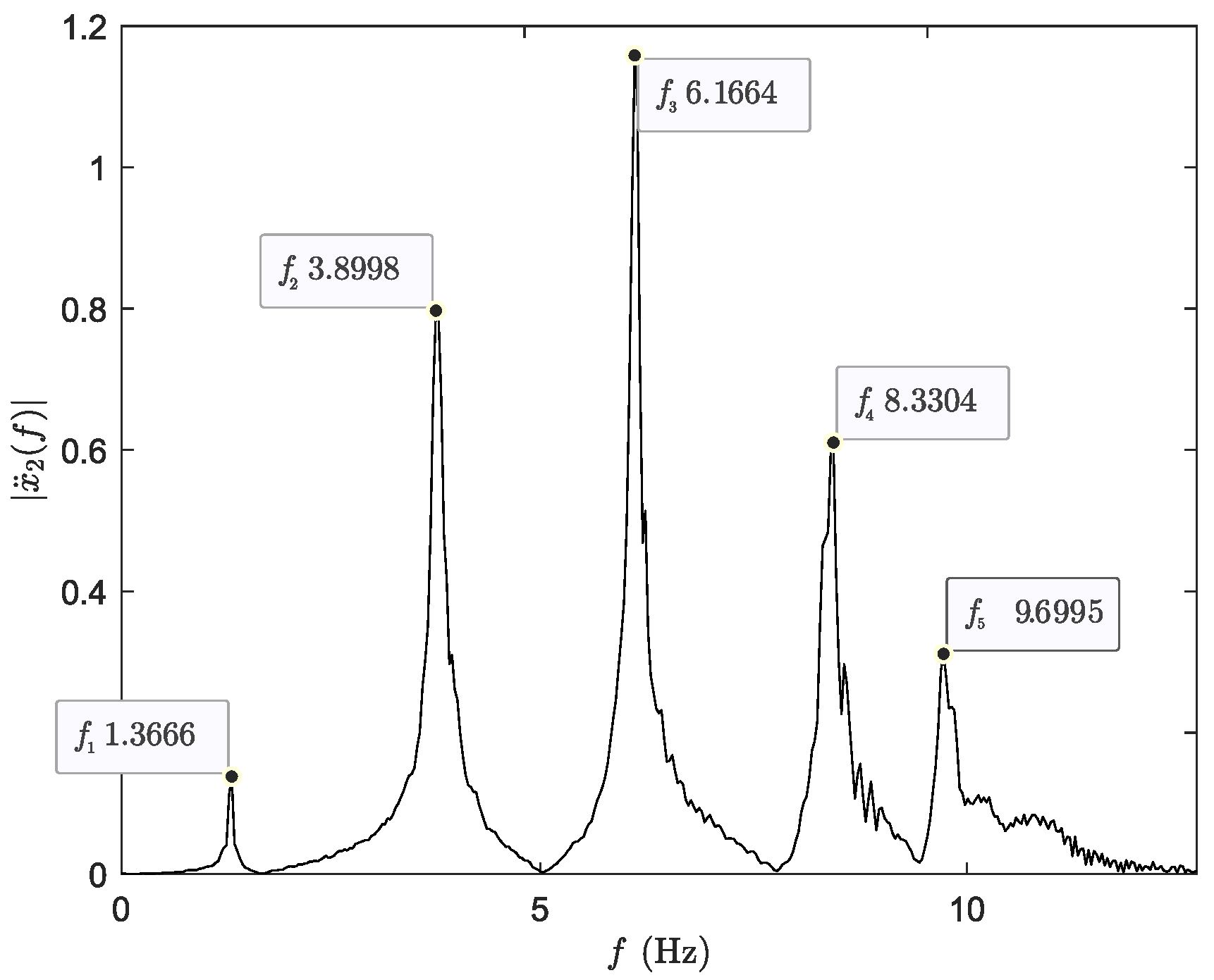
The relationship between stiffness and damping can be expressed in terms of natural frequencies via an eigenvalue problem, as noted in [28]. These frequencies can be experimentally estimated by analyzing the acceleration spectrum from a chirp signal that sweeps from 0.1 to 12 Hz over 20 s. The five natural frequencies are derived using the Fourier Transformation (FT) on acceleration records from the second story, as shown in Figure 2.

The natural frequencies estimated from the parameters in Table 3 and those from the chirp excitation test in Figure 2 are summarized in

Table 4. Natural frequency on each floor.

Method	FT 1	GA	PSO	QGA	QPSO	QNSGA-II	QDE	QSA
$f_1$	1.36	1.36	1.36	1.36	1.37	1.36	1.37	1.35
$f_2$	3.89	3.89	3.89	3.86	3.91	3.85	3.91	3.83
$f_3$	6.16	6.00	5.96	5.98	5.96	5.96	5.96	5.93
$f_4$	8.33	7.85	7.78	7.81	7.71	7.79	7.81	7.74
$f_5$	9.69	9.11	9.03	9.10	8.99	9.09	9.11	9.04
MSE	-	0.12	0.15	0.13	0.18	0.14	0.13	0.17

¹ FT is the amplitude spectrum of the Fourier transformation.

. This table includes the mean squared error (MSE) between the experimental chirp signal and the estimated frequencies, providing a metric for evaluating the reliability of the parameters with an error of less than 0.18.

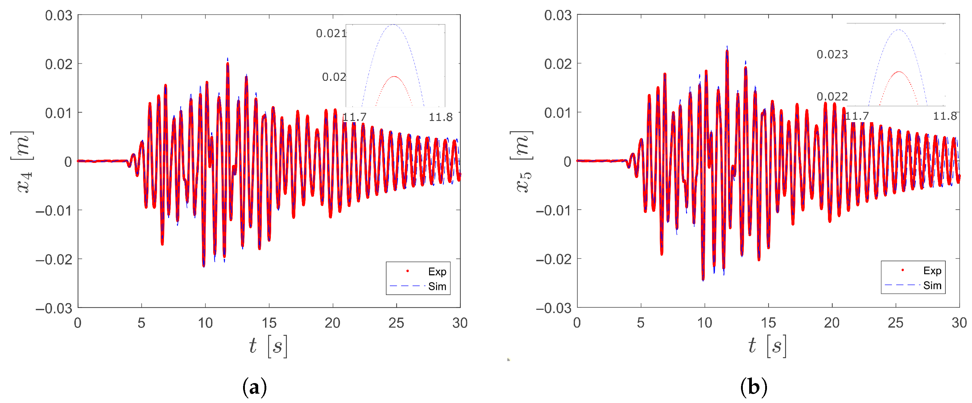
Figure 3 presents a comparison of displacement time histories, aligning experimental measurements (red dots) with model predictions (blue lines) derived from parameters optimized using PSO. In this figure, other simulated displacements are not displayed due to their similarity; they will be included in the subsequent statistical analysis, which will show the optimal parameters for the displacement history. Close alignment validates the accuracy of the identified structural parameters and demonstrates the proposed methodology’s effectiveness in capturing the structure’s dynamic behavior.

4.3. Statistical Analysis

In this segment, the parameters obtained in Section 4.2 for each optimization algorithm are statistically analyzed. Statistical validation is a fundamental pillar in the evaluation of the performance of optimization models. In this regard, refs. [33,34,35] present a comprehensive approach based on machine learning, where quantitative validation through error metrics and correlations ensures the reliability of models in complex environments.

Evaluating optimization models for structural response during seismic events needs effective error metrics to quantify discrepancies between simulated and observed data. The following performance criteria are used to assess the efficiency and accuracy of identified parameters for each floor. Firstly, the mean squared error (MSE) heavily penalizes larger deviations due to the squared term, making it effective for identifying significant errors in structural displacement predictions. This characteristic is useful when outliers are crucial for assessing the model’s performance. The MSE can be defined as

$$\mathrm{MSE}={\displaystyle \frac{1}{N}}\sum _{i=1}^N{\left(x_i-{\widehat{x}}_i\right)}^2,$$

(17)

where $x_i$ and ${\widehat{x}}_i$ refer to the experimentally measured signal and its estimation, respectively, with N as the total sample count. Secondly, the root mean squared error (RMSE) offers a precise error measure in the same units as the original data. Unlike MSE, RMSE reduces the impact of squared error growth, making it more applicable for comparing deviations with observed structural displacements and velocities. The RMSE can be expressed as

$$\mathrm{RMSE}={\displaystyle \frac{1}{N}}\sum _{i=1}^N\sqrt{{\left(x_i-{\widehat{x}}_i\right)}^2}.$$

(18)

Thirdly, the coefficient of determination ($R^2$) indicates the proportion of variance in observed data explained by the model. A high $R^2$ suggests that the optimization effectively captures structural behavior under seismic loads and is useful for comparing models and their predictive capabilities. $R^2$ can be represented as

$${\mathrm{R}}^2=1-{\displaystyle \frac{{\sum }_{i=1}^N{\left(x_i-{\widehat{x}}_i\right)}^2}{{\sum }_{i=1}^N{\left(x_i-{\overline{x}}_i\right)}^2}},$$

(19)

where ${\overline{x}}_i$ indicates the mean value of the signal $x_i$. Finally, the mean absolute error (MAE) is a more intuitive and robust measure than the MSE or RMSE, as it is less sensitive to large outliers. Defined based on absolute differences, the MAE is particularly useful in scenarios where overall model consistency is prioritized over large deviations. The MAE can be defined as

$$\mathrm{MAE}={\displaystyle \frac{1}{N}}\sum _{i=1}^N|x_i-{\widehat{x}}_i|.$$

(20)

4.3.1. Statistical Analysis of Stiffness and Damping Coefficients

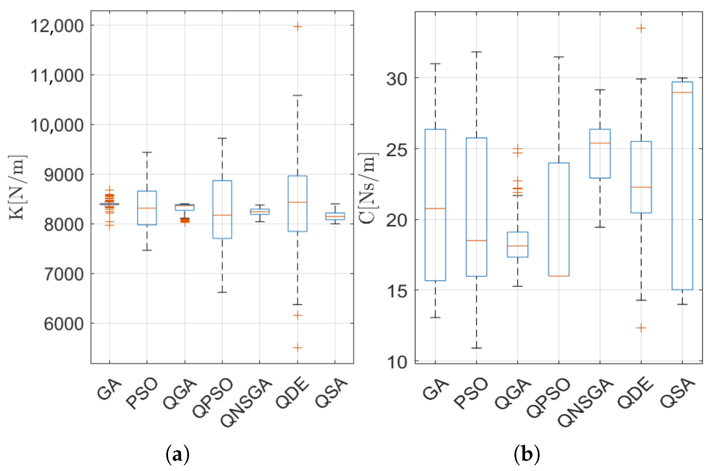
Before conducting error analysis, it is essential to evaluate the dispersion of obtained parameters to ensure the integrity of our findings. Boxplot visualizations offer insights into the accuracy and variability of each model, facilitating a comparative assessment of their predictive capabilities. This analysis will identify the most effective models and highlight potential limitations in others.

The analysis of normality revealed that, unlike MSE, RMSE, and MAE, the $R^2$ metric did not consistently follow a normal distribution across all floors and algorithms. This deviation has important implications for the choice of statistical tests. While ANOVA and post hoc comparisons assume normality and homogeneity of variance, the use of multiple metrics in parallel, each satisfying these assumptions, provides partial mitigation. Additionally, the robustness of the overall validation framework was enhanced by the use of Bootstrap resampling and Borda count analysis, which are non-parametric by nature. Although non-parametric alternatives such as the Kruskal–Wallis test were not implemented in this study, they are considered valuable for future extensions, especially when working with field data where residual distributions may be more irregular.

The analysis reveals that floor 4 has a distinct correlation pattern compared to the other floors, indicating unique structural characteristics. The correlation matrix shows that $k_4$ and $c_4$ exhibit lower interactions with other parameters, likely due to optimization variations rather than structural disconnection. The optimization results demonstrate that $c_4$ varies significantly across methods (15.04 for PSO to 24.91 for QNSGA-II), emphasizing the influence of algorithm choice on damping distribution. While $k_4$ remains stable, its interaction with damping coefficients varies, suggesting areas for optimization refinement. These findings will be further investigated to improve parameter distribution and structural response.

In this regard, Figure 4 presents the variability and distribution of stiffness (K) and damping (C) coefficients across different optimization models. The left boxplot illustrates the variability of K values, indicating notable differences among the evaluated models. Certain algorithms display larger interquartile ranges, suggesting a greater degree of variability in their stiffness estimations, while others exhibit more consistent values. The identification of outliers suggests that specific iterations resulted in extreme stiffness outcomes. The boxplot for GA (Genetic Algorithm) applied to the coefficients of K exhibits a narrow interquartile range (IQR), indicating that most values are tightly clustered. However, it also presents numerous outliers above and below the central distribution. This suggests that while the majority of the data points remain stable, fluctuations or anomalies cause certain extreme values. These variations may be attributed to numerical instability, unmodeled effects, or irregularities in the GA optimization process, where convergence might not always lead to a completely stable solution.

The boxplot for QGA (Quantum Genetic Algorithm) applied to the coefficients of K also shows a small IQR, meaning the dataset is concentrated around a specific range. However, it is asymmetrically skewed downward, with several lower outliers. This suggests that some optimization iterations resulted in unexpectedly low parameter values, possibly due to quantum-inspired variations in the search space. These fluctuations could stem from irregularities in quantum-inspired crossover and mutation mechanisms, leading to some solutions being significantly lower than expected. Conversely, the right boxplot presents the distribution of the damping coefficient, C, highlighting significant disparities in estimation accuracy. Some models reveal a higher degree of dispersion, indicating potential inconsistencies in parameter tuning, whereas others demonstrate relative stability. The comparative analysis of the two distributions indicates that while certain models may show consistent performance for one parameter, they may exhibit increased variability for the other.

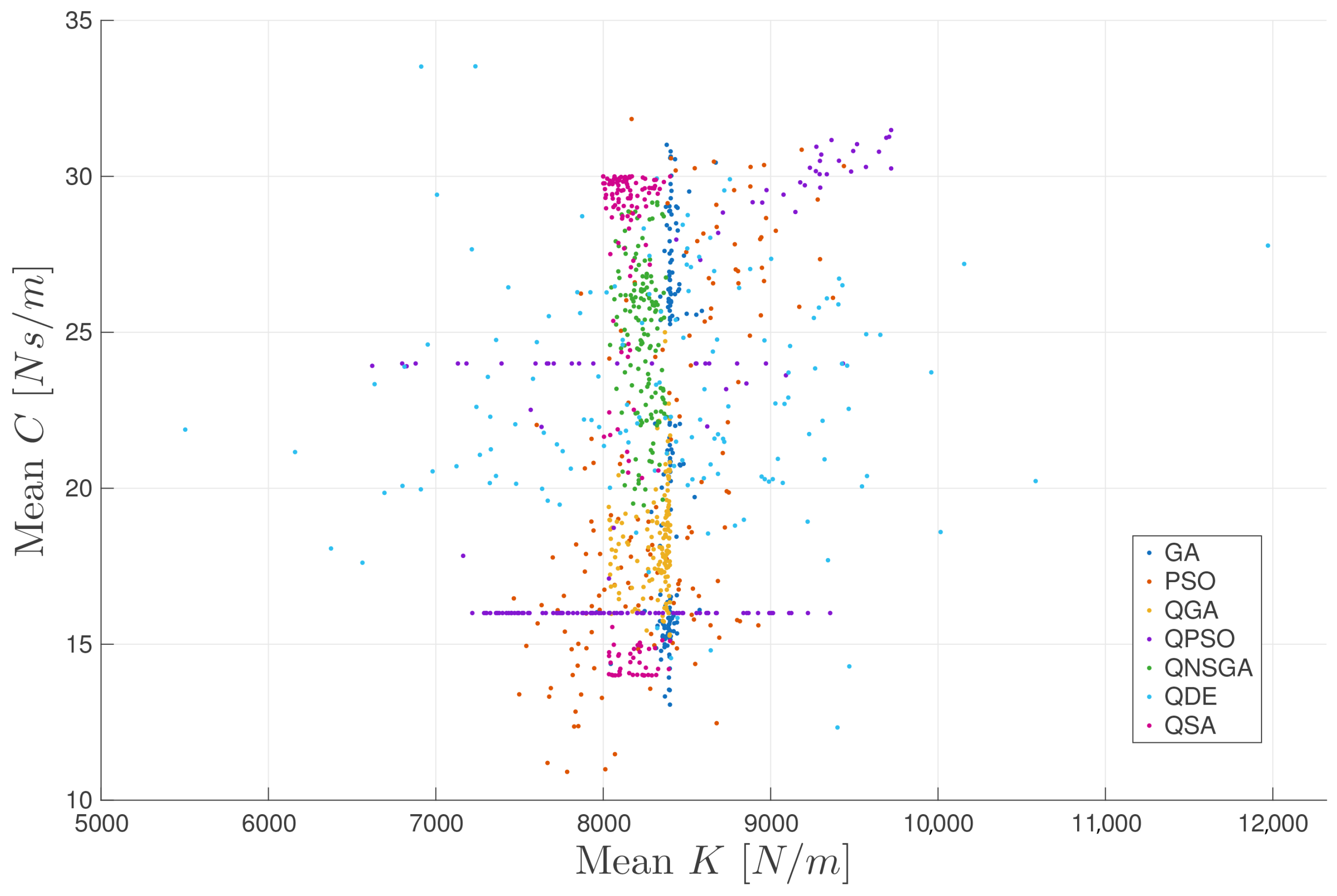
Moreover, the relationship between stiffness (K) and damping (C) coefficients across various optimization models is shown in Figure 5. The distribution of points indicates a significant spread in both parameters, suggesting considerable variability in the estimation process. While some models cluster around specific ranges, others exhibit a broader dispersion, reflecting inconsistent parameter tuning. The presence of distinct color-coded groups highlights differences among optimization techniques, with certain models tending toward higher damping values while others concentrate on lower values. Additionally, the vertical dispersion of points suggests that, for similar K values, damping coefficients can vary significantly, implying that stiffness alone may not be a strong predictor of damping behavior. The results emphasize the need for a balanced optimization strategy that accounts for both parameters to ensure integrity in structural applications. The dispersion of k values in the error metrics of QGA suggests that this method explores a broader solution space, leading to greater variability in the optimized stiffness parameters.

In addition, Figure 6 presents a correlation matrix that provides a quantitative assessment of the relationships between stiffness (K) and damping (C) coefficients across different optimization models. The color-coded heatmap visually represents the correlation coefficients, where values closer to 1 or −1 indicate strong positive or negative correlations, respectively, while values near 0 suggest weak or no correlation. In fact, diagonal elements confirm the expected perfect self-correlation (r = 1). Certain stiffness parameters (K) exhibit moderate correlations with damping coefficients (C), which may indicate structural dependencies influenced by the optimization algorithm. However, the variability in correlation values across different parameters suggests that stiffness and damping are not universally dependent, reinforcing the need for model-specific tuning.

Finally, the probability distributions of stiffness (K) and damping (C) coefficients across different optimization models are illustrated in Figure 7. The left panel shows that K follows an unimodal distribution, with most values concentrated around a central peak, indicating that stiffness values tend to cluster within a specific range. The narrow spread suggests relatively low variability in K compared to C. The right panel presents the distribution of damping coefficients (C), which exhibits an irregular shape with multiple peaks. This suggests that different optimization models lead to varying damping values, potentially influenced by the algorithm’s characteristics and parameter-tuning strategies. The comparison of both distributions highlights the different nature of these parameters, where stiffness remains more stable while damping values exhibit greater dispersion and variability across the models.

4.3.2. Normality Analysis Using the Shapiro–Wilk Test

The normality of residuals for four key error metrics—mean squared error (MSE), root mean squared error (RMSE), mean absolute error (MAE), and the coefficient of determination ($R^2$)—was evaluated across different optimization models and structure floors. The Shapiro–Wilk normality test was conducted separately for each metric in each model and at every structure floor to determine whether the residuals followed a normal distribution [36].

Table 5. Full normality Analysis (Shapiro–Wilk test).

Metric	Statistic	GA	PSO	QGA	QPSO	QNSGA-II	QDE	QSA
$MSE$	Normal/Not Normal	5/0	5/0	5/0	5/0	5/0	5/0	5/0
	p-Max	0.8168	0.7969	0.8260	0.8013	0.8326	0.8073	0.8448
	p-Min	0.7982	0.7710	0.8196	0.7698	0.8209	0.7533	0.8277
$RMSE$	Normal/Not Normal	5/0	5/0	5/0	5/0	5/0	5/0	5/0
	p-Max	0.7906	0.7958	0.8102	0.8114	0.8066	0.8017	0.7981
	p-Min	0.7746	0.7674	0.7999	0.7810	0.7957	0.7438	0.7455
$MAE$	Normal/Not Normal	5/0	5/0	5/0	5/0	5/0	5/0	5/0
	p-Max	0.8082	0.8106	0.8269	0.8245	0.8151	0.8066	0.7999
	p-Min	0.7970	0.7907	0.8179	0.7988	0.7953	0.7515	0.7436
$R^2$	Normal/Not Normal	1/4	5/0	4/1	4/1	5/0	4/1	5/0
	Not Normal Floors	1, 3, 4, 5	-	3	2	-	4	-
	p-Max	0.0919	0.6781	0.6914	0.8671	0.9241	0.5959	0.9261
	p-Min	0.0203	0.2767	0.0427	0.0456	0.0551	0.0050	0.0679

summarizes the Shapiro–Wilk normality test applied to four error metrics—MSE, RMSE, MAE, and $R^2$—across various optimization methods (GA, PSO, QGA, QPSO, QNSGA-II, QDE, QSA). The row “Normal/Not Normal” indicates the count of trials where the metric’s residuals were found to follow (or deviate from) a normal distribution. The results of MSE, RMSE, and MAE show complete normality (5/0), suggesting that all tested instances for these metrics align with a normal distribution. In contrast, the $R^2$ metric displays mixed outcomes, with entries such as “1/4” or “4/1,” indicating a subset of tests where the normality assumption was unmet. The corresponding p-values (p-Max and p-Min) corroborate these findings. For MSE, RMSE, and MAE, the p-values consistently exceed the conventional 0.05 threshold, thus failing to reject the null hypothesis of normality. However, for $R^2$, some p-values fall below 0.05, implying that those $R^2$ residuals deviate significantly from a normal distribution.

The results indicate that while MSE, RMSE, and MAE are consistently normal across all optimization methods, $R^2$ shows sensitivity to the method used, sometimes behaving non-normally. This is important when selecting statistical analyses or modeling techniques that assume normal residuals. Additionally, the assumption of homogeneity of variance in error metrics is critical; significant variance across structure floors can lead to inconsistencies in predictive performance. This variability may affect the stability and reliability of the optimization process in structural response modeling under seismic excitation.

4.3.3. Variance Homogeneity Using Levene and Bartlett Tests

To assess the homogeneity of variance, Levene’s and Bartlett’s tests were conducted on four key error metrics. The Levene test is particularly useful in this context, as it does not require a normal distribution and is robust to deviations from normality. In contrast, the Bartlett test assumes normally distributed data and provides a stricter evaluation criterion when this assumption holds [37,38]

Table 6. Evaluation of variance homogeneity for error metrics across optimization models and floors.

Metric	Test	Floor 1	Floor 2	Floor 3	Floor 4	Floor 5
$MSE$	Levene	0.7856	0.7504	0.6849	0.0110	0.7610
	Bartlett	0.9313	0.9256	0.8933	0.0630	0.9319
$RMSE$	Levene	0.9888	0.9860	0.9812	0.4728	0.9881
	Bartlett	0.9985	0.9983	0.9975	0.8400	0.9986
$MAE$	Levene	0.9533	0.9537	0.9425	0.3057	0.9603
	Bartlett	0.9922	0.9935	0.9909	0.7195	0.9946
$R^2$	Levene	0.5316	0.2042	0.0997	0.0013	0.6231
	Bartlett	0.2328	0.0321	0.0080	0.0005	0.2080

summarizes the p-values obtained for both tests across all floors. A p-value above 0.05 indicates that variance homogeneity is maintained, whereas a p-value below 0.05 suggests significant differences in variance, implying potential inconsistencies in model performance across floors.

The primary goal of these tests is to assess the consistency of error dispersion across optimization models and structural levels. The MSE and MAE metrics generally show homogeneous variance across all floors, as indicated by p-values above 0.05 in both the Levene and Bartlett tests. However, floor 4 shows a notable exception for MSE, with a p-value of 0.0110, indicating significant deviation from homogeneity. This suggests certain optimization models produce highly variable errors at this level due to nonuniform performance in response to seismic activity. In contrast, the RMSE metric maintains stable variance across all floors, reinforcing its reliability. The $R^2$ metric, however, shows heterogeneity in floors 2, 3, and 4, with p-values below 0.05, indicating differing levels of predictive consistency. These inconsistencies highlight the need for further investigation into the variance sources, particularly for MSE in floor 4 and for $R^2$ on multiple floors, suggesting that some optimization models may require adjustments for improved stability.

4.3.4. Error Metrics Analysis Using ANOVA and Post Hoc (Tukey–Bonferroni) Test

The examination of error metrics within the context of ANOVA, along with the application of post hoc tests such as Tukey’s and Bonferroni’s methods, is crucial for identifying significant differences among groups while mitigating the risk of statistical errors [39].

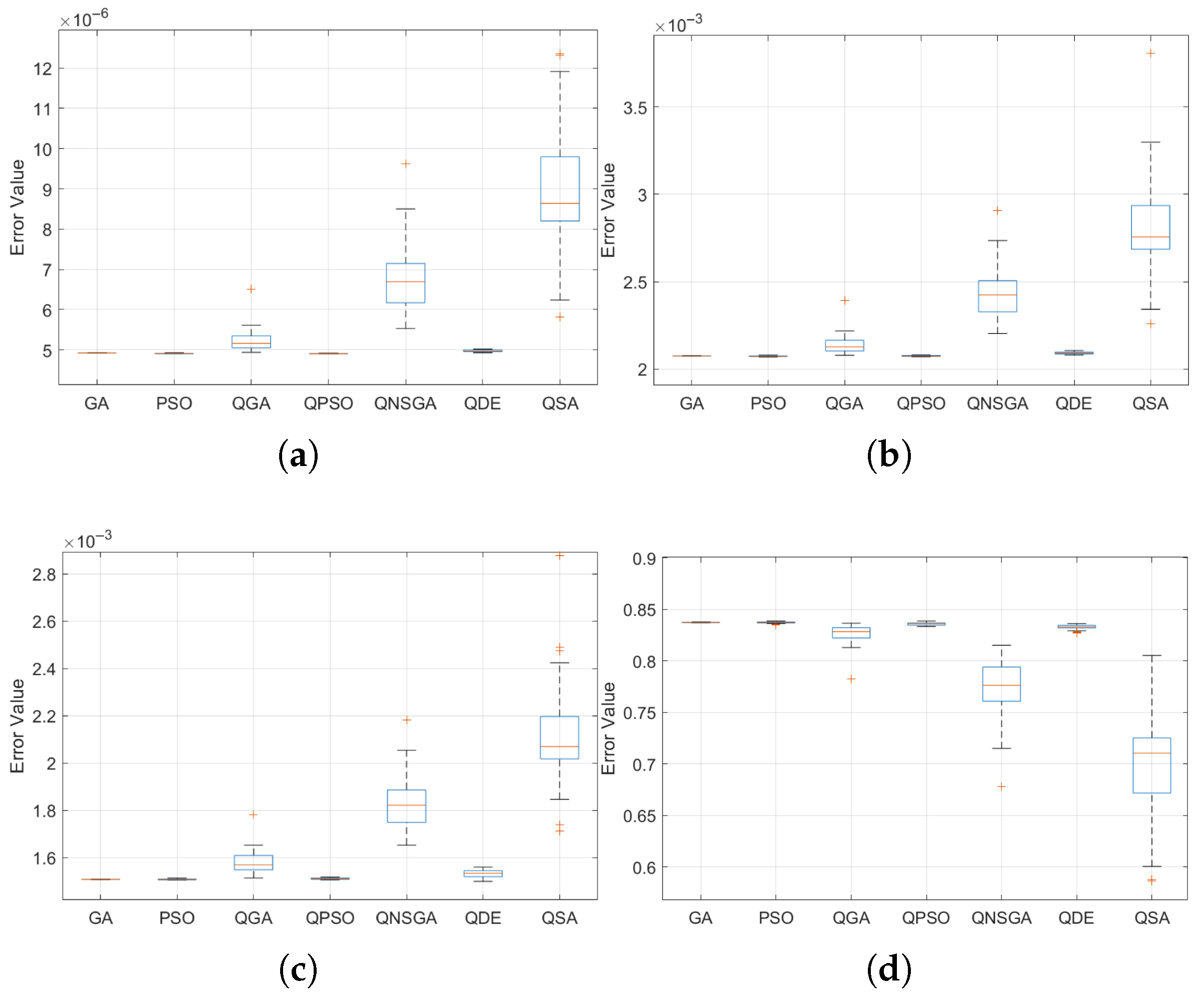
In this context, the first three subplots in Figure 8 illustrate the distribution of MSE, RMSE, and MAE, critical prediction accuracy indicators. Lower values in these metrics signify superior performance, as they represent a closer alignment between the estimated and actual values. Notably, the GA, PSO, and QGA models demonstrated the lowest MSE, RMSE, and MAE values, indicating enhanced precision and consistency in their predictions. Furthermore, these models exhibited narrower interquartile ranges (IQRs), indicative of greater stability and reduced variability. In contrast, QNSGA-II and QSA produced significantly higher error values, accompanied by wider interquartile ranges and a greater number of outliers. These findings suggest heightened variability, which may stem from inefficient parameter tuning or suboptimal convergence properties. The QDE model displayed intermediate performance, yielding moderate error values and variability. This suggests that, while it may not be the most precise option, the QDE model can provide a balance between predictive accuracy and robustness.

The $R^2$ metric provides information on the proportion of variance in the data explained by each model. GA, PSO, and QGA demonstrated consistently high $R^2$ values close to 1, confirming their superior ability to model the underlying patterns in the dataset. In contrast, QNSGA and QSA showed considerably lower $R^2$ values, further corroborating their higher error metrics and suggesting a weaker predictive capacity.

4.3.5. Student’s t-Test with a Bonferroni Correction

A rigorous evaluation of optimization algorithms is essential to determine their effectiveness in parametric identification tasks, particularly in complex engineering applications. Given the inherent variability and computational demands of heuristic and metaheuristic approaches, a robust statistical validation framework is necessary to assess their accuracy, stability, and predictive reliability. To this end, a pairwise Student’s t-test with Bonferroni correction was conducted to quantify the statistical significance of performance differences between competing algorithms [40]. The analysis focuses on four key error metrics: mean squared error (MSE), root mean squared error (RMSE), mean absolute error (MAE), and the coefficient of determination ($R^2$). A model is considered statistically superior if at least three out of the four metrics favor its performance, while cases where two metrics indicate superiority and two show no significant differences are classified as equivalent.

In

Table 7. Pairwise Student’s t-test with Bonferroni correction for MSE, RMSE, MAE, and $R^2$.

Model Ref	Compared Model	p-Value (MSE)	p-Value (RMSE)	p-Value (MAE)	p-Value (${\mathit{R}}^2$)	Conclusions
GA	PSO	1.249 $\times {10}^{-12}$	1.417 $\times {10}^{-4}$	1.928 $\times {10}^{-23}$	4.322 $\times {10}^{-1}$	GA is better
GA	QGA	5.781 $\times {10}^{-7}$	1.838 $\times {10}^{-7}$	1.040 $\times {10}^{-3}$	1.696 $\times {10}^{-7}$	GA is better
GA	QPSO	1.928 $\times {10}^{-23}$	6.040 $\times {10}^{-1}$	1.095 $\times {10}^{-16}$	1.723 $\times {10}^{-6}$	GA is better
GA	QNSGA	1.379 $\times {10}^{-16}$	1.876 $\times {10}^{-18}$	1.876 $\times {10}^{-18}$	3.541 $\times {10}^{-15}$	GA is better
GA	QDE	3.585 $\times {10}^{-16}$	7.769 $\times {10}^{-19}$	1.484 $\times {10}^{-15}$	9.686 $\times {10}^{-16}$	GA is better
GA	QSA	1.637 $\times {10}^{-15}$	1.230 $\times {10}^{-18}$	1.095 $\times {10}^{-18}$	2.421 $\times {10}^{-7}$	GA is better
PSO	GA	4.322 $\times {10}^{-1}$	1.417 $\times {10}^{-4}$	1.928 $\times {10}^{-23}$	4.322 $\times {10}^{-1}$	Equivalent
PSO	QGA	4.322 $\times {10}^{-1}$	9.148 $\times {10}^{-8}$	6.180 $\times {10}^{-14}$	1.722 $\times {10}^{-6}$	QGA is better
PSO	QPSO	4.322 $\times {10}^{-1}$	3.036 $\times {10}^{-2}$	1.977 $\times {10}^{-7}$	1.723 $\times {10}^{-6}$	Equivalent
PSO	QNSGA	4.322 $\times {10}^{-1}$	1.280 $\times {10}^{-18}$	7.599 $\times {10}^{-13}$	3.541 $\times {10}^{-15}$	QNSGA is better
PSO	QDE	4.322 $\times {10}^{-1}$	2.280 $\times {10}^{-18}$	5.507 $\times {10}^{-15}$	9.686 $\times {10}^{-16}$	QDE is better
PSO	QSA	4.322 $\times {10}^{-1}$	1.095 $\times {10}^{-18}$	1.327 $\times {10}^{-10}$	2.421 $\times {10}^{-7}$	QSA is better
QGA	GA	1.696 $\times {10}^{-7}$	1.417 $\times {10}^{-4}$	1.928 $\times {10}^{-23}$	4.322 $\times {10}^{-1}$	GA is better
QGA	PSO	1.696 $\times {10}^{-7}$	9.148 $\times {10}^{-8}$	6.180 $\times {10}^{-14}$	1.722 $\times {10}^{-6}$	QGA is better
QGA	QPSO	1.696 $\times {10}^{-7}$	3.036 $\times {10}^{-2}$	1.977 $\times {10}^{-7}$	1.723 $\times {10}^{-6}$	Equivalent
QGA	QNSGA	1.696 $\times {10}^{-7}$	1.280 $\times {10}^{-18}$	7.599 $\times {10}^{-13}$	3.541 $\times {10}^{-15}$	QNSGA is better
QGA	QDE	1.696 $\times {10}^{-7}$	2.280 $\times {10}^{-18}$	5.507 $\times {10}^{-15}$	9.686 $\times {10}^{-16}$	QDE is better
QGA	QSA	1.696 $\times {10}^{-7}$	1.095 $\times {10}^{-18}$	1.327 $\times {10}^{-10}$	2.421 $\times {10}^{-7}$	QSA is better

, the statistical findings indicate that the Genetic Algorithm (GA) demonstrates superior performance compared to Particle Swarm Optimization (PSO) and Quantum Particle Swarm Optimization (QPSO), consistently achieving lower error values (MSE, RMSE, and MAE) and higher predictive accuracy ($R^2$). However, when benchmarked against quantum-inspired algorithms such as the Quantum Non-Dominated Sorting Genetic Algorithm (QNSGA) and Quantum Differential Evolution (QDE), GA exhibits reduced efficiency, suggesting that quantum-based approaches enhance stability and precision in parametric identification. In contrast, PSO shows moderate competitiveness, achieving equivalence in several comparisons but failing to outperform quantum-hybrid models. These results suggest that while swarm-based optimization techniques can be effective under specific conditions, their precision remains suboptimal when compared to quantum-enhanced strategies. The QNSGA and QDE emerge as the most robust methodologies, consistently yielding superior results across all metrics. Their statistical advantage over traditional heuristic approaches highlights the potential of quantum-inspired optimization techniques for improving parametric identification in structural engineering applications.

4.3.6. Coefficient of Variation in Bootstrap Rankings

To further evaluate the stability of the optimization models, a Bootstrap ranking analysis was conducted. Bootstrap is a statistical resampling technique that allows for assessing the variability and consistency of model rankings across multiple trials. This method provides insights into how reliably each optimization algorithm performs under different sampling conditions [41].

The analysis focuses on three key metrics for evaluating model performance. The mean ranking indicates the average position of each model across multiple bootstrap iterations, with lower values signifying better performance. The standard deviation measures the variability of rankings across resampled datasets, where smaller values indicate more stable rankings. The coefficient of variation (CV), the ratio of standard deviation to mean ranking, normalizes dispersion. A lower CV suggests consistent ranking despite data fluctuations, while a higher CV indicates greater variability in performance. CV can be defined as

$$CV={\displaystyle \frac{\mathrm{Standard}\mathrm{Deviation}}{\mathrm{Mean}\mathrm{Ranking}}}$$

(21)

Table 8. Coefficient of variation (CV) in Bootstrap rankings.

Model	Mean Ranking	Std. Dev.	CV
GA	3.235	1.9661	0.60777
PSO	3.974	1.9553	0.49202
QGA	4.140	1.9709	0.47605
QPSO	3.969	2.0080	0.50592
QNSGA-II	4.068	1.9481	0.47889
QDE	3.905	1.9457	0.49826
QSA	4.709	1.9282	0.40948

summarizes the Bootstrap ranking analysis results, highlighting the stability of various optimization models. The GA has a mean ranking of 3.235 with a CV of 0.60777, indicating reasonable performance but relative instability. In contrast, the QSA model has the highest mean ranking of 4.709 and the lowest CV of 0.40948, suggesting consistency despite not having the best ranking. Among quantum-based models, QPSO shows the highest CV of 0.50592, indicating sensitivity to dataset variations. Other quantum models, including QGA and QDE, exhibit lower CV values (below 0.5), demonstrating more stability compared to classical methods like GA and PSO, which show moderate stability with CVs around 0.49. Overall, quantum-based models, particularly QSA and QGA, display lower ranking variability, making them more reliable for robust optimization tasks, while models with higher CV values, like GA and QPSO, are more sensitive to sampling fluctuations.

4.3.7. Borda Count Analysis

The evaluation of optimization model rankings requires a robust methodology that accounts for variability across multiple instances. To achieve this, the Borda count method was employed alongside 1000 Bootstrap iterations. This approach integrates a voting-based ranking system with resampling techniques to mitigate variability caused by data fluctuations [42]. The Borda count assigns scores based on model ranking positions across multiple instances, providing a comprehensive measure of overall performance [43]. Bootstrap enhances this evaluation by generating multiple subsamples, ensuring robustness against outliers and specific dataset conditions. By combining these two techniques, it is possible to derive a more stable and interpretable ranking structure, making it a valuable tool for comparing optimization methods in dynamic environments.

The Borda count ranking results using 1000 Bootstrap iterations reveal notable trends in model stability and ranking performance (see

Table 9. Distribution of rankings per Bootstrap iteration (Borda count).

Model	Pos1	Pos2	Pos3	Pos4	Pos5	Pos6	Pos7
GA	26.4	18.7	13.9	12.0	11.2	10.6	7.2
PSO	12.8	15.9	15.6	13.3	13.3	15.6	13.5
QGA	11.6	13.8	14.9	13.0	13.3	15.3	15.4
QPSO	14.9	14.7	12.9	15.3	13.9	13.8	14.5
QNSGA-II	11.5	15.6	15.9	15.6	13.4	15.1	12.9
QDE	14.4	14.5	14.6	14.5	13.5	16.8	11.7
QSA	8.4	10.2	13.9	16.7	18.3	13.8	23.2

). The GA model achieves the highest probability (26.4) of securing the top position, indicating strong performance across different iterations. On the other hand, QSA exhibits the lowest probability (23.2), suggesting its relative inefficiency in this evaluation. The remaining models, including PSO, QGA, QPSO, QNSGA-II, and QDE, present a more evenly distributed ranking behavior, implying moderate variability and competitive performance among them.

Integrating Borda count with Bootstrap enhances ranking robustness by minimizing data fluctuations and biases. This combination offers a stable framework for assessing model reliability, making it valuable for optimization methods in dynamic environments. The findings emphasize the need to evaluate ranking stability alongside performance metrics for better decision-making in optimization tasks.

5. Discussion

5.1. Algorithm Performance and Parameter Identification Insights

Identifying structural parameters in civil structures, such as natural frequencies and damping ratios, is essential for the design, maintenance, and safety assessment of buildings and bridges. Accurate estimation of these parameters enables early detection of structural degradation, reduces the risk of failure under dynamic loads, and supports optimized designs in terms of strength, efficiency, and cost-effectiveness. As shown in Table 3, the correct identification of stiffness and damping values contributes directly to structural health monitoring and model calibration.

In this work, a five-story linear mass–spring–damper model was used as a controlled benchmark to evaluate the performance of various optimization algorithms. Although simplified, this model captures the dominant modal dynamics and facilitates repeatable testing. Nevertheless, it omits key features of real structures, including geometric and material nonlinearities, stiffness degradation, soil–structure interaction, and non-viscous damping mechanisms. These simplifications limit direct applicability to full-scale buildings. To enhance generalizability, future work should incorporate high-fidelity finite element models and field data from instrumented structures. Additionally, adapting the objective function to account for model uncertainties and nonlinear behavior would increase the relevance of this approach for practical applications.

The performance results revealed interesting differences among algorithms. GA exhibited the highest average ranking (26.4%) according to the Borda count in Table 9, while QSA, despite achieving the lowest MSE and RMSE values, had the lowest ranking probability (23.2%). This divergence points to the distinction between accuracy and robustness. While QSA can converge to highly accurate solutions, its variability across runs reduces its overall reliability. In contrast, models such as QNSGA-II and QDE delivered more consistent results across executions, even if their mean errors were slightly higher. This reinforces the importance of evaluating both dimensions when assessing optimization performance: accuracy in individual runs and robustness across repeated trials.

A detailed analysis of the identified stiffness (K) and damping (C) coefficients revealed distinct algorithmic sensitivities toward each parameter according to Figure 7. Stiffness, which governs the natural frequencies of the structure, tends to dominate the system’s dynamic response and provides clearer optimization gradients, as shown in Figure 5. In contrast, damping primarily influences amplitude attenuation and is more challenging to estimate, particularly when velocity is derived from filtered displacement signals. Algorithms with broader exploration capabilities, such as QDE and QSA, are better suited to capture subtle damping effects, whereas others may prioritize convergence speed at the expense of sensitivity. These findings highlight the importance of designing multi-objective cost functions and validation strategies that evaluate stiffness and damping in a balanced manner.

Although the optimization strategies employed were not explicitly adapted or redesigned for the inverse problem, the analysis incorporated key characteristics specific to structural parameter identification. For instance, the differing sensitivities in the estimation of stiffness and damping coefficients revealed underlying issues such as parameter coupling and differential observability (see Figure 6). Damping estimation, in particular, was influenced by noise and the need to reconstruct velocity from filtered displacement, making it more vulnerable to variability across optimization runs. Rather than modifying the internal logic of each algorithm, the proposed evaluation framework captures these behaviors through multi-criteria assessment and statistically robust comparisons. This design enables the extraction of problem-specific insights from general-purpose algorithms and contributes to bridging method-driven exploration with problem-driven interpretation.

While a formal Pareto front was not constructed due to the scalar nature of the objective function, the trade-off between displacement and velocity errors was embedded directly into the cost design using fixed weights (1000 and 100, respectively). This approach reflects engineering priorities and enables the optimization process to balance precision in displacement tracking with the sensitivity required for accurate velocity estimation. Particularly in the case of QNSGA-II, which explores diverse solutions across objective dimensions, the algorithm implicitly samples the trade-off space even when only the weighted sum is evaluated. Although the individual error components were not retained to visualize a Pareto front, the selection of solutions and comparative performance analysis provide meaningful insight into this multi-objective behavior.

5.2. Methodological Contributions and Validation Framework

While the optimization algorithms applied in this study are not novel, the methodological contribution lies in the systematic integration of quantum-inspired metaheuristics within a unified framework for structural parameter identification. Unlike prior studies limited to isolated comparisons, the proposed approach evaluates algorithm performance across several dimensions—accuracy, robustness, and sensitivity to structural parameters—under a consistent benchmark. Furthermore, the inclusion of both parametric and non-parametric statistical analyses, including Shapiro–Wilk tests, ANOVA with post hoc corrections, Bootstrap resampling, and Borda count aggregation, enhances the rigor and reproducibility of the evaluation. This framework not only supports quantitative performance comparison but also serves as a transferable protocol for assessing optimization strategies in engineering problems characterized by uncertainty and multi-criteria behavior.

To ensure the statistical validity of the results, this study incorporated a rigorous validation framework. Normality of residuals was verified using the Shapiro–Wilk test (see Table 5), which confirmed that MSE, RMSE, and MAE were normally distributed, while $R^2$ occasionally deviated from normality. Homogeneity of variance across floors was assessed with Levene and Bartlett tests, satisfying assumptions for ANOVA. Based on these conditions, one-way ANOVA with Tukey–Bonferroni post hoc tests was used to identify significant differences among algorithms. To complement this, Bootstrap resampling (1000 iterations) was performed to compute mean rankings, standard deviation, and coefficient of variation. The Borda count method was applied as a non-parametric aggregation strategy, providing a robust comparative framework. Although non-parametric alternatives such as Kruskal–Wallis were not applied here, they are worth exploring in future studies involving more irregular or field-acquired data.

5.3. Limitations and Future Research

In terms of computational performance, quantum-inspired algorithms—especially QSA, QDE, and QNSGA-II—required substantially more runtime than classical methods. While GA and PSO completed within 15 min, quantum models often exceeded one hour due to their population-based nature and complex search dynamics. These differences, observed using high-performance computing (64-core AMD EPYC CPU and Tesla M4 GPU), currently limit the use of quantum-inspired methods in real-time monitoring. However, they remain well-suited for offline assessment and post-seismic evaluation.

From a practical standpoint, quantum-inspired algorithms—despite requiring longer execution times—offer highly accurate and stable solutions that are particularly suitable for non-real-time applications, such as post-seismic structural assessments, calibration of digital twins, and structural health diagnostics in critical infrastructure. In contrast, classical methods like GA and PSO may be preferred for real-time scenarios due to their faster convergence. This differentiation highlights the importance of aligning algorithm selection with the temporal and computational constraints of the target engineering application.

While quantum-inspired algorithms did not consistently outperform classical methods across all error metrics—particularly in RMSE and MAE—their performance was more stable across repeated trials. This was evidenced by lower coefficients of variation and tighter bootstrap ranking distributions. In scenarios involving noisy or incomplete data, such consistency can be as valuable as absolute accuracy. Therefore, rather than claiming global superiority, the present study emphasizes the complementary strengths of quantum methods: robustness, exploratory capability, and performance under uncertainty. The evaluation framework adopted here highlights these trade-offs explicitly, allowing for a nuanced understanding of how different optimization strategies behave in the context of structural parameter identification. Consequently, the study underlines the enhanced accuracy and robustness of quantum-inspired algorithms for structural parameter identification, meanwhile acknowledging their limitations due to a specific applicability boundary. Algorithms such as QNSGA-II and QDE require significant computational resources, making them unsuitable for real-time applications where rapid decision-making is essential. Instead, their use is most appropriate for offline assessments and model updates, particularly in contexts where accuracy is prioritized over speed. This includes post-earthquake evaluations or the long-term monitoring of a structure’s health. The high computational cost is justified in these specific, high-stakes situations because these methods excel at thoroughly exploring complex, high-dimensional, and non-convex solution spaces, providing more reliable results than traditional heuristic approaches.

Beyond the current benchmark model, the proposed framework is applicable to a wide range of civil engineering problems involving parameter identification, such as model updating of bridges, high-rise buildings, and structural systems subjected to environmental degradation or retrofitting. The modular nature of the algorithmic structure and validation protocol allows for straightforward adaptation to problems with different boundary conditions, sensor configurations, or degrees of nonlinearity. This versatility supports its deployment in both academic research and practical scenarios involving seismic diagnostics, fatigue assessment, and long-term infrastructure monitoring.

To guide future work, a prioritized research roadmap is proposed. The most immediate goal is to reduce computational demands through adaptive hyperparameter tuning, surrogate modeling, or hybrid classical–quantum strategies. These enhancements would improve feasibility in practical applications and open the door to near-real-time analysis. In a second phase, extending the methodology to nonlinear multi-degree-of-freedom models using finite element approaches and experimental validation will enable more realistic deployment. Finally, long-term objectives include the integration of reinforcement learning for dynamic optimization control and cloud-based infrastructures for scalable implementation in large civil structures. Collaboration with industry stakeholders will be critical in translating these developments into robust monitoring systems.

6. Conclusions

A multi-objective optimization framework integrating both classical (GA, PSO) and quantum-inspired (QGA, QPSO, QNSGA-II, QDE, QSA) metaheuristic algorithms was implemented to address the problem of structural parameter identification in civil engineering. The methodology was applied to a five-story building prototype subjected to seismic excitation, enabling the estimation of stiffness and damping coefficients with high resolution.

One of the most salient observations was that quantum-inspired algorithms generally outperformed classical methods in minimizing the discrepancy between experimental and simulated responses. This superior performance can be attributed to the increased exploration capability and probabilistic search spaces inherent in quantum formulations, which help to avoid premature convergence and enable a more comprehensive traversal of the solution domain. As a result, quantum models achieve lower error metrics, indicating better alignment with the system’s true dynamic behavior.

A second key finding was the differential behavior in algorithm robustness across multiple runs. While QSA achieved high accuracy in individual executions, its performance ranking was less consistent, whereas QNSGA-II and QDE maintained greater stability despite slightly higher average errors. This phenomenon is explained by the stochastic variability of each algorithm: QSA’s search process is sensitive to initial conditions due to its annealing-inspired dynamics, while QNSGA-II and QDE incorporate mechanisms that promote convergence toward Pareto-optimal fronts with better diversity preservation. This reinforces the importance of analyzing both accuracy and robustness as independent but complementary dimensions of algorithmic performance.

The statistical validation framework proved effective in confirming the significance and reliability of the results. Through the use of Shapiro–Wilk, Levene, and Bartlett tests, the assumptions for parametric analysis were rigorously evaluated. ANOVA with Tukey–Bonferroni corrections revealed statistically significant differences among models. Additionally, Bootstrap resampling and Borda count analysis confirmed that quantum-inspired models exhibited more consistent rankings and lower coefficients of variation. These findings highlight that robust validation is essential when comparing metaheuristics, particularly in inverse problems that are sensitive to noise and model simplification.

From a computational perspective, quantum-inspired models presented significantly higher runtimes compared to classical algorithms. This is explained by their reliance on larger populations, more complex update rules, and iterative refinement schemes that explore a wider solution space. While GA and PSO completed optimization in under 15 min, models such as QNSGA-II and QSA required upwards of one hour, even using high-performance computing environments. Such computational cost currently limits their applicability in real-time structural monitoring, although they remain suitable for offline analyses and post-event assessments.

Another relevant observation concerned the variability in the estimation of stiffness (K) and damping (C) coefficients. Stiffness values were generally more stable and accurately identified across methods, whereas damping coefficients showed higher sensitivity and dispersion. This is due to the fact that stiffness directly governs natural frequencies, which are more easily captured through spectral analysis, while damping affects amplitude attenuation and is harder to infer from noisy or filtered velocity data. The results suggest that stiffness contributes more dominantly to the cost function gradient, guiding the optimization more effectively, while damping estimation remains a more delicate task requiring additional regularization or hybrid measurement strategies.

A prioritized roadmap for future research is proposed based on these findings. The most immediate priority is to reduce the computational burden of quantum-inspired methods through techniques such as adaptive hyperparameter tuning, surrogate modeling, and hybrid classical–quantum formulations. These strategies are likely to improve feasibility for near-real-time applications. In the medium term, extending the methodology to nonlinear, multi-degree-of-freedom models and validating it with experimental or in situ data will enhance generalizability. Long-term goals include the integration of reinforcement learning to autonomously adapt search strategies and the implementation of cloud-based or distributed computing platforms to enable scalable deployment in large infrastructure systems. These directions are technically justified by the current limitations observed in model complexity, execution time, and deployment capacity.

References

1. Zhou, Y.; Zhou, Y.; Yi, W.; Chen, T.; Tan, D.; Mi, S. Operational modal analysis and rational finite-element model selection for ten high-rise buildings based on on-site ambient vibration measurements. J. Perform. Constr. Facil. 2017, 31, 04017043. [Google Scholar] [CrossRef]
2. Wang, Y.; Zhao, D.; Li, H. Finite Element Model Updating Technique for Super High-Rise Building Based on Response Surface Method. Buildings 2025, 15, 126. [Google Scholar] [CrossRef]
3. Michel, C.; Karbassi, A.; Lestuzzi, P. Evaluation of the seismic retrofitting of an unreinforced masonry building using numerical modeling and ambient vibration measurements. Eng. Struct. 2018, 158, 124–135. [Google Scholar] [CrossRef]
4. Rodriguez-Torres, A.; Morales-Valdez, J.; Yu, W. Alternative tuning method for proportional-derived gains for active vibration control in a building structure. Trans. Inst. Meas. Control 2021, 43, 1021052. [Google Scholar] [CrossRef]
5. Rodríguez-Torres, A.; Morales-Valdez, J.; Yu, W. Semi-active vibration control via a magnetorheological damper and active disturbance rejection control. Trans. Inst. Meas. Control 2024, 47, 01423312241276074. [Google Scholar] [CrossRef]
6. Oliva-Gonzalez, L.J.; Morales-Valdez, J.; Rodríguez-Torres, A.; Martínez-Guerra, R. Algebraic PI observer for velocity and displacement in civil structures from acceleration measurement. Mech. Syst. Signal Process. 2024, 208, 111017. [Google Scholar] [CrossRef]
7. Ji, J.; Yang, M.; Jiang, L.; He, J.; Teng, Z.; Liu, Y.; Song, H. Output-only parameters identification of earthquake-excited building structures with least squares and input modification process. Appl. Sci. 2019, 9, 696. [Google Scholar] [CrossRef]
8. Yang, J.N.; Lin, S. Identification of parametric variations of structures based on least squares estimation and adaptive tracking technique. J. Eng. Mech. 2005, 131, 290–298. [Google Scholar] [CrossRef]
9. Concha, A.; Alvarez-Icaza, L.; Garrido, R. Simultaneous parameter and state estimation of shear buildings. Mech. Syst. Signal Process. 2016, 70, 788–810. [Google Scholar] [CrossRef]
10. Morales-Valdez, J.; Alvarez-Icaza, L.; Concha, A. On-line adaptive observer for buildings based on wave propagation approach. J. Vib. Control 2018, 24, 3758–3778. [Google Scholar] [CrossRef]
11. Ren, W.X.; Chen, H.B. Finite element model updating in structural dynamics by using the response surface method. Eng. Struct. 2010, 32, 2455–2465. [Google Scholar] [CrossRef]
12. Langer, S. Application of the iteratively regularized Gauss-Newton method to parameter identification problems in Computational Fluid Dynamics. Comput. Fluids 2024, 284, 106438. [Google Scholar] [CrossRef]
13. Haring, M.; Grøtli, E.I.; Riemer-Sørensen, S.; Seel, K.; Hanssen, K.G. A Levenberg-Marquardt algorithm for sparse identification of dynamical systems. IEEE Trans. Neural Netw. Learn. Syst. 2022, 34, 9323–9336. [Google Scholar] [CrossRef] [PubMed]
14. Marouani, H.; Hergli, K.; Dhahri, H.; Fouad, Y. Implementation and identification of preisach parameters: Comparison between genetic algorithm, particle swarm optimization, and Levenberg–Marquardt algorithm. Arab. J. Sci. Eng. 2019, 44, 6941–6949. [Google Scholar] [CrossRef]
15. Riahi, M.K.; Qattan, I.A. Linearly convergent nonlinear conjugate gradient methods for a parameter identification problems. arXiv 2018, arXiv:1806.10197. [Google Scholar] [CrossRef]
16. Rodriguez-Torres, A.; Morales-Valdez, J.; Yu, W. Parametric identification of a magnetorheological damper based on Genetic Algorithm. In Proceedings of the 2021 18th International Conference on Electrical Engineering, Computing Science and Automatic Control (CCE), Mexico City, Mexico, 10–12 November 2021; IEEE: Piscataway, NJ, USA, 2021; pp. 1–5. [Google Scholar]
17. Liu, Z.Y.; Yang, J.H.; Lam, H.F.; Peng, L.X. A Markov chain Monte Carlo-based Bayesian framework for system identification and uncertainty estimation of full-scale structures. Eng. Struct. 2023, 295, 116886. [Google Scholar] [CrossRef]
18. Xin, Y.; Hao, H.; Li, J.; Wang, Z.C.; Wan, H.P.; Ren, W.X. Bayesian based nonlinear model updating using instantaneous characteristics of structural dynamic responses. Eng. Struct. 2019, 183, 459–474. [Google Scholar] [CrossRef]
19. Falcone, R.; Lima, C.; Martinelli, E. Soft computing techniques in structural and earthquake engineering: A literature review. Eng. Struct. 2020, 207, 110269. [Google Scholar] [CrossRef]
20. Barraza, M.; Bojórquez, E.; Fernández-González, E.; Reyes-Salazar, A. Multi-objective optimization of structural steel buildings under earthquake loads using NSGA-II and PSO. KSCE J. Civ. Eng. 2017, 21, 488–500. [Google Scholar] [CrossRef]
21. Chisari, C.; Bedon, C.; Amadio, C. Dynamic and static identification of base-isolated bridges using Genetic Algorithms. Eng. Struct. 2015, 102, 80–92. [Google Scholar] [CrossRef]
22. Quaranta, G.; Marano, G.C.; Greco, R.; Monti, G. Parametric identification of seismic isolators using differential evolution and particle swarm optimization. Appl. Soft Comput. 2014, 22, 458–464. [Google Scholar] [CrossRef]
23. Marano, G.C.; Quaranta, G.; Monti, G. Modified genetic algorithm for the dynamic identification of structural systems using incomplete measurements. Comput.-Aided Civ. Infrastruct. Eng. 2011, 26, 92–110. [Google Scholar] [CrossRef]
24. Karoly, L.; Stan, O.; Miclea, L. Seismic model parameter optimization for building structures. Sensors 2020, 20, 1980. [Google Scholar] [CrossRef]
25. Salaas, B.; Bekdaş, G.; Ibrahim, Y.E.; Nigdeli, S.M.; Ezzat, M.; Nawar, M.; Kayabekir, A.E. Design optimization of a hybrid vibration control system for buildings. Buildings 2023, 13, 934. [Google Scholar] [CrossRef]
26. Muñoz-Vásquez, S.; Mora-Pérez, Z.A.; Ospina-Henao, P.A.; Valencia-Niño, C.H.; Becker, M.; Díaz-Rodríguez, J.G. Finite Element Analysis in the Balancing Phase for an Open Source Transfemoral Prosthesis with Magneto-Rheological Damper. Inventions 2023, 8, 36. [Google Scholar] [CrossRef]
27. Lee, D.; Shon, S.; Lee, S.; Ha, J. Size and topology optimization of truss structures using quantum-based HS algorithm. Buildings 2023, 13, 1436. [Google Scholar] [CrossRef]
28. Chopra, A. Dynamics of Structures: Theory and Applications to Earthquake Engineering; Always Learning; Pearson: London, UK, 2017. [Google Scholar]
29. Laboudi, Z.; Chikhi, S. Comparison of genetic algorithm and quantum genetic algorithm. Int. Arab J. Inf. Technol. 2012, 9, 243–249. [Google Scholar]
30. Güzel, M.; Okay, F.Y.; Kök, İ.; Özdemir, S. QNSGA-II: A Quantum Computing-Inspired Approach to Multi-Objective Optimization. In Proceedings of the 2022 International Symposium on Networks, Computers and Communications (ISNCC), Shenzhen, China, 19–22 July 2022; IEEE: Piscataway, NJ, USA, 2022; pp. 1–4. [Google Scholar]
31. Deng, W.; Liu, H.; Xu, J.; Zhao, H.; Song, Y. An improved quantum-inspired differential evolution algorithm for deep belief network. IEEE Trans. Instrum. Meas. 2020, 69, 7319–7327. [Google Scholar] [CrossRef]
32. Gunjan, A.; Bhattacharyya, S. Portfolio optimization using simulated annealing and quantum-inspired simulated annealing: A comparative study. In Recent Trends in Swarm Intelligence Enabled Research for Engineering Applications; Elsevier: Amsterdam, The Netherlands, 2024; pp. 213–243. [Google Scholar]
33. Lee, Y.; Seo, J. Suggestion of statistical validation on feature importance of machine learning. In Proceedings of the 2023 45th Annual International Conference of the IEEE Engineering in Medicine & Biology Society (EMBC), Sydney, Australia, 24–27 July 2023; IEEE: Piscataway, NJ, USA, 2023; pp. 1–4. [Google Scholar]
34. Karunakaran, D.; Worrall, S.; Nebot, E. Efficient statistical validation with edge cases to evaluate Highly Automated Vehicles. In Proceedings of the 2020 IEEE 23rd International Conference on Intelligent Transportation Systems (ITSC), Rhodes, Greece, 20–23 September 2020; pp. 1–8. [Google Scholar]
35. Sun, C.; Guastella, A.J.; Boulton, K.A.; Thapa, R.; McEwan, A. Statistical Validation of An Automated Method for Calculating Time Domain Heart Rate Variability on The QT Dataset. In Proceedings of the 2023 45th Annual International Conference of the IEEE Engineering in Medicine & Biology Society (EMBC), Sydney, Australia, 24–27 July 2023; pp. 1–4. [Google Scholar]
36. Mishra, P.; Pandey, C.M.; Singh, U.; Gupta, A.; Sahu, C.; Keshri, A. Descriptive statistics and normality tests for statistical data. Ann. Card. Anaesth. 2019, 22, 67–72. [Google Scholar] [CrossRef]
37. Erjavec, N. Tests for Homogeneity of Variance. In International Encyclopedia of Statistical Science; Springer: Berlin/Heidelberg, Germany, 2011; Volume 20, pp. 1595–1596. [Google Scholar]
38. Odoi, B.; Twumasi-Ankrah, S.; Samita, S.; Al-Hassan, S. The Efficiency of Bartlett’s Test using Different forms of Residuals for Testing Homogeneity of Variance in Single and Factorial Experiments-A Simulation Study. Sci. Afr. 2022, 17, e01323. [Google Scholar] [CrossRef]
39. Sauder, D.C.; DeMars, C.E. An updated recommendation for multiple comparisons. Adv. Methods Pract. Psychol. Sci. 2019, 2, 26–44. [Google Scholar] [CrossRef]
40. Mishra, P.; Singh, U.; Pandey, C.M.; Mishra, P.; Pandey, G. Application of student’s t-test, analysis of variance, and covariance. Ann. Card. Anaesth. 2019, 22, 407–411. [Google Scholar] [CrossRef]
41. Bochniak, A.; Kluza, P.A.; Kuna-Broniowska, I.; Koszel, M. Application of Non-Parametric Bootstrap Confidence Intervals for Evaluation of the Expected Value of the Droplet Stain Diameter Following the Spraying Process. Sustainability 2019, 11, 7037. [Google Scholar] [CrossRef]
42. Saari, D.G. Selecting a voting method: The case for the Borda count. Const. Political Econ. 2023, 34, 357–366. [Google Scholar] [CrossRef]
43. Grandi, U.; Loreggia, A.; Rossi, F.; Saraswat, V. A Borda count for collective sentiment analysis. Artif. Intell. 2016, 77, 281–302. [Google Scholar] [CrossRef]
Figure 1. Building prototype.
Buildings 15 03743 g001
Figure 2. Single-sided amplitude spectrum of x ¨ 2 ( t ) [m/s2] for a chirp signal 0.1 to 12 Hz in 20 s.
Buildings 15 03743 g002
Figure 3. Displacements: (a) x 4 and (b) x 5 .
Buildings 15 03743 g003
Figure 4. Variability evaluation of (a) stiffness (K) and (b) damping (C) parameters in the 30 tests per model.
Buildings 15 03743 g004
Figure 5. Scatter plot of stiffness (K) vs. damping (C) coefficients in optimization models.
Buildings 15 03743 g005
Figure 6. Correlation analysis of structural parameters (K and C) in optimization models.
Buildings 15 03743 g006
Figure 7. Probability distribution of (a) stiffness (K) and (b) damping (C) coefficients.
Buildings 15 03743 g007
Figure 8. Performance analysis of optimization models based on error metrics. (a) MSE, (b) RMSE, (c) MAE, and (d) R 2 .
Buildings 15 03743 g008