Article

Engineering Evaluation of the Buffeting Response of a Variable-Depth Continuous Rigid-Frame Bridge: Time-Domain Analysis with Three-Component Aerodynamic Coefficients and Comparison Against Six-Component Wind Tunnel Tests

1
School of Intelligence and Civil Engineering, Harbin University, Harbin 150076, China
2
Key Laboratory of Underground Engineering Technology in Heilongjiang Province, Harbin 150076, China
3
School of Civil Engineering and Transportation, Northeast Forestry University, Harbin 150040, China
*
Author to whom correspondence should be addressed.
Buildings 2025, 15(20), 3715; https://doi.org/10.3390/buildings15203715
Submission received: 13 September 2025 / Revised: 10 October 2025 / Accepted: 12 October 2025 / Published: 15 October 2025
(This article belongs to the Section Building Structures)

Abstract

Tall-pier, long-span continuous rigid-frame bridges are prone to wind-induced vibration due to their large spans and pier heights; during cantilever erection, the maximum double-cantilever stage has reduced stiffness and buffeting becomes more evident. Accordingly, a time-domain framework driven by three-component aerodynamic coefficients and their angle-of-attack derivatives is adopted. Code-based target spectra are used to synthesize multi-point fluctuating wind time histories via harmonic superposition, followed by statistical and spectral consistency checks. Buffeting forces are then computed under the quasi-steady assumption, mapped to finite-element nodes, and integrated in time to obtain global responses (displacement and acceleration). In parallel, static six-component wind tunnel tests provide mean force and moment coefficients and their derivatives for comparison. The results indicate that the three-component time-domain approach captures the buffeting features dominated by vertical and torsional responses. When pronounced along-span sectional variation and high angle-of-attack sensitivity are present, errors associated with the strip assumption increase, whereas the force–moment coupling revealed by the six-component data helps explain discrepancies between simulation and tests. These response patterns and error characteristics delineate the applicability and limits of the three-component time-domain evaluation for variable-depth continuous rigid-frame bridges, offering a reference for wind resistance assessment and construction-stage checking of similar bridges.

1. Introduction

To meet the demands of complex topography and harsh western climates, tall-pier, long-span continuous rigid-frame bridges are widely used for their spanning capacity and cantilever constructability. Yet the long-span–tall-pier–rigid connection configuration increases vulnerability to wind-induced vibrations. Because these bridges are erected by the cantilever method, wind stability is poorest at the maximum double-cantilever stage, when tip stiffness is minimal. The increasing use of lightweight, high-strength materials further heightens wind sensitivity, raising the likelihood of unfavorable effects and local damage. Aerodynamically, wind actions comprise mean and fluctuating components, and the responses are classed as self-excited (flutter, galloping) or bounded forced vibrations (vortex-induced vibration, buffeting) [1]. Although buffeting is not an instability, it can occur at relatively low wind speeds and accumulate fatigue, affecting safety and ride comfort. With growing spans and more intricate forms, wind resistance has become a central topic of bridge research.
Laboratory research on bridge aerodynamics primarily uses wind tunnel testing and numerical simulation [2]. Wind tunnel testing remains indispensable: by reproducing the atmospheric boundary layer and scaled structural models, it infers prototype responses from measured model behavior. For example, Diana et al. combined testing and simulation for the Messina Strait Bridge, outlining a workflow for multi-directional, multi-condition assessments [3]. Wu et al. jointly identified bridge deck aerodynamic admittances via active and passive techniques, proposing a method closer to engineering practice [4]. Using wind tunnel data, Diana and Omarini validated a nonlinear time-domain buffeting model and demonstrated its applicability to large-amplitude responses [5]. Yi et al. compared test techniques and summarized their strengths and limitations for predicting aerodynamic loads and structural responses [6].
Numerical simulation based on computational fluid dynamics (CFD) resolves the airflow around bridge components and computes surface aerodynamic loads. Owing to its broad applicability and moderate cost, CFD is widely used in structural wind engineering. Taylor et al. examined a footbridge and showed that section details and inflow parameters strongly affect aeroelastic stability [7]. Hallak et al. analyzed the Rio–Niterói Bridge and verified the feasibility of full-bridge CFD for engineering assessment [8]. Liu evaluated aerodynamic control measures for long-span bridges, demonstrating effective reductions in wind-induced response with suitable configurations and flow-guiding schemes [9]. Gao et al. simulated static three-component coefficients for a high-speed railway box girder, highlighting angle-of-attack sensitivity and trends useful for parameter selection [10].
Buffeting is a random, forced vibration driven by the turbulent wind component. Unlike flutter or galloping—both potential instabilities—buffeting can recur at low wind speeds, causing fatigue and reduced ride comfort. It is especially critical for long spans, variable-depth girders, and construction stages, so accurate prediction is of clear engineering importance [4]. Current approaches comprise frequency-domain and time-domain methods. Frequency-domain analysis—via input–output random vibration and modal superposition—maps inflow spectra and aerodynamic admittances to response spectra and variances; it is efficient and widely used in codes and practice [11,12]. However, its linear assumptions and admittance models can limit applicability under geometric non-uniformity, non-stationary inflow, or parameter uncertainty [13,14]. In contrast, time-domain analysis synthesizes and validates fluctuating wind histories (e.g., harmonic superposition) and, with three-component aerodynamic coefficients and angle-of-attack derivatives as inputs, directly integrates the equations under quasi-steady or refined formulations. This approach is well suited to nonlinearity, non-stationarity, and multi-scenario coupling in engineering applications [15]. Zeng et al. implemented a practical ANSYS workflow for long spans and verified its operability [16]; Yang et al. proposed a method for cable-stayed bridges that adapts well to coupled cases [15]. Under non-stationary, strongly correlated winds, Calamelli et al. showed that time-domain simulations better capture response amplitudes and spectral content [17]. Comparing field measurements with predictions from design spectra, Fenerci et al. found that improved inputs and model settings can markedly reduce discrepancies [18].
In summary, for high-pier, long-span continuous rigid-frame bridges, the twin-cantilever construction stage exhibits greater uncertainty and higher engineering risk in buffeting response due to its distinctive geometry and stiffness conditions [19]. However, most existing studies evaluate bridge buffeting using three-component (3F) aerodynamic coefficients [20,21,22]; by contrast, publicly reported applications that obtain six-component (6F) coefficients in the wind tunnel and import them into time-domain analysis are relatively limited [23]. Given that a bridge is a three-dimensional structure, approximating its static aerodynamics with static three-component coefficients under the strip assumption can introduce bias; therefore, describing the static wind-loading characteristics of cross-sections that do not satisfy the strip assumption with static six-component coefficients, on this basis, conducting time-domain buffeting analysis has clear engineering significance.
Accordingly, under the same target spectrum and the same full-bridge FE model, we construct two parallel routes for comparison—a “3F 3-D numerical time-domain analysis” and a “6F 3-D sectional wind tunnel time-domain analysis.” Using the Youlian Honghe Grand Bridge as the engineering case, we build a full-bridge FE model for the construction stage and generate/validate the turbulent wind field against the target spectrum [19]. Time-domain buffeting analysis is then carried out with three-component aerodynamic coefficients and their angle-of-attack derivatives obtained from 3D numerical simulation; in parallel, six-component coefficients and derivatives are measured on a 3D sectional model in the wind tunnel and introduced to the time-domain computation, thereby explicitly incorporating force–moment coupling and angle-of-attack sensitivity. The 6F-based results are compared side-by-side with the 3F framework [24], with the aim of delivering a reusable experimental–computational pathway for the wind resistance assessment and design verification of similar bridges. The technical workflow of this study is shown in Figure 1.

2. Case Study and Numerical Framework

2.1. Bridge Description and 3D Simulation Model

This study focuses on the main bridge of the Youlian Honghe Bridge, located in a valley terrain and classified as a tall-pier, long-span continuous rigid-frame bridge. Within the corridor’s control works, the entire bridge measures approximately 2161 m in length and features the largest span and tallest piers along the Sanyuan to Yiyang section of the Yinkun Expressway. The superstructure of the main bridge adopts two continuous rigid-frame units of prestressed concrete with variable depth, a single-box single-cell cross-section, and an integral deck. The span arrangement is (65 + 5 × 118 + 65) m + (76 + 2 × 140 + 76) m, giving a total main bridge length of about 1152 m (see Figure 2).
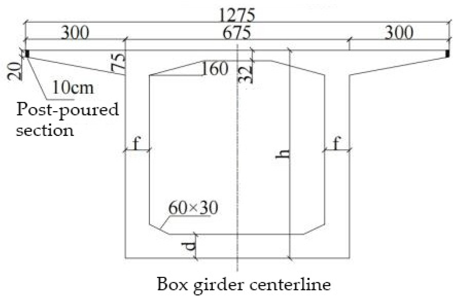
Main Bridge 1# (65 + 5 × 118 + 65 m). The box girder has a depth of 7.0 m at the pier and 2.7 m at midspan, varying along the span following a parabolic law of order 1.8. The top slab width is 12.75 m, the bottom slab width is 6.75 m, and the flange overhang is 3.0 m. The deck provides a transverse crossfall, while the bottom slab is horizontal in the transverse direction.
Main Bridge 2# (76 + 2 × 140 + 76 m). The box girder depth is 8.4 m at the pier and 3.2 m at midspan, also varying along the span following a parabolic law of order 1.8. Piers 26–28 adopt twin-leg rectangular hollow thin-walled sections with a wall thickness of 0.70 m, single-leg thickness of 3.0 m, lateral width 7.75 m, and a clear spacing between legs of 4.0 m. To improve lateral load transfer, the girder–pier junction is widened by 0.5 m on each side, and the foundation uses an integral pile cap. The No.29 transition pier is a rectangular hollow thin-walled section (7.75 m transverse × 5.0 m longitudinal) supported on a separate pile cap (see Figure 3 and Figure 4).
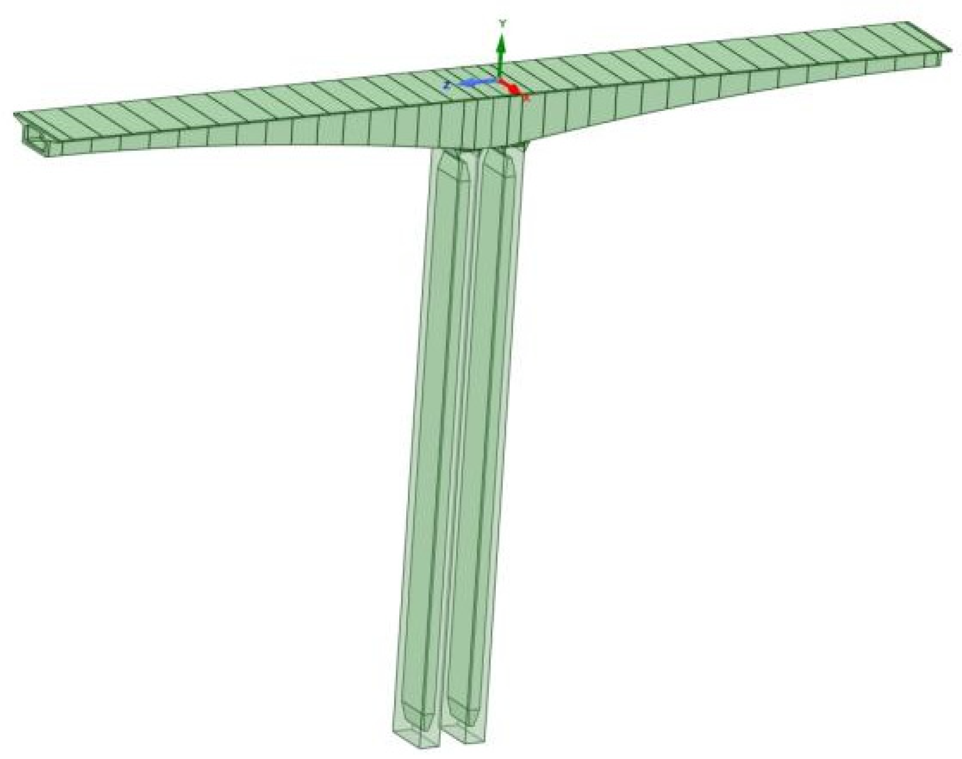
To match the critical construction condition, we select the Main Bridge 2-Pier 26 control unit as the evaluation case (As shown in the dotted box in Figure 3). The girder length of this unit is 145.16 m: on the side-span side, 19 cantilever segments are arranged (closure segment 1.0 m), and on the midspan side, 18 segments are arranged (cast-in-place segment 4.16 m). The girder has a variable depth, with a minimum depth hmin = 3.2 m and a maximum depth hmax = 8.4 m. Based on the above geometry and boundary conditions, a 3D simulation model is established in Ansys Workbench (see Figure 5), and the same reference quantities and coordinate conventions are used consistently in the subsequent finite-element analysis and wind tunnel comparisons.

2.2. Simulation of the Fluctuating Wind Field

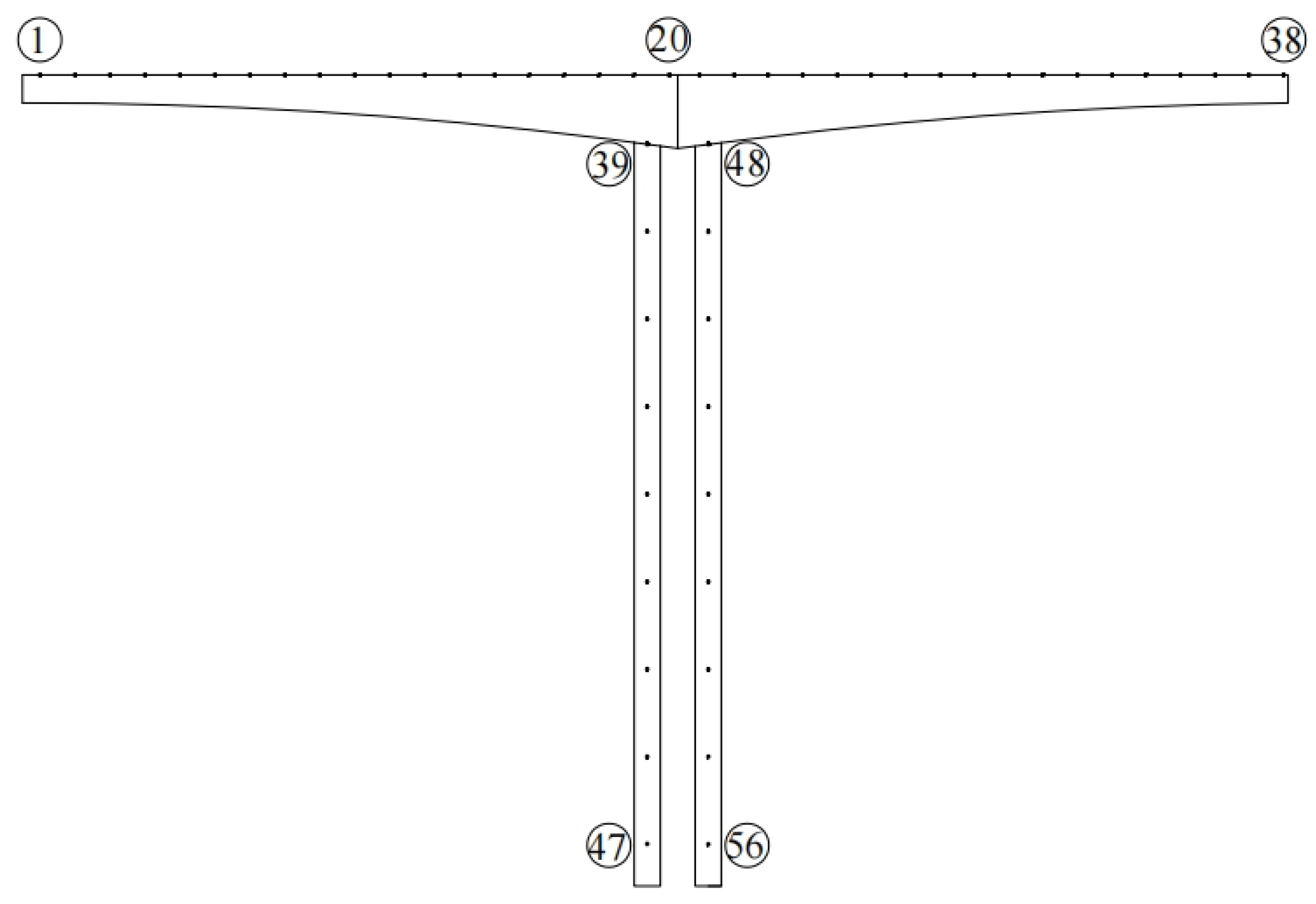
In this study, wind-induced vibration is evaluated using numerically simulated fluctuating wind histories. A site-specific turbulent wind field is built for the Youlian Honghe Bridge, and wind speed time series are generated at multiple locations on the main girder and main pier. Along the girder, 38 points are arranged by construction segment; along the pier, 9 points are placed at equal vertical intervals (Figure 6). The design wind speed is 28 m/s. Fluctuation target spectra follow the Code for Wind-Resistant Design of Highway Bridges [19], and the key simulation parameters are listed in Table 1.
(1)
Target Spectra and Parameters
The fluctuating wind speed spectra are selected in accordance with the Code for Wind-Resistant Design of Highway Bridges (JTG/T 3360-01-2018) [19] (Hereinafter referred to as the “Code”): the along-wind component follows the Kaimal spectrum and the vertical component follows the Panofsky spectrum. The corresponding power spectral density expressions are given in Equations (1) and (2).
Along - wind   ( u ) :   n S u n u * 2 = 200 x 1 + 50 x 5 / 3
Vertical   ( w ) :   n S w n u * 2 = 6 x 1 + 4 x 2
where Su(n) and Sw(n) are the power spectral density functions of the along-wind and vertical components, respectively;
u* is the friction velocity, computed by Equation (3)
u * = k U z ln z z d z 0
where K is the von Kármán constant, taken as K = 0.4;
zd is computed by Equations (2)–(4)
z d = H ¯ z 0 k
where H ¯ is the average height of structures (m); for open, flat terrain zd = 0:
z0 is the surface roughness length; for open, flat terrain zd = 0.05;
f is the Monin coordinate, computed by Equation (5)
f = n z U z
where z is the elevation of the evaluation point;
Uz is the mean wind speed at height z.
(2)
Multi-Point Harmonic Superposition
Harmonic superposition is used in the frequency domain to construct a correlated, multi-point random process. For a one-dimensional, multivariate, zero-mean, stationary Gaussian process, see Equation (6).
f t = f 1 t , f 2 t , , f n t , T
Its cross power spectral density (PSD) matrix is given in Equation (7).
S ( ω ) = s 11 ( ω ) s 12 ( ω ) s 1 n ( ω ) s 21 ( ω ) s 22 ( ω ) s 2 n ( ω ) s n 1 ( ω ) s n 2 ( ω ) s n n ( ω )
Apply the Cholesky decomposition to S(ω); the factor matrix is defined in Equation (9).
f = n z U z
H ( ω ) = H 11 ( ω ) 0 0 H 21 ( ω ) H 22 ( ω ) 0 H n 1 ( ω ) H n 2 ( ω ) H n n ( ω )
To improve efficiency, synthesize the wind speed time histories using FFT [25]:
V j ( t ) = 2 Δ ω m = 1 j l = 1 N H j m ω m l cos ω m l t θ ω m l + ϕ m l
Introducing Euler’s formula e i x = cos x + i sin x , and θ j m ω w l = 0 Equation (10) can be rewritten as Equation (11).
V j t = Re m = 1 j l = 1 N 2 Δ ω H j m ω m l e i ω m l t e i ϕ m l l
After substitution ω m l = ( l 1 ) Δ ω + m n Δ ω , the expression becomes Equation (12).
V j t = Re m = 1 j G j m ( p Δ t ) e i m n Δ ω t
The bracketed term in Equation (12) is exactly the inverse discrete Fourier transform (IDFT); see Equation (13).
G j m = l = 1 N 2 Δ ω e i ϕ m l H j m ω m l e i ( l 1 ) Δ ω t
Let the intermediate quantities be defined as k = l 1 , ( k = 0 , 1 , 2 , , N 1 ) stated B j m = 2 Δ ω e i ϕ m l H j m ω m l , Δ ω = ω N = 2 π f N , then Equation (10) reduces to Equation (14).
G j m ( p Δ t ) = l = 1 N B j m e i k Δ ω t = k = 0 N 1 B j m e i k Δ ω p Δ t
For a signal with longest period T 0 = 2 π Δ ω , sampling interval Δt, and M = T 0 Δ T samples per period, the relations are given by Equations (15) and (16).
T 0 = M Δ t = 2 π Δ ω
Δ t Δ ω = 2 π M
Substituting these into Equations (2)–(14) yields Equations (17) and (18).
G j m ( p Δ t ) = l = 1 N B j m e i k Δ ω t = k = 0 M 1 B j m e i k p 2 x M
B j m = 2 Δ ω e i ϕ m l l H j m ω m l , 0 l < N 0 , N l < M
The IDFT is written in Equation (19).
x ( t ) = 1 N n = 0 N 1 X ( n ) e i 2 π N t n
Therefore, performing the inverse Fourier transform on Bjm enables an efficient synthesis of the wind speed time histories.
(3)
Consistency Check
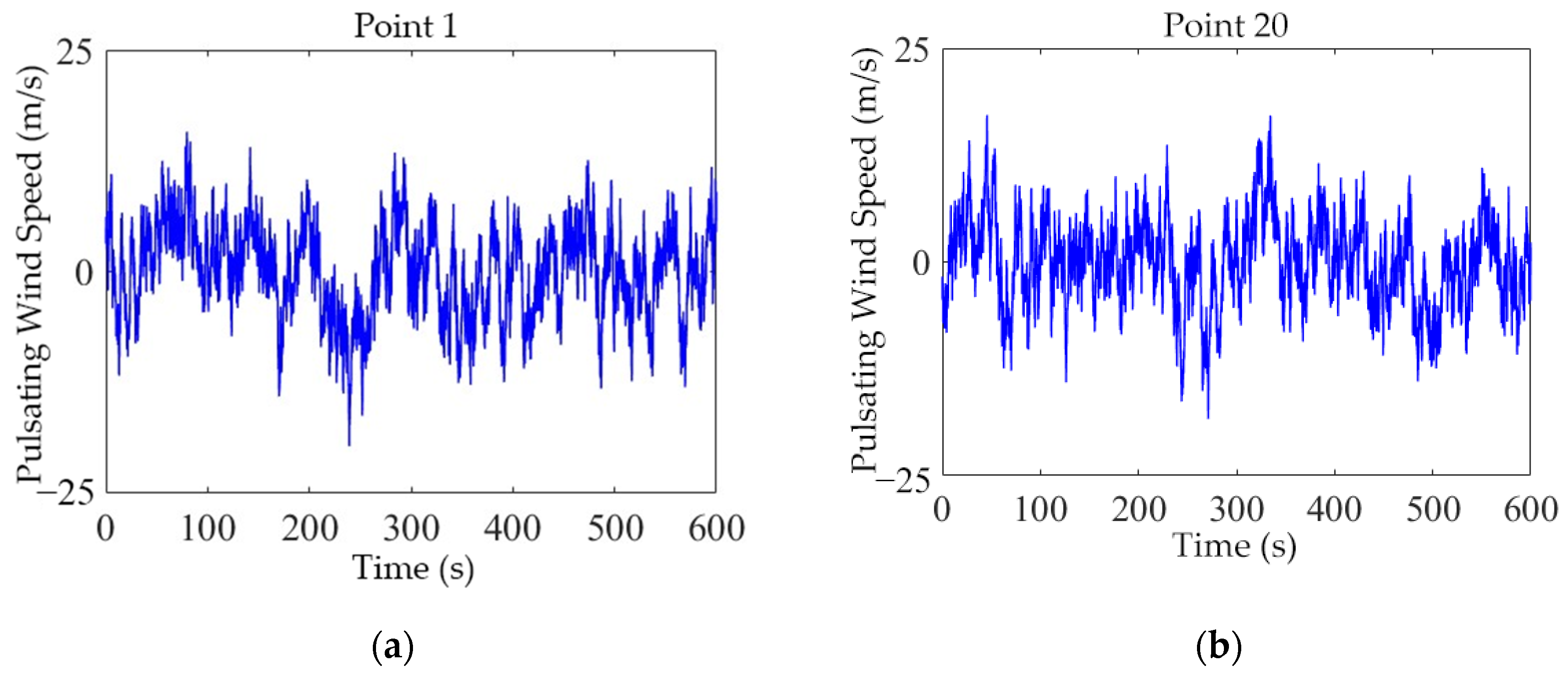
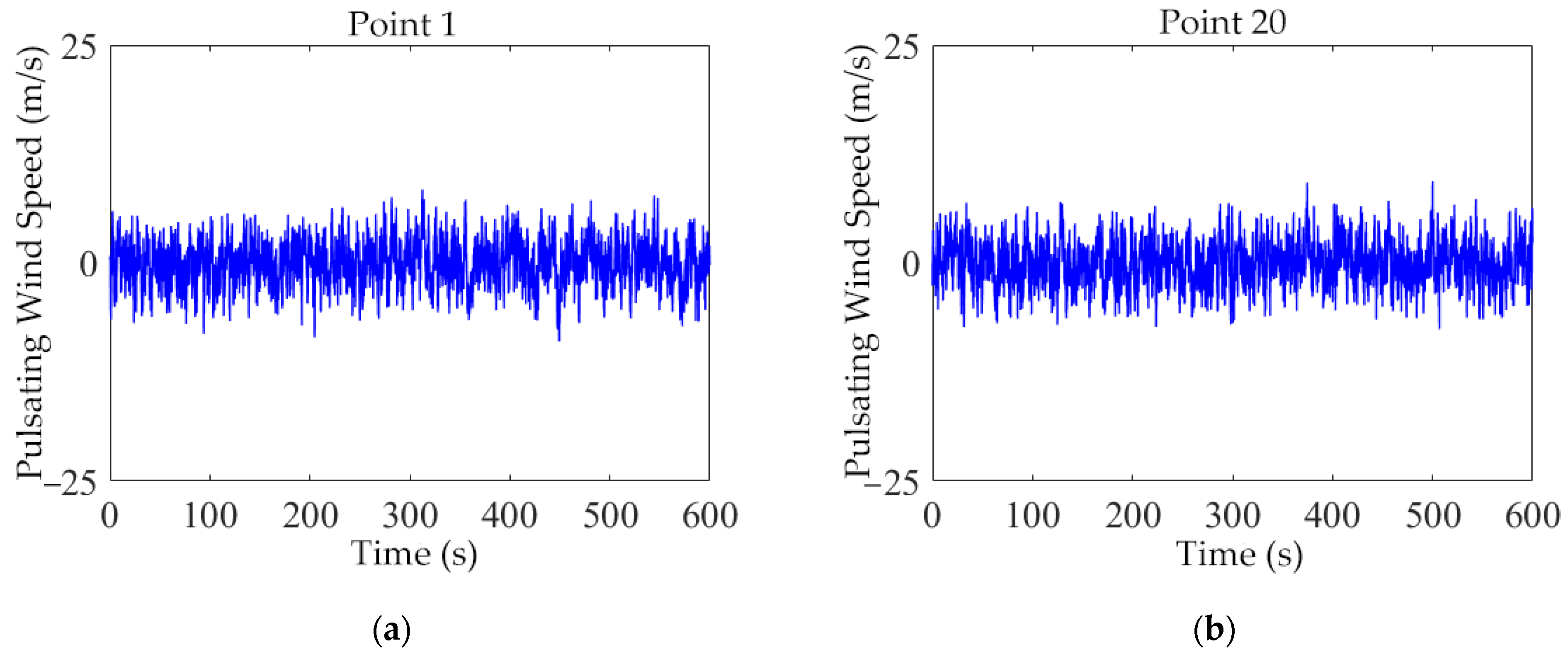
Following the above procedure, the harmonic superposition method is employed, using the Kaimal spectrum for the along-wind component and the Panofsky spectrum for the vertical component. The discrete Fourier transform (DFT) in MATLAB (2023a) is used for spectral conversion, and the FFT is applied to accelerate the transformation from the time to frequency domain. The synthesized fluctuating wind time histories are then generated, and representative time-series plots are provided in Figure 7 and Figure 8 (illustrated for the cantilever tip Point 1 and the midspan Point 20).
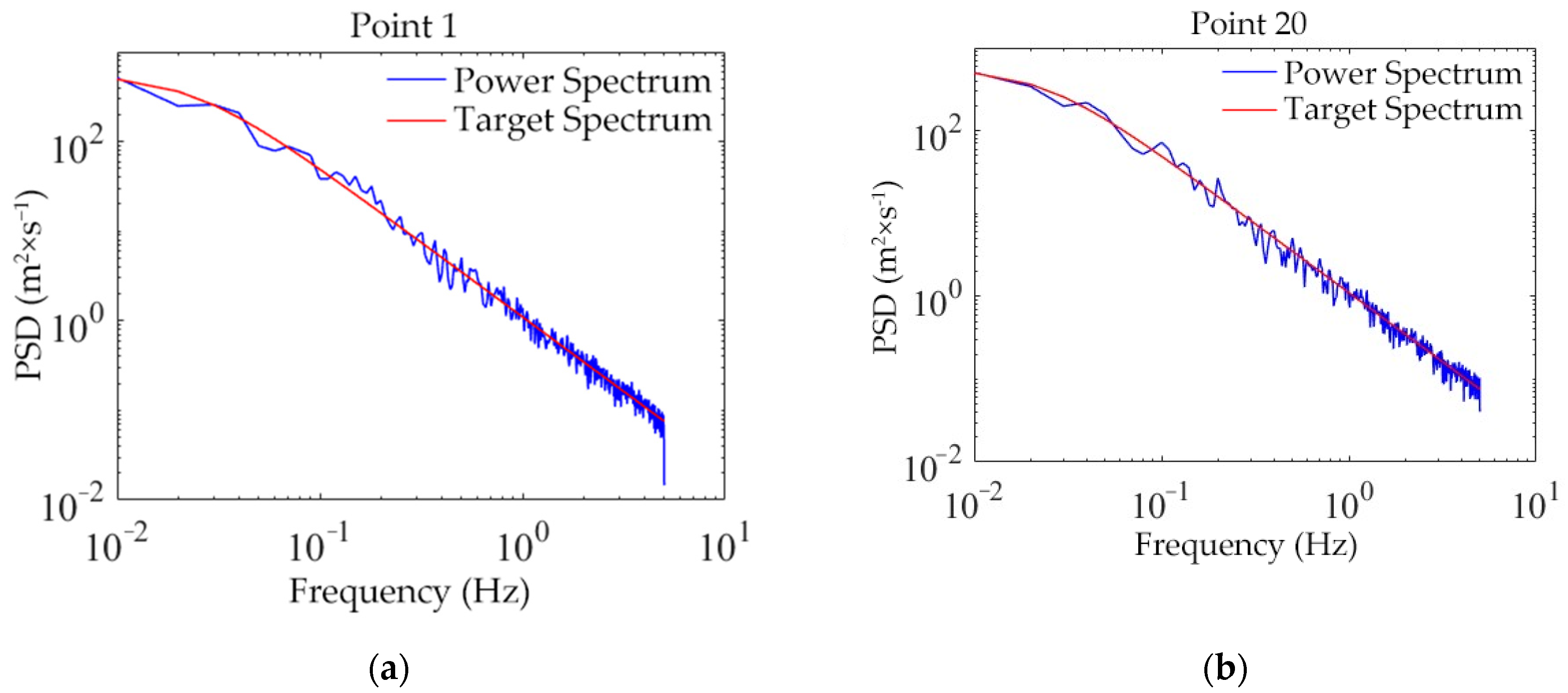
Meanwhile, to validate the simulations, the fluctuating wind PSDs at each measurement point are compared with the target spectra; the fits for Points 1 and 20 are shown in Figure 9 and Figure 10.
From Figure 8 and Figure 9, the PSDs at representative points agree well with the code-based target spectra. Over the main frequency band, the spectral fitting error at each point is <10%, and the standard deviation bias is <5%; the mean square error of coherence curves for typical point pairs is <0.02. Minor deviations appear at the high-frequency end due to finite record length and frequency resolution, but they do not affect the buffeting responses in the 0–2 Hz band considered here. Therefore, the synthesized fluctuating wind can be regarded as a reliable input for the subsequent time-domain analysis.

2.3. Acquisition and Processing of Three-Component Coefficients

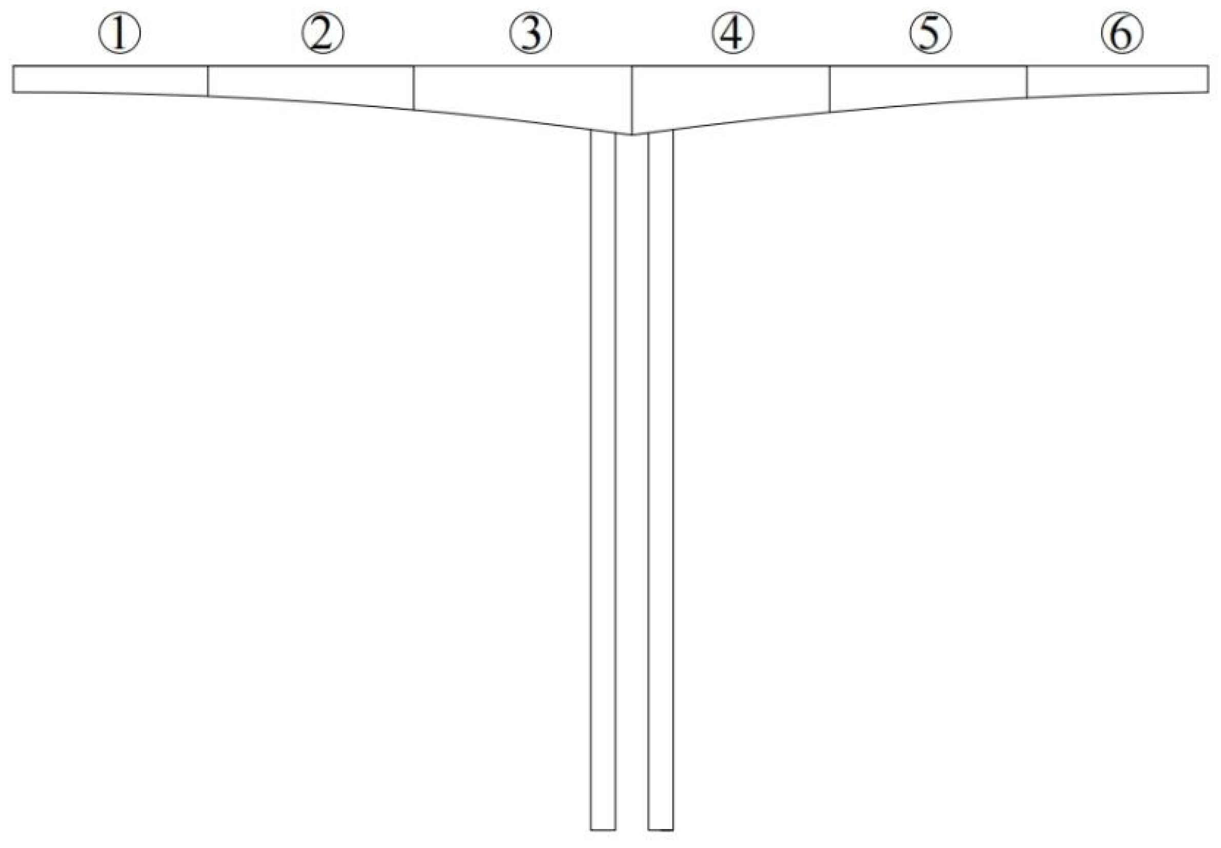
Based on the 3D bridge model established above, the maximum double-cantilever configuration during construction is partitioned into six segments according to the cantilever block layout and computational needs (see Figure 11), yielding segment-wise 3D numerical models. A segmental 3D numerical wind tunnel analysis is then performed in Fluent (steady RANS, standard k-ω model); the inlet turbulence and fluid properties follow Table 2. For 11 angle-of-attack cases within [−10°,10°] increments, we obtain the unit-length static three-component aerodynamic coefficients (in the wind axis system) and their angle-of-attack derivatives. The datasets are subsequently harmonized (coordinate conventions) and functionalized (polynomial fits) to serve as aerodynamic inputs for the downstream time-domain buffeting analysis.
(1)
Computational Domain and Meshing
In three-dimensional external-flow simulations, the computational domain should be large enough that domain-size effects on the solution are minimized. A practical sizing criterion is the blockage ratio. In CFD practice, the blockage ratio is taken as the ratio of the model’s projected frontal area to the cross-sectional area of the flow domain; keeping this ratio small helps maintain stable flow development and numerical accuracy. To mitigate boundary effects, the external domain in this study is therefore sized according to the blockage constraint in Equation (20).
B = A b A d
where Ab is the projected frontal area of the structure;
Ad is the cross-sectional area of the computational domain; the blockage ratio is generally recommended to be ≤3% [26].
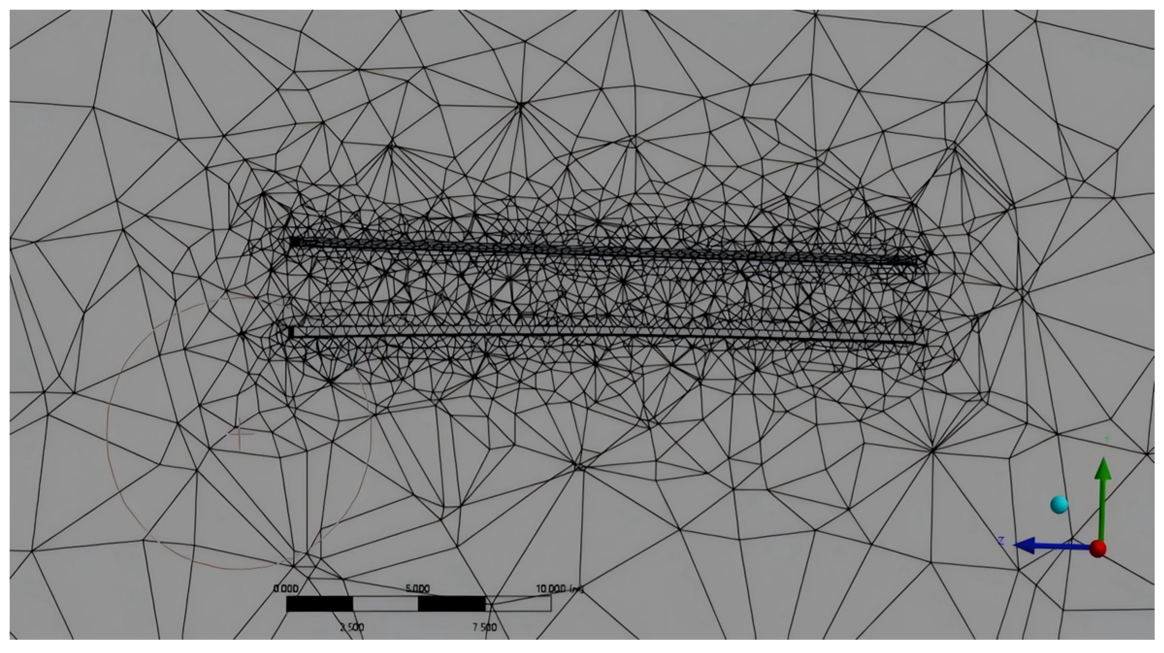
Accordingly, a rectangular external domain is adopted with the inlet 4L upstream of the windward face, the outlet 8L downstream of the leeward face, and the top/bottom boundaries 4H away from the model. The overall domain size is 400 m × 300 m × 80 m, giving a blockage ratio of 2.9%, which satisfies the guideline. Meshing uses near-body refinement around the section (minimum cell size 0.5 m) and coarsening toward the far field (typical cell size 10 m), with smooth size transitions; a local mesh view is shown in Figure 12.
(2)
Three-Component Coefficients for the Main Girder (Construction Stage)
The static three-component coefficients provide a dimensionless characterization of the aerodynamic behavior of a bridge deck under mean wind, corresponding to along-wind drag, vertical lift, and the torsional moment about the deck’s axis. They are key inputs for buffeting, vortex-induced vibration, galloping, and aerostatic stability analyses, and their accuracy directly affects the reliability of wind-resistant assessment [27,28]. In practice, the coefficients are reported in two coordinate systems: the body axis system (FH, FV, FM) and the wind axis system (FD, FL, Mz). Taking the inflow direction as the reference, the wind axis expressions for the static wind loads are given in Equations (21)–(23) [29].
Drag :   F D = 1 2 ρ U 2 C D α D L
Lift :   F L = 1 2 ρ U 2 C L α B L
Torque :   M Z = 1 2 ρ U 2 C M α B 2 L
where CD, CL, and CM are the wind axis drag, lift, and torque coefficients;
ρ is the air density, ρ = 1.225 kg/m3;
U is the incoming wind speed (m/s);
D and B are the girder depth (height) and girder width (m), respectively;
L is the length of the loaded segment (m).
Under the adopted angle-of-attack α convention, the three-component coefficients in the body axis and wind axis systems can be interconverted via a planar rotation.
C H = C D cos α B D C L sin α
C V = D B C D sin α + C L cos α
where CH and CV denote the lateral and vertical force coefficients in the body axis system;
Other symbols are as defined above.
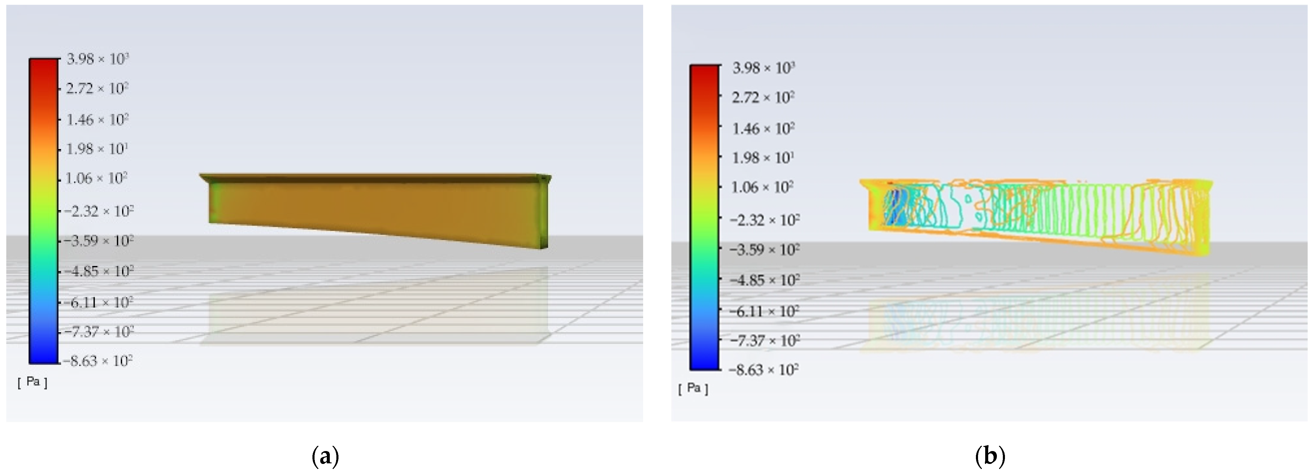
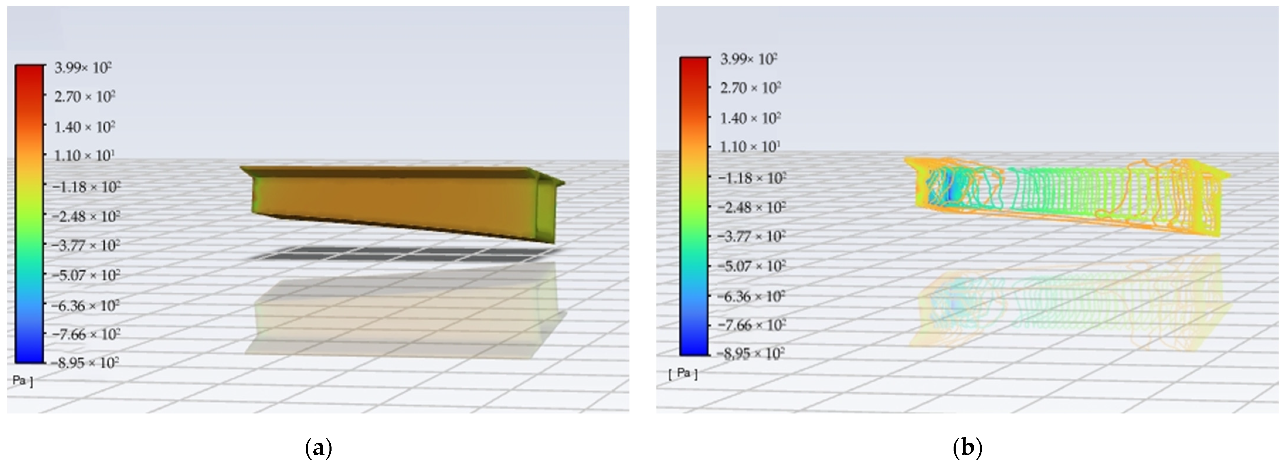
The segmented models are imported into Fluent for three-dimensional external-flow simulations. For each girder segment, computations are performed under 11 angles of attack (α ∈ [−10°,10°], step 2°). For every case, surface pressure contours and streamline plots are produced. Taking Segment 1 as an example, the pressure and streamline fields at α = 0° are shown in Figure 13, and those at α = 10° are shown in Figure 14.

2.4. Time-Domain Buffeting Analysis

2.4.1. Finite-Element Model Setup

The computational model adopts the following assumptions to ensure reasonable and reproducible results. Firstly, the wind field is simulated under the quasi-steady assumption; within each time step the wind speed varies slowly so that the instantaneous aerodynamic force can be approximated as steady. The aerodynamic excitation follows the von Kármán turbulence spectrum, consistent with the construction-stage wind environment of high-pier, long-span continuous rigid-frame bridges. Structural damping is treated in a modal manner, with damping ratios for each mode taken from the relevant code recommendations. Time integration uses a step size of Δt = 0.02 s and a total simulated duration of T = 600 s, sufficient for buffeting responses to develop. During the solution process, the finite-element convergence tolerance is set to 1 × 10⁻⁵ to ensure numerical accuracy and stability. These assumptions provide a consistent basis for the subsequent buffeting analysis and help maintain self-consistency across all steps.
Building on the above assumptions, an APDL-based finite-element (FE) model is established for the maximum double-cantilever configuration of the Youlian Honghe Bridge (Main Bridge, Pier 26).
The BEAM188 element [24] is used for both the main girder and the main pier, with KEYOPT(1) = 0, which means there are six degrees of freedom per node (translations along x,y,z and rotations about x,y,z). Rigid connections at the girder–pier interface and the pier–foundation fixity are modeled using MPC184 elements, which implement multi-point constraints via Lagrange multipliers and can output constraint forces and moments; they are therefore suitable for representing rigid load transfer between deformable bodies and boundary fixities.
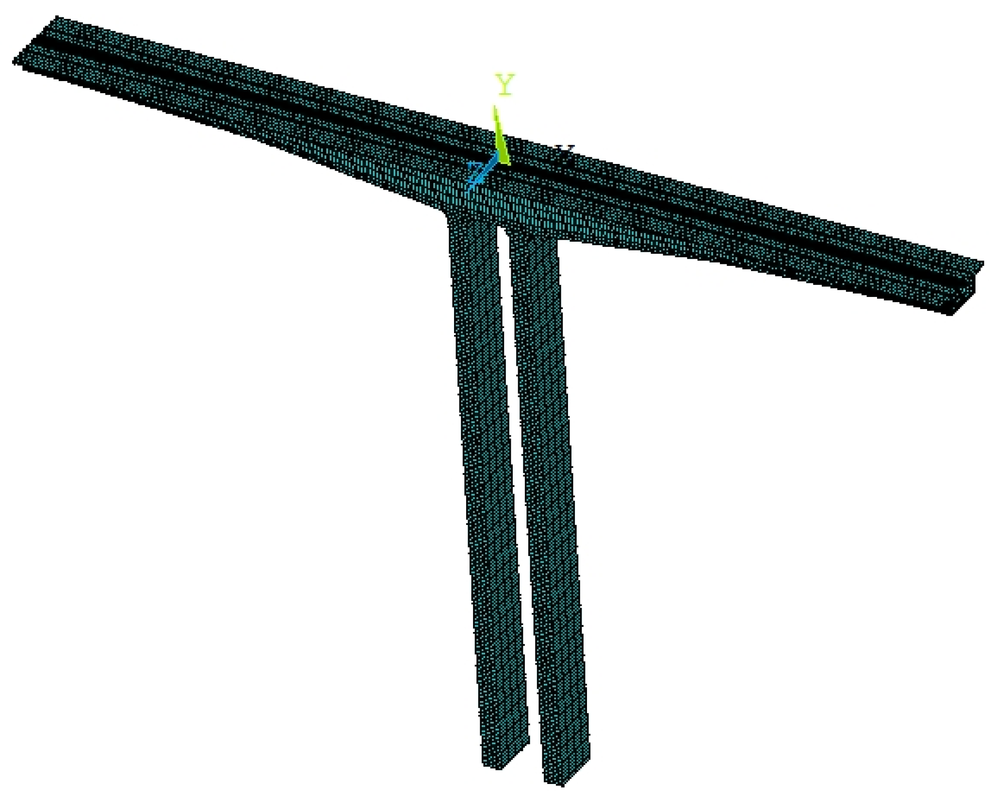
Material properties follow the engineering design: C55 concrete for the main girder and C50 concrete for the main pier. The model comprises 680 elements and 1663 nodes. The mechanical parameters are listed in Table 3, and the overall FE model of the maximum double-cantilever T-type configuration is shown in Figure 15.

2.4.2. Aerostatic (Static Wind) Stability Analysis

Aerostatic stability shows strong load–deformation coupling: under the mean wind, the main girder bends and twists, shifting the effective angle of attack and thereby changing the static three-component coefficients, which in turn modifies the external loads. Accordingly, we first compute static wind loads using code formulas, then iteratively update the deformed configuration—angle of attack, aerodynamic coefficients, and loads—until convergence. This deformation-updated loading provides the applied values on the girder and yields a more accurate assessment of aerostatic stability [30].
(1)
Calculation of Aerostatic (Static Wind) Loads
The design reference wind speed at the bridge reference height Z is obtained from Equation (4.2.6-1) of the Code [19]:
U d = k f Z 10 α 0 U S 10 = 39.23   m / s
where kf is wind resistance risk factor, kf = 1.02 per Table 4.2.6-1 of the Code [19];
α0 is the ground roughness coefficient at the bridge site, according to Table 4.2.1 in the Code [19], α0 = 0.16 is retrieved.
The construction-stage design wind speed is then determined using Equation (4.2.9) in the Code [19]:
U s d = k sf U d = 34.52   m / s
where ksf is the construction-stage wind resistance risk factor; ksf = 0.88.
According to the design drawings, the elevation of each cantilever block (center height above ground) is identified from the deck and ground levels. Using these heights, the equivalent static gust wind speed for the construction stage is evaluated via Equation (5.2.1) in the Code [19]:
U g = G v U d
where Gv is the equivalent static gust factor, taken from Table 5.2.1 of the Code [19].
Following the above procedure, the equivalent static gust wind speeds for all construction blocks of the Youlian Honghe main bridge during the construction stage are summarized in Table 4.
(2)
Aerostatic Stability Analysis
A geometrically nonlinear analysis with load increments and inner–outer iterations is adopted. Using ANSYS (2023 R1) APDL secondary development, a command stream is written for the aerostatic stability procedure. The implementation steps are as follows [31]:
(1)
Perform a nonlinear solution under self-weight (stepi−1 = step0).
(2)
Extract the torsional angle vector of the main girder {θ}i−1, and compute the corresponding three-component coefficients; at this stage the effective angle of attack equals the initial value α0.
(3)
Prescribe an initial wind speed U0 and an increment ΔU; set the current wind speed Ui = U0(stepi).
(4)
At Ui, solve the geometric and material nonlinearity using the Newton–Raphson method to obtain a converged solution (inner iteration).
(5)
Extract the updated torsional angle vector of the (stiffened) main girder {θ}i, and recompute the three-component coefficients for this deformed state.
(6)
Check whether the Euclidean norm of the change in three-component coefficients is below the tolerance:
j = 1 N a C k α j C k α j 1 2 j = 1 N a C k α j 1 2 1 2 e p s k k = X , Y , Z
where Na is the total number of nodes;
Ck denotes the drag, lift, or torsional moment coefficient;
i is the current load step index;
epsk is the tolerance for the drag, lift, and torsional moment coefficients, taken as 5 × 10⁻⁷.
(7)
If the norm exceeds the tolerance, repeat steps (4)–(6) (outer iteration). If the number of iterations exceeds the preset limit, the current wind speed level is deemed difficult to converge; halve the wind speed increment and return to step (4) to recompute. If the increment falls below the preset minimum, terminate the analysis.
(8)
If the norm is within the tolerance, the solution at the current wind speed is converged; output the results and increase the wind speed by the specified increment to proceed to the next level.
(9)
Plot the deformation–wind speed curves and determine the critical wind speed for aerostatic instability.
Previous studies indicate that, under static wind loads, the displacement distribution along long-span bridges is non-uniform, with the cantilever tip often governing. Accordingly, the right cantilever tip of the main girder is selected as the representative point to establish the displacement–wind speed relationship (see Figure 16).
From Figure 16, at the test wind speed of 28 m/s, the lateral, vertical, and torsional responses are 0.185 m, −0.134 m, and −0.003 rad, respectively. At the design wind speed of 34.52 m/s, the midspan increments in all three directions are close to zero, indicating a relatively stable state. With further increases in wind speed, the responses grow markedly, and the aerostatic critical wind speed is about 140 m/s, which exceeds both the project background wind and the historical extreme (instantaneous wind speed of about 113 m/s at Barrow Island in 1996). This suggests ample safety margin in terms of aerostatic stability and supports the validity of the FE model and the adopted analysis workflow.

2.4.3. Dynamic Characteristics

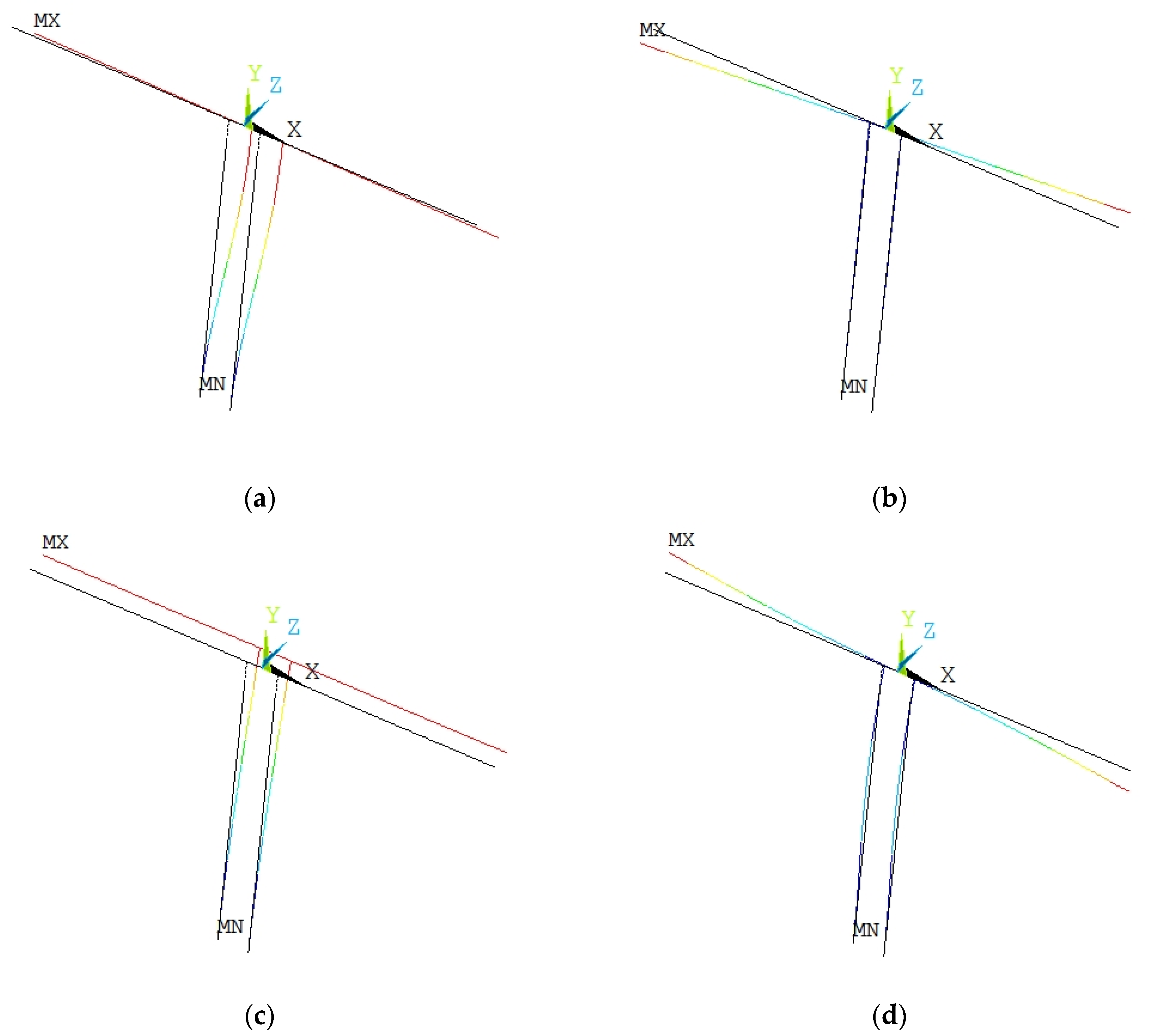
A modal analysis is performed on the FE model under the maximum double-cantilever condition. The first ten natural frequencies and mode descriptions are summarized in Table 5. The first three modes are governed by pier bending and torsion; mid- to high-order modes are dominated by girder vertical and lateral bending. Representative mode shapes are illustrated in Figure 17 (Black and white means before the deformation, color means after the deformation).
From Table 5 and Figure 17, the first three natural frequencies are approximately 0.189 Hz, 0.212 Hz, and 0.261 Hz, corresponding to pier bending (longitudinal), pier torsion, and pier bending (lateral), respectively; these constitute the dominant low-frequency modes relevant to subsequent buffeting. Mid- to high-order modes are mainly governed by girder vertical and lateral bending (about 0.764–2.72 Hz) with some coupling to pier bending. This spectral distribution is consistent with the 0–2 Hz band emphasized in the synthesized turbulent wind field, providing a modal basis for the analysis of response peaks and time–frequency characteristics.

2.4.4. Buffeting Response Analysis

A time-domain approach is adopted for the buffeting analysis. Under the quasi-steady assumption, the multi-point fluctuating wind synthesized and validated in Section 2.2 is combined with the three-component aerodynamic coefficients and their angle-of-attack derivatives obtained in Section 2.3. Following the Davenport model (see Equations (30)–(32)), the segment-wise time histories of the buffeting drag, lift, and torsional moment are computed.
D b t = 1 2 ρ U 2 B 2 C D α χ D u A B u x , t U + C D α χ D w w x , t U
L b t = 1 2 ρ U 2 B 2 C L α χ L u u x , t U + C L α + A B C D α χ L w w x , t U
M b t = 1 2 ρ U 2 B 2 2 C M α χ M u u x , t U + C M α χ M w w x , t U
where Db, Lb, and Mb are the buffeting drag, lift, and torsional moment in the wind axis system;
α is the angle of attack;
ρ is the air density (taken as 1.225 kg/m3);
B is the reference girder width;
U is the design reference wind speed (28 m/s);
CD, CL, and CM are the drag, lift, and torque coefficients;
CD′, CL′, and CM′ are their derivatives with respect to α;
u(t) and w(t) are the along-wind and vertical fluctuating wind components;
AD and AL are the projected areas in the lateral and vertical directions;
χkl (k = D, L, M; l = w, u) denotes the aerodynamic admittance. In this study, admittance corrections are not applied and all χkl are set to 1.
The segment-wise line loads Db(t), Lb(t), and Mb(t) are mapped to equivalent nodal forces and moments in the FE model using a consistent loading scheme, then superimposed on the aerostatic baseline and integrated in time by direct transient analysis (time step consistent with the wind field sampling). The reported outputs include RMS and peak responses and the buffeting amplification factors relative to the static wind results, which are subsequently compared with the wind tunnel measurements.

2.5. Six-Component Wind Tunnel Tests (Benchmark)

(1)
Similarity Criteria and Inflow Conditions
The tests were conducted in the Boundary-Layer Wind Tunnel of Northeast Forestry University. The test section measures approximately 1.0 m (H) × 0.8 m (W) × 5.0 m (L). The inflow is driven by a continuously variable DC motor, with a maximum wind speed of about 70.5 m/s. A honeycomb straightener is installed upstream of the test section; the flow quality satisfies the requirements for static force measurements, with turbulence intensity ≤ 0.5% and velocity uniformity Δv/v ≤ 0.5%. A full-bridge rigid model was manufactured following geometric similarity. The blockage ratio of the test section is kept <10%; when it exceeds 5%, a blockage correction is applied according to the standard formula. The blockage ratio γ is computed as in Equation (33) [32].
γ = A m A c
where Am is the cross-sectional area of the wind tunnel test section (m2);
Ac is the sum of the maximum projected areas of the test model and any fixtures within the tunnel (m2).
The computed blockage ratio is 3.6%, which is <5%, satisfying the code requirement.
(2)
Test Model and Measurement System
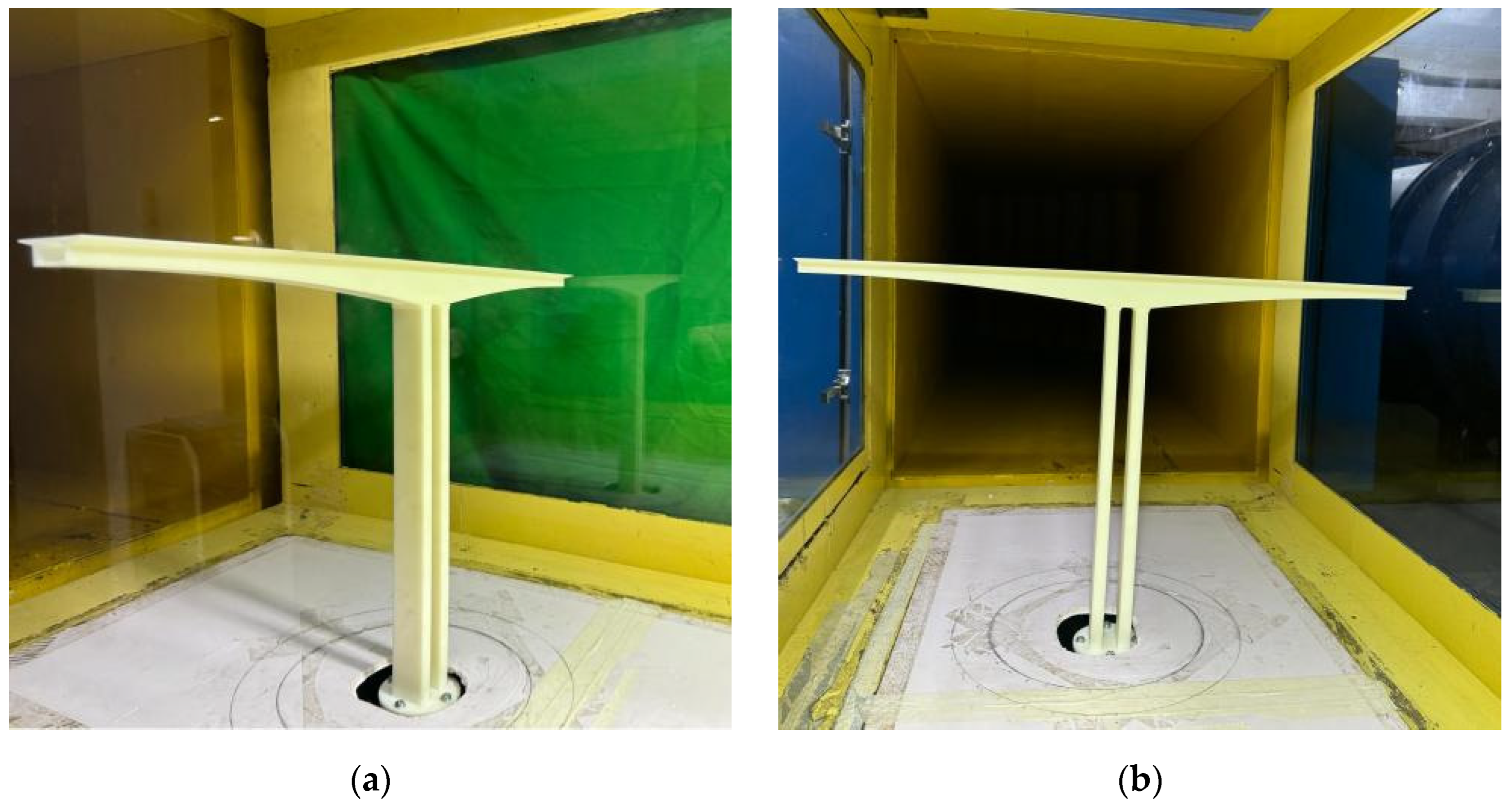
A full-bridge model was fabricated from PLA (polylactic acid) using 3D printing at a geometric scale of 1:180 (see Figure 18). A strain gauge six-component force balance served as the measurement system. The balance—comprising an elastic body, bonded foil strain gauges, and a measurement circuit—simultaneously records the three forces and three moments acting on the model in the body axis coordinate system. During testing, the aerodynamic loads on the model are transmitted through the support to the balance, producing minute elastic deformations; the associated strains change the gauge resistance and generate a bridge circuit voltage proportional to the external load. After amplification and calibration, the voltage signals are fed into a computer to obtain the static six-component data (force, moment time histories and their means), which are then used for coefficient evaluation and subsequent comparison analyses.
Given that the bridge model is a three-dimensional spatial structure, static three-component coefficients alone cannot fully characterize its aerostatic behavior [33]. To capture the wind-loading mechanism beyond the strip assumption, a static six-component test is therefore adopted. In the body axis coordinate system, the physical definitions and calculation formulas of the six components are given by Equations (34)–(39):
Lateral   force :   F X = 1 2 ρ U 2 C X α D
Vertical   force :   F Y = 1 2 ρ U 2 C Y α B
Longitudinal   ( streamwise )   force :   F Z = 1 2 ρ U 2 C Z α B
Yawing   moment   ( about   the   vertical   axis ) :   M X = 1 2 ρ U 2 C M X α D 2
Rolling   moment   ( about   the   longitudinal   axis ) :   M Y = 1 2 ρ U 2 C M Y α B 2
Pitching   moment   ( about   the   lateral   axis ) :   M Z = 1 2 ρ U 2 C M Z α B 2
In the wind axis coordinate system, the static six components are computed by Equations (40)–(45):
Drag :   F D = 1 2 ρ U 2 C D α D
Lift :   F L = 1 2 ρ U 2 C L α B
Side   ( lateral )   force :   F O = 1 2 ρ U 2 C O α B
Rolling   moment   ( about   the   streamwise   axis ) :   M D = 1 2 ρ U 2 C M D α D 2
Yawing   moment   ( about   the   vertical   axis ) :   M L = 1 2 ρ U 2 C M L α B 2
Pitching   moment   ( about   the   lateral   axis ) :   M O = 1 2 ρ U 2 C M O α B 2
where CX, CY, CZ, CMX, CMY, and CMZ denote the unit-length coefficients in the body axis system for the lateral force, vertical force, streamwise (longitudinal) force, yawing moment, rolling moment, and pitching moment, respectively;
CD, CL, CO, CMD, CML, and CMO denote the corresponding unit-length coefficients in the wind axis system for the drag, lift, side force, rolling moment, yawing moment, and pitching moment, respectively;
α is the angle of attack (deg);
ρ = 1.225 kg/m3 is the air density;
U is the incoming wind speed (m/s);
D and B are the girder depth (height) and girder width (m).
Following the conversion relations given in current codes for three-component coefficients between the body axis and wind axis systems, the six-component conversion relations are derived by analogy, as presented in Equations (46)–(51).
C X = C D cos α B D C L sin α
C Y = C O cos α
C Z = D B C D sin α + C L cos α
C MX = C M D cos α B D C ML sin α
C MY = C M O cos α
C M Z = D B C M D sin α + C M L cos α
(3)
Test Conditions and Procedure
The baseline inflow speed was set to 28 m/s, with a 30 s sampling duration per case. The angle of attack ranged from −10° to 10° in 2° increments (11 cases). A strain gauge six-component balance measured the static forces and moments on the model; after coordinate transformation, the results were expressed in the wind axis system. The data were then processed using an in-house MATLAB script to obtain the static six-component coefficients of the full-bridge model (wind axis) at each angle of attack, which were subsequently compared with the numerically derived three-component results.

3. Results and Discussion

3.1. Three-Dimensional Numerical Simulation: Results and Analysis

3.1.1. Static Three-Component Coefficients

Based on the segmental 3D numerical wind tunnel analysis (Section 2.3), wind axis three-component coefficients were obtained for six representative segments under 11 angles of attack (α = ±10°, ±8°, ±6°, ±4°, ±2°, 0°). For brevity, only the results for α = −2°, 0°, 2° are reported here; the statistics for each segment are summarized in Table 6.
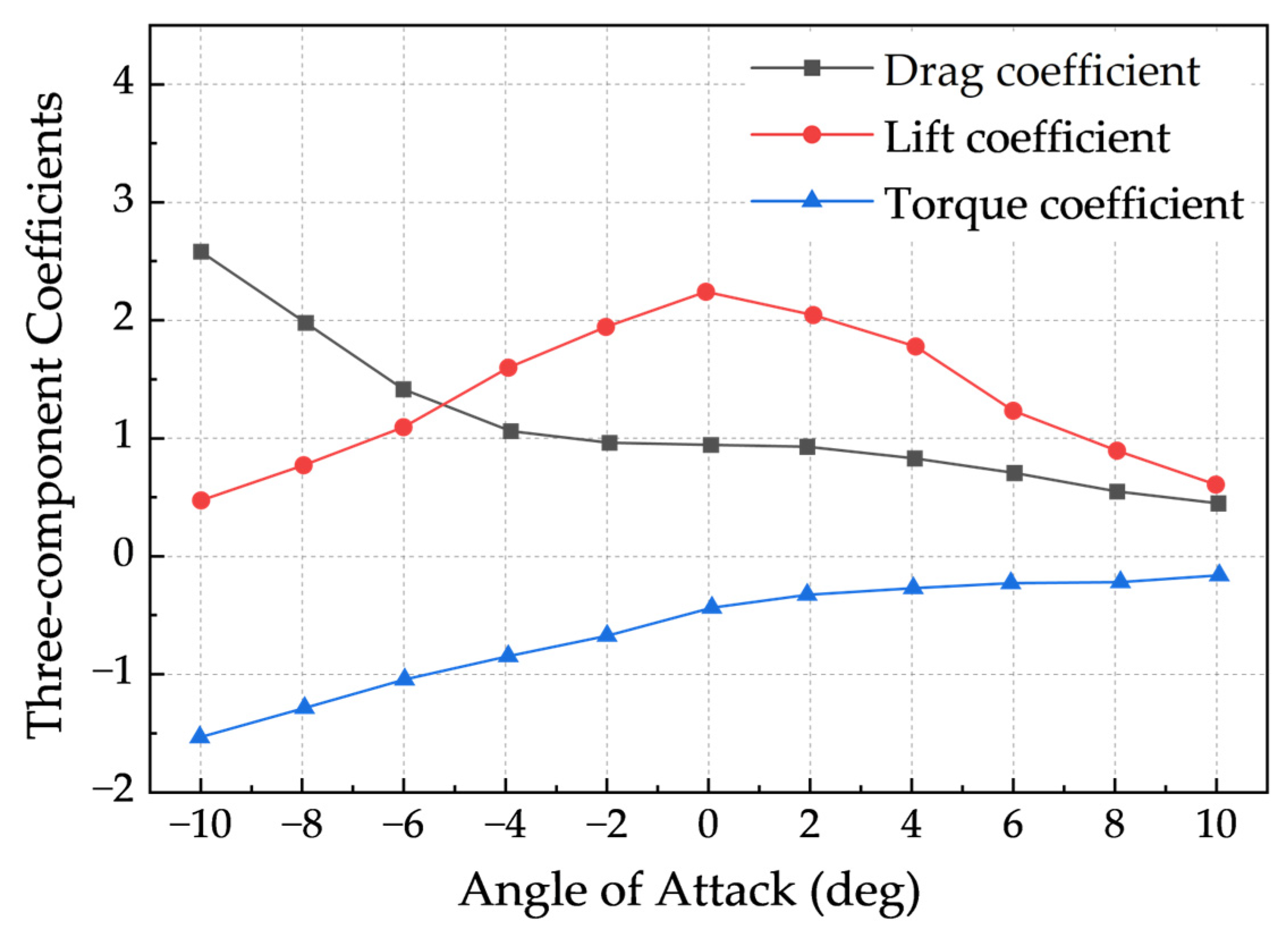
The variation in the static three-component coefficients with the angle of attack for Segments 1 and 3 is shown in Figure 19 and Figure 20.
From the figures, within a given segment, the lift coefficient is most sensitive to the angle of attack, whereas the torsional moment coefficient shows the weakest dependence. Moving toward midspan, the girder geometry becomes more uniform, the flow is steadier with lower turbulence intensity, and the three-component coefficients exhibit reduced sensitivity to the angle of attack, highlighting the differing angle of attack sensitivity caused by the variable depth and boundary effects.
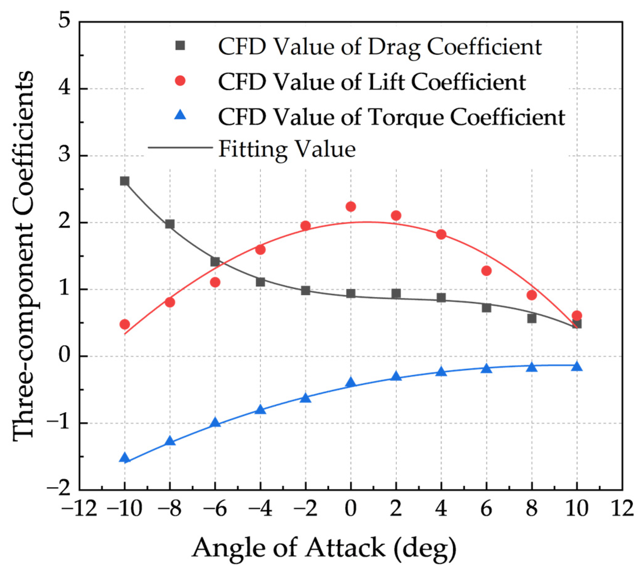
For direct use in the time-domain analysis, the coefficient–angle of attack relationships are functionalized via polynomial fits. Taking Segment 1 as an example, the fitted expressions for CD(α), CL(α), and CM(α) are given in Equations (52)–(54).
The corresponding fitted curves are shown in Figure 21.
C D = 0.00082389 x 3 + 0.00618 x 2 0.02698 x + 0.89974
C L = 0.000188634 x 3 0.01615 x 2 + 0.02353 x + 2.00076
C M = 0.00003213 x 3 0.00403 x 2 + 0.07075 x 0.45140
From Figure 21, the fitted curves match the CFD data well and capture the overall trends of the three-component coefficients. The drag coefficient CD decreases with the increasing α, with a notable drop over −8°~2° and a milder slope beyond 4°. The lift coefficient CL follows a downward-opening parabola, peaking near 2°~4°; outside this region it increases with α for negative angles and decreases with α for positive angles. The torsional moment coefficient CM grows approximately monotonically with α, indicating a higher sensitivity of the pitching moment to the angle of attack. Overall, end segments (Segment 1) show larger magnitudes and steeper slopes with respect to α than midspan segments, reflecting the stronger angle-of-attack sensitivity induced by the variable depth and boundary effects. Around small positive α, the combined action of the lift and pitching moment is more likely to amplify the vertical and torsional responses in subsequent buffeting analysis.
For time-domain use, the fitted coefficient–angle of attack relations are differentiated to obtain CD′(α), CL′(α), and CM′(α) (Equations (55)–(57)). Representative derivative values at α = −2°, 0°, 2° are summarized in Table 7. These derivatives serve as aerodynamic inputs to the Davenport quasi-steady model for buffeting force synthesis.
C D = 0.00494334 x + 0.02472
C L = 0.001131804 x 0.0646
C M = 0.00019278 x 0.01612

3.1.2. Buffeting Response

(1)
Buffeting Force Time Histories
Using the synthesized fluctuating wind records (Section 2.2) together with the static three-component coefficients and their angle-of-attack derivatives (Section 3.1.1), the Davenport quasi-steady model (Equations (27)–(29)) is applied to compute segment-wise buffeting line loads, which are then mapped to equivalent nodal forces and moments in the FE model. The resulting time histories of the drag, lift, and torsional moment at representative nodes are obtained; an example for Node 20 is shown in Figure 22.
From Figure 22, the three directional force time histories fluctuate about zero with nearly constant amplitude over the entire record, indicating stationary random processes. The torsional moment exhibits the largest fluctuations—on the order of 105 (in the model’s SI units)—and shows a slight negative bias under small positive angles of attack, suggesting a higher sensitivity of torque to α. The drag and lift display smaller amplitudes. The amplitude ranking of the three components is approximately M b > D b > L b . Power is primarily concentrated in the 0–2 Hz main frequency band, providing the driving input for subsequent response analysis.
(2)
Time-Domain Buffeting Analysis
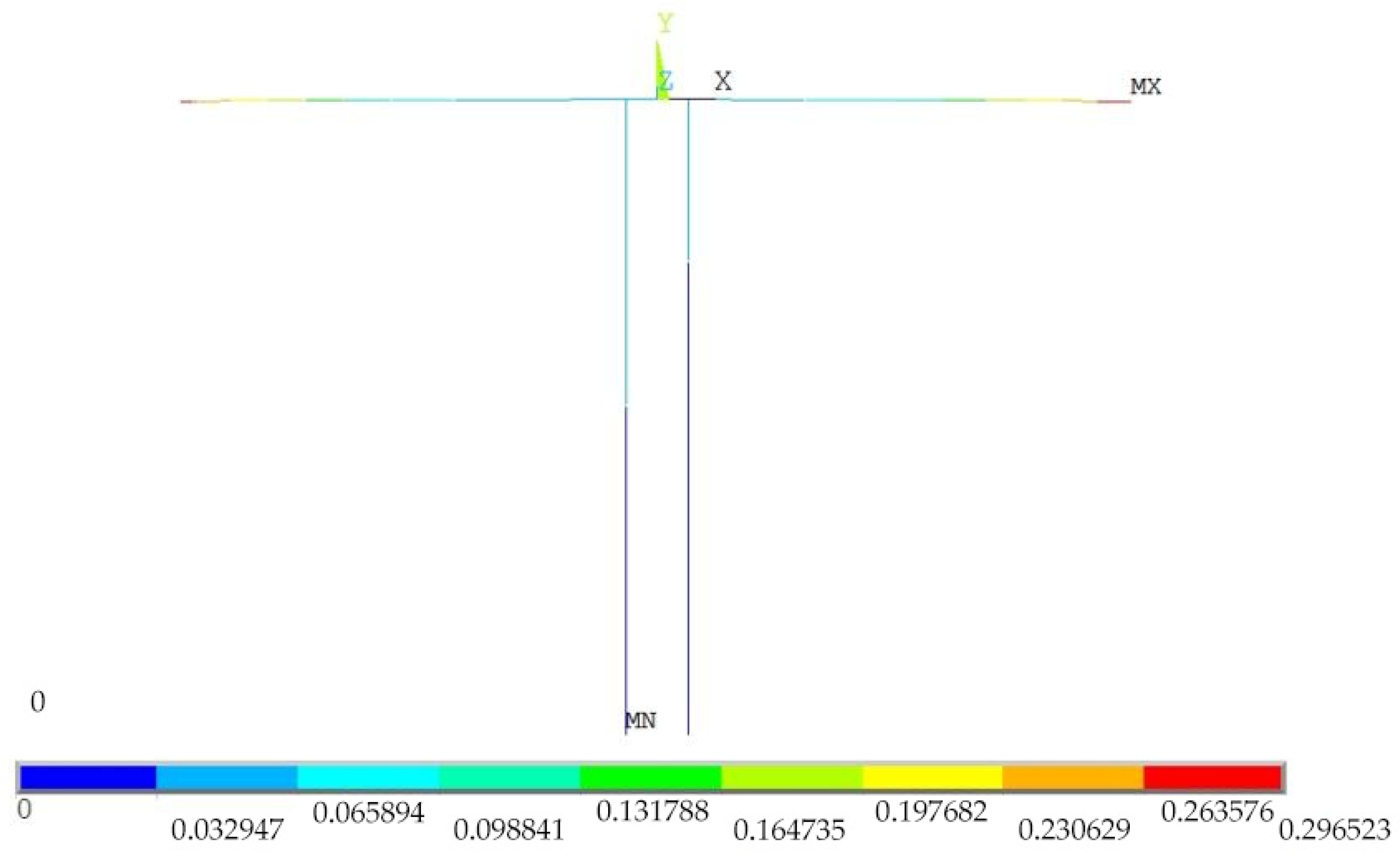
The three-direction buffeting line loads from Equations (27)–(29) are converted to equivalent nodal forces and moments in the APDL FE model. A 600 s loading duration is used, and the maximum double-cantilever configuration is integrated with a linear direct transient scheme. Figure 23 shows the load locations; Figure 24 presents the global deformation pattern.
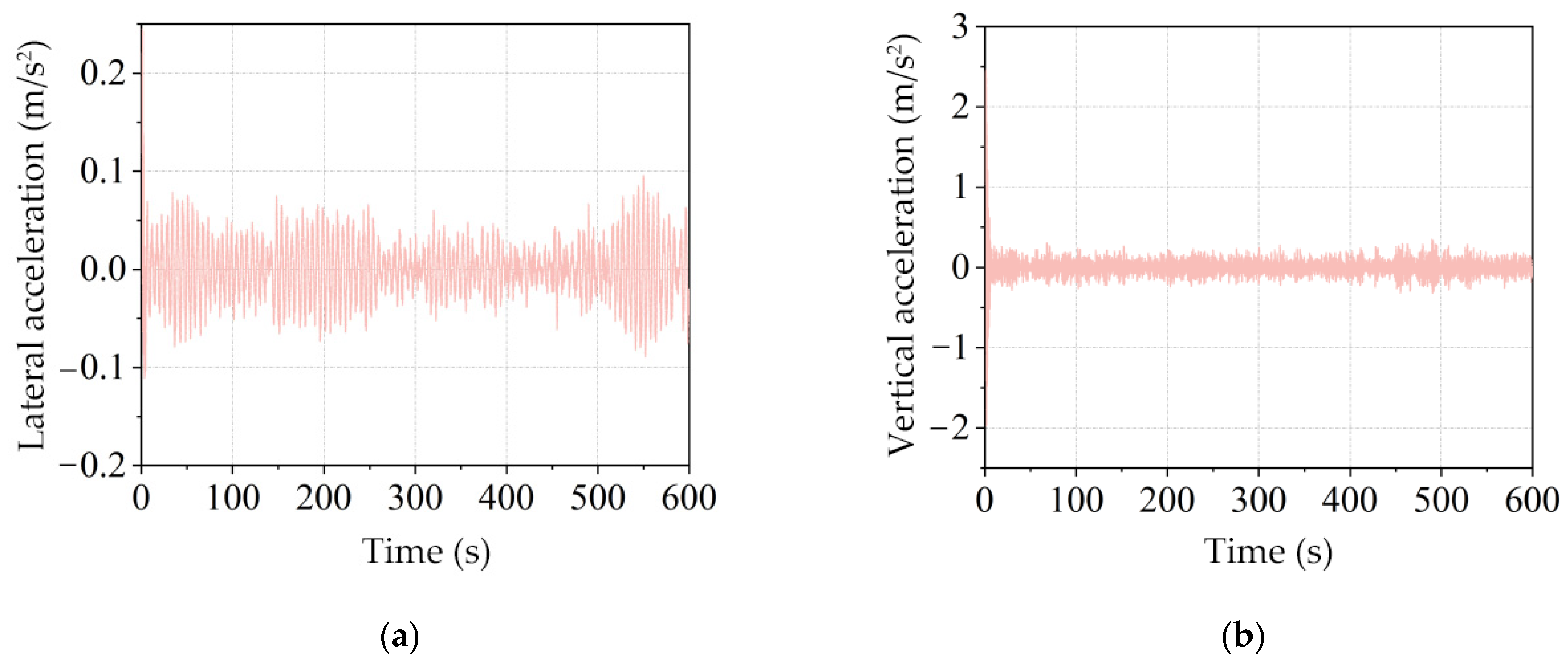
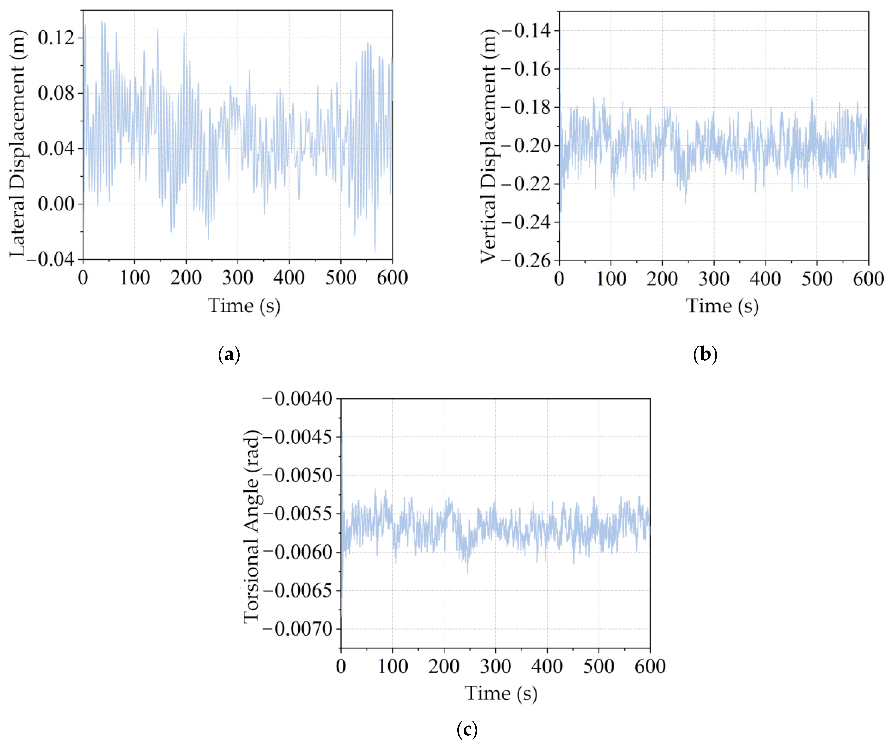
At the right cantilever tip, the acceleration and displacement and torsional angle time histories (Figure 25 and Figure 26) exhibit zero mean and nearly stationary variance. The response energy is concentrated in the first low-frequency band (0.19–0.26 Hz) consistent with the dominant pier modes. Among the three components, the torsional response shows the largest fluctuations, indicating a higher sensitivity to the fluctuating lift and pitching moment inputs.
As shown in Figure 27, the along-span RMS displacements are larger at the cantilever ends and smaller at midspan for both the lateral and vertical components; the torsional RMS likewise reaches its maximum at the ends. This distribution is consistent with the variable-depth configuration and the end-restraint conditions.
Further comparing the static peak and the buffeting peak at 28 m/s (Table 8), the buffeting amplification factors at the right cantilever tip are 1.88 (lateral), 2.75 (vertical), and 3.10 (torsion). This indicates that torsional response is most susceptible to amplification, followed by vertical, with lateral being relatively less affected.

3.2. Wind Tunnel Results and Analysis

3.2.1. Static Six-Component Coefficients

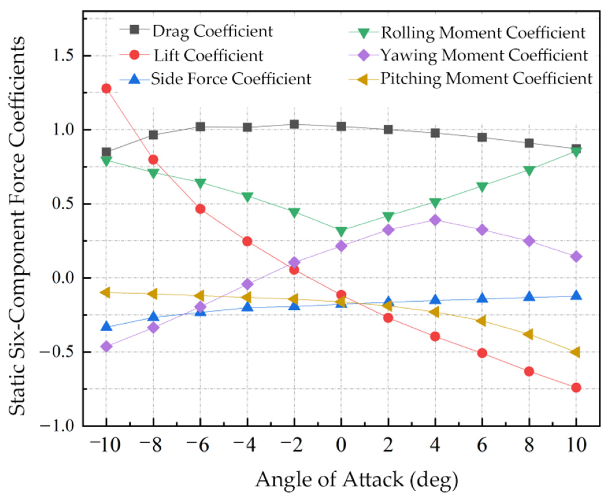
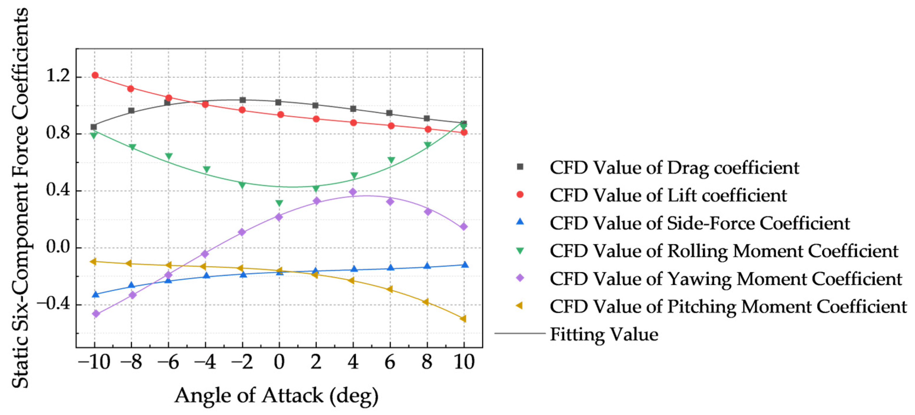
Static six-component tests were conducted at the baseline wind speed U = 28 m/s over an angle-of-attack range α = −10° to +10°. The raw balance measurements were first recorded in the body axis system (three forces and three moments) and then transformed to the wind axis system to obtain the corresponding six-component coefficients. The measured results at each angle of attack are summarized in Table 9, and the overall trends with α are shown in Figure 28.
From the test results, the drag coefficient attains a larger value near small negative angles of attack and then decreases slowly as α increases; the lift coefficient increases and then decreases as α varies from negative to positive, peaking at a small positive angle; the side force coefficient increases monotonically with α (rising from negative toward zero); the rolling moment coefficient exhibits a “U”-shaped trend and is sensitive to small positive α; the yawing moment coefficient generally increases with α with a slight drop at larger positive angles; and the pitching moment coefficient decreases approximately monotonically with α. Compared with the three-component results, these features further reveal the influence of force–moment coupling in the small α range. For subsequent time-domain analysis, the relationships between the six-component coefficients and α are fitted using cubic polynomials (Equations (58)–(63)). The fitted curves match the test data well, as shown in Figure 29.
C D = 0.0000967803 x 3 0.00158 x 2 0.00891 x + 1.02856
C L = 0.000273393 x 3 + 0.00381 x 2 0.07297 x 0.13565
C O = 0.0000473898 x 3 0.000511976 x 2 + 0.00566 x 0.17202
C M D = 0.0000859703 x 3 + 0.00428 x 2 0.00521 x + 0.42995
C M L = 0.000237961 x 3 0.00395 x 2 + 0.05339 x + 0.22367
C MO = 0.0000921717 x 3 0.00139 x 2 0.01098 x 0.15828
By differentiating the fitted functions with respect to the angle of attack, the derivative angle-of-attack relations for the static six-component coefficients are obtained (Equations (64)–(69)). The statistical results of the derivatives of the six-component coefficients are summarized in Table 10.
C D = 0.0005806818 x 0.00316
C L = 0.001640358 x + 0.00762
C O = 0.0002843388 x 0.001023952
C MD = 0.0005158218 x + 0.00856
C ML = 0.001427766 x 0.0079
C MO = 0.0005530302 x 0.00278

3.2.2. Buffeting Response Based on Six-Component Data

(1)
Buffeting Force Time Histories
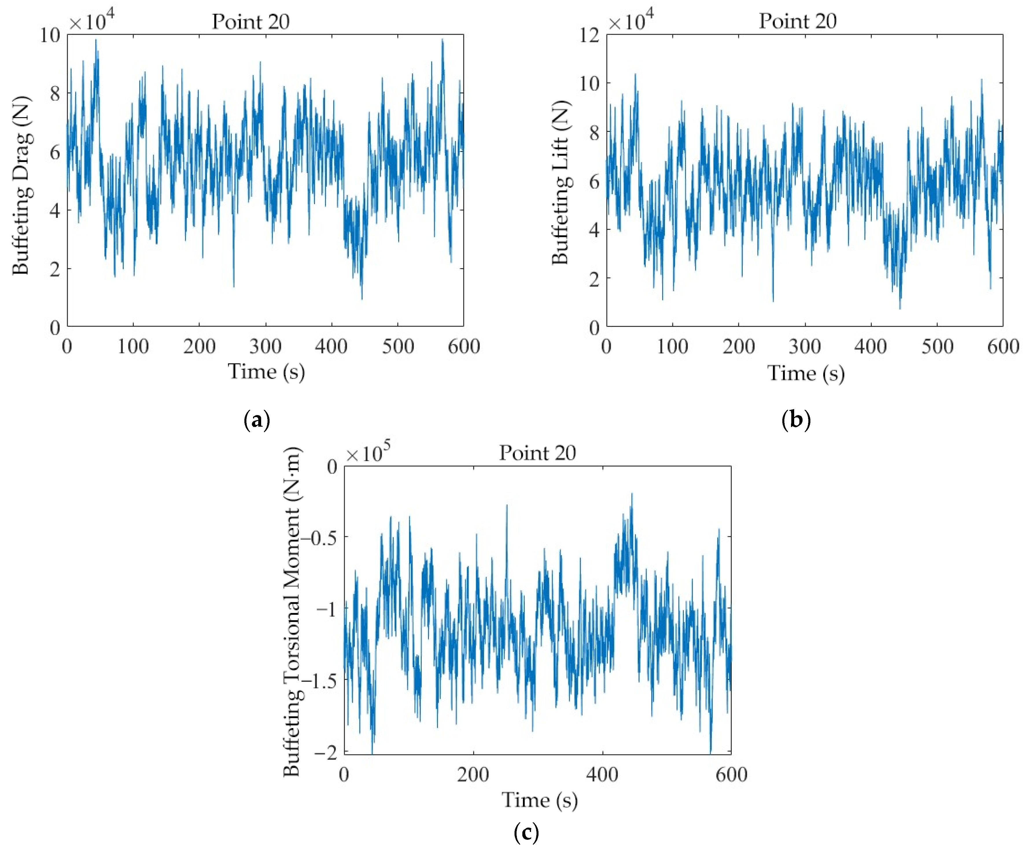
Using the wind tunnel-derived coefficient–angle-of-attack fits (Equations (55)–(60)) and their derivatives (Equations (61)–(66)), the instantaneous angle of attack α(t) from the fluctuating wind is substituted at each time step to obtain the force and moment coefficients. These are then converted, as needed, to the wind axis three-component form and substituted into the Davenport quasi-steady relations (Equations (27)–(29)), together with the synthesized wind speeds, to generate the segment-wise line load time histories of the drag, lift, and pitching moment, as shown in Figure 30.
Figure 30 shows all three traces fluctuating about zero with stable amplitudes. The drag and lift vary in step, while the pitching moment exhibits larger fluctuations, occasional higher peaks, and a slight negative bias. Relative to the 3F-based results, the drag and lift are comparable, but the pitching moment is more pronounced, indicating a more evident torsional response in the subsequent structural analysis.
(2)
Time-Domain Buffeting Analysis
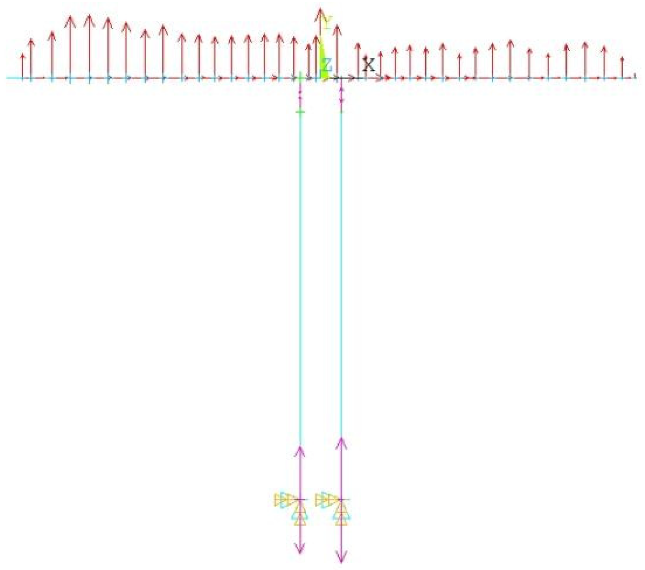
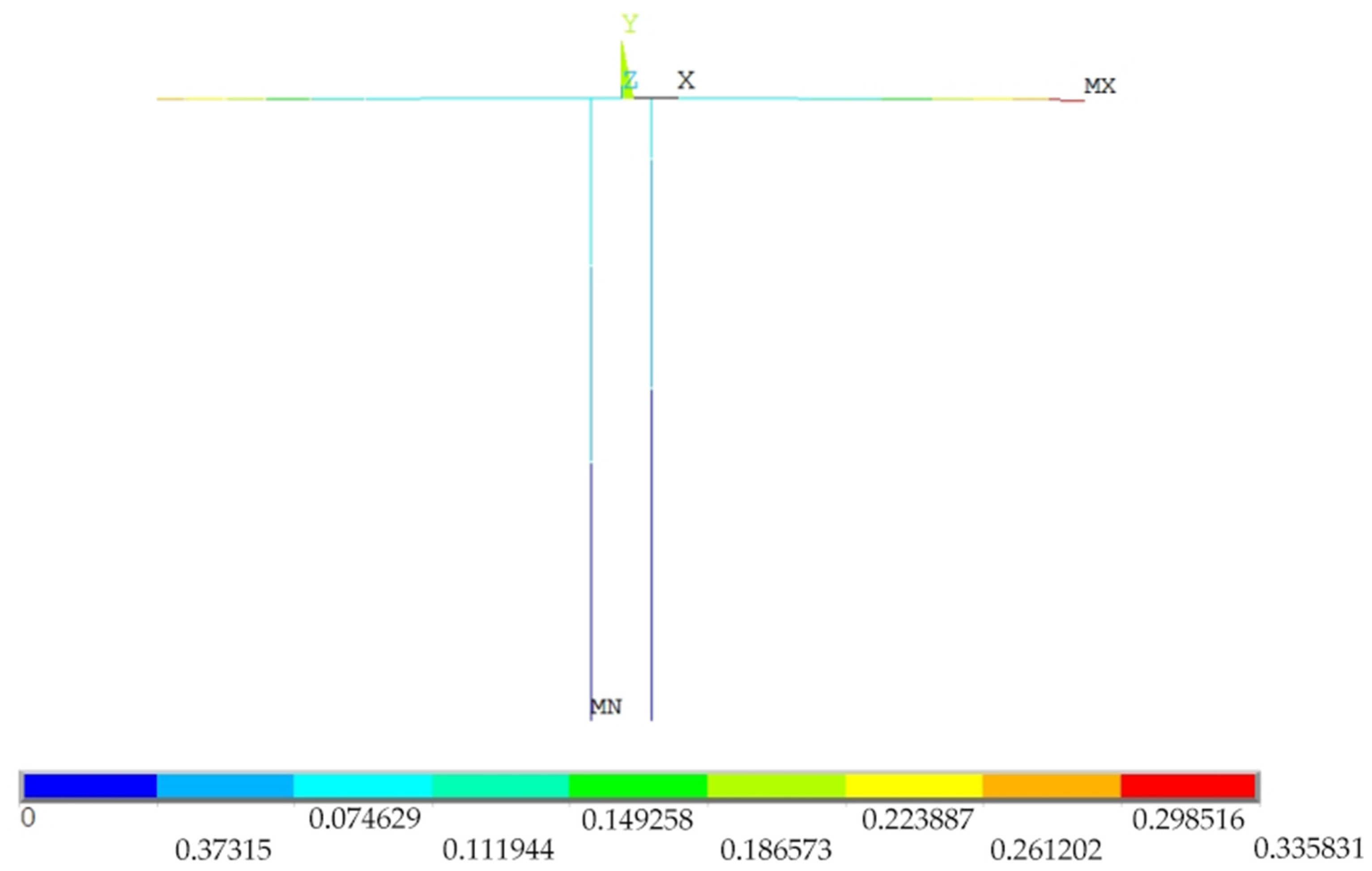
Using APDL secondary development, a time-domain buffeting analysis was performed. The nodal loading layout for the construction-stage girder is shown in Figure 31 and the global deformed shape is shown in Figure 32.
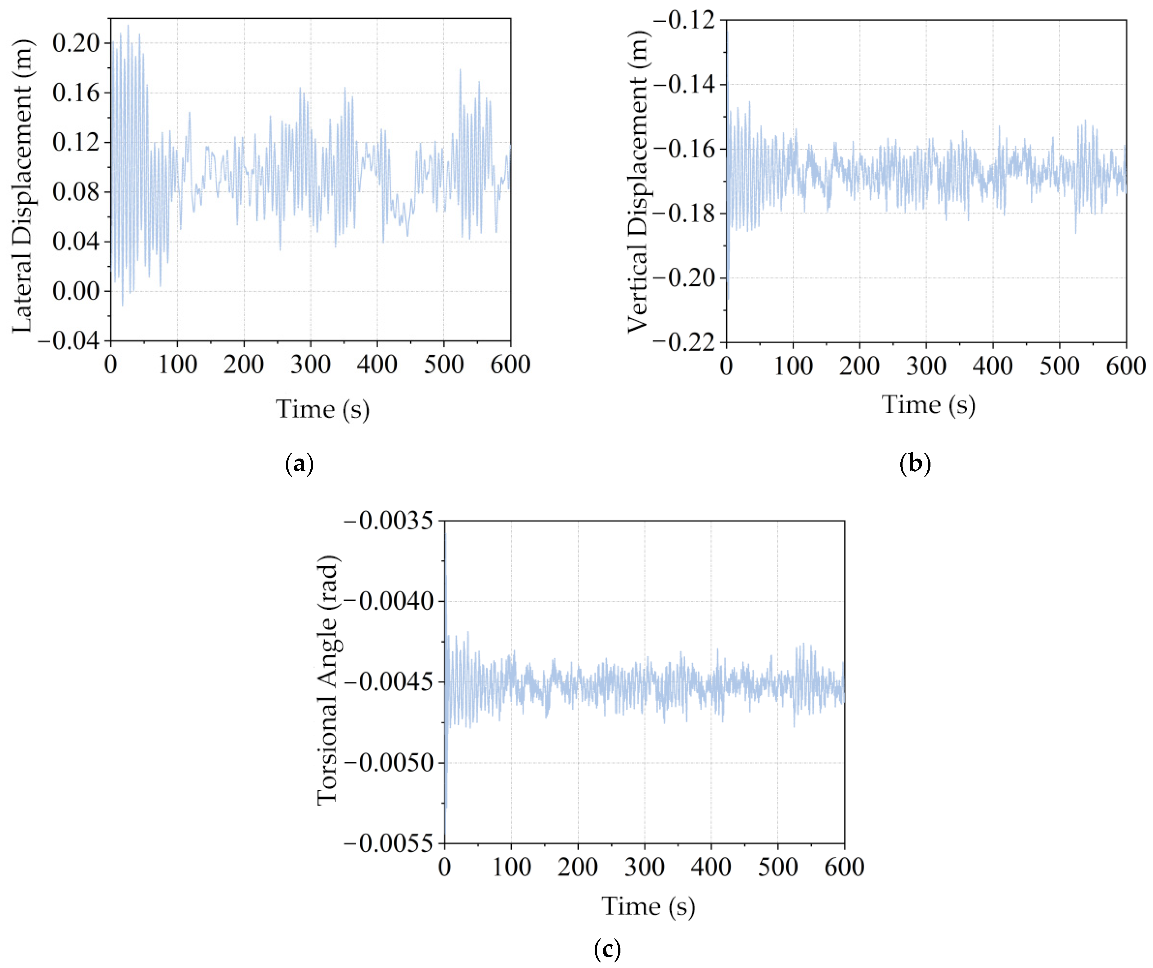
The deformation plot indicates that the right cantilever tip is the controlling location, while the midspan deformation is relatively small. Accordingly, that tip section is selected as the representative location: its lateral and vertical acceleration time histories (Figure 33) exhibit zero-mean, narrow-band random fluctuations; the displacement and torsional angle time histories (Figure 34) show lateral displacement fluctuating around approximately 0.12 m, vertical displacement around −0.18 m, and torsional rotation around −4.5 × 10⁻³ rad, with no drift trend, indicating linear elastic behavior at the present wind speed level.
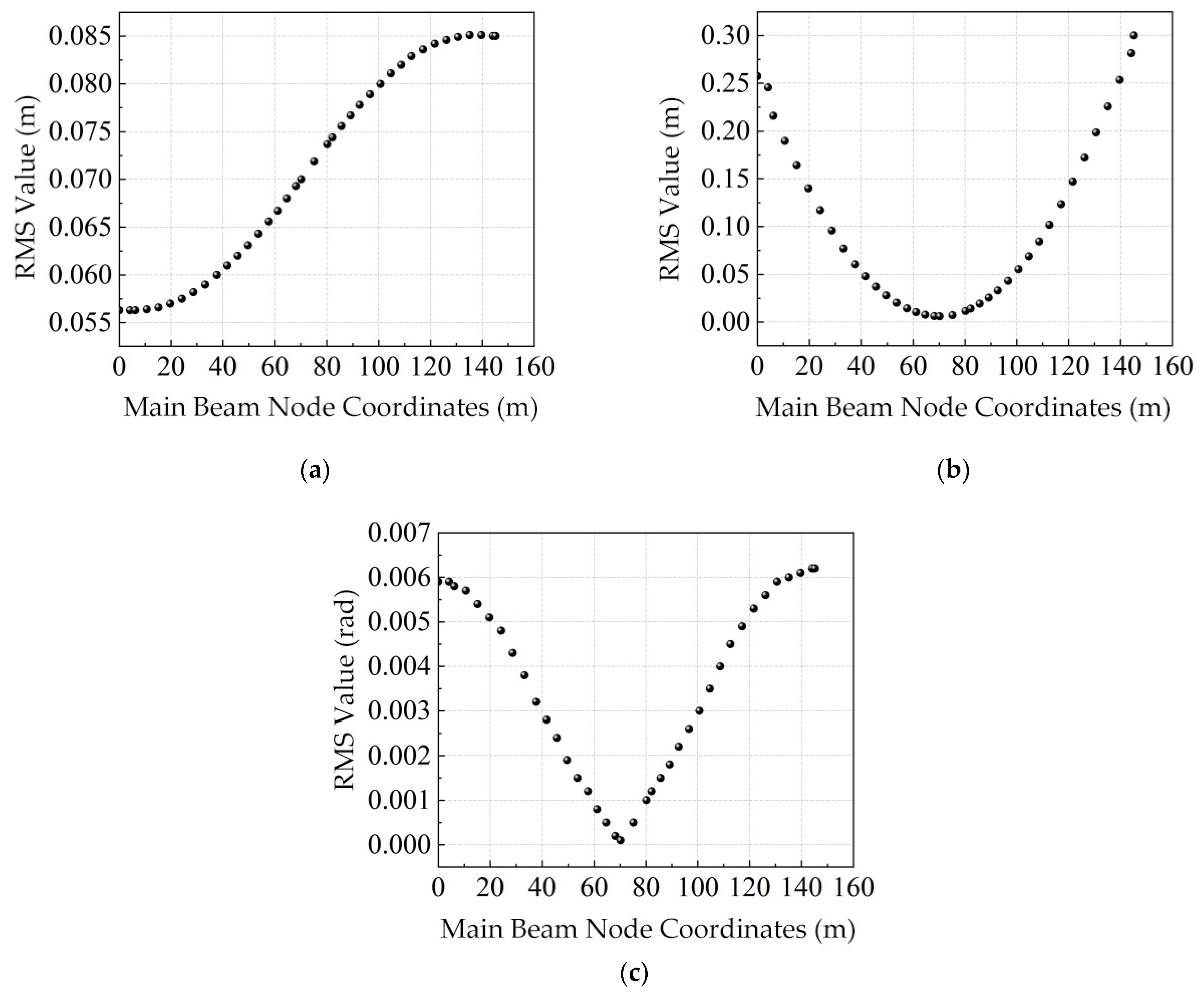
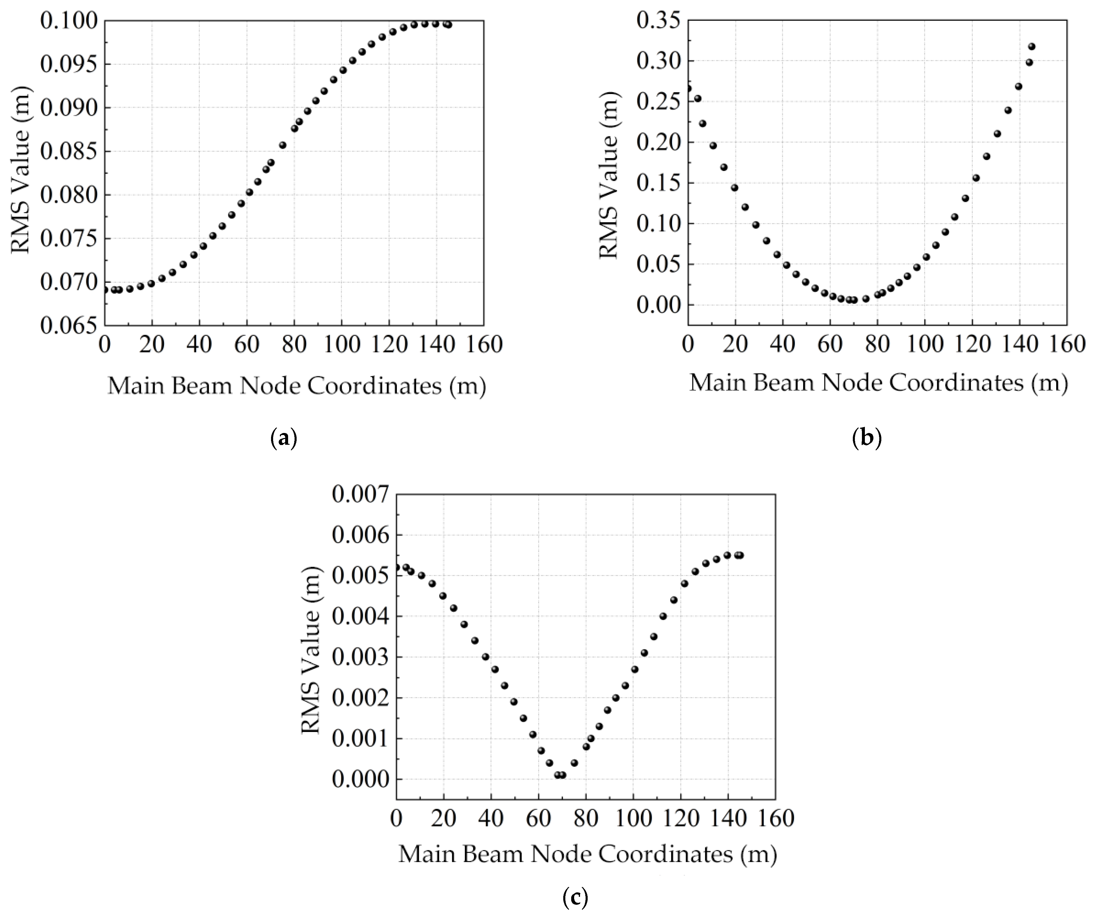
Based on the wind tunnel six-component inputs, the RMS values of the three DOF displacements at each girder node are plotted in Figure 35.
As shown in Figure 35, the along-span RMS distributions indicate that the lateral displacement increases monotonically from the pier toward the cantilever tip, while the vertical displacement and torsional rotation follow a “small near midspan, larger at both ends” pattern, which means that the free cantilever tip is more sensitive to the fluctuating wind.
A comparison between the aerostatic results and the buffeting peak responses (based on the wind tunnel inputs) during the construction stage is given in Table 11.
At the right cantilever tip, the amplification factors range from 2.159 to 2.767, with the torsional rotation showing the most pronounced increase. Overall, the amplification factors for the lateral, vertical, and torsional responses derived from the wind tunnel-based loading are of similar magnitude and relatively stable.

3.3. Numerical–Experimental Comparison

(1)
RMS distribution comparison
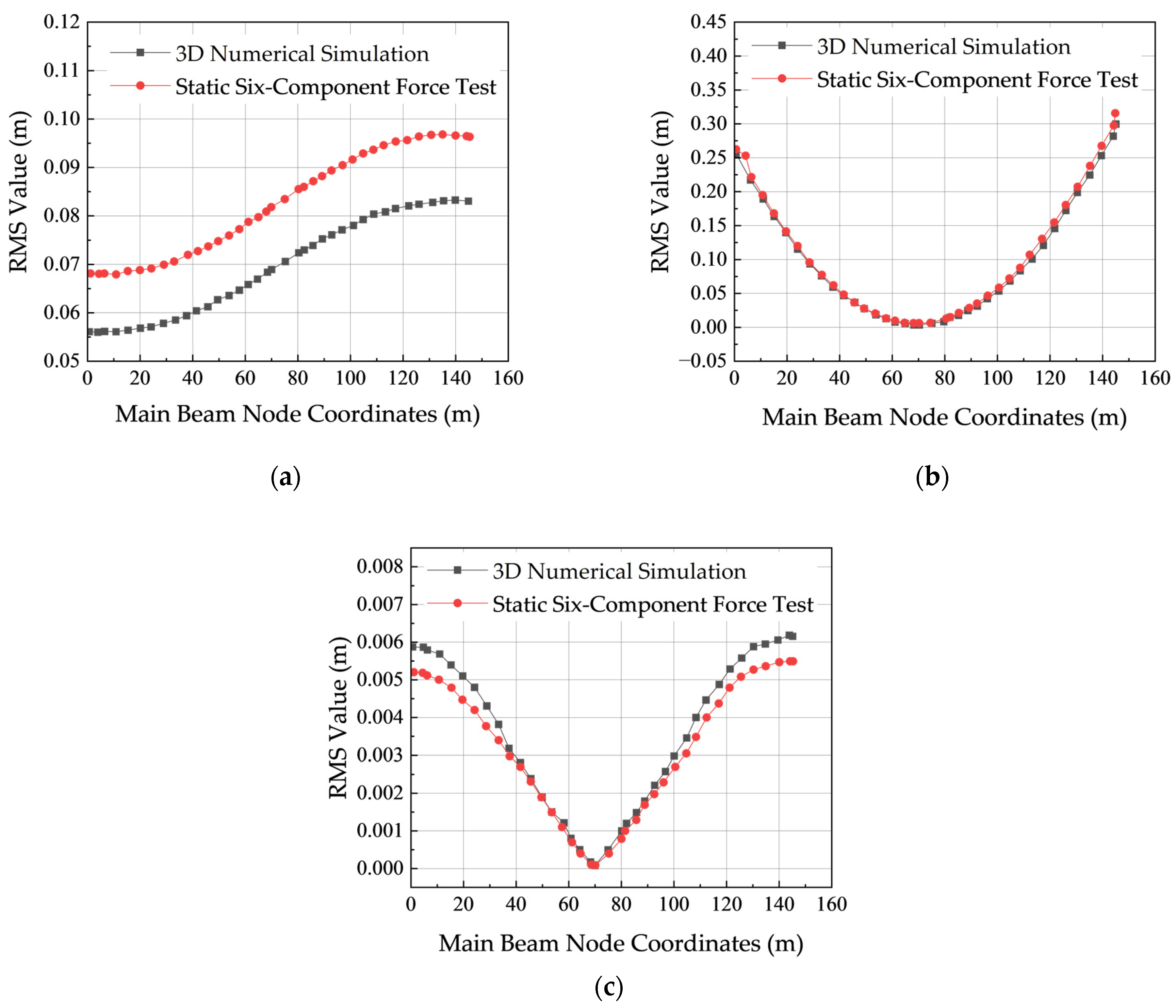
The RMS values of the three-DOF displacements at all girder nodes, obtained from the three-component-based time-domain analysis and from the six-component-based analysis, are compared in Figure 36.
From Figure 36, the two approaches exhibit the same overall patterns: the lateral displacement increases progressively from the pier toward the cantilever tip; the vertical displacement and torsional rotation show a clear “smaller at mid-span, larger near both ends” trend. In terms of magnitudes, the differences in vertical and torsional RMS are small—mean square error within 1%, nRMSE < 10%, and peak locations are essentially coincident. For the lateral RMS, the discrepancy is larger—mean square error 1.29% and nRMSE 44.55%—primarily near the cantilever tip. The detailed side-by-side comparison is summarized in Table 12.
In summary, the two approaches provide comparable predictions in the dominant modal frequency range.
(2)
Comparison of buffeting amplification factors
By comparing the buffeting peaks at representative nodes with the aerostatic baselines, the buffeting amplification factors are shown in Figure 37.
The buffeting amplification factor quantifies the increase in the total wind-induced response relative to the aerostatic response under the action of fluctuating wind, and is an important parameter for design and safety evaluation [34,35]. As seen in Figure 36, the numerically simulated amplification factors (lateral displacement, vertical displacement, and torsional rotation) exhibit a mean, standard deviation, and coefficient of variation of 2.58, 0.63, and 24.38%, respectively; the wind tunnel measurements yield corresponding values of 2.49, 0.31, and 12.37%. Thus, the amplification factors obtained using the six-component wind tunnel inputs are smaller and exhibit a narrower spread than those from the numerical three-component inputs, indicating improved accuracy and reduced uncertainty when the six-component coefficients are employed.

4. Conclusions

This study focuses on the maximum twin-cantilever construction stage of the Youlian Honghe Grand Bridge. Under the same target spectrum and the same full-bridge FE model, we establish and compare two routes—“3F 3D numerical time-domain analysis” and “6F 3D sectional wind tunnel time-domain analysis” to evaluate buffeting. The comparison centers on main girder RMS displacements and the buffeting amplification factor. The main conclusions are as follows:
(1) Fluctuating wind input. The multi-point wind speed time histories synthesized by harmonic superposition agree well with the target spectra, the spectral error within the dominant band is <10%, the standard deviation bias is <5%, and the mean square error of coherence for representative sensor pairs is <0.02, providing reliable input for buffeting analysis.
(2) Three-dimensional segment aerodynamics. Using a 3D segment “numerical wind tunnel” (steady RANS, standard k–ω), drag, lift, and pitching moment coefficients and their angle-of-attack derivatives were obtained. The overall trends are as follows: drag decreases with the increasing angle of attack; lift shows a near-parabolic variation with a peak at a small negative angle; and the pitching moment coefficient varies monotonically and is more sensitive to the angle of attack. The fitted functions can be directly used in time-domain load calculations.
(3) Aerostatic baseline and stability. An APDL FE model was built for the construction stage. The displacement–wind speed curves indicate a critical aerostatic wind speed of about 140 m/s. At the test wind speed 28 m/s and the design wind speed 34.52 m/s, the structure remains in a stable operating range, serving as the baseline for buffeting superposition.
(4) Spatial distribution and magnitude of buffeting response. At 28 m/s, RMS lateral and vertical displacements and torsional rotation along the girder are larger at the cantilever ends and smaller near midspan, with the right tip being most unfavorable. The amplification factors at the representative tip are approximately 1.9 (lateral), 2.7 (vertical), and 3.1 (torsion), indicating higher torsional sensitivity to fluctuating wind.
(5) Three-component time-domain vs. six-component comparison. Driven by six-component coefficients and their derivatives, the time-domain analysis shows overall agreement with the three-component framework in peak locations, along-span trends, and the dominant frequency band (0.19~0.26 Hz). The RMS errors at the main girder nodes are RMSE = 0.0129, 0.0064, 0.0004 (lateral, vertical, torsional), with range-normalized nRMSE = 0.4455, 0.0208, 0.0976, indicating the best consistency in the vertical channel, followed by torsional, while lateral differences concentrate near the cantilever tip. For the buffeting amplification factor, the statistics for numerical simulation (3F) versus wind tunnel testing (6F) are as follows: mean 2.58, 2.49; standard deviation 0.63, 0.31; and coefficient of variation 24.38%, 12.37%. Hence, the six-component route yields slightly smaller averages and notably lower dispersion, better capturing force–moment coupling and providing more robust predictions of torsional response, serving as a practical benchmark for cases with angle-of-attack sensitivity or pronounced sectional variation.
(1)
Applicability and limitations.
At the level of modeling assumptions: (i) the quasi-steady (QSA) framework treats instantaneous aerodynamic forces as adjusting immediately to inflow fluctuations, which may underestimate non-stationary phase lag at higher frequencies and increase sensitivity to the input spectrum; (ii) the absence of an explicit frequency-dependent aerodynamic admittance correction (effectively taking the admittance as 1) is a conservative treatment and may lead to slightly inflated responses at locations with weak spanwise coherence; and (iii) the numerical analysis employs an RANS (steady k–ω) model, which, while stable and controllable, is conservative in representing local separation and transient vortices, potentially flattening the slope of aerodynamic derivatives over certain angle-of-attack ranges and introducing some uncertainty in assessing force–moment coupling.
To manage the above effects and ensure engineering applicability, we confine our conclusions to the validated operating domain: angle of attack α ∈ [−10°, 10°] (step 2°), representative wind speed 28 m/s (with a comparative case at 34.52 m/s), dominant energy band 0.19~0.26 Hz, and total simulation duration 600 s. On the input side, we enforce target-spectrum consistency and multi-point coherence checks—spectral error in the dominant band < 10%, standard deviation bias < 5%, and mean square coherence error < 0.02—to mitigate the influence of the QSA assumption and the uncorrected admittance. In parallel, we implement a six-component and three-component comparison under the same FE model and wind input, attributing discrepancies as far as possible to the aerodynamic inputs themselves; the RMS peak and buffeting amplification factor at the cantilever-end representative point are used as verifiable engineering indicators to identify torsion-dominated and angle-of-attack-sensitive cases. If, within the validated domain, torsional dominance or a marked divergence between the six-component and three-component results is observed, we recommend prioritizing the six-component baseline for verification and explicitly stating the assumptions and applicability range to ensure the reliability of the conclusions.
(2)
Engineering notes.
For each verification: confirm input consistency (spectral error < 10%, stdev bias < 5%, coherence MSE < 0.02); evaluate on the same angle of attack grid (α = −10°:2°:10°), prioritizing 28 m/s (extend to 34.52 m/s if needed); keep the sectional test and FE model geometrically consistent (variable sections, end effects) and check within 0.19~0.26 Hz whether vertical and torsional responses dominate, especially at cantilever ends; finally, report RMS, peaks, and the buffeting amplification factor to inform safety margins and temporary measures.

Author Contributions

Conceptualization, L.D. and C.T.; methodology, L.D.; software, L.D.; validation, C.T. and J.J.; formal analysis, C.T.; investigation, J.J.; resources, J.J.; data curation, J.J.; writing—original draft preparation, L.D.; writing—review and editing, L.D.; visualization, L.D.; supervision, L.D. and C.T.; project administration, J.J.; funding acquisition, C.T. All authors have read and agreed to the published version of the manuscript.

Funding

This research received no external funding.

Data Availability Statement

Data supporting reported results are available from the author upon request.

Conflicts of Interest

The authors declare no conflicts of interest.

References

  1. Chen, Z. Wind-Induced Vibration Stability and Control of Engineering Structures; Science Press: Beijing, China, 2013. [Google Scholar]
  2. Wang, Q.; Zhang, W.; Chen, R. Review of research methods on wind-induced vibration of mountain bridges. Highway 2024, 69, 149–153. [Google Scholar]
  3. Diana, G.; Fiammenghi, G.; Belloli, M.; Rocchi, D. Wind tunnel tests and numerical approach for long span bridges: The Messina Bridge. J. Wind Eng. Ind. Aerodyn. 2013, 122, 38–49. [Google Scholar] [CrossRef]
  4. Wu, B.; Zhou, J.; Li, S.; Liu, Z.; Wu, Y. Combining active and passive wind tunnel tests to determine the aerodynamic admittances of a bridge girder. J. Wind Eng. Ind. Aerodyn. 2022, 231, 105180. [Google Scholar] [CrossRef]
  5. Diana, G.; Omarini, S. A non-linear method to compute the buffeting response of a bridge—Validation of the model through wind tunnel tests. J. Wind Eng. Ind. Aerodyn. 2020, 201, 104163. [Google Scholar] [CrossRef]
  6. Yi, S.; Jin, D.; Li, S.; Jian, B.; Liu, J. Buffeting response prediction of long-span bridges based on different wind tunnel test techniques. Appl. Sci. 2022, 12, 3171. [Google Scholar] [CrossRef]
  7. Taylor, I.; Vezza, M. A numerical investigation into the aerodynamic characteristics and aeroelastic stability of a footbridge. J. Fluids Struct. 2008, 25, 155–177. [Google Scholar] [CrossRef]
  8. Hallak, H.P.; Pfeil, S.M.; Oliveira, D.R.S.; Battista, R.C.; de Sampaio, P.A.; Bezerra, C.M. Aerodynamic behavior analysis of Rio–Niterói Bridge by means of computational fluid dynamics. Eng. Struct. 2013, 56, 935–944. [Google Scholar] [CrossRef]
  9. Liu, L. Application of CFD in Aerodynamic Control Measures for Long-Span Bridges. Master’s Thesis, Wuhan University of Technology, Wuhan, China, 2007. [Google Scholar]
  10. Gao, Y.; Wang, H.; Xu, Z.; Tao, T.; Wang, F.; Xie, Y. Numerical simulation of aerostatic three-component coefficients of box-girder sections for long-span high-speed railway continuous bridges. J. Nanjing Univ. Technol. (Nat. Sci. Ed.) 2020, 42, 358–365. [Google Scholar]
  11. Davenport, A.G.; Agnew, R.; Harris, R.I. The application of statistical concepts to the wind loading of structures. Proc. Inst. Civ. Eng. 1961, 19, 449–472. [Google Scholar] [CrossRef]
  12. Jain, A.; Jones, N.P.; Scanlan, R.H. Coupled flutter and buffeting analysis of long-span bridges. J. Struct. Eng. 1996, 122, 716–725. [Google Scholar] [CrossRef]
  13. Caracoglia, L. Influence of uncertainty in selected aerodynamic and structural parameters on the buffeting response of long-span bridges. J. Wind Eng. Ind. Aerodyn. 2007, 96, 327–344. [Google Scholar] [CrossRef]
  14. Zhao, L.; Ge, Y. Sensitivity of buffeting response considering multi-component aerodynamic admittance. J. Vib. Shock 2010, 29, 84–88. [Google Scholar]
  15. Yang, Y.; Liao, H.; Li, Y. A practical time-domain method for buffeting analysis of cable-stayed bridges based on ANSYS. Acta Aerodyn. Sin. 2004, 22, 457–460. [Google Scholar]
  16. Zeng, X.; Han, D. Time-domain analysis of wind-induced buffeting of long-span bridges and its implementation in ANSYS. Bridge Constr. 2004, 1, 9–12. [Google Scholar]
  17. Calamelli, F.; Rossi, R.; Argentini, T.; Rocchi, D.; Diana, G. A nonlinear approach for the simulation of the buffeting response of long-span bridges under non-synoptic storm winds. J. Wind Eng. Ind. Aerodyn. 2024, 247, 105681. [Google Scholar] [CrossRef]
  18. Fenerci, A.; Øiseth, O. Measured buffeting response of a long-span suspension bridge compared with numerical predictions based on design wind spectra. J. Struct. Eng. 2017, 143, 04017131. [Google Scholar] [CrossRef]
  19. JTG/T 3360-01-2018; Research Institute of Highway, Ministry of Transport (Tongji University). Wind-Resistant Design Code for Highway Bridges. People’s Transportation Press: Beijing, China, 2019.
  20. Xu, Y.L.; Sun, D.K.; Ko, J.M.; Lin, J.H. Buffeting analysis of long span bridges: A new algorithm. Comput. Struct. 1998, 68, 303–313. [Google Scholar] [CrossRef]
  21. Morgenthal, K. Modelling Techniques for Buffeting Analysis of Long-span Bridges. In Proceedings of the IABSE Conference—Bridges and Structures Sustainability—Seeking Intelligent Solutions, Guangzhou, China, 8–11 May 2016; pp. 221–228. [Google Scholar]
  22. Shen, Z.; Li, J.; Gao, G.; Xue, X.F. Buffeting response of a composite cable-stayed bridge in a trumpet-shaped mountain pass. Adv. Struct. Eng. 2019, 23, 510–522. [Google Scholar] [CrossRef]
  23. da Costa, B.M.; Wang, J.; Jakobsen, J.B.; Øiseth, O.A.; þór Snæbjörnsson, J. Bridge buffeting by skew winds: A revised theory. J. Wind Eng. Ind. Aerodyn. 2022, 220, 104806. [Google Scholar] [CrossRef]
  24. Zhu, L.; Zhou, Q.; Ding, Q.; Xu, Z. Identification and application of six-component aerodynamic admittance functions of a closed-box bridge deck. J. Wind Eng. Ind. Aerodyn. 2018, 172, 268–279. [Google Scholar] [CrossRef]
  25. Wu, Y.; Chen, Y.; Geng, W.; Xu, X.; Lai, Y. A frequency-dependent uniform discretization scheme for simulating fluctuating wind field based on a frequency–wavenumber spectrum. J. Wind Eng. Ind. Aerodyn. 2024, 244, 105628. [Google Scholar] [CrossRef]
  26. Bekele, S.; Hangan, H. A comparative investigation of the TTU pressure envelope: Numerical versus laboratory and full-scale results. Wind Struct. 2002, 5, 337–346. [Google Scholar] [CrossRef]
  27. Wu, F.; Zhang, Q. Study on three-component coefficients of a double-box composite-girder cable-stayed bridge. Eng. Constr. 2024, 38, 762–765. [Google Scholar]
  28. Gao, H.; Wang, F.; Guan, Q.; Hou, H.; Li, J. Research on the flutter stability of bridge sections based on an empirical formula of an aerostatic three-component coefficient. Buildings 2022, 12, 1212. [Google Scholar] [CrossRef]
  29. Wu, X. Numerical Study on Three-Component Coefficients of the Main Girder of High-Pier Long-Span Continuous Rigid-Frame Bridges. Master’s Thesis, Central South University, Changsha, China, 2010. [Google Scholar]
  30. Zhang, W.; Ge, Y. An iterative optimization method for nonlinear aerostatic stability of long-span bridges. In Proceedings of the 14th National Conference on Structural Wind Engineering, Nanjing, China, 27–30 August 2009. [Google Scholar]
  31. Guang, Z. Nonlinear Aerostatic Stability Analysis of Long-Span Suspension Bridges. Master’s Thesis, Chang’an University, Xi’an, China, 2022. [Google Scholar]
  32. Wang, L.; Shi, F.; Wang, Z.; Liang, S. Blockage effects in wind tunnel tests for tall buildings with surrounding buildings. Appl. Sci. 2022, 12, 7087. [Google Scholar] [CrossRef]
  33. Wei, G. Study on Six-Component Force Coefficients in Bridge Wind Tunnel Tests. Master’s Thesis, Chang’an University, Xi’an, China, 2009. [Google Scholar]
  34. GB 50009-2012; Ministry of Housing and Urban–Rural Development of the PRC. Load Code for the Design of Building Structures. China Architecture & Building Press: Beijing, China, 2012.
  35. Xie, W. Analysis of Wind-Induced Buffeting Response of High-Pier Long-Span Continuous Rigid-Frame Bridges in Mountainous Areas. Master’s Thesis, Wuhan University of Technology, Wuhan, China, 2019. [Google Scholar]
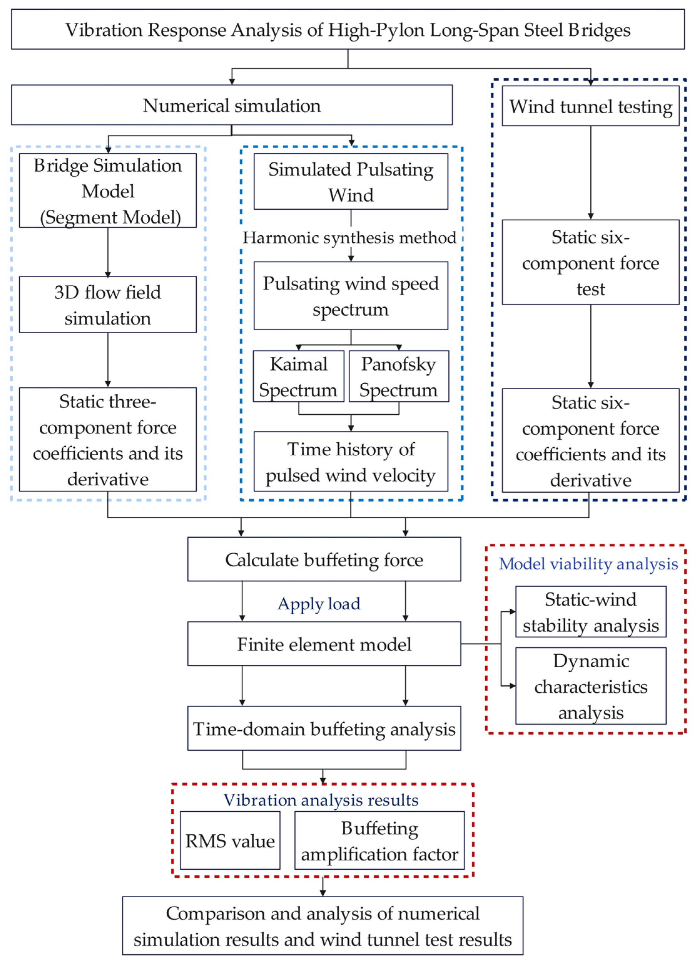
Figure 1. Technical workflow diagram.
Buildings 15 03715 g001
Figure 2. Layout of the main bridge of the Youlian Honghe Bridge.
Buildings 15 03715 g002
Figure 3. Elevation of Main Bridge 2.
Buildings 15 03715 g003
Figure 4. Schematic of the main girder cross-section.
Buildings 15 03715 g004
Figure 5. Three-dimensional simulation model of the Youlian Honghe Bridge.
Buildings 15 03715 g005
Figure 6. Layout of measurement points.
Buildings 15 03715 g006
Figure 7. Along-wind fluctuating wind time history: (a) along-wind fluctuating wind time history at Point 1; (b) along-wind fluctuating wind time history at Point 20.
Buildings 15 03715 g007
Figure 8. Vertical fluctuating wind time history: (a) vertical fluctuating wind time history at Point 1; (b) vertical fluctuating wind time history at Point 20.
Buildings 15 03715 g008
Figure 9. Target-spectrum fitting of the along-wind component: (a) target-spectrum fit for along-wind PSD at Point 1; (b) target-spectrum fit for along-wind PSD at Point 20.
Buildings 15 03715 g009
Figure 10. Target-spectrum fitting of the vertical component: (a) target-spectrum fit for vertical PSD at Point 1; (b) target-spectrum fit for vertical PSD at Point 20.
Buildings 15 03715 g010
Figure 11. Segment layout of the main girder.
Buildings 15 03715 g011
Figure 12. Local mesh refinement around the bridge.
Buildings 15 03715 g012
Figure 13. Simulation results of Segment 1 at α = 0°: (a) pressure contours of Segment 1 at α = 0°; (b) streamlines of Segment 1 at α = 0°.
Buildings 15 03715 g013
Figure 14. Simulation results of Segment 1 at α = 10°: (a) pressure contours of Segment 1 at α = 10°; (b) streamlines of Segment 1 at α = 10°.
Buildings 15 03715 g014
Figure 15. Finite-element model of the T-type structure at the maximum double-cantilever construction stage.
Buildings 15 03715 g015
Figure 16. Displacement–wind speed curves: (a) lateral displacement–wind speed curve; (b) vertical displacement–wind speed curve; (c) torsional angle–wind speed curve.
Buildings 15 03715 g016
Figure 17. First ten mode shapes during the construction stage: (a) Mode 1; (b) Mode 2; (c) Mode 3; (d) Mode 4; (e) Mode 5; (f) Mode 6; (g) Mode 7; (h) Mode 8; (i) Mode 9; (j) Mode 10.
Buildings 15 03715 g017aBuildings 15 03715 g017b
Figure 18. Photographs of the static six-component wind tunnel test: (a) side view of the model; (b) front view of the model.
Buildings 15 03715 g018
Figure 19. Variation in three-component coefficients with angle of attack (Segment 1).
Buildings 15 03715 g019
Figure 20. Variation in three-component coefficients with angle of attack (Segment 3).
Buildings 15 03715 g020
Figure 21. Static triaxial coefficient fitting curve.
Buildings 15 03715 g021
Figure 22. Buffeting force time histories at the midspan node: (a) time history of buffeting drag; (b) time history of buffeting lift; (c) time history of buffeting torque moment.
Buildings 15 03715 g022
Figure 23. Nodal loading layout on the main girder.
Buildings 15 03715 g023
Figure 24. Global deformed shape (structural displacement).
Buildings 15 03715 g024
Figure 25. Acceleration time histories at the tip of the maximum double-cantilever configuration: (a) lateral acceleration time history; (b) vertical acceleration time history.
Buildings 15 03715 g025
Figure 26. Displacement and rotation time histories at the tip of the maximum double-cantilever configuration: (a) lateral displacement time history; (b) vertical displacement time history; (c) torsional angle time history.
Buildings 15 03715 g026
Figure 27. RMS displacement of the main girder: (a) RMS of lateral displacement of the main girder; (b) RMS of vertical displacement of the main girder; (c) RMS of torsional rotation of the main girder.
Buildings 15 03715 g027
Figure 28. Static six-component force coefficients for full-bridge model.
Buildings 15 03715 g028
Figure 29. Six-degree-of-freedom coefficient fitting curve.
Buildings 15 03715 g029
Figure 30. Buffeting force time histories at the midspan node: (a) time history of buffeting drag; (b) time history of buffeting lift; (c) time history of buffeting torsional moment.
Buildings 15 03715 g030
Figure 31. Nodal loading layout on the main girder.
Buildings 15 03715 g031
Figure 32. Global deformed shape.
Buildings 15 03715 g032
Figure 33. Acceleration time histories at the tip of the maximum double-cantilever configuration: (a) lateral acceleration time history; (b) vertical acceleration time history.
Buildings 15 03715 g033
Figure 34. Displacement and rotation time histories at the tip of the maximum double-cantilever configuration: (a) lateral displacement time history; (b) vertical displacement time history; (c) torsional angle time history.
Buildings 15 03715 g034
Figure 35. RMS displacement of the main girder: (a) RMS of lateral displacement of the main girder; (b) RMS of vertical displacement of the main girder; (c) RMS of torsional rotation of the main girder.
Buildings 15 03715 g035
Figure 36. Comparison of nodal RMS displacements of the main girder: (a) comparison of RMS lateral displacement of the main girder; (b) comparison of RMS vertical displacement of the main girder; (c) comparison of RMS torsional rotation of the main girder.
Buildings 15 03715 g036
Figure 37. Comparison of buffeting amplification factors.
Buildings 15 03715 g037
Table 1. Parameters for fluctuating wind simulation.
ParameterValue
Ground roughness z00.16
Number of frequency samples N6000
Cutoff frequency ω (Hz)
Simulation duration t (s)600
Time step (s)t/N
Sampling interval Δt (s)0.25
Frequency increment (Hz)ω/N
Main bridge span (m)145.16
Design wind speed (m/s)28
Table 2. Numerical simulation parameters.
Computational ParametersValue
Turbulence intensity5%
Turbulence viscosity ratio10
Air density (kg/m3)1.225
Air dynamic viscosity [kg/(m·s)]1.7894 × 10−5
Inflow wind speed (m/s)28
Table 3. Material properties for the finite-element model.
LocationMaterialElastic Modulus (MPa)Poisson’s RatioDensity (kg/m3)
Main girderC55 reinforced concrete3.55 × 1040.22500
Main pierC50 reinforced concrete3.45 × 1040.22500
Table 4. Equivalent static gust wind speeds by construction block (construction stage).
BlockSegment-Center Height Above Ground (m)Reference Wind Speed (m/s)Equivalent Static Gust Wind Speed (m/s)
1#Block 91.58339.10650.838
2#Block 91.60439.10750.840
3#Block 91.56439.10550.836
4#Block 91.55639.10450.835
5#Block 91.51939.10250.832
6#Block 91.45539.09750.826
7#Block 91.36639.09150.818
8#Block 91.25439.08350.808
9#Block 91.12039.07450.797
10#Block 90.97539.06450.784
11#Block 90.81139.05350.769
12#Block 90.63139.04150.753
13#Block 90.43539.02750.735
14#Block 90.22339.01250.716
15#Block 90.01238.99850.697
16#Block 89.79238.98350.677
17#Block 89.56038.96650.656
18#Block 89.37238.95350.639
19#Block 89.27138.94650.630
20#Block 89.31238.94950.634
21#Block 89.58338.96850.658
22#Block 89.90338.9950.687
23#Block 90.30239.01850.723
24#Block 90.69039.04550.758
25#Block 91.08139.07250.793
26#Block 91.48539.09950.829
27#Block 91.87439.12650.864
28#Block 92.24639.15150.896
29#Block 92.60239.17550.928
30#Block 92.95039.19950.958
31#Block 93.30139.22250.989
32#Block 93.62939.24451.018
33#Block 93.93339.26551.044
34#Block 94.21339.28451.069
35#Block 94.46739.30051.091
36#Block 94.69039.31551.110
37#Block 94.88739.32851.127
Piers42.50034.58644.961
Table 5. Natural frequencies during the construction stage.
ModeFrequency (Hz)Mode Description
10.18882Pier bending (longitudinal)
20.21200Pier torsion
30.26118Pier bending (lateral)
40.76390Girder vertical bending, antisymmetric
51.15250Girder vertical bending, symmetric
61.24830Girder vertical bending, symmetric; pier bending (longitudinal), symmetric
71.36810Girder vertical bending, antisymmetric; pier bending (longitudinal)
81.60110Girder lateral bending, symmetric; pier bending (lateral)
92.37140Girder and pier lateral bending, second order, symmetric
102.72060Girder lateral bending, second order, symmetric; pier lateral bending, second order, antisymmetric
Table 6. Static three-component coefficients by girder segment.
SegmentAngle of Attack
(Deg)
Drag Coefficient
CD
Lift Coefficient
CL
Torque Coefficient CM
1−20.97451.9512−0.6351
00.94122.2459−0.4013
20.93972.1027−0.3126
2−20.80452.4146−0.3464
00.82732.2185−0.3006
20.79421.8846−0.2840
3−21.41361.2461−0.1946
01.45541.0189−0.1742
21.43990.9449−0.1678
4−21.38741.3154−0.1615
01.50011.1717−0.1426
21.47541.0346−0.1310
5−20.71562.4501−0.3045
00.76632.3302−0.2821
20.64552.1031−0.2644
6−20.98412.3594−0.4133
00.77782.3295−0.3913
20.69511.9422−0.3712
Table 7. Derivatives of three-component coefficients by girder segment.
SegmentAngle of Attack
(Deg)
Derivative of Drag Coefficient
CD
Derivative of Lift Coefficient
CL
Derivative of Torque Coefficient CM
1−20.03461 −0.06234 −0.01573
00.02472 −0.06460 −0.01612
20.01483 −0.06686 −0.01651
2−20.01349 −0.03745 −0.01387
00.00696 −0.02748 −0.01068
20.00043 −0.01751 −0.00749
3−2−0.01849 0.01672 −0.00671
0−0.01864 0.01432 −0.00520
2−0.01879 0.01192 −0.00369
4−2−0.01609 0.01896 −0.00259
0−0.01620 0.01792 −0.00312
2−0.01631 0.01688 −0.00364
5−20.02140 −0.04836 −0.00683
00.01284 −0.04136 −0.00468
20.00428 −0.03436 −0.00253
6−20.03668 −0.06962 −0.00351
00.03432 −0.06256 −0.00180
20.03196 −0.05550 −0.00010
Table 8. Wind-induced response during the construction stage.
Response TypeAerostatic ResponseBuffeting PeakTotal Wind-Induced ResponseBuffeting Amplification Factor
Lateral displacement (m)0.18510.16280.34791.88
Vertical displacement (m)−0.1343−0.23450.36882.746
Torsional rotation (rad)−0.0030−0.0063−0.00933.1
Table 9. Static six-component coefficients of the full-bridge model.
Angle of Attack (Deg)Drag Coefficient CDLift Coefficient CLSide Force Coefficient CORolling Moment Coefficient CMDYawing Moment Coefficient CMLPitching Moment Coefficient CMO
−100.85041.2783−0.33320.7946−0.4626−0.0981
−80.96490.7975−0.26660.7115−0.3351−0.1081
−61.02050.4650−0.23290.6449−0.1946−0.1199
−41.01680.2467−0.20090.5541−0.0419−0.1311
−21.03710.0557−0.19290.4478 0.1050 −0.1424
01.0221−0.1149−0.17780.32110.2164−0.1612
21.0010−0.2692−0.16410.41970.3249−0.1883
40.9776−0.3955−0.15200.51410.3915−0.2299
60.9479−0.5081−0.14190.62150.3256−0.2903
80.9098−0.6309−0.13170.73010.2494−0.3803
100.8721−0.7402−0.12350.8554 0.1440 −0.5012
Table 10. Static six-component coefficients of the full-bridge model (104).
Angle of Attack (Deg)Drag Coefficient CDLift Coefficient CLSide Force Coefficient CORolling Moment Coefficient CMDYawing Moment Coefficient CMLPitching Moment Coefficient CMO
−10−89.6682240.2358−38.673434.017863.776627.5030
−8−78.0545207.4286−32.986644.334335.221316.4424
−6−66.4409174.6215−27.299954.65076.66605.3818
−4−54.8273141.8143−21.613164.9671−21.8894−5.6788
−2−43.2136109.0072−15.926375.2836−50.4447−16.7394
0−31.600076.2000−10.239585.6000−79.0000−27.8000
2−19.986443.3928−4.552795.9164−107.5553−38.8606
4−8.372710.58571.1340106.2329−136.1106−49.9212
63.2409−22.22156.8208116.5493−164.6660−60.9818
814.8545−55.028612.5076126.8657−193.2213−72.0424
1026.4682−87.835818.1944137.1822−221.7766−83.1030
Table 11. Wind-induced response during the construction stage.
Response TypeAerostatic ResponseBuffeting PeakTotal Wind-Induced ResponseBuffeting Amplification Factor
Lateral displacement (m)0.18510.21460.39972.159
Vertical displacement (m)−0.1343−0.2066−0.34092.538
Torsional rotation (rad)−0.0030−0.0053−0.00832.767
Table 12. Comparison of RMS displacement differences at main girder nodes.
Response TypeLateral DisplacementVertical DisplacementTorsional Angle
RMSE0.0129 0.0064 0.0004
nRMSE (range-normalized)0.4455 0.0208 0.0976
Disclaimer/Publisher’s Note: The statements, opinions and data contained in all publications are solely those of the individual author(s) and contributor(s) and not of MDPI and/or the editor(s). MDPI and/or the editor(s) disclaim responsibility for any injury to people or property resulting from any ideas, methods, instructions or products referred to in the content.