Abstract
The digital recognition and preservation of historical architectural heritage has become a critical challenge in cultural inheritance and sustainable urban development. While deep learning methods show promise in architectural classification, existing models often struggle to achieve ideal results due to the complexity and uniqueness of historical buildings, particularly the limited data availability in remote areas. Focusing on the study of Chinese historical architecture, this research proposes an innovative architectural recognition framework that integrates the Swin Transformer backbone with a custom-designed Global Channel and Spatial Attention (GCSA) mechanism, thereby substantially enhancing the model’s capability to extract architectural details and comprehend global contextual information. Through extensive experiments on a constructed historical building dataset, our model achieves an outstanding performance of over 97.8% in key metrics including accuracy, precision, recall, and F1 score (harmonic mean of the precision and recall), surpassing traditional CNN (convolutional neural network) architectures and contemporary deep learning models. To gain deeper insights into the model’s decision-making process, we employed comprehensive interpretability methods including t-SNE (t-distributed Stochastic Neighbor Embedding), Grad-CAM (gradient-weighted class activation mapping), and multi-layer feature map analysis, revealing the model’s systematic feature extraction process from structural elements to material textures. This study offers substantial technical support for the digital modeling and recognition of architectural heritage in historical buildings, establishing a foundation for heritage damage assessment. It contributes to the formulation of precise restoration strategies and provides a scientific basis for governments and cultural heritage institutions to develop region-specific policies for conservation efforts.
1. Introduction
1.1. The Demand for Digital Information in Urban and Architectural Planning
In recent years, significant progress has been made nationwide in acquiring and applying digital information on urban environments and buildings, such as building category and material information, building health monitoring, street view, and satellite imagery. These data play an important role in architectural design and maintenance, urban planning, and policymaking. In China, many scholars have utilized deep learning models to extract features from urban street-view data to study urban architectural environments. For example, some studies have analyzed building environments through street-view data [1], explored their relationship with urban planning and design [2], and examined the visual perception of buildings and environments [3]. Additionally, some scholars have focused on the relationship between digital twin technologies and architectural heritage preservation, exploring the application of digital methods in heritage conservation [4].
Similar research has been conducted in other countries. For example, in Japan, scholars have analyzed residents’ perceptions of urban environments in Tokyo using street-view data [5]. In South Korea, scholars have combined digital information about urban architectural environments with the characteristics of surrounding commercial properties to analyze the urban architectural features of Seoul [6]. In India, scholars have employed various deep learning models to analyze architectural images, accurately identifying building types in multiple cities and mapping their spatial distributions [7]. In Europe, scholars have proposed a model updating method based on a particle swarm optimization algorithm to support restoration project designs and the implementation of structural health monitoring systems [8]. At the same time, some researchers have used historical time-series SVIs (Street View Images) and cyclist data from London to identify the causal impacts of specific architectural features on the number of urban cyclists [9]. In addition, another study has compared the effectiveness of different methods for detecting facade window layouts in New York and Lisbon [10]. In the United States, researchers have leveraged GIS, satellite imagery, and street-view data to obtain urban and architectural features to predict public perceptions of the built environment [11]. Some studies have used deep learning to analyze environmental information and investigate bus shelter distribution patterns across 20 cities in the United States [12]. Furthermore, researchers have utilized digital information on urban architecture from different countries and regions to compare buildings and environments across cities. For example, one study collected digital information on the architecture and urban environments from Amsterdam and Stockholm to compile a building age dataset, exploring the evolution of architectural styles and the spatial and temporal relationships between building age and style [13]. Another study analyzed over 250,000 architectural images from Singapore, San Francisco, and Amsterdam to examine the relationship between architecture and human perception [14]. Additionally, researchers have proposed a scalable framework to evaluate the Green View Index (GVI) using Mapillary images and image segmentation methods, assessing data completeness and utility in various geographical contexts across 11 cities, including Amsterdam, Barcelona, Melbourne, Seattle, and others [15].
However, compared to the richness of data available for modern cities, digital information on traditional dwellings and rural areas is relatively scarce. Globally, some traditional buildings are located in suburban or even remote mountainous regions, making data acquisition challenging [16,17,18]. With the acceleration of modernization, many traditional dwellings and villages around the world are at risk of disappearing [19,20,21,22]. For example, Gorica Ljubenov et al. explored the phenomenon of disappearing traditional buildings in the village of Stara Planina, located in the Pirot region on Serbia’s eastern border [23]. Additionally, HU, Die, and colleagues examined the effectiveness of China’s “Traditional Village” policy in the context of rapid urbanization. Using traditional villages in Jiangxi Province as a case study, their spatial analysis concluded the following: (1) the disappearance of traditional villages is most significant in areas near cities; and (2) the “Traditional Village” policy has, to some extent, prevented the loss of ancient village buildings and their historical heritage [24].
Therefore, building digital information systems for traditional dwellings and leveraging modern information technology for their preservation are of vital importance to ensure the sustainable development of these cultural heritage sites.
1.2. Application of Deep Learning Models
In the past, the data collection and classification of traditional urban and rural buildings and districts primarily relied on manual operations, which faced the challenges of low efficiency, poor accuracy, and high costs [25,26]. With the rapid advancement of artificial intelligence technology, researchers are now able to gather data in the architectural and urban fields at lower costs and at a higher speed. The application of deep learning models in this area has become increasingly widespread [27,28]. For example, Qing Han and colleagues constructed a labeled dataset and introduced transfer learning and automated data augmentation to use CNNs to classify traditional Chinese architectural styles [29]. Additionally, Daniela Gonzalez and colleagues used CNNs to automatically identify building materials and lateral force-resisting system types, thereby developing an exposure model for earthquake risk assessment [30]. Robin Roussel et al. proposed a deep convolutional neural network-based method that would improve building identification accuracy through multi-angle street view images and global optimization [31]. Menglin Dai and colleagues proposed a deep learning-based facade segmentation model for residential buildings using street-view images to precisely identify the components of the building facades and validated the model on real-world data from Sheffield, UK [32].
CNNs in deep learning have shown outstanding performance in tasks such as image detection and classification, semantic segmentation, and instance segmentation [33,34]. Moreover, with the successful application of Transformer architectures in natural language processing (NLP) applications such as ChatGPT, their use in computer vision has increasingly garnered attention from scholars. In recent years, a growing number of researchers have sought to apply Transformer models to image and video processing, achieving remarkable results. For instance, Changcheng Xiang et al. proposed a fast and robust safety helmet detection network based on a multiscale Swin Transformer, achieving real-time helmet detection in complex construction site scenarios and demonstrating excellent performance on public datasets [35]. Similarly, Girard Ludovic applied a Swin Transformer for rare subpixel target detection in hyperspectral imagery, achieving excellent classification results across multiple public datasets while significantly reducing memory usage [36]. In summary, deep learning technology offers researchers an efficient and cost-effective approach to acquiring and identifying information related to historical architectural heritage. Furthermore, the application of Transformer models in computer vision has shown strong developmental momentum, highlighting their vast potential in architectural and urban studies.
1.3. Challenges of Applying Deep Learning Models to Historical Buildings
The application of deep learning technology in the field of historical architectural heritage still faces many unresolved challenges. First, training deep learning models typically requires large volumes of high-quality images with rich detail, as well as precise annotations to ensure the reliability of the supervised information [37,38]. However, due to the remote location or protected status of certain historical buildings, acquiring comprehensive data on these structures is often difficult. Under such data limitations, model training processes are prone to issues of underfitting or overfitting [39,40,41], thereby affecting model performance. In terms of model selection, CNNs have demonstrated strong performance in computer vision tasks, especially in building image recognition and structural detection, making them widely applicable in architectural fields. However, CNNs have inherent limitations in feature extraction, as their local receptive field restricts the capture of long-range dependencies. Moreover, the hierarchical structure of CNNs extracts features sequentially from low to high level, leading to limitations in integrating global features [42,43,44]. As Transformers have recently excelled in natural language processing and computer vision, researchers have explored their application in building image recognition to address the local receptive field limitations of CNNs. Nevertheless, the use of Transformers in visual tasks also has limitations, such as a high computational complexity, strong dependence on large datasets, and insufficient capability to capture critical details. In building image recognition tasks, buildings often contain complex structural details and similar features, causing standard Transformers to perform suboptimally when processing high-resolution, large-scale images. Furthermore, they lack a direct modeling capacity for local features, potentially leading to an insufficient focus on key details [45,46,47].
In addition, although deep learning models have demonstrated strong performance across a wide range of computer vision tasks, their application in the specific field of historical building recognition still faces some challenges. Most mainstream models are trained on large-scale, widely distributed datasets of natural images or artificial objects, which typically contain rich and diverse images, thereby enabling favorable generalization capabilities in these domains. However, when these models are directly applied to specialized historical building datasets, questions remain as to whether their performance and generalizability can meet expectations [48,49,50].
Another key challenge for deep learning models in the field of historical building recognition lies in their limited interpretability. Although deep learning models, particularly those based on CNN and Transformer architectures, exhibit strong capabilities in feature extraction and pattern recognition, their internal feature extraction processes often remain “black-box” operations. When processing architectural images, these models rely on numerous parameters and complex network structures to automatically learn feature representations. However, this process lacks transparency, making it difficult for researchers to deeply understand the rationale behind the model’s historical building recognition and its decision-making logic [51,52].
1.4. Research Outcomes
Based on the challenges of applying deep learning technology to the preservation of historical architecture, this study conducted a series of targeted investigations and achieved the following outcomes:
- Through Internet data collection and field research, a substantial amount of primary data on historical buildings was obtained. Each data point was meticulously labeled, resulting in a high-quality, custom-built dataset. This dataset includes images of historical buildings from various regions, styles, and eras in China with detailed information to meet the training requirements of deep learning models.
- Building upon the Swin Transformer, a new deep learning model was developed by integrating the GCSA mechanism to enhance the performance of architectural image recognition. During the model training process, various regularization and data augmentation techniques were applied to effectively prevent overfitting, thereby ensuring the model’s robustness and generalizability.
- On the custom historical building dataset, the developed model achieved high accuracy in classification tasks, demonstrating its practicality and effectiveness in real-world applications. The Swin Transformer–GCSA model excels in historical building image classification and detail recognition tasks, showcasing strong capabilities in detail identification and image feature extraction.
- To improve the interpretability of the deep learning model, methods such as feature map analysis and Grad-CAM were employed to gain deeper insights into the model’s feature extraction process. These techniques reveal the model’s focus on different feature regions during architectural recognition, thereby making its decision-making logic more transparent.
In summary, this study provides an efficient tool for acquiring information on historical architectural heritage by constructing a high-quality dataset of historical buildings, developing an applicable deep learning model, and incorporating interpretability methods into the model. This approach effectively addresses the time-consuming and labor-intensive challenges of traditional manual classification and recognition methods, offering significant technical support for the sustainable development of historical buildings. Furthermore, the research findings contribute to the formulation of precise heritage restoration strategies and provide a scientific basis for governments and cultural heritage institutions to develop region-specific conservation policies.
2. Methods
2.1. Overall Workflow
The overall workflow and main procedures are illustrated in Figure 1, which includes their four major steps: data acquisition and processing, training and testing of various models, training and testing with different parameters, and interpretability analysis.
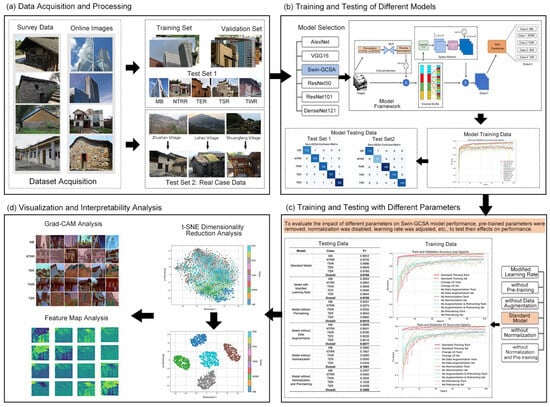
Figure 1.
Research framework.
First, to obtain a high-quality dataset, we combined field surveys with online resources to collect firsthand data. The dataset was divided into a training set, a validation set, and Test Set 1. Additionally, to better evaluate the model’s generalizability, the research team conducted fieldwork in traditional villages to gather architectural information on traditional dwellings, forming Test Set 2 to ensure the model’s reliability in real-world applications. For data preprocessing, data augmentation and data expansion techniques were applied to the Swin Transformer–GCSA model and other CNN models, along with transfer learning, standardization, and normalization to enhance model performance. During training, the convergence behavior and overfitting risk of each model were monitored on both the training and validation sets. Each model’s performance was subsequently evaluated on Test Set 1 and Test Set 2 to identify the optimal model. After selecting the optimal model, further analyses were conducted to assess its performance under various conditions, including the absence of data augmentation, transfer learning, or standardization, and using different learning rates. This step aims to reveal the impacts of data preprocessing, parameter adjustments, and pretraining on the model’s performance. Finally, to analyze the model’s decision-making mechanism, feature map visualization, t-SNE dimensionality reduction visualization, and Grad-CAM techniques were used. These methods helped unveil the features extracted by the model at different levels, analyzing its recognition and processing of input data, accurately locating the areas the model focuses on in specific prediction tasks, and providing an in-depth understanding of the model’s decision rationale and logic.
2.2. Materials
2.2.1. Dataset Acquisition and Processing
The research team conducted in-depth investigations of multiple traditional settlements in Hunan Province, China, and collected a substantial amount of image data of traditional buildings. To further enhance the diversity and comprehensiveness of the dataset, we utilized Google search engines with specific keywords to retrieve images of different types of Chinese buildings. High-resolution photos with distinctive architectural styles and containing one or more buildings were prioritized as an important supplement to the dataset. This process enriched the dataset with images of Chinese historical buildings, non-traditional rural residences, and modern architectural styles. The dataset included typical historical buildings from various regions in China, such as Fujian Tulou, Beijing Siheyuan, Huizhou-style architecture in southern Anhui, and Yunnan’s “One Seal” houses. No restrictions were imposed on the aspect ratio of the images, as size adjustments were handled during the subsequent preprocessing steps.
To improve the dataset’s accuracy and reliability, we invited professional faculty members and students in the field of architecture to annotate the dataset. The annotation process involved determining whether a building belonged to the category of traditional historical architecture based on its materials, style, and structural form. Buildings that extensively used modern materials such as cement mortar and aluminum alloy, as well as those whose layout, facade, roof structure, and decorative designs did not conform to the forms of Chinese historical architecture, were classified as non-traditional buildings. Ultimately, the dataset was categorized into five types: modernized building (MB), non-traditional rural residence (NTRR), traditional wooden residence (TWR), traditional earthen residence (TER), and traditional stone residence (TSR). This classification approach enabled multi-class tasks, allowing the model to determine the material of a building and whether it conforms to historical architectural traditions. Specific classification examples are shown in Figure 2. The dataset was divided into a training set, a validation set, and Test Set 1 in a ratio of 0.7:0.15:0.15, with the data quantity and distribution of each category detailed in Figure 3.
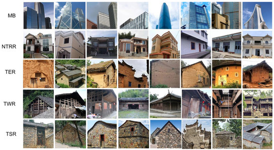
Figure 2.
Illustrative examples of classification categories in the dataset (sourced from Google and field research).
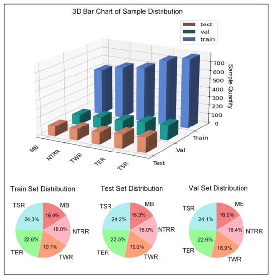
Figure 3.
Visual analysis of sample quantity and proportions in the dataset.
2.2.2. Data Preprocessing
During the data preprocessing stage, normalization, standardization, and data augmentation techniques were primarily applied to optimize model performance. First, the image sizes were standardized to 224 × 224 pixels to maintain consistency in the input data across the subsequent models. To accelerate model convergence and enhance stability, normalization and standardization were performed on the data [39,53]. Data augmentation techniques were then utilized to expand the dataset, thereby improving model robustness and effectively reducing overfitting. Specifically, random cropping and horizontal flipping were applied to enable the model to learn more diverse sample features. Random cropping is a technique that involves randomly selecting different regions from dataset images to simulate various perspectives or framing ranges of buildings within the images, thereby generating more training samples. Horizontal flipping, on the other hand, enhances data diversity by flipping the images horizontally [54]. During the model training phase, transfer learning was introduced, leveraging pretrained models on the ImageNet dataset for parameter transfer. By using parameters trained on a large-scale dataset, transfer learning reduces the dependence on large, annotated datasets for the new task [55,56].
2.2.3. Test Sets
From the initial dataset, a portion was allocated as Test Set 1 to evaluate the model’s performance. To further verify the model’s generalization ability in real-world applications, the research team conducted fieldwork in traditional settlements in Xiangxi, China, selecting Shuangfeng Village, Lahao Village, and Zhushan Village as study sites. These villages were chosen for two primary reasons: first, they represent typical examples of Chinese historical residences with significant cultural heritage value; second, each village has unique architectural characteristics. Zhushan Village is predominantly composed of rammed-earth residences, Shuangfeng Village primarily features wooden structures, and Lahao Village is known for its earthen residences. Additionally, many non-traditional rural residences and modern urban-style buildings from these areas were included in the dataset. Ultimately, Test Set 2 also included five types of buildings: traditional earthen residences, traditional wooden residences, traditional stone residences, non-traditional rural residences, and modern-style buildings. However, due to the better preservation of historical features in the selected traditional villages, the number of non-traditional rural residences (NTRRs) was relatively small. Nevertheless, the overall sample size for each category is comparable to that of Test Set 1, ensuring the reliability and reference value of the research results. Figure 4 illustrates the geographical locations of the villages and provides representative photographs of their typical buildings.
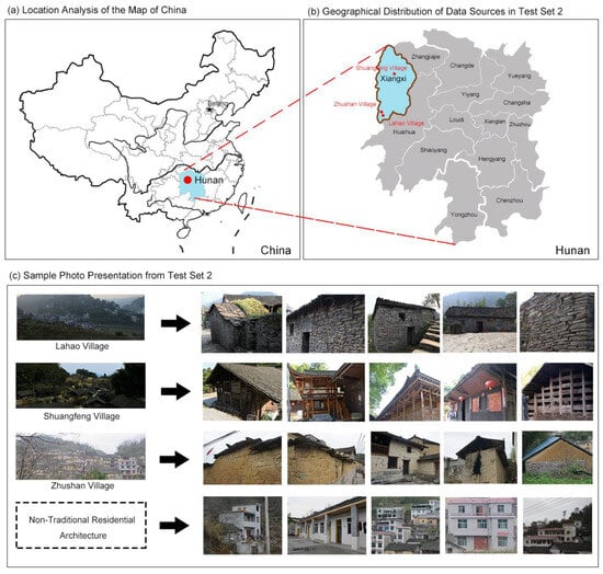
Figure 4.
Spatial distribution and sample images of traditional villages in Test Set 2.
2.2.4. Model Selection
The t-SNE algorithm was applied to the training set for dimensionality reduction, resulting in the two-dimensional scatterplot shown in Figure 5. “Dimension 1” and “Dimension 2” represent the two newly derived feature axes after dimensionality reduction. These two-dimensional coordinates visually illustrate the relative distribution of the five building types (TSR, TER, TWR, NTRR, MB) in the high-dimensional feature space. From the Figure, it can be observed that the data points for the different building types exhibit noticeable overlapping regions in the two-dimensional space. For example, the data points for TSR and TWR show significant overlap, indicating a degree of similarity between these two building types in the high-dimensional feature space. Additionally, some building types, such as TWR and TER, have relatively dispersed distributions with weaker clustering, reflecting greater diversity in these samples during the feature extraction process. This distribution pattern suggests that the five building types do not form entirely distinct boundaries in the classification task, and more complex models may be required to extract more discriminative features to improve classification performance [57].
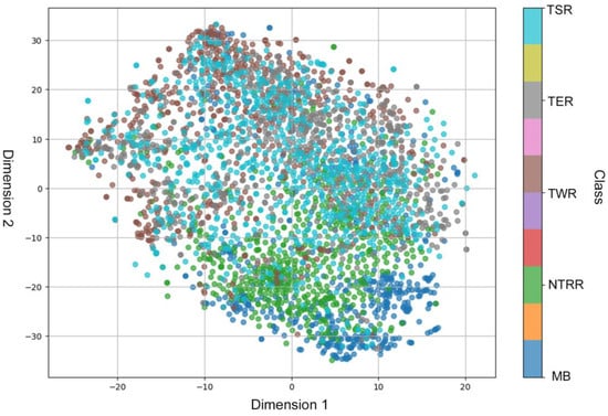
Figure 5.
Dataset clustering analysis using t-SNE (each point in this Figure represents a sample, and its color corresponds to the building type of the sample).
To address this, this paper proposes and implements an improved model that combines the GCSA module with the Swin Transformer structure to deeply extract detailed features and structural information from architectural images (as shown in Figure 6). The input image is a three-channel image with dimensions of C × H × W, where C = 3 represents the number of channels and H and W are the height and width of the image, respectively. The GCSA module first processes the input image through a channel attention sub-module. Specifically, the dimensions of the input feature map are transformed from C × H × W to W × H × C. This is followed by processing through a two-layer Multi-Layer Perceptron (MLP). In the first MLP layer, the number of channels is reduced, and a nonlinear transformation is introduced using the ReLU activation function. The second MLP layer restores the channel dimensions to their original size. The resulting channel attention map is obtained through a Sigmoid activation function and is multiplied element-wise with the original feature map to enhance the channel-specific features of the image. Subsequently, to further enhance the expressive power of the features, the input image undergoes a channel-shuffling operation. The feature map is divided into four groups, and each group is transposed to shuffle the order of the channels within each group. The shuffled feature map is then restored to its original shape of C × H × W. Next, the feature map is passed through a spatial attention sub-module. Here, the feature map undergoes a 7 × 7 convolution layer that reduces the number of channels, followed by batch normalization and ReLU activation. A second 7 × 7 convolution layer restores the channel dimensions to the original size C, and after batch normalization, a spatial attention map is generated using a Sigmoid activation function. Finally, the generated spatial attention map is multiplied element-wise with the shuffled feature map, resulting in the enhanced feature map. Throughout this process, the input image dimensions remain unchanged, and the output feature map retains its dimensions of C × H × W.
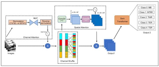
Figure 6.
Transformer Swin–GCSA enhanced architecture.
The enhanced feature map is then fed into the Swin Transformer, which employs a local window attention mechanism and uses a hierarchical structure to progressively capture both global and local information in the image [58]. After processing through multiple Transformer encoders, the feature map is mapped into the classification space and passed through a fully connected layer for five-class classification. The output layer of the Swin Transformer is adjusted to have five output nodes, corresponding to the following five categories: MB, NTRR, TWR, TER, and TSR. Finally, using the Softmax activation function, the model generates the predicted probability for each category. By integrating the GCSA module with the Swin Transformer, the model effectively extracts critical features from images, improving the accuracy and robustness of the classification tasks.
Finally, this model is compared with well-performing classical CNN models (including AlexNet, VGG16, ResNet50, ResNet101, and DenseNet121) to evaluate its training performance and classification effectiveness in building image recognition tasks.
2.2.5. Training Parameters
The experiment was conducted on the deep learning framework PyTorch, using two NVIDIA 4090 GPUs (24GB) for training. PyTorch is an open-source deep learning framework developed by Facebook’s Artificial Intelligence Research (FAIR) lab. It features dynamic computation graph capabilities, enabling the flexible and efficient handling of tensors and deep learning models. In addition to supporting various neural network architectures and excelling in tasks such as computer vision, natural language processing, and reinforcement learning, it integrates seamlessly with CUDA, allowing for GPU-accelerated computations. To ensure that the model converges stably in a short period and achieves optimal performance, the training parameters were carefully designed. First, the batch size was set to 64 to balance memory usage and model convergence speed [59,60]. The learning rate was set to 1 × 10⁻⁴, with a smaller learning rate chosen to prevent gradient oscillation, thereby enhancing model stability and avoiding local minima. Considering the rapid convergence of the model, the number of training epochs was set to 100, ensuring sufficient learning within a reasonable timeframe. CrossEntropyLoss was used as the loss function, which is suitable for multi-class tasks and provides stable gradient signals during training [61]. Additionally, the optimizer selected was AdamW, which combines the Adam algorithm with a weight decay strategy. This combination effectively suppresses unnecessary weight growth over multiple updates, making it well suited for weight management and regularization in deep network training [62].
To systematically evaluate the impact of different parameter settings and preprocessing methods on model performance, several controlled experiments with modified parameters were designed. These included the following: removing data normalization to observe its effect on training performance; eliminating transfer learning to assess the role of pretrained weights; omitting data augmentation to measure the model’s performance when relying solely on raw data; creating a control group without both pretrained weights and data normalization to evaluate performance differences when the model relies entirely on raw data and unoptimized initialization; and adjusting the learning rate from 1 × 10⁻⁴ to 1 × 10⁻³ to explore its impact on training speed and performance.
2.2.6. Evaluation Metrics
In deep learning classification tasks, accuracy is a commonly used evaluation metric, representing the proportion of correctly classified samples. However, due to the complexity of this task, additional metrics were employed to provide a more comprehensive assessment of model performance. These metrics include precision, recall, and F1 score, in addition to accuracy. Precision indicates the proportion of true positive samples among all samples predicted as positive by the model, reflecting the model’s accuracy in identifying positive samples. Recall represents the proportion of true positive samples among all actual positive samples, indicating the model’s ability to recognize positive samples. The F1 score is the harmonic mean of the precision and recall, designed to balance these two metrics and provide an overall evaluation standard [63,64].
The specific formulas are as follows:
(true positive) refers to the number of samples correctly predicted as positive by the model, meaning the samples that are actually positive and successfully recognized as such. (false positive) indicates the number of negative samples incorrectly predicted as positive, meaning samples that are actually negative but mistakenly classified as positive. (false negative) refers to the number of positive samples incorrectly predicted as negative, meaning samples that are actually positive but mistakenly classified as negative. (true negative) represents the number of samples correctly predicted as negative by the model, meaning samples that are actually negative and accurately recognized as such. By comprehensively considering these metrics, it is possible to fully evaluate the performance of deep learning in the recognition and classification tasks of historical buildings, thereby ensuring the model’s effectiveness and reliability in practical applications.
2.2.7. Interpretability Analysis Methods
This study employed interpretability techniques such as feature map visualization, t-SNE dimensionality reduction visualization, and Grad-CAM. Feature maps are generated through convolution operations, where each convolutional kernel (filter) slides over the input image to produce an individual output image. Typically, multiple convolutional kernels exist in a convolutional layer, with each kernel responding to different features of the input image, resulting in multiple feature maps per layer. Each feature map represents the response of the image to a specific convolutional kernel, serving as the layer’s independent output when recognizing particular features, such as edges, textures, or colors. By examining these feature maps, the model’s capability to capture various levels of information in the image can be revealed, aiding in understanding how the model incrementally extracts and processes key features in the image for classification tasks [65].
t-SNE dimensionality reduction visualization is a commonly used nonlinear dimensionality reduction technique widely applied for visualizing high-dimensional data. It projects high-dimensional data points into two- or three-dimensional space, effectively revealing local structures and similarities in the lower-dimensional space. The core idea of t-SNE is to preserve the distance relationships of similar data points in a high-dimensional space, retaining their relative positions as closely as possible in a reduced, low-dimensional space, thereby helping to uncover clustering structures, distribution patterns between categories, and their intrinsic relationships.
Grad-CAM is a gradient-weighted class activation mapping method aimed at visualizing the regions of focus for specific classes in deep learning models. By using Grad-CAM, one can identify the areas of the image that the model prioritizes when making classification decisions, which helps explain the model’s reasoning process. Utilizing these three analytical techniques allows for a deep understanding of feature learning and decision-making processes in deep learning tasks, thus providing critical support for the interpretability of the model [66].
3. Experiment and Results
3.1. Performance of Different Deep Learning Models
We trained several models on the dataset and evaluated them on Test Set 1 and Test Set 2 to comprehensively compare their performance. The models included in this comparison are Transformer Swin–GCSA, AlexNet, DenseNet121, ResNet50, ResNet101, and VGG16. To ensure the reliability of the comparison, all models underwent preprocessing steps such as transfer learning, data augmentation, and normalization, with their parameter settings kept as consistent as possible across models.
Observing the loss value trends in each model during the training process (see Figure 7), it is evident that Transformer Swin–GCSA demonstrated the best performance. The model reached very low loss values almost immediately at the beginning of training, exhibited significantly faster convergence, and maintained stability throughout the training process, showing overall superior performance. In contrast, the remaining CNN models, particularly AlexNet and VGG16, had higher and more fluctuating loss values during training, indicating relatively inferior performance.
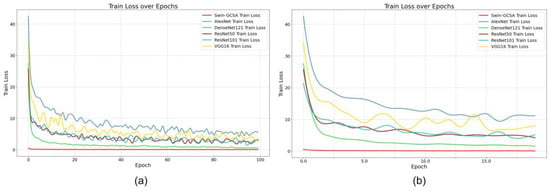
Figure 7.
Model performance in terms of training loss over epochs: (a) shows the training loss over the first 200 epochs, and (b) illustrates the training loss over the first 20 epochs.
A further comparison of accuracy, precision, recall, and F1 score variations across the different models on both the training and validation sets (as shown in Figure 8) reveals that the Transformer Swin–GCSA model demonstrates superior performance during the training process. The model achieves values close to 1.0 for accuracy, precision, recall, and F1 score on both the training and validation sets, indicating its strong generalization capability. ResNet50 and ResNet101 also perform exceptionally well, ranking just below Transformer Swin–GCSA. Although DenseNet121’s performance is slightly lower, it still exhibits a reliable level of accuracy. In contrast, AlexNet and VGG16 show suboptimal performance on the validation set with significant fluctuations and poor generalization.
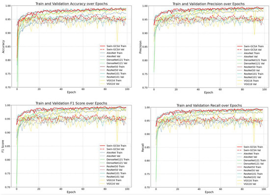
Figure 8.
Performance comparison of deep learning models on accuracy, precision, F1 score, and recall during the training process.
After training completion, the trained weights of each model were applied to Test Set 1 for performance testing and evaluation (see Table 1). The results show that all models demonstrated good classification performance for this task, though differences in performance still existed. The Transformer Swin–GCSA model achieved nearly perfect F1 scores, precisions, and recalls across all categories, with an overall F1 score and accuracy of 0.9784, indicating outstanding performance. Particularly in the MB, NTRR, and TWR categories, the F1 score almost reached 0.99, reflecting its excellent classification and generalization capabilities. However, comparatively, its precision for the NTRR category was 0.95, which was lower than that in other categories and did not demonstrate a significant advantage over the other models.

Table 1.
Performance comparison of deep learning models on Test Set 1.
DenseNet121 also performed well overall, with an F1 score of 0.9682, slightly lower than that of Swin–GCSA. In the MB category, DenseNet121 achieved a recall rate of 1.0, demonstrating an exceptionally high recognition rate for this category. The other models showed comparatively lower performances, with differences of approximately three percentage points between VGG and Transformer Swin–GCSA across various metrics.
Through an analysis of the confusion matrix on Test Set 1 (see Figure 9), the Transformer Swin–GCSA model was shown to demonstrate outstanding classification accuracy, with relatively few misclassifications across the categories. Notably, in the MB, NTRR, and TWR categories, only one sample was incorrectly classified, achieving near-perfect performance. Additionally, the model performed excellently in the TER and TSR categories, effectively distinguishing most samples. In contrast, the other models showed weaker performance in the TSR and TER categories. All CNN models had more than 10 misclassifications in the TSR category, with VGG16 exceeding 20 incorrect classifications. Furthermore, the CNN models also performed relatively poorly in the TER category, especially VGG16 and AlexNet, both of which had over ten misclassifications.
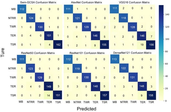
Figure 9.
Comparative analysis of model classification accuracy on Test Set 1 using confusion matrices.
To better assess the generalization capabilities of each model, Test Set 2, collected from traditional settlements, was used to further evaluate the performance of the trained models (see Table 2). The results show that the Transformer Swin–GCSA model maintained excellent performance on Test Set 2, achieving a high overall F1 score (0.9670), precision (0.968), and recall (0.9671), with an overall accuracy of 0.9671. In contrast, the other CNN models exhibited some performance issues. For instance, while VGG16 achieved a precision of 1.0 in the NTRR category, its recall was only 0.8194, indicating a substantial problem with missed detections. ResNet50 also showed a lower recall in the NTRR category, with an F1 score of 0.9022 and recall of 0.8333, indicating similar issues with missed detections. ResNet101 performed even worse, with an F1 score of just 0.8032 and recall of 0.6805, reflecting a high rate of missed detections. DenseNet121’s performance in the NTRR category was also suboptimal, with an F1 score of 0.7627 and recall of only 0.6250, indicating significant issues with missed detections. Additionally, in the TER category, DenseNet121 achieved an F1 score of 0.9176 with a high recall but low precision; in the TSR category, its F1 score was 0.9236, but precision remained low. For AlexNet, in the NTRR category, the F1 score was 0.9037, with a precision of 0.9682 and recall of 0.8472, indicating issues with missed detections. In the TSR category, AlexNet achieved an F1 score of 0.9461 with a recall of 0.9840, but its precision was lower (0.9111), suggesting a higher rate of false positives. In summary, in terms of overall performance and recognition across most categories, Transformer Swin–GCSA remained the best-performing model. However, its performance in the NTRR category was relatively less advantageous. By comparison, VGG16 achieved a precision of 1.0 in the NTRR category, while DenseNet121 achieved a precision of 0.97, both of which were higher than that of Transformer Swin–GCSA.
Table 2.
Performance comparison of deep learning models on Test Set 2.
The superiority of Transformer Swin–GCSA is also evident from the confusion matrix on Test Set 2 (see Figure 10). Although it recorded six misclassifications in the TER category, slightly lagging behind some of the CNN models, its overall performance remains outstanding, especially in the NTRR category where it demonstrated a high discriminative capability. The NTRR category was particularly challenging, with CNN models showing relatively low classification accuracies in this category. For instance, in the NTRR category, AlexNet misclassified 11 samples, VGG16 misclassified 13, ResNet50 misclassified 12, ResNet101 misclassified as many as 23, and DenseNet121 misclassified 27 samples.
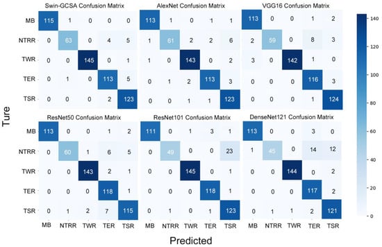
Figure 10.
Comparative analysis of model classification accuracy on Test Set 2 using confusion matrices.
3.2. Impact of Different Training Strategies and Parameters on Model Performance
To further investigate the impact of various parameter settings and deep learning strategies on the task of historical building recognition and classification, this study employed the best-performing Swin–GCSA model for testing, with multiple control groups set up in comparison to the standard settings group. The control settings included the following: removing data normalization, eliminating transfer learning, excluding data augmentation, using a control group without pretrained weights and data normalization, and adjusting the learning rate from 1 × 10⁻⁴ to 1 × 10⁻³. Each control group was trained separately, and from the trend in loss values during training (see Figure 11), it can be observed that the standard training group showed the fastest loss reduction, stabilizing within 10 epochs and reaching the lowest level early in the process, maintaining a low loss throughout training. After adjusting the learning rate, the loss reduction speed remained fast, nearly on par with the standard training group, reaching a low level in the early stages but showing slight fluctuations at certain points. In contrast, other control groups exhibited slower loss reduction with greater fluctuations, particularly the “no normalization” control group, which had the poorest training results, with large fluctuations and the highest final stabilized loss. These results indicate that parameters and strategies such as data augmentation, normalization, pretrained weights, and an appropriate learning rate positively contribute to enhancing training performance.
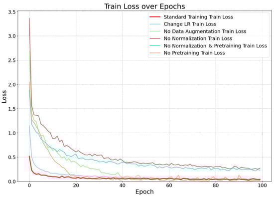
Figure 11.
Loss trend under different training strategies.
A further comparison of the performance of the standard group and each control group on metrics such as accuracy, precision, F1 score, and recall during training (see Figure 12) revealed that the standard group outperformed all control groups across all metrics, with training and validation accuracy both approaching 1.0 and showing minimal difference, indicating no overfitting. Additionally, the training process for the standard group was stable, with no significant fluctuations and a faster convergence rate. In contrast, the control group with the adjusted learning rate also performed well, with metrics slightly lower than those of the standard group. The other control groups showed slower convergence rates, larger fluctuations, and relatively lower values for both the training and validation metrics. These results indicate that data augmentation, normalization, pretraining, and appropriate learning rate adjustment collectively improved the model’s classification performance and generalization ability.
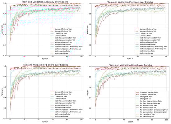
Figure 12.
Performance comparison of training data under parameter variations.
After training, the trained models were applied to the test set for evaluation. The results on Test Set 1 (see Table 3) show that the standard model performed excellently across all categories, achieving the highest overall F1 score (0.9784), precision (0.9787), and recall (0.9784). The model with an adjusted learning rate had an overall F1 score of 0.9726, slightly lower than the standard model but still performing well overall. In contrast, the model without pretraining had a significantly lower overall F1 score of 0.9215, performing poorly in multiple categories, especially in the TSR category, where the recall was only 0.8333 and the F1 score was low (0.9034 in the TER category and 0.8860 in the TSR category), indicating weaker performance in the TSR category. The model without data augmentation had an overall F1 score of 0.8577, notably lower than the standard model, with declines in all categories, especially in the MB category, where the recall dropped to only 0.7787. The models without normalization and with neither normalization nor pretraining performed extremely poorly, almost failing to achieve effective classification, with most metrics falling below 0.25, indicating severe overfitting. In summary, the model without normalization exhibited significant declines across all categories, underscoring the crucial role of normalization for model training effectiveness and stability. Adjusting the learning rate had the least impact on model performance, while pretraining and data augmentation also contributed significantly to improvements in training and testing performance.
Table 3.
Evaluation of model performance with varying parameters and strategies.
3.3. Interpretability Study
To investigate the interpretability of the deep learning model and explore its “black-box” characteristics, techniques such as t-SNE dimensionality reduction analysis, feature map and heatmap analysis, and Grad-CAM were employed to dissect the model’s prediction process. The aim was to gain a deep understanding of how the model extracts key information from the raw input and performs reasoning, revealing potential biases and limitations in its decision-making process, thereby providing a theoretical foundation for further optimizing model performance and enhancing its trustworthiness and interpretability.
By using the t-SNE algorithm for the two-dimensional visualization of features learned by the Transformer Swin–GCSA model (see Figure 13), high-dimensional data were mapped to a two-dimensional space to analyze the distribution of the dataset in a lower-dimensional space. The results show that the samples from each category formed clear clusters in the two-dimensional space, indicating good separability between the classes. This suggests that the Transformer Swin–GCSA model successfully learned features that can be effectively distinguished between categories during training. Among them, the MB and TSR categories were clustered far apart, indicating significant feature differences between these two classes, whereas the TER and TSR clusters were relatively close, suggesting similar features between them, though still distinctly separable. Additionally, the TSR category was located in the center of the feature space, possibly reflecting certain similarities or overlaps with other categories’ features.
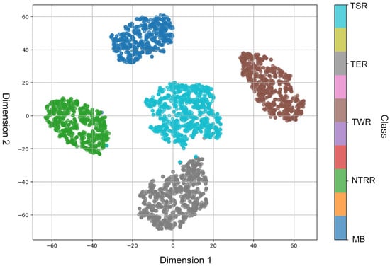
Figure 13.
t-SNE projection of Transformer Swin–GCSA model in the dataset.
The heatmaps generated using Grad-CAM visualize the focus areas of the Swin–GCSA model when classifying different building types (MB, NTRR, TER, TWR, TSR) (as shown in Figure 14). In the images of modern buildings (MBs), the model primarily focuses on the building contours, height, and lines, particularly emphasizing facades, windows, and vertical structures, indicating the importance of these regions in identifying this category. In the heatmaps for the TER category, the model’s attention is concentrated on the roof, walls, and edges, areas that typically reflect the characteristic structural features of traditional earthen buildings. For the TWR category, the heatmap shows that the model is focused on the texture and structural details of the walls, especially the texture and material of wooden structures. In the TSR category, the model’s attention is focused on stone walls, structural edges, and textural details, highlighting its ability to recognize features specific to this category. In the NTRR category, the model shows a high level of attention to windows, eaves, and exterior walls, indicating that it relies on these architectural details for classification.
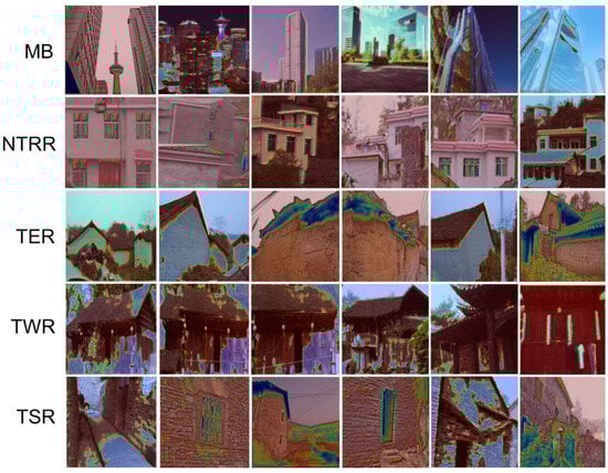
Figure 14.
Visualization of Grad-CAM heatmaps for different building types.
To illustrate the Transformer Swin–GCSA model’s focus at different hierarchical levels, an analysis was conducted on the feature maps and heatmap overlays extracted from various convolutional layers using an image of a traditional stone residence from the dataset (see Figure 15). In the first layer’s heatmap overlay, the model’s highlighted areas are concentrated on the overall structure of the building, especially the wall sections. In the second layer, the model’s focus shifts more specifically to certain structural features of the building, such as the roof outline, with attention becoming more concentrated compared to the first layer. By the third layer, the heatmap shows a further refinement of attention, zeroing in on specific structural details like roof textures and other fine-grained features. The feature maps from each layer illustrate the convolutional filters’ focus at different depths, reflecting this hierarchical progression. In the first layer, the feature maps capture the basic structure of the image, with the model primarily focusing on large areas such as the building’s walls. The second layer’s feature maps begin to reveal more local structures and shapes, such as the outline of the roof. In the third layer, the feature maps become more abstract, starting to capture material and textural characteristics; some feature maps even highlight the textures of stone walls or specific roof structures.
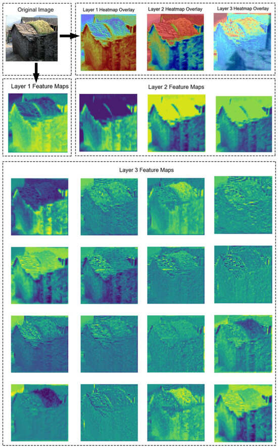
Figure 15.
Heatmap and feature map analysis in Transformer Swin–GCSA model.
This progressive feature extraction process, from the building’s overall wall structure at the initial layer to the outline of the roof at the mid-layer, and finally to the material and texture details at the upper layer, demonstrates the effectiveness of the Transformer Swin–GCSA model’s hierarchical learning strategy. This stepwise approach to understanding the image enables the model to make an accurate classification by gradually constructing a detailed comprehension of the category.
4. Discussion
This study constructs a historical architecture dataset and develops a deep learning model based on the Swin Transformer-GCSA framework, incorporating advanced regularization and data augmentation techniques. The model achieves the high-precision classification and detailed feature recognition of Chinese historical architecture images, providing a robust technical foundation for the digital modeling and damage assessment of historical buildings. These advancements facilitate the formulation of precise restoration strategies and contribute to the establishment of regional historical architecture databases, thereby offering a scientific basis for governmental and cultural heritage institutions to prioritize conservation efforts and formulate region-specific policies.
4.1. Model Performance and Innovations
The Swin Transformer-based model with the GCSA proposed in this study demonstrated notable accuracy in the classification tasks for historical architecture images. Compared to other classification and recognition tasks in the architectural field, this model showed superior performance in metrics such as accuracy [29,67]. The introduction of the GCSA mechanism significantly enhanced the model’s feature extraction capability for architectural images, particularly in capturing both detailed and global information. It enabled a more effective integration of local and global features. The experimental results indicated that complex models performed better on historical architecture datasets. For instance, the complex Transformer-based Swin–GCSA model exhibited optimal performance across various evaluation metrics, whereas relatively complex CNN architectures like DenseNet121, ResNet101, and ResNet50 still outperformed simpler models such as VGG16 and AlexNet in certain classification and recognition tasks. In addition, our model was optimized through various measures such as data augmentation and pretraining, while two different test sets were introduced to minimize the potential impact of insufficient sample size. The experimental results indicated that the model did not exhibit overfitting during the training and testing phases, demonstrating that the current sample size and distribution are reasonable and feasible for this study.
From the perspective of parameter tuning and strategy optimization, normalization significantly impacted the training process. Omitting the normalization step led to overfitting, making classification and recognition on the test set nearly unachievable. Pretrained models and data augmentation strategies considerably accelerated the convergence rate during training and improved test set performance. Adjusting the learning rate within a specific small range had a minimal impact on the test results.
Furthermore, an analysis of the confusion matrices for Test Set 1 and Test Set 2 using the Swin Transformer revealed the following patterns: in Test Set 1, TER and TSR were the most frequently misclassified categories, whereas in Test Set 2, NTRR and TER showed higher misclassification rates. This indicates that the model demonstrates higher accuracy in distinguishing between modern and non-modern buildings but performs slightly worse in certain non-modern categories, especially those with similar material characteristics. Additionally, the prediction performance for the same category may vary across different datasets.
4.2. Interpretability Analysis
Previous studies often used Grad-CAM as their primary interpretability tool. However, this study integrates feature maps, t-SNE dimensionality reduction, and Grad-CAM, demonstrating the advantages of this combined approach in understanding the model’s decision-making process [1]. Compared to a single method, this integrated approach not only clearly identifies the key areas of the model’s focus but also reveals how the model gradually extracts features from a low level to a high level. Using t-SNE for dimensionality reduction further enables the observation of the distribution of different categories of architectural samples in the feature space, thereby verifying the model’s classification effectiveness. This integrated approach enhances the transparency of the model’s behavior and reveals its decision-making mechanisms from multiple perspectives. The experimental results indicate that the step-by-step feature extraction process is similar to human visual cognition, initially recognizing the overall image, then further identifying and extracting through details and textures.
4.3. Limitations and Future Prospects
One limitation of this study lies in the diversity of the dataset, which still requires further enhancement. While the model demonstrates strong performance in identifying the traditional features and material types of Chinese historical architecture, as well as in distinguishing between rural and modern buildings, its application is largely focused on Chinese historical heritage and has not been extended to architectural styles from other countries. Additionally, the dataset lacks comprehensive annotations for specific architectural details, such as the number of floors, window and door styles, and facade components. This limitation may restrict the model’s application scope and generalization ability to a certain extent.
Although the Transformer-based Swin–GCSA model demonstrates superior performance compared to traditional CNN models in many tasks, its performance can be inconsistent when handling certain specific types, such as NTRR. This may be attributed to the Transformer model’s emphasis on global feature extraction, which can result in limitations in capturing critical, discriminative local details. Therefore, exploring models better suited for the recognition of historical architectural images remains a topic worth in-depth investigation. For instance, studying alternative forms of Transformer modules or integrating CNNs with different attention mechanisms or feature enhancement modules may further improve recognition performance. The applicability and potential advantages of these novel models require comprehensive validation and evaluation through future research.
Given these limitations, future research will focus on expanding the scale and geographical coverage of the historical building datasets, incorporating a wider range of architectural features while exploring more advanced model architectures. These efforts aim to enhance the model’s ability to recognize various types of buildings, enable effective performance in complex scenarios, and support the comparative analysis of historical architectural heritage across different countries, thereby providing deeper insights into architectural features within diverse cultural contexts.
5. Conclusions
In the context of rapid advancements in geographic information technology and artificial intelligence, challenges such as the difficulty of digital information collection for certain historical buildings and districts, low data quality, inefficiencies in manual classification, and the limitations of traditional models in handling historical architecture datasets have become prominent. This study addresses these issues by constructing a high-quality dataset specifically for historical Chinese architecture through a combination of field surveys, Internet resource collection, and manual annotation. Additionally, two test sets were developed to validate model performance. Based on this dataset, a deep learning model incorporating the Swin Transformer and GCSA mechanism was proposed. Compared to a classic CNN, this model demonstrated significant superiority in training and testing, achieving optimal results in historical building classification tasks. In Test Set 1, the model achieved over 0.978 in its accuracy, precision, recall, and F1 score, demonstrating exceptionally high classification performance. A further evaluation on Test Set 2, which included real-world historical architecture from traditional settlements, showed that all metrics remained above 0.967, highlighting the model’s robustness and effectiveness in complex environments.
Moreover, this study explored the impact of various parameter settings and preprocessing methods on model performance. The results indicated that an absence of standardization led to severe overfitting, causing significant declines in performance metrics, with accuracy and other indicators dropping to nearly 0.24, rendering the model ineffective in classification tasks. Without pretraining or data augmentation strategies, the model’s convergence rate noticeably slowed, and its performance on the test sets declined by 5% to 12%. Regarding learning rate adjustments, it was found that as long as the learning rate was maintained within a reasonable range, variations had a minimal effect on model performance. To further enhance interpretability, this study applied integrated methods such as Grad-CAM, feature maps, and t-SNE dimensionality reduction to conduct a comprehensive interpretability analysis of the model. The results revealed that the Swin–GCSA model could progressively extract multi-layered features from architectural images, focusing on overall structure, roof contours, and material textures in successive layers. In the classification of different architectural types, the model was able to concentrate on specific structural characteristics, enabling the accurate classification of historical architecture images.
The findings of this study provide valuable insights into expansion strategies for digital information related to historical architectural heritage. This approach enables researchers to accurately identify whether a building aligns with traditional aesthetics, gain a deeper understanding of its material properties, and effectively distinguish between modern and rural architectural features. Moreover, it facilitates the development of precise restoration strategies and supports the establishment of regional historical architecture databases, thereby providing scientific guidance for governments and cultural heritage institutions in prioritizing conservation efforts and formulating region-specific protection policies.
Author Contributions
J.W. designed and conducted the study, analyzed the data, prepared the figures, and wrote the manuscript. Y.Y. supervised the work. Y.T. and Z.L. revised the manuscript. All authors have read and agreed to the published version of the manuscript.
Funding
This research is funded by the National Key Research and Development Program of China, titled “Integration and Comprehensive Demonstration of Low-carbon Ecological Rural Community Intelligent Construction Technologies” (Project No. 2024YFD1600405). Additionally, it is supported by the project “Research on Key Technologies for Integrated Digital Contextual Architecture with Design-Build Synergy in Multidimensional Positive BIM” (Grant No. cscec5b-2023-01). Furthermore, the research is funded by the project “Coupling Research and Application Demonstration of Zero-Energy Building Construction and Carbon-Free Operation Technology Based on Recycled Materials” (Grant No. CSCEC-2023-Z-01).
Data Availability Statement
All data were generated by the authors’ field collection and software simulation.
Conflicts of Interest
Authors Yang Ying, Yigao Tan and Zhuliang Liu were employed by the company China Construction Fifth Engineering Division Co., Ltd. The remaining author declares that the research was conducted in the absence of any commercial or financial relationships that could be construed as a potential conflict of interest.
References
- Zhao, X.; Lu, Y.; Lin, G. An integrated deep learning approach for assessing the visual qualities of built environments utilizing street view images. Eng. Appl. Artif. Intell. 2024, 130, 107805. [Google Scholar] [CrossRef]
- Cao, Y.; Yang, P.; Xu, M.; Li, M.; Li, Y.; Guo, R. A novel method of urban landscape perception based on biological vision process. Landsc. Urban Plan. 2025, 254, 105246. [Google Scholar] [CrossRef]
- Li, W.; Sun, R.; He, H.; Chen, L. How does three-dimensional landscape pattern affect urban residents’ sentiments. Cities 2023, 143, 104619. [Google Scholar] [CrossRef]
- Dang, X.; Liu, W.; Hong, Q.; Wang, Y.; Chen, X. Digital twin applications on cultural world heritage sites in China: A state-of-the-art overview. J. Cult. Herit. 2023, 64, 228–243. [Google Scholar] [CrossRef]
- Ogawa, Y.; Oki, T.; Zhao, C.; Sekimoto, Y.; Shimizu, C. Evaluating the subjective perceptions of streetscapes using street-view images. Landsc. Urban Plan. 2024, 247, 105073. [Google Scholar] [CrossRef]
- Shin, H.-S.; Woo, A. Analyzing the effects of walkable environments on nearby commercial property values based on deep learning approaches. Cities 2024, 144, 104628. [Google Scholar] [CrossRef]
- Ramalingam, S.P.; Kumar, V. Building usage prediction in complex urban scenes by fusing text and facade features from street view images using deep learning. Build. Environ. 2025, 267, 112174. [Google Scholar] [CrossRef]
- Gara, F.; Nicoletti, V.; Arezzo, D.; Cipriani, L.; Leoni, G. Model Updating of Cultural Heritage Buildings Through Swarm Intelligence Algorithms. Int. J. Archit. Herit. 2023, 11, 1–17. [Google Scholar] [CrossRef]
- Ito, K.; Bansal, P.; Biljecki, F. Examining the causal impacts of the built environment on cycling activities using time-series street view imagery. Transp. Res. Part A Policy Pract. 2024, 190, 104286. [Google Scholar] [CrossRef]
- Tarkhan, N.; Szcześniak, J.T.; Reinhart, C. Façade feature extraction for urban performance assessments: Evaluating algorithm applicability across diverse building morphologies. Sustain. Cities Soc. 2024, 105, 105280. [Google Scholar] [CrossRef]
- Larkin, A.; Gu, X.; Chen, L.; Hystad, P. Predicting perceptions of the built environment using GIS, satellite and street view image approaches. Landsc. Urban Plan. 2021, 216, 104257. [Google Scholar] [CrossRef] [PubMed]
- Kim, J.; Park, J.; Lee, J.; Jang, K.M. Examining the socio-spatial patterns of bus shelters with deep learning analysis of street-view images: A case study of 20 cities in the U.S. Cities 2024, 148, 104852. [Google Scholar] [CrossRef]
- Sun, M.; Zhang, F.; Duarte, F.; Ratti, C. Understanding architecture age and style through deep learning. Cities 2022, 128, 103787. [Google Scholar] [CrossRef]
- Liang, X.; Chang, J.H.; Gao, S.; Zhao, T.; Biljecki, F. Evaluating human perception of building exteriors using street view imagery. Build. Environ. 2024, 263, 111875. [Google Scholar] [CrossRef]
- Sánchez, I.A.V.; Labib, S.M. Accessing eye-level greenness visibility from open-source street view images: A methodological development and implementation in multi-city and multi-country contexts. Sustain. Cities Soc. 2024, 103, 105262. [Google Scholar] [CrossRef]
- Xiang, H.; Xie, M.; Huang, Z.; Bao, Y. Study on spatial distribution and connectivity of Tusi sites based on quantitative analysis. Ain Shams Eng. J. 2023, 14, 101833. [Google Scholar] [CrossRef]
- Xie, L.; Li, Z.; Li, J.; Yang, G.; Jiang, J.; Liu, Z.; Tong, S. The Impact of Traditional Raw Earth Dwellings’ Envelope Retrofitting on Energy Saving: A Case Study from Zhushan Village, in West of Hunan, China. Atmosphere 2022, 13, 1537. [Google Scholar] [CrossRef]
- Rocco, A.; Vicente, R.; Rodrigues, H.; Ferreira, V. Adobe Blocks Reinforced with Vegetal Fibres: Mechanical and Thermal Characterisation. Buildings 2024, 14, 2582. [Google Scholar] [CrossRef]
- Ferretto, P.W.; Cai, L. Village prototypes: A survival strategy for Chinese minority rural villages. J. Archit. 2020, 25, 1–23. [Google Scholar] [CrossRef]
- Bian, J.; Chen, W.; Zeng, J. Spatial Distribution Characteristics and Influencing Factors of Traditional Villages in China. Int. J. Environ. Res. Public Health 2022, 19, 4627. [Google Scholar] [CrossRef]
- Wang, F.; Yu, F.; Zhu, X.; Pan, X.; Sun, R.; Cai, H. Disappearing gradually and unconsciously in rural China: Research on the sunken courtyard and the reasons for change in Shanxian County, Henan Province. J. Rural. Stud. 2016, 47, 630–649. [Google Scholar] [CrossRef]
- Lin, L.; Du, C.; Yao, Y.; Gui, Y. Dynamic influencing mechanism of traditional settlements experiencing urbanization: A case study of Chengzi Village. J. Clean. Prod. 2021, 320, 128462. [Google Scholar] [CrossRef]
- Ljubenov, G.; Roter-Blagojević, M. Disappearance of the traditional architecture: The key study of Stara Planina villages. SAJ Serbian Archit. J. 2016, 8, 43–58. [Google Scholar] [CrossRef]
- Hu, D.; Zhou, S.; Chen, Z.; Gu, L. Effect of Traditional Chinese Village policy under the background of rapid urbanization in China: Taking Jiangxi Province as an example. Prog. Geogr. 2021, 40, 104–113. [Google Scholar] [CrossRef]
- Hecht, R.; Meinel, G.; Buchroithner, M. Automatic identification of building types based on topographic databases—A comparison of different data sources. Int. J. Cartogr. 2025, 1, 18–31. [Google Scholar] [CrossRef]
- Xiao, C.; Xie, X.; Zhang, L.; Xue, B. Efficient Building Category Classification with Façade Information from Oblique Aerial Images. Int. Arch. Photogramm. Remote Sens. Spat. Inf. Sci. 2020, XLIII-B2-2020, 1309–1313. [Google Scholar] [CrossRef]
- Lin, H.; Huang, L.; Chen, Y.; Zheng, L.; Huang, M.; Chen, Y. Research on the Application of CGAN in the Design of Historic Building Facades in Urban Renewal—Taking Fujian Putian Historic Districts as an Example. Buildings 2023, 13, 1478. [Google Scholar] [CrossRef]
- Gu, J.; Xie, Z.; Zhang, J.; He, X. Advances in Rapid Damage Identification Methods for Post-Disaster Regional Buildings Based on Remote Sensing Images: A Survey. Buildings 2024, 14, 898. [Google Scholar] [CrossRef]
- Han, Q.; Yin, C.; Deng, Y.; Liu, P. Towards Classification of Architectural Styles of Chinese Traditional Settlements Using Deep Learning: A Dataset, a New Framework, and Its Interpretability. Remote Sens. 2022, 14, 5250. [Google Scholar] [CrossRef]
- Gonzalez, D.; Rueda-Plata, D.; Acevedo, A.B.; Duque, J.C.; Ramos-Pollán, R.; Betancourt, A.; García, S. Automatic detection of building typology using deep learning methods on street level images. Build. Environ. 2020, 177, 106805. [Google Scholar] [CrossRef]
- Roussel, R.; Jacoby, S.; Asadipour, A. Robust Building Identification from Street Views Using Deep Convolutional Neural Networks. Buildings 2024, 14, 578. [Google Scholar] [CrossRef]
- Dai, M.; Ward, W.O.C.; Meyers, G.; Tingley, D.D.; Mayfield, M. Residential building facade segmentation in the urban environment. Build. Environ. 2021, 199, 107921. [Google Scholar] [CrossRef]
- Kim, J.; Nguyen, A.-D.; Lee, S. Deep CNN-Based Blind Image Quality Predictor. IEEE Trans. Neural Netw. Learn. Syst. 2019, 30, 11–24. [Google Scholar] [CrossRef] [PubMed]
- Tian, C.; Xu, Y.; Li, Z.; Zuo, W.; Fei, L.; Liu, H. Attention-guided CNN for image denoising. Neural Netw. 2020, 124, 117–129. [Google Scholar] [CrossRef]
- Xiang, C.; Yin, D.; Song, F.; Yu, Z.; Jian, X.; Gong, H. A Fast and Robust Safety Helmet Network Based on a Mutilscale Swin Transformer. Buildings 2024, 14, 688. [Google Scholar] [CrossRef]
- Girard, L.; Roy, V.; Eude, T.; Giguère, P. Swin transformer for hyperspectral rare sub-pixel target detection. In Algorithms, Technologies, and Applications for Multispectral and Hyperspectral Imaging XXVIII; Messinger, D.W., Velez-Reyes, M., Eds.; SPIE: Cergy Pontoise, France, 2022; Volume 5, p. 31. [Google Scholar] [CrossRef]
- Rasmussen, C.B.; Kirk, K.; Moeslund, T.B. The Challenge of Data Annotation in Deep Learning—A Case Study on Whole Plant Corn Silage. Sensors 2022, 22, 1596. [Google Scholar] [CrossRef]
- Božič, J.; Tabernik, D.; Skočaj, D. Mixed supervision for surface-defect detection: From weakly to fully supervised learning. Comput. Ind. 2021, 129, 103459. [Google Scholar] [CrossRef]
- Shorten, C.; Khoshgoftaar, T.M. A survey on Image Data Augmentation for Deep Learning. J. Big Data 2019, 6, 60. [Google Scholar] [CrossRef]
- Kim, S.; Choi, Y.; Lee, M. Deep learning with support vector data description. Neurocomputing 2015, 165, 111–117. [Google Scholar] [CrossRef]
- Li, Q.; Yan, M.; Xu, J. Optimizing Convolutional Neural Network Performance by Mitigating Underfitting and Overfitting. In Proceedings of the 2021 IEEE/ACIS 19th International Conference on Computer and Information Science (ICIS), Shanghai, China, 23–25 June 2021; IEEE: New York, NY, USA, 2021; Volume 6, pp. 126–131. [Google Scholar] [CrossRef]
- Qi, W.; Huang, C.; Wang, Y.; Zhang, X.; Sun, W.; Zhang, L. Global—Local 3-D Convolutional Transformer Network for Hyperspectral Image Classification. IEEE Trans. Geosci. Remote Sens. 2020, 61, 5510820. [Google Scholar] [CrossRef]
- Guo, X.; Meng, L.; Mei, L.; Weng, Y.; Tong, H. Multi-focus image fusion with Siamese self-attention network. IET Image Process. 2020, 14, 1339–1346. [Google Scholar] [CrossRef]
- Qi, M.; Liu, L.; Zhuang, S.; Liu, Y.; Li, K.; Yang, Y.; Li, X. FTC-Net: Fusion of Transformer and CNN Features for Infrared Small Target Detection. IEEE J. Sel. Top. Appl. Earth Obs. Remote Sens. 2022, 15, 8613–8623. [Google Scholar] [CrossRef]
- Khan, S.; Naseer, M.; Hayat, M.; Zamir, S.W.; Khan, F.S.; Shah, M. Transformers in Vision: A Survey. ACM Comput. Surv. 2022, 54, 1–41. [Google Scholar] [CrossRef]
- Zhang, Q.; Xu, Y.; Zhang, J.; Tao, D. ViTAEv2: Vision Transformer Advanced by Exploring Inductive Bias for Image Recognition and Beyond. Int. J. Comput. Vis. 2023, 131, 1141–1162. [Google Scholar] [CrossRef]
- Kim, S.; Nam, J.; Ko, B.C. Facial Expression Recognition Based on Squeeze Vision Transformer. Sensors 2022, 22, 3729. [Google Scholar] [CrossRef]
- Martín, A.; Vargas, V.M.; Gutiérrez, P.A.; Camacho, D.; Hervás-Martínez, C. Optimising Convolutional Neural Networks using a Hybrid Statistically-Driven Coral Reef Optimisation Algorithm. Appl. Soft Comput. 2020, 90, 106144. [Google Scholar] [CrossRef]
- Tian, Q.; Arbel, T.; Clark, J.J. Task dependent deep LDA pruning of neural networks. Comput. Vis. Image Underst. 2021, 203, 103154. [Google Scholar] [CrossRef]
- Jin, X.; Lan, C.; Zeng, W.; Chen, Z. Style Normalization and Restitution for Domain Generalization and Adaptation. In Proceedings of the IEEE Conference on Computer Vision and Pattern Recognition (CVPR), Honolulu, HI, USA, 21–26 July 2017; IEEE: New York, NY, USA, 2017; pp. 975–983. [Google Scholar] [CrossRef]
- Dong, Y.; Su, H.; Zhu, J.; Zhang, B. Improving Interpretability of Deep Neural Networks with Semantic Information. In Proceedings of the 2017 IEEE Conference on Computer Vision and Pattern Recognition (CVPR), Honolulu, HI, USA, 21–26 July 2017; IEEE: New York, NY, USA, 2017; Volume 7, pp. 975–983. [Google Scholar] [CrossRef]
- Liu, Z.; Xu, F. Interpretable neural networks: Principles and applications. Front. Artif. Intell. 2023, 6, 974295. [Google Scholar] [CrossRef]
- Owen, C.A.; Dick, G.; Whigham, P.A. Standardization and Data Augmentation in Genetic Programming. IEEE Trans. Evol. Comput. 2022, 26, 1596–1608. [Google Scholar] [CrossRef]
- Moreno-Barea, F.J.; Jerez, J.M.; Franco, L. Improving classification accuracy using data augmentation on small data sets. Expert Syst. Appl. 2020, 161, 113696. [Google Scholar] [CrossRef]
- Werner, J.M.; O’Leary-Kelly, A.M.; Baldwin, T.T.; Wexley, K.N. Augmenting behavior-modeling training: Testing the effects of pre- and post-training interventions. Hum. Resour. Dev. Q. 1994, 5, 169–183. [Google Scholar] [CrossRef]
- Cannon-Bowers, J.A.; Rhodenizer, L.; Salas, E.; Bowers, C.A. A Framework for Understanding Pre-Practice Conditions and Their Impact on Learning. Pers. Psychol. 1998, 51, 291–320. [Google Scholar] [CrossRef]
- Kimura, M. Generalized t-SNE Through the Lens of Information Geometry. IEEE Access 2021, 9, 129619–129625. [Google Scholar] [CrossRef]
- Liu, Z.; Lin, Y.; Cao, Y.; Hu, H.; Wei, Y.; Zhang, Z.; Lin, S.; Guo, B. Swin transformer: Hierarchical Vision Transformer Using Shifted Windows. In Proceedings of the IEEE/CVF International Conference on Computer Vision, Montreal, BC, Canada, 11–17 October 2021; IEEE: New York, NY, USA, 2021; pp. 10012–10022. [Google Scholar]
- Lin, R. Analysis on the Selection of the Appropriate Batch Size in CNN Neural Network. In Proceedings of the 2022 International Conference on Machine Learning and Knowledge Engineering (MLKE), Guilin, China, 25–27 February 2022; IEEE: New York, NY, USA, 2022; pp. 106–109. [Google Scholar] [CrossRef]
- Choi, M. An Empirical Study on the Optimal Batch Size for the Deep Q-Network. In Proceedings of the Robot Intelligence Technology and Applications 5: Results from the 5th International Conference on Robot Intelligence Technology and Applications, Daejeon, Korea, 13–15 December 2017; Springer: Berlin/Heidelberg, Germany, 2019; pp. 73–81. [Google Scholar]
- Morchdi, C.; Zhou, Y.; Ding, J.; Wang, B. Exploring Gradient Oscillation in Deep Neural Network Training. In Proceedings of the 2023 59th Annual Allerton Conference on Communication, Control, and Computing (Allerton), Monticello, IL, USA, 26–29 September 2023; IEEE: New York, NY, USA, 2023; Volume 9, pp. 1–7. [Google Scholar] [CrossRef]
- Jia, X.; Feng, X.; Yong, H.; Meng, D. Weight Decay with Tailored Adam on Scale-Invariant Weights for Better Generalization. IEEE Trans. Neural Netw. Learn. Syst. 2024, 35, 6936–6947. [Google Scholar] [CrossRef]
- Pezoulas, V.C.; Kourou, K.D.; Kalatzis, F.; Exarchos, T.P.; Venetsanopoulou, A.; Zampeli, E.; Gandolfo, S.; Skopouli, F.; De Vita, S.; Tzioufas, A.G.; et al. Medical data quality assessment: On the development of an automated framework for medical data curation. Comput. Biol. Med. 2019, 107, 270–283. [Google Scholar] [CrossRef]
- Saito, T.; Rehmsmeier, M. The Precision-Recall Plot Is More Informative than the ROC Plot When Evaluating Binary Classifiers on Imbalanced Datasets. PLoS ONE 2015, 10, e0118432. [Google Scholar] [CrossRef]
- Athawale, T.M.; Triana, B.; Kotha, T.; Pugmire, D.; Rosen, P. A Comparative Study of the Perceptual Sensitivity of Topological Visualizations to Feature Variations. IEEE Trans. Vis. Comput. Graph. 2024, 30, 1074–1084. [Google Scholar] [CrossRef]
- Selvaraju, R.R.; Cogswell, M.; Das, A.; Vedantam, R.; Parikh, D.; Batra, D. Grad-CAM: Visual Explanations from Deep Networks via Gradient-Based Localization. In Proceedings of the 2017 IEEE International Conference on Computer Vision (ICCV), Venice, Italy, 22–29 October 2017; IEEE: New York, NY, USA, 2017; Volume 10, pp. 618–626. [Google Scholar] [CrossRef]
- Ramalingam, S.P.; Kumar, V. Automatizing the generation of building usage maps from geotagged street view images using deep learning. Build. Environ. 2023, 235, 110215. [Google Scholar] [CrossRef]
Disclaimer/Publisher’s Note: The statements, opinions and data contained in all publications are solely those of the individual author(s) and contributor(s) and not of MDPI and/or the editor(s). MDPI and/or the editor(s) disclaim responsibility for any injury to people or property resulting from any ideas, methods, instructions or products referred to in the content. |
© 2025 by the authors. Licensee MDPI, Basel, Switzerland. This article is an open access article distributed under the terms and conditions of the Creative Commons Attribution (CC BY) license (https://creativecommons.org/licenses/by/4.0/).