Article

Improving Building Heat Load Forecasting Models with Automated Identification and Attribution of Day Types

by
Mikel Lumbreras
1,
Roberto Garay-Martinez
2,*,
Gonzalo Diarce
3,
Koldobika Martin-Escudero
3 and
Beñat Arregi
4
1
Managing Innovation Strategies, Mainstrat, Ribera de Axpe, 11, Polígono Industrial Axpe, edif B, L108, Astrabudua, 48950 Erandio, Spain
2
Institute of Technology, Faculty of Engineering, University of Deusto, Av. Universidades, 24, 48007 Bilbao, Spain
3
ENEDI Research Group, Energy Engineering Department, Faculty of Engineering of Bilbao, University of the Basque Country (UPV/EHU), Pza. Ingeniero Torres Quevedo 1, 48013 Bilbao, Spain
4
TECNALIA, Basque Research and Technology Alliance (BRTA), Bizkaia Science and Technology Park, Astondo bidea 700, 48160 Derio, Spain
*
Author to whom correspondence should be addressed.
Buildings 2025, 15(19), 3604; https://doi.org/10.3390/buildings15193604
Submission received: 20 June 2025 / Revised: 29 September 2025 / Accepted: 4 October 2025 / Published: 8 October 2025
(This article belongs to the Section Building Energy, Physics, Environment, and Systems)

Abstract

This paper introduces a comprehensive methodology for predicting hourly heat loads in buildings. The approach employs unsupervised learning to identify distinct day types based on daily load profiles. A classification process then assigns each day to one of these day types, followed by the application of various supervised learning techniques to forecast heat loads. The methodology is both simple and robust, facilitating its use in load prediction across a wide range of buildings. The process is validated using data from three distinct building types (Residential, Educational, and Commercial) located in Tartu, Estonia. The results indicate that the day type identification and attribution process significantly reduce model complexity and computational time while achieving high prediction accuracy (MAPE ~<2%) with minimal computational requirements.

1. Introduction

Global energy consumption has exhibited a persistent upward trajectory, with growth rates doubling between 2010 and 2018 [1]. Although significant efforts have been devoted over the past decades to expanding the deployment of Renewable Energy Sources (RES), fossil fuels continue to constitute the dominant share of the global energy mix.
Buildings represent a significant share of global energy consumption, accounting for approximately 20% to 40% of the total [2,3], with nearly half of this demand dedicated to heating and cooling requirements [4].
Over the past decades, substantial international efforts have been directed toward improving building energy efficiency and reducing reliance on fossil fuels through the integration of RES. In Europe, the European Commission (EC) has introduced a series of directives in this domain [5,6], establishing a framework aimed at progressively reducing the energy consumption of buildings in the coming years.
The Heat Load (HL) in buildings can be categorized into Space Heating (SH) and Domestic Hot Water (DHW) demands. While SH is strongly influenced by external climatic conditions [7], DHW consumption remains relatively stable throughout the year. Superimposed on these seasonal patterns, both SH and DHW loads exhibit distinct daily and weekly fluctuations that are closely associated with occupants’ behavioral routines within buildings [8].
In order to effectively manage Heat Loads (HLs) and Renewable Energy Sources (RES) while reducing reliance on non-renewable resources, it is essential to enhance the intelligence of energy system management, which must be grounded in accurate load forecasting. This requirement is particularly critical for modern low-temperature thermal networks, such as 5th generation District Heating systems [9] that incorporate a high share of RES. In such systems, a persistent mismatch arises between the availability of RES-based heat and the temporal distribution of HLs, both across seasons and within daily or transient periods [10,11]. Maximizing the utilization of RES heat under these conditions is fundamental, as its marginal cost is negligible, thereby enabling both economic and environmental benefits.
Over the past decade, metering devices have been widely deployed in heat systems and networks across the European Union (EU). In advanced infrastructures, high-resolution historical data have been collected for several years [12]. Practical applications of heat meter data have demonstrated significant value, enabling the optimization of distribution temperatures and the detection of malfunctioning subsystems far beyond the capabilities of traditional analogue systems [13]. The adoption of such technologies is increasingly common in thermal systems. Moreover, real-time access to metering data creates new opportunities for characterizing and predicting HLs through data-driven models, which can be applied at scale across large building stocks with relatively low computational cost [14,15].
Among data-driven approaches, Machine Learning (ML) algorithms have proven to be particularly effective in predicting a wide range of operational variables in buildings, including HLs and return temperatures.
ML has been widely applied in the field of electricity load modelling [16,17,18,19], while its application to HL modelling in buildings has been comparatively less explored [20,21,22]. This imbalance largely reflects the greater availability of electricity load data relative to HL data, which has facilitated broader research on ML-based electricity management. In general, ML models can be categorized into supervised approaches [23,24], which rely on labelled data for predictive or classification tasks, and unsupervised approaches [25], which are designed to uncover patterns and structures within unlabeled datasets.
At present, the intersection between data-driven methods and energy load prediction remains insufficiently explored. A key research gap lies in understanding the extent to which social patterns can be accurately identified and transferred into different types of data-driven models. It is not yet clear whether Day Types (DTs) can be reliably attributed using only information available to a blind observer in a forecasting context. Addressing this gap requires determining which models are most suitable for day-ahead heat load prediction while also assessing the potential benefits of incorporating DT attribution processes, both in terms of predictive accuracy and computational efficiency.
This paper introduces a novel methodology for predicting HLs in buildings by explicitly incorporating occupant behavior and external climatic conditions. The approach integrates unsupervised learning to identify representative day types, a classification procedure to assign each day to one of these types, and multiple supervised learning models to predict HLs within each category. By capturing intra-day variations in occupant-driven HL profiles and assigning each day to the most likely day type, the method develops tailored predictive models that reduce the complexity typically associated with heterogeneous load patterns.
The proposed approach is evaluated using data from three real buildings with distinct usage patterns—residential, educational, and commercial—located in Tartu, Estonia. This diversity ensures the method’s applicability across heterogeneous building stocks. In addition, the study reports on the computational requirements of the proposed HL prediction method, recognizing their importance for large-scale deployment at the district or city level, where energy systems may encompass thousands of buildings.

2. Literature Review

The literature on data-driven methods for energy load modeling and prediction is extensive, as these approaches are essential for enabling energy conservation, system management, and operational optimization. A wide range of methods have been developed for different spatial scales, from individual buildings to entire distribution networks, and for multiple energy carriers, including electricity, gas, and heat.
Among these approaches, the Energy Signature (ES) method remains one of the simplest yet most effective. ES models express energy loads as a function of weather variables and have been widely applied since their initial development in the late 1980s [26]. The PRInceton Scorekeeping Method (PRISM) [27], for example, correlates energy consumption with monthly Heating Degree-Days (HDDs), which were shown to be sufficient predictors for monthly natural gas consumption once transient effects were filtered out. Later, the ASHRAE changepoint method [28] generalized this approach, allowing for the characterization of heating and/or cooling loads, both individually and simultaneously, using piecewise linear models with respect to outdoor temperature. “Changepoint” temperatures are defined to delineate heating, neutral, or cooling-dominated operational regimes. The use of outdoor temperature as a predictor has become standard practice in ES models, as it is consistently identified as the most influential meteorological variable [29].
A key limitation of traditional ES models is their focus on low-frequency patterns, such as weekly or monthly aggregated energy loads [30]. Several approaches have been proposed to overcome this constraint. Recognizing that higher-resolution predictions—such as daily or hourly loads—require accounting for additional input variables and temporal correlations, we previously developed a time-segmented, multivariable ES model at hourly resolution [8]. Our study demonstrated that both outdoor temperature and solar irradiation are significant predictors of building Heat HLs and that time-segmented ES models effectively capture intra-day and weekly variations. The model was applied to a dataset of 43 buildings, achieving coefficients of determination (R2) ranging from 0.47 to 0.95 for hourly predictions and from 0.70 to 0.99 for daily predictions.
HLs in buildings are strongly influenced by occupant behavior. Consistent with this observation, load pattern profiling has proven effective for identifying typical operational regimes. For instance, ref. [31] conducted an in-depth analysis of electricity loads in buildings located in a cooling-dominated tropical climate and identified a set of intra-day hourly load profiles. When mapped onto a calendar, these profiles corresponded clearly to recurring events in the academic year, such as weekends and holidays. Similarly, we applied clustering analysis to HLs [32] in the dataset from [8]. This analysis not only revealed the most relevant day types but also established a causal pathway by which each day can be assigned to a specific cluster using only exogenous information, including calendar and meteorological data. In this way, cluster classification serves as a first, essential step in the load prediction process.
Alternative approaches for load prediction are found in the domain of time-series modeling. For example, ref. [33] developed an online short-term forecasting model for building thermal loads using Seasonal Autoregressive Integrated Moving Average (SARIMA) models, a linear regression-based approach that accounts for seasonality. This study achieved a Mean Absolute Percentage Error (MAPE) of approximately 5% for one-day-ahead predictions.
In [34,35], Auto-Regressive models with eXogenous inputs (ARX) were employed for the short-term prediction of HLs. Time-series models have also been shown to effectively capture the interactions between buildings, outdoor climatic conditions, and occupant behavior [36].
Machine Learning (ML) techniques have been widely applied to energy load prediction. For example, ref. [26] employed neural networks (NNs) for building load forecasting, achieving MAPE values between 9% and 29%. In [21], NNs were used to predict HLs in a commercial building connected to a District Heating Network (DHN), obtaining an R2 value of 0.968 on an hourly basis. Similarly, ref. [37] reported that NNs achieved a MAPE of approximately 5% across a study of 100 buildings. While deep learning models generally yield high accuracy for hourly HL prediction, their computational cost is substantially higher compared to simpler ML approaches. For instance, ref. [33] applied Extreme Gradient Boosting (XGB) to simulated heating and cooling loads, achieving correlations (R2) above 0.90.
Many studies focus on time- and space-aggregated models. In [38], HL predictions were performed at the scale of the entire DHN, mitigating the influence of individual building variability. The study concluded that Gaussian Process Regression provided the most accurate results, with a MAPE below 3% for annual cumulative energy across the DHN. Although this level of accuracy may be sufficient for some applications, short-term HL prediction requires higher temporal (hourly or sub-hourly) and spatial (individual building) resolution, where loads are considerably more variable.
A substantial portion of this variability is attributable to social behaviors, which, together with physical interactions such as heat transfer, govern building energy performance. Occupancy patterns and Heating Ventilation and Air Conditioning (HVAC) scheduling generate identifiable daily profiles that repeat over time [39]. While aggregation across multiple buildings often reveals clear patterns, such as weekday–weekend cycles, individual buildings display more complex behaviors. Unsupervised ML models have been successfully applied to identify these intra-day patterns. For example, K-means and fuzzy K-means algorithms have been used to uncover electricity load profiles [40,41,42], and [43] identified intra-day HL profiles with distinct weekday and weekend patterns. In our previous work [32], we demonstrated the feasibility of identifying day types corresponding to specific intra-day HL patterns through clustering and established a causal pathway to assign each day to a type based solely on calendar and meteorological information. This approach produced a decision tree that can serve as the initial step in HL forecasting.
Overall, unsupervised ML models provide valuable insights into occupant behavior, enabling the identification of specific intra-day patterns that can guide the development of tailored prediction models for each day type. Leveraging this knowledge can enhance the accuracy of predictive load models.
In this paper, we develop such a methodology and evaluate its performance using multiple load prediction models. Our primary contribution to the state of the art lies in decomposing load prediction into two distinct steps: (i) prediction of occupant behavior, and (ii) prediction of Heat Loads (HLs) conditional on the known occupant behavior. This separation substantially reduces model complexity, as predictive models are developed only for the specific load profiles associated with each behavior. Consequently, there is no longer a need to construct an individual ES model for each hour of the week, and the expectation of occupant behavior can be directly provided to AI models, relieving them from inferring it implicitly.
The proposed methodology is validated using real-world data from a DHN. Although tested on DHN data, the approach is domain-agnostic and can be applied to HL data for any building type, irrespective of construction characteristics, energy system configuration, or energy carriers. The method is computationally efficient, allowing scalability to district- or city-level applications by aggregating hundreds or thousands of building-level models. By developing and testing models at the individual building level (where energy loads exhibit high variability), the methodology supports a wide range of applications, including single-building prediction, building portfolio management, DHN operation, energy communities, and other HL prediction scenarios.

3. Methodology

This paper presents a novel multi-step methodology for hourly HL prediction and tests it over data real buildings. A stepwise methodology is pursued as follows:
-
Step 1: Matching data sources and pre-processing of the datasets
-
Step 2: Identification of day types (DT) by means of the clusterization of intra-day HL patterns
-
Step 3: Development of a classification model for the attribution of specific DT each day, based only on exogenous information
-
Step 4: Development of hourly HL prediction models for each DT
-
Step 5: Evaluation of the prediction efficiency using error metrics.
This multistep methodology is illustrated in Figure 1.
Steps 1, 2, and 3 are introduced in Section 3.2 (Data sources and the preprocessing) and Section 3.3 (Day type identification and attribution). Further information about this process can be found in [32].
This paper highlights the potential improvements achievable through various load prediction methods. Section 3.4 details the HL prediction models evaluated, while Section 3.5 presents the error metrics used to assess each method.
All computations and ML developments were conducted using the R programming language [44].

3.1. Data Source and Definition of Buildings

The dataset employed in this study consists of hourly HL measurements from buildings connected to a DHN in Tartu, Estonia. The full year 2019 was employed (8760 h), with load data having <5% of data missing (building dependent). These measurements were remotely collected from heat meters installed in the substations of the buildings. Further details on the connection scheme and technical specifications of the metering devices are provided in [8]. The HL data were complemented with meteorological observations obtained from the University of Tartu [45].
To evaluate the proposed methodology, three buildings with distinct energy load profiles were selected:
  • Building A (Residential): Characterized by continuous SH and DHW demand throughout the year.
  • Building B (Educational): Includes both SH and DHW loads year-round. Unlike Building A, its HL profile is non-linear, with multiple trends emerging under low outdoor temperature conditions.
  • Building C (Commercial): Exhibits very low HLs during summer months, while in winter, two distinct load trends are observed under low outdoor temperatures.
Figure 2 presents the hourly HL of these buildings. HL is presented in the vertical axis, and outdoor temperature is presented in the horizontal axis. As can be observed, it is common (buildings A and B) to have a baseload (HL > 0 independently of outdoor temperature), and HL increases with lower outdoor temperature values. Although the relation between HL and outdoor temperature is clear, its shape is potentially dependent on several factors such as intra-day usage, operation factors, and/or other social effects such as workday–holiday differences [32].
The resulting dataset comprised the following information: Calendar data, Outdoor Temperature, Solar Irradiation, and HL. This is consistent with commonly available information in similar datasets and real-life cases. Also, the physical variables (temperature and solar radiation) are consistent with common approaches to Energy Signature Modelling [28] previously used in works on input data significance [8].

3.2. Data Preprocessing

Data preprocessing included the removal of outliers. Outliers were detected using a density-based clustering approach, specifically the Density-Based Spatial Clustering of Applications with Noise (DBSCAN) algorithm [46], implemented through the dbscan library in R [47]. This method is particularly effective for identifying anomalous points located in low-density regions of the dataset.

3.3. Day Type Identification and Attribution

Day types (DTs) are identified from daily HL profiles with hourly resolution. The dataset is partitioned into days, where each observation corresponds to a 24-dimensional vector representing hourly HL values. Unsupervised ML techniques are then applied to assess similarities among daily profiles and to cluster them into a set of representative DTs. For this purpose, the K-means algorithm [40] is employed, as it has demonstrated strong performance in comparable applications [48]. To ensure that clustering captures only the shape of the profiles and not their absolute scale, daily profiles are min-max normalized to a 0–1 range. The K-means algorithm partitions the profiles into K clusters, with each day assigned to the cluster with the most similar profile. Different values of K in the 3-to-10 range are tested. The result of this process is a labeled dataset in which each day is associated with a specific DT.
Following the clustering step, methods are developed to attribute a DT to each day using only exogenous variables that are available in predictive applications. By doing so, prediction models in Section 3.4 can then be applied to each DT individually, potentially with improved prediction performance. For this classification task, calendar data and weather information are considered. A k-Nearest Neighborhood (kNN) model [49] is applied, in which classification is based on the Euclidean distance (other metrics are possible) to the k closest observations, with the most frequent DT among them assigned to the current day. kNN is well suited for problems with a limited number of predictors. The algorithm is implemented using the class library in R [50]. The set of external variables employed in the classification process is summarized in Table 1.
Within these variables, categorical data are encoded using one-hot encoding. Note that since the DT attribution is performed in daily resolution, all the variables included in Table 1 are daily aggregated values.

3.4. Heat–Load Prediction Models

HL prediction is performed by means of a set of models, whose prediction accuracy is evaluated. The following models are used:
-
The so-called Q–T algorithm [8]: A piecewise linear regression model that characterizes HLs (Q) as the maximum of two components: a baseload, independent of ambient conditions (e.g., DHW demand), and a variable load, defined as a negative linear relationship with outdoor temperature (T) and solar irradiation.
-
Multivariate Linear Regression (MVLR): A linear regression model in which HLs are predicted directly from climatic variables.
-
Support Vector Regressor (SVR) [51]: Based on the maximization of the margin between observations and a hyperplane, SVR is well suited for high-dimensional data. The model is implemented and tuned using the e1071 package in R [52].
-
Random Forest (RF) [53]: An ensemble model in which multiple decision trees are constructed using bagging and feature randomness. Outputs from individual trees are aggregated without preference for any model. The randomForest package in R [54] is used for implementation.
-
Extreme Gradient Boosting (XGB) [55]: Another ensemble approach that builds multiple decision trees sequentially, combining them to improve prediction accuracy. The model is implemented using the xgboost library in R [56].
HL prediction is performed at an hourly resolution, based on exogenous variables only. Two types of predictors are considered:
-
Climatic data: hourly outdoor temperature and solar irradiation on the horizontal plane, consistent with the significance analysis in [8].
-
Calendar data: hour of the day, day of the week, month, holiday indicator, and attributed Day Type (DT, as defined in Section 3.3). Depending on the model, this information is either used to generate separate models for calendar-segmented subsets (e.g., Q–T model for Mondays at 8 h) or incorporated directly as additional input variables (e.g., day of the week included alongside climate data in RF).
Each model is trained under two scenarios:
-
Without DT attribution: using only climate and calendar data.
-
With DT attribution: using climate and calendar data, along with the attributed DT from Section 3.3. In this case, the DT information is passed to the prediction models, acknowledging the potential impact of misclassification errors.
Table 2 summarizes the trained models and the variables or predictors included in each model.
All models are developed with hourly resolution. The predictors include outdoor temperature (TOUT, °C) and global horizontal solar irradiance (GT, W/m2), both at hourly intervals. In the case of MVLR, calendar variables (e.g., day of the week, holidays) are not explicitly included, as these effects are indirectly addressed through the clustering analysis. For categorical predictors, one-hot encoding is applied, following the same procedure used for the classification models described in Section 3.3.

3.5. Model Validation and Error Metrics

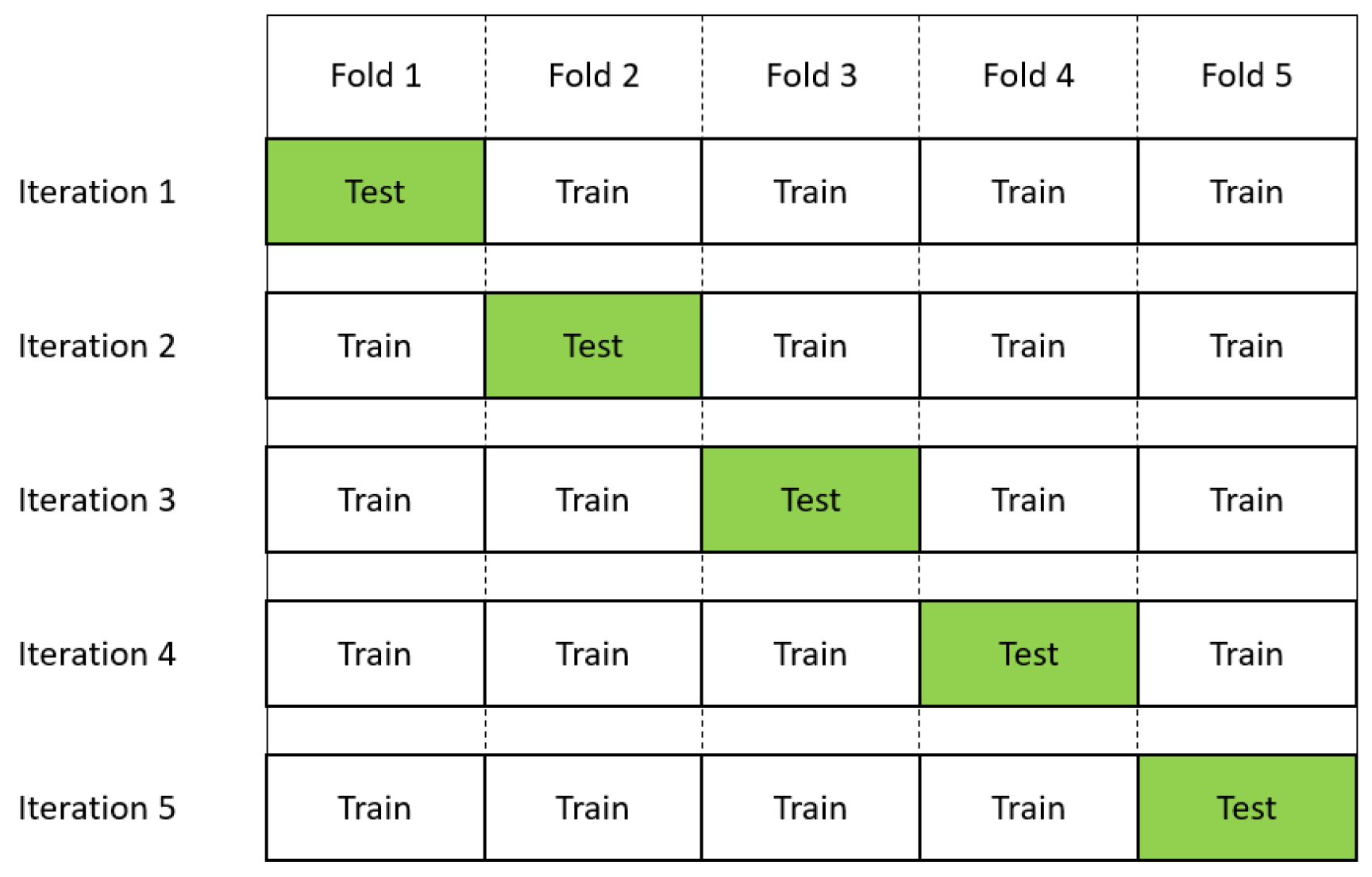
The dataset is divided into training and testing subsets, where the training data are used to calibrate the models and the testing data are used to evaluate predictive performance. Model validation is conducted using a K-fold cross-validation procedure, in which the dataset is randomly partitioned into K subsets. In each iteration, K–1 subsets are used for training and the remaining subset for testing. This process is repeated K times (See Figure 3), and error metrics are computed for each iteration; the final performance indicators are reported as the average across all folds.
In this study, a fivefold cross-validation was implemented, such that in each step, 80% of the data were used for training and the remaining 20% were used for testing.
The performance of the cluster classification is evaluated using accuracy (Equation (1)), while the predictive performance of the models is assessed using the coefficient of determination (R2 (Equation (2)) and the mean absolute percentage error (MAPE (Equation (3)).
A c c u r a c y = N u m b e r   o f   C o r r e c t   P r e d i c t i o n s T o t a l   n u m b e r   o f   P r e d i c t i o n s
R 2 = 1 i = 1 n Y i Y ^ i 2 i = 1 N Y i Y ¯ 2
M A P E % = i = 1 n Y i Y ^ i Y i n
Let Yi denote the predicted value, Y ^ i the observed value, Ȳ the mean of observed values, and n the number of observations. Under these definitions, both accuracy and R2 take values in the range [0,1], with 1 representing perfect prediction, whereas MAPE ranges between 0% and 100%, with lower values indicating better performance and 0% representing the optimal case.
Performance analysis in many reference works such as ASHRAE [57] also considers metrics such as CV (RMSE) and NMBE. Although these would have been interesting in some of the models (i.e., Q–T and MVLR), their definition in [57] required the explicit definition of the number of parameters in the model. To avoid this issue, these metrics were not used.
In addition, to predictive accuracy, execution time was measured for all models and compared to that of the Q–T algorithm to quantify the computational efficiency gained through the proposed DT identification and attribution process. Computational time is defined as the elapsed time required to train and test each multi-step model. All experiments were conducted on a personal laptop (the processor is an Intel(R) Core (TM) i5-10210U CPU @ 1.60GHz 2.11 GHz with 8 GB RAM); therefore, execution times should be interpreted as relative measures, since absolute runtimes would decrease substantially if executed on a dedicated server.

4. Results & Discussion

This section presents the results obtained for the intermediate steps of the proposed methodology, as well as the final HL prediction outcomes, evaluated using the error metrics defined in Section 3.5. All reported values correspond to the average results across the fivefold cross-validation procedure described previously.

4.1. DT Identification and Attribution

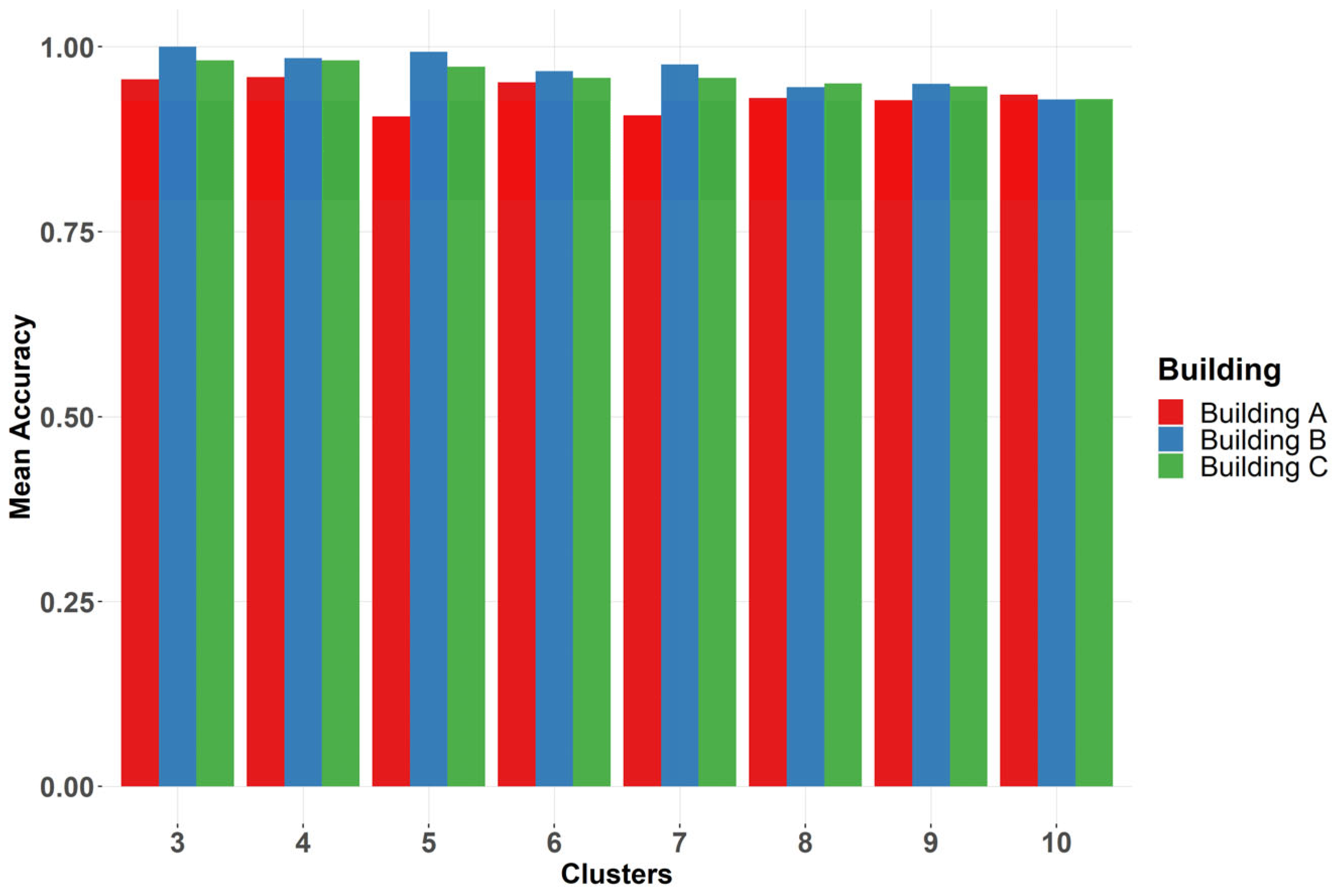
The classification algorithm achieved accuracies ranging from 0.8 to 1.0, with typical values around 0.9. This result was consistent across all buildings and for different numbers of clusters, although minor variations were observed. The classification process yielded slightly higher accuracies for Buildings B and C, whereas a small reduction in performance was observed as the number of clusters increased. Figure 4 illustrates the mean prediction accuracy (after the K-fold cross-validation process) of the classification model as a function of the number of clusters for the three buildings.

4.2. Heat Load Prediction

This section presents the results of the hourly HL prediction using the models defined in Section 3.4, both with and without DT attribution processes. The analysis is organized into two parts. First, linear models are compared against the Q–T model (Section 4.2.1). Then, the performance of machine learning (ML) models is evaluated (Section 4.2.2).

4.2.1. Performance of Linear Models

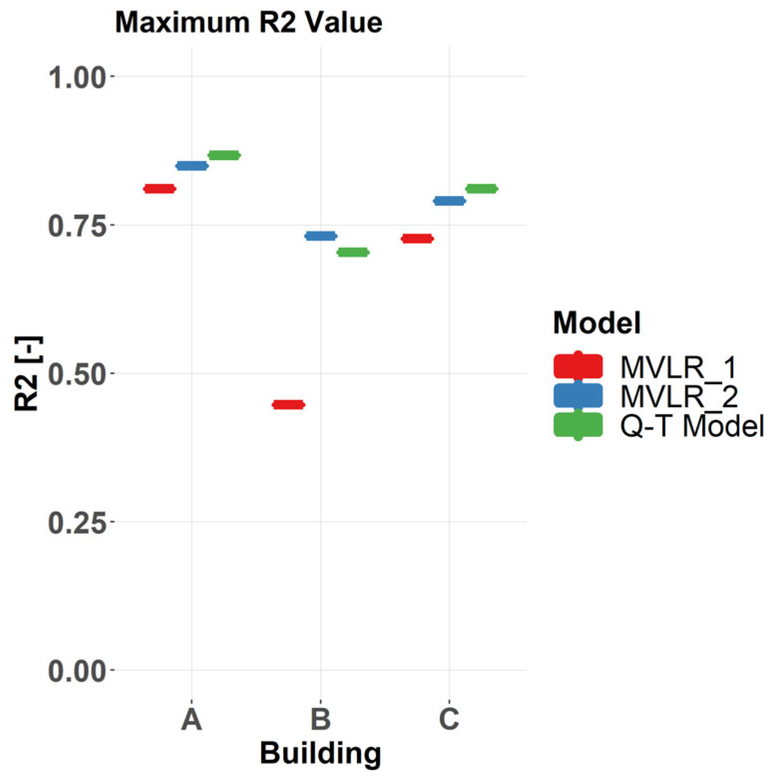
Figure 5 shows the R2 values obtained with the Q–T, MVLR_1, and MVLR_2 algorithms for the three buildings. The reported values correspond to models using the optimal number of clusters for DT attribution. Overall, the MVLR algorithms yield slightly lower R2 values than the baseline Q–T model. An exception is observed for Building B, where MVLR_2 slightly outperforms the Q–T model. Incorporating Day Type (DT) information substantially improves the performance of MVLR models, particularly for Building B, where MVLR_1 exhibits limited predictive capability (R2 < 0.5) due to high HL variability. Optimal results for MVLR_2 are achieved with three clusters for Building B and six clusters for Buildings A and C.
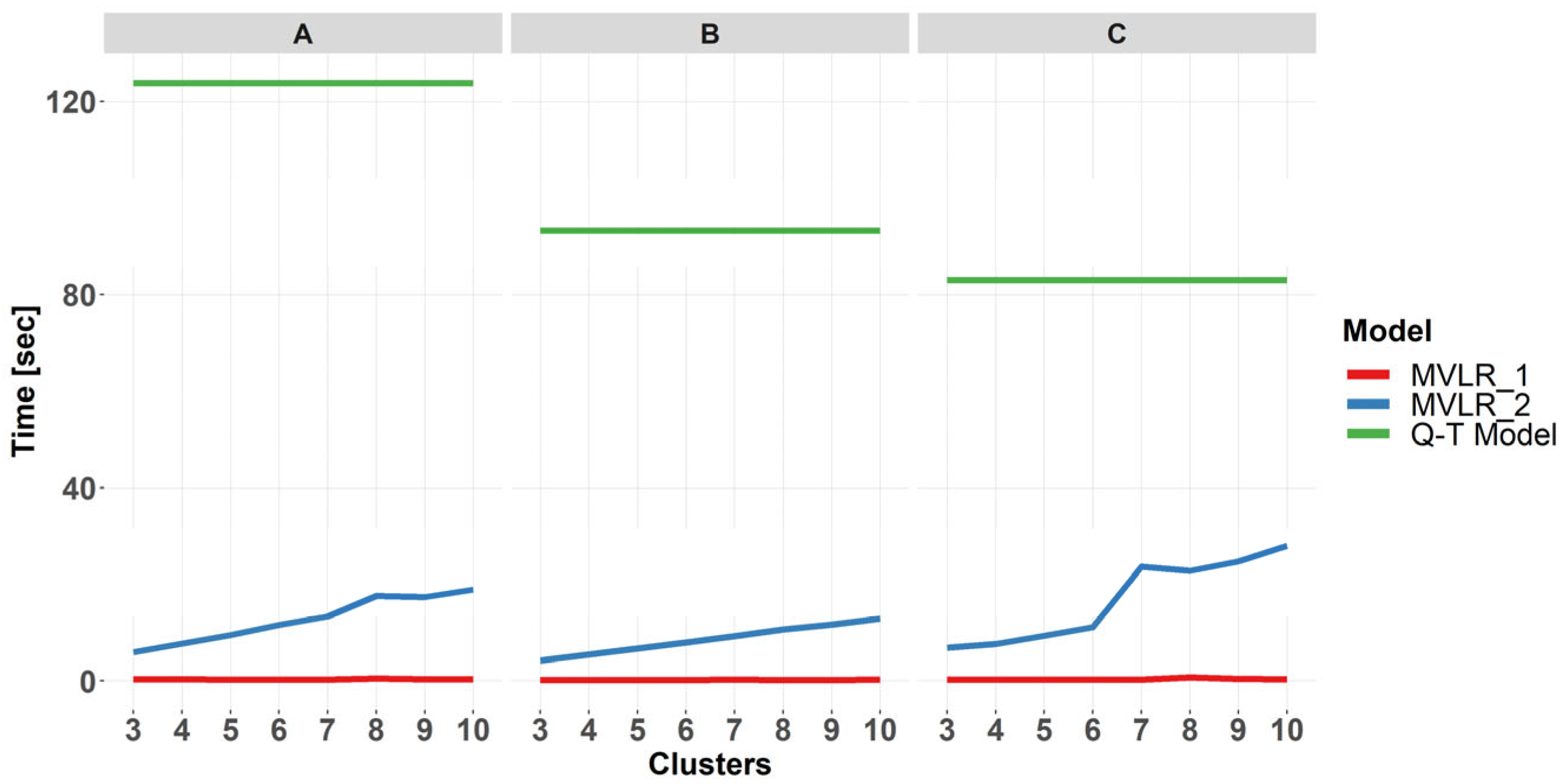
Figure 6 presents the computational times for Q–T, MVLR_1, and MVLR_2. All three buildings exhibit similar trends. The Q–T algorithm requires the highest computational time, ranging from 1 to 2 min, whereas MVLR_1 incurs negligible computation time. Since these algorithms do not incorporate DT attribution, their computational times are insensitive to the number of clusters. In contrast, MVLR_2 exhibits intermediate computation times, increasing with the number of DTs. For the number of DTs yielding optimal prediction, MVLR_2 reduces computational time by approximately 85% relative to the Q–T algorithm, ranging between 10 s and roughly one-third of the Q–T runtime.
These results indicate that MVLR_2 maintains predictive accuracy comparable to the Q–T algorithm while significantly reducing computational cost. A summary of these findings is provided in Table 3.
Based on these results, Section 4.2.2 evaluates the performance of ML models in comparison to MVLR models.

4.2.2. Performance of ML Models

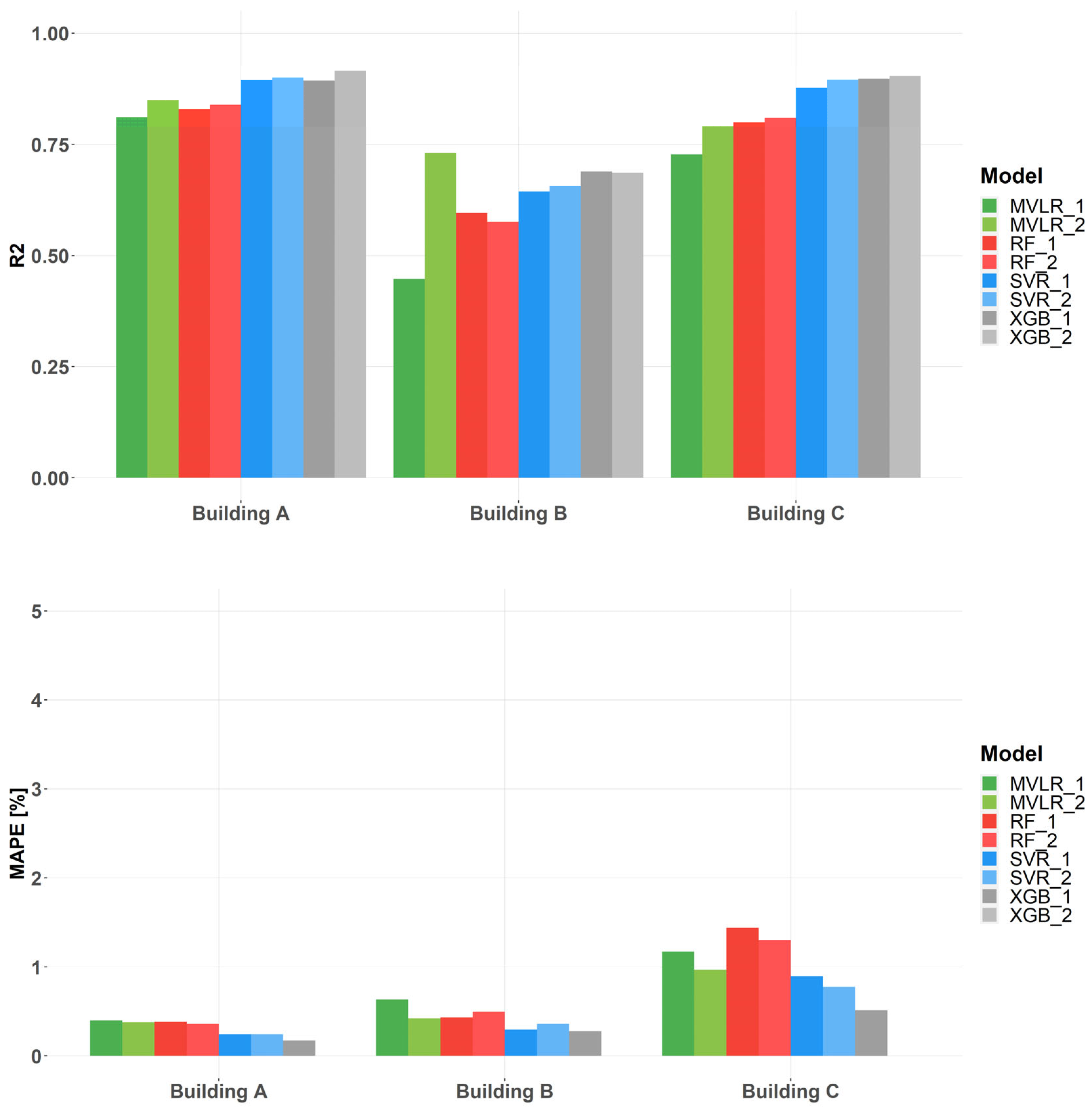
Figure 7 presents the R2 and MAPE values for the RF, SVR, and XGB models in comparison to the MVLR results. Overall, XGB achieves the highest performance in terms of both R2 and MAPE, consistent with findings reported in the literature. Model performance generally follows the following order: XGB > SVR > RF > MVLR. In most cases, incorporating Day Type (DT) attribution enhances predictive accuracy; however, this effect is not observed for Building B.
For Building B, although MAPE values remain very low (~<0.5%), R2 values are only in the moderate range (0.5–0.7) across all models. In addition, RF models underperform relative to MVLR for Building C.
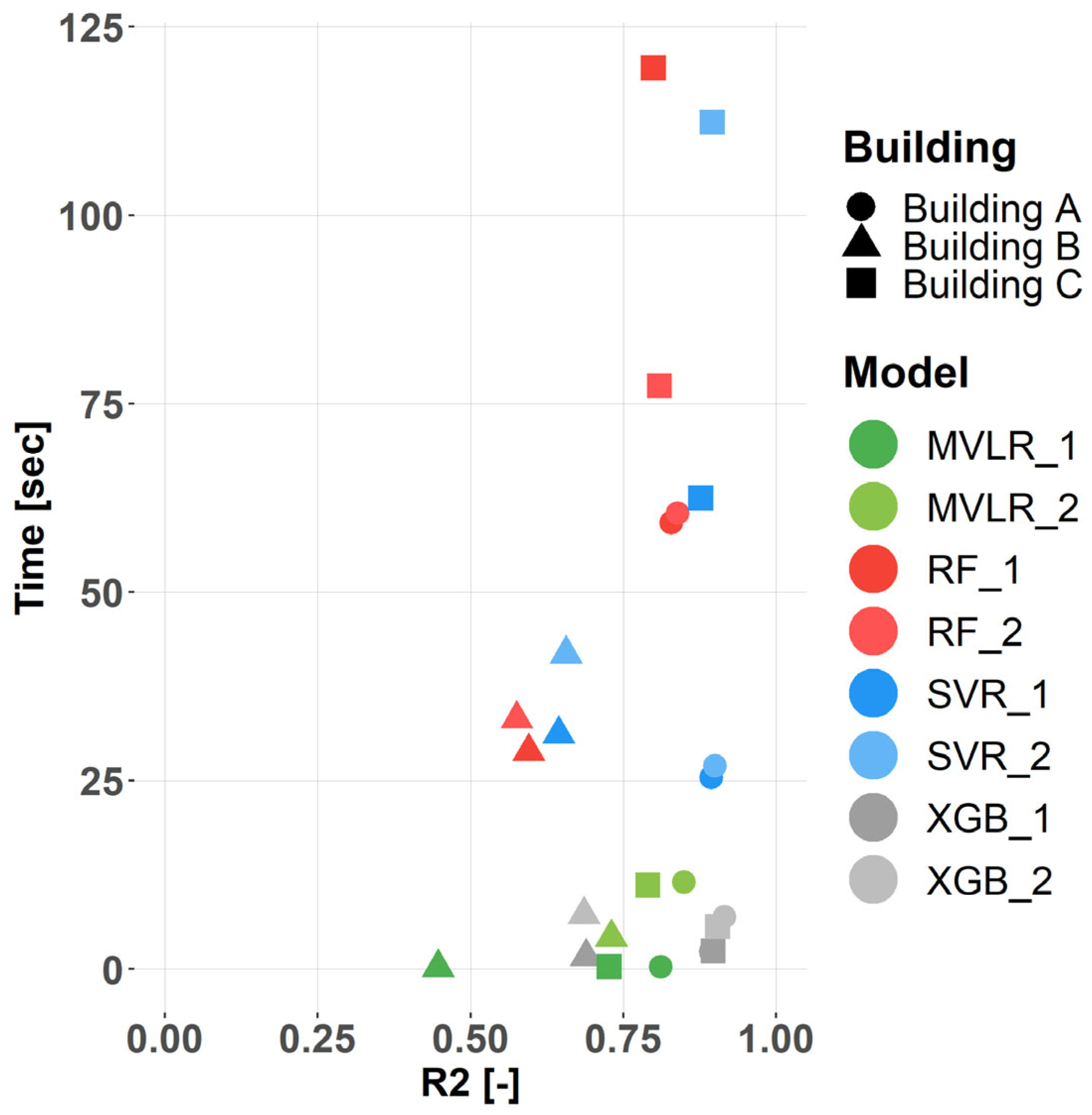
Regarding computational efficiency, XGB and MVLR models consistently require less than 20 s, whereas RF and SVR exhibit higher and more variable runtimes, ranging from 25 to 125 s. The impact of DT attribution on computation time varies across models and buildings. For instance, in Building D, DT attribution substantially reduces the computation time for RF models, whereas SVR models experience an increase in runtime.
Figure 8 illustrates the trade-off between computation time and predictive accuracy (R2) for the different models.

5. Conclusions

This paper presents a multi-step methodology for predicting Heat Loads (HLs) in buildings, integrating unsupervised and supervised learning techniques:
  • Unsupervised learning is employed to cluster HL profiles into a set of Day Types (DTs). Unlike conventional approaches based on the day of the week, this method assigns DTs based on actual performance, allowing for the better representation of variations such as bank holidays and seasonal shifts in peak loads.
  • Supervised learning is applied to attribute DTs to each day using only exogenous information (e.g., calendar and weather data).
  • Supervised learning is then used to predict hourly HLs for each building.
The methodology is designed to produce accurate yet compact models, facilitating scalability to large numbers of buildings. Model performance was evaluated not only in terms of predictive accuracy but also computational efficiency, using HL data from three real buildings with distinct load profiles. The Q–T algorithm, previously tested on the same dataset, was used as a baseline for both accuracy and computation time. Various supervised learning models were analyzed, and the benefits of incorporating DT attribution were systematically assessed.
Key findings from the study are summarized as follows:
  • Prediction accuracy: All models achieve good predictive performance, with MAPE values below 1.5% across all cases. R2 values range from moderate (~0.5–0.7 for Building B) to good (~0.7–0.85).
  • The most accurate model varies for each case: In building A, RF, SVR, and XGB perform comparably and substantially outperform MVLR. For Building C, XGB achieves the highest accuracy, with SVR and MVLR_2 outperforming RF. And for Building B, all models except MVLR_1 achieve similar MAPE values; MVLR_1 shows the highest (but still relatively low) R2.
  • Computational efficiency: All models exhibit substantially lower computation times than the Q–T algorithm. Even with the additional DT attribution step, the total computation time remains lower than for Q–T, and the time required for DT classification can be offset by faster HL models.
  • Impact of DT attribution on model accuracy: DT attribution improves predictive accuracy in most cases, with gains ranging from 2% to 50%, without significant computational overhead. This is particularly noticeable in Buildings B and C when assessing MVLR and RF (only in Building C).
  • Impact of DT attribution on model size: DT-based segmentation allows for smaller models, reducing the number of independent hourly models required. For Buildings B and C, three DTs are sufficient, halving a model size relative to Q–T. Building A required six DTs.
  • Impact of DT attribution on computational efficiency: Passing DT information to models reduces the need to internally infer occupant behavior, contributing to reduced computation times—up to 90% faster for MVLR compared to Q–T.
  • ML model comparison: XGB consistently achieves the highest predictive performance across all three buildings. MVLR and XGB models maintain computation times below 20 s for all buildings, whereas RF and SVR show higher and more variable runtimes (25–60 s, up to 120 s for Building C).
Overall, the multi-step methodology demonstrates strong potential for reducing computation time in HL prediction while maintaining high accuracy, particularly when model compactness and efficiency are key considerations.
A key takeover is that building heat loads are heavily related to social behaviors and that their identification (i.e., DT clustering and attribution) is key in improving load forecasting capacity, as well as reducing computation time.
Although the detailed interpretability of some of the physical models (i.e., MVLR) is unclear after DT attribution and the development of specific hourly models, this seems to be an approach resulting in fast and accurate models.
However, the study does not definitively identify the best-performing model for each building. Although it seems that XGB models may be a viable option in most cases, this shall be further investigated.
This work focuses on medium- and large-sized buildings in a cold climate with three specific usage types. It is anticipated that different building types and sizes under varied climate conditions will yield different results, warranting further investigation. Particularly, the following research questions remain for future research:
-
In our approach, we have been able to identify different usage patterns (clusters), but there is still a clearly observable physical significance in energy performance, associated with a cold climate. To what extent will this be so in milder climates? Is this approach also possible for buildings with heating and cooling loads?
-
The record in our dataset corresponds to actual observations in heat loads and meteorological data. In forecasting applications, it is likely that some deviation between the predicted and actual climate will result in variations in the actual load. Its impact on the accuracy of our method is yet to be determined.
-
The proposed methods develop a pattern identification and attribution process, based on the performance for a single year (2019). Can these patterns and their distribution throughout the year be stable and predictable with the CART approach? This is a relevant question calling for longitudinal research, even without considering the sharp behavioral changes in events such as those arising from the COVID crisis in 2020.
-
We define DT based on calendar information, where bank holidays are encoded. But our approach did not explicitly consider behavioral holidays (i.e., periods between a bank holiday and a weekend). Were these to be considered, it would potentially be a source for accuracy improvement in the CART process.
-
What is the trade-off when defining the optimal number of clusters? We believe that clustering processes are only reasonable to use if they allow for a reduction in model size and/or sorting out specific seasonal performance (i.e., spring break), but any cluster should still be useful in describing a relatively large number of days. Considering this, the number of clusters should be somewhere between 3 and 10–15, but this requires further research.

Author Contributions

Conceptualization, M.L.; Methodology, M.L., G.D., and K.M.-E.; Software, M.L.; Validation, M.L., R.G.-M., and B.A.; Formal analysis, M.L., R.G.-M., G.D., K.M.-E., and B.A.; Writing—original draft, M.L. and R.G.-M.; Writing—review and editing, G.D., K.M.-E., and B.A.; Visualization, M.L.; Supervision, G.D. and K.M.-E. All authors have read and agreed to the published version of the manuscript.

Funding

This research received no external funding.

Data Availability Statement

Data available on request due to restrictions, e.g., privacy or ethical restrictions. The data presented in this study are available on request from the corresponding author. The data are not publicly available due to commercial reasons and data privacy issues.

Acknowledgments

The authors would like to thank GREN Eesti for providing data from the substations for academic purposes.

Conflicts of Interest

The authors declare no conflict of interest.

Nomenclature

Acronyms
ARXAuto-Regressive models with eXogenous
ASHRAEAmerican Society of Heating, Refrigerating, and Air-Conditioning Engineers
DBSCANDensity-Based Spatial Clustering of Applications with Noise
DTDay type
DHNDistrict-Heating Network
DHWDomestic Hot Water
ECEuropean Commission
ESEnergy Signature
EUEuropean Union
HDDHeating Degree Day
HLHeat Load
HVACHeating Ventilation and Air Conditioning
kNNk-Nearest Neighborhood
MAPEMean Absolute Percentage Error
MLMachine Learning
MVLRMulti Variate Linear Regression
NNNeural Network
PRISMPRInceton Scorekeeping Method
Q–TSo-called Q–T algorithm in [8]
RESRenewable Energy Sources
RFRandom Forest
SARIMASeasonal Autoregressive Integrated Moving Average
SHSpace Heating
SVRSupport Vector Regressor
XGBExtreme Gradient Boosting
Symbols
GTSolar Radiation [W/m2]
MAPEMean Absolute Percentage Error [%]
nNumber of observations [-]
R2Coefficient of Determination [-]
TOUTOutdoor temperature [°C]
YPredicted Heat Load [kWh] or heat load vector
Y ¯ Known Heat Load [kWh] or heat load vector
μ Load Mean Value [kWh]

References

  1. International Energy Agency. Global Energy & CO2 Status Report 2019; IEA: Paris, France, 2019. [Google Scholar]
  2. Pérez-Lombard, L.; Ortiz, J.; Pout, C. A review on buildings energy consumption information. Energy Build. 2008, 40, 394–398. [Google Scholar] [CrossRef]
  3. Somu, N.; Ramam, G.; Ramamritham, K. A hybrid model for building energy consumption forecasting using long short term memory networks. Appl. Energy 2020, 261, 114131. [Google Scholar] [CrossRef]
  4. Jang, J.; Han, J.; Leigh, S.B. Prediction of heating energy consumption with operation pattern variables for non-residential buildings using LSTM networks. Energy Build. 2022, 255, 111647. [Google Scholar] [CrossRef]
  5. European Commission. Directive 2012/27/EU of the European Parliament and of the Council of 25 October 2012 on Energy Efficiency, Amending Directives 2009/125/EC and 2010/30/EU and Repealing Directives 2004/8/EC and 2006/32/EC Text with EEA Relevance OJ L 315; European Commission: Brussels, Belgium, 2012. [Google Scholar]
  6. European Commission. Directive (EU) 2018/844 of the European Parliament and of the Council of 30 May 2018 Amending Directive 2010/31/EU on the Energy Performance of Buildings and Directive 2012/27/EU on Energy Efficiency; European Commission: Brussels, Belgium, 2018. [Google Scholar]
  7. Liu, D.; Wang, W.; Liu, J. Sensitivity Analysis of Meteorological Parameters on Building Energy Consumption. Energy Procedia 2017, 132, 634–639. [Google Scholar] [CrossRef]
  8. Lumbreras, M.; Garay-Martinez, R.; Arregi, B.; Martin-Escudero, K.; Diarce, G.; Raud, M.; Hagu, I. Data driven model for heat load prediction in buildings connected to District Heating by using smart heat meters. Energy 2022, 239, 122318. [Google Scholar] [CrossRef]
  9. Buffa, S.; Cozzini, M.; D’Antoni, M.; Baratieri, M.; Fedrizzi, R. 5th generation district heating and cooling systems: A review of existing cases in Europe. Renew. Sustain. Energy Rev. 2019, 104, 504–522. [Google Scholar] [CrossRef]
  10. Frederiksen, S.; Werner, S. District Heating and Cooling; Studentlitteratur: Lund, Sweden, 2013; ISBN 9789144085302. [Google Scholar]
  11. Garay-Martinez, R.; Garrido-Marijuan, A. (Eds.) Handbook of Low Temperature District Heating; Green Energy and Technology; Springer: Cham, Swizerland, 2022; ISBN 978-3-031-10409-1. [Google Scholar] [CrossRef]
  12. Lumbreras, M.; Garay, R.; Marijuan, A.G. Energy meters in District-Heating Substations for Heat Consumption Characterization and Prediction Using Machine-Learning Techniques. IOP Conf. Ser. Earth Environ. Sci. 2020, 588, 032007. [Google Scholar] [CrossRef]
  13. Eguiarte, O.; Garrido-Marijuan, A.; Garay-Martinez, R.; Raud, M.; Hagu, I. Data-driven assessment for the supervision of District Heating Networks. Energy Rep. 2022, 8 (Suppl. 16), 34–40. [Google Scholar] [CrossRef]
  14. Sakkas, N.P.; Abang, R. Thermal load prediction of communal district heating systems by applying data-driven machine learning methods. Energy Rep. 2022, 8, 1883–1895. [Google Scholar] [CrossRef]
  15. do Carmo, C.M.R.; Christensen, T.H. Cluster analysis of residential heat load profiles and the role of technical and household characteristics. Energy Build. 2016, 125, 171–180. [Google Scholar] [CrossRef]
  16. Andersen, F.M.; Larsen Hv Boomsma, T.K. Long-term forecasting of hourly electricity load: Identification of consumption profiles and segmentation of customers. Energy Convers. Manag. 2013, 68, 244–252. [Google Scholar] [CrossRef]
  17. Hu, Y.; Li, J.; Hong, M.; Ren, J.; Man, Y. Industrial artificial intelligence based energy management system: Integrated framework for electricity load forecasting and fault prediction. Energy 2022, 244, 123195. [Google Scholar] [CrossRef]
  18. Jang, Y.; Byon, E.; Jahani, E.; Cetin, K. On the long-term density prediction of peak electricity load with demand side management in buildings. Energy Build. 2020, 228, 110450. [Google Scholar] [CrossRef]
  19. Chen, S.; Ren, Y.; Friedrich, D.; Yu, Z.; Yu, J. Prediction of office building electricity demand using artificial neural network by splitting the time horizon for different occupancy rates. Energy AI 2021, 5, 100093. [Google Scholar] [CrossRef]
  20. Dagdougui, H.; Bagheri, F.; Le, H.; Dessaint, L. Neural network model for short-term and very-short-term load forecasting in district buildings. Energy Build. 2019, 203, 109408. [Google Scholar] [CrossRef]
  21. Sandberg, A.; Wallin, F.; Li, H.; Azaza, M. An Analyze of Long-term Hourly District Heat Demand Forecasting of a Commercial Building Using Neural Networks. Energy Procedia 2017, 105, 3784–3790. [Google Scholar] [CrossRef]
  22. Cholewa, T.; Siuta-Olcha, A.; Smolarz, A.; Muryjas, P.; Wolszczak, P.; Guz, Ł.; Balaras, C.A. On the short term forecasting of heat power for heating of building. J. Clean. Prod. 2021, 307, 127232. [Google Scholar] [CrossRef]
  23. el Bouchefry, K.; de Souza, R.S. Learning in Big Data: Introduction to Machine Learning. In Knowledge Discovery in Big Data from Astronomy and Earth Observation: Astrogeoinformatics; Elsevier: Amsterdam, The Netherlands, 2020; pp. 225–249. [Google Scholar] [CrossRef]
  24. Belyadi, H.; Haghighat, A. Supervised learning. In Machine Learning Guide for Oil and Gas Using Python; Gulf Professional Publishing: Cambridge, MA, USA, 2021; pp. 169–295. [Google Scholar] [CrossRef]
  25. Celebi, M.E.; Aydin, K. Unsupervised Learning Algorithms; Springer International Publishing: Cham, Switzerland, 2016. [Google Scholar] [CrossRef]
  26. Hammarsten, S. A critical appraisal of energy-signature models. Appl. Energy 1987, 26, 97–110. [Google Scholar] [CrossRef]
  27. Fels, M.F. PRISM: An introduction. Energy Build. 1986, 9, 5–18. [Google Scholar] [CrossRef]
  28. Kissock, J.K.; Haberl, J.S.; Claridge, D.E. Change-Point Linear and Multiple-Linear Inverse Building Energy Analysis Models; Energy Systems Laboratory, Texas A&M University: College Station, TX, USA, 2002. [Google Scholar]
  29. Ferbar Tratar, L.; Strmčnik, E. The comparison of Holt–Winters method and Multiple regression method: A case study. Energy 2016, 109, 266–276. [Google Scholar] [CrossRef]
  30. Verbai, Z.; Lakatos, Á.; Kalmár, F. Prediction of energy demand for heating of residential buildings using variable degree day. Energy 2014, 76, 780–787. [Google Scholar] [CrossRef]
  31. Zhan, S.; Liu, Z.; Chong, A.; Yan, D. Building categorization revisited: A clustering-based approach to using smart meter data for building energy benchmarking. Appl. Energy 2020, 269, 114920. [Google Scholar] [CrossRef]
  32. Lumbreras, M.; Diarce, G.; Martin, K.; Garay-Martinez, R.; Arregi, B. Unsupervised recognition and prediction of daily patterns in heating loads in buildings. J. Build. Eng. 2023, 65, 105732. [Google Scholar] [CrossRef]
  33. Grosswindhager, S.; Voigt, A.; Kozek, M. Online Short-Term Forecast of System Heat Load in District Heating Networks. In Proceedings of the 31st International Symposium on Forecasting, Prague, Czech Republic, 27–29 June 2011. [Google Scholar]
  34. Eguizabal, M.; Garay-Martinez, R.; Flores-Abascal, I. Simplified model for the short-term forecasting of heat loads in buildings. Energy Rep. 2022, 8 (Suppl. 16), 79–85. [Google Scholar] [CrossRef]
  35. De Eulate, I.G.; Garay-Martinez, R.; Goikolea, B.A.; Eguiarte, O.; Macarulla, A.M. Simplified geometric processing of solar radiation for improved data-driven modelling of short-term energy & comfort performance in buildings. In Proceedings of the 2024 9th International Conference on Smart and Sustainable Technologies (SpliTech), Bol and Split, Croatia, 25–28 June 2024. [Google Scholar] [CrossRef]
  36. Bacher, P.; Madsen, H.; Nielsen, H.A.; Perers, B. Short-term heat load forecasting for single family houses. Energy Build. 2013, 65, 101–112. [Google Scholar] [CrossRef]
  37. Lei, L.; Chen, W.; Wu, B.; Chen, C.; Liu, W. A building energy consumption prediction model based on rough set theory and deep learning algorithms. Energy Build. 2021, 240, 110886. [Google Scholar] [CrossRef]
  38. Potočnik, P.; Škerl, P.; Govekar, E. Machine-learning-based multi-step heat demand forecasting in a district heating system. Energy Build. 2021, 233, 110673. [Google Scholar] [CrossRef]
  39. Dong, Z.; Liu, J.; Liu, B.; Li, K.; Li, X. Hourly energy consumption prediction of an office building based on ensemble learning and energy consumption pattern classification. Energy Build. 2021, 241, 110929. [Google Scholar] [CrossRef]
  40. MacQueen, J.B. Some methods for classification and analysis of multivariate observations. In Proceedings of the Fifth Berkeley Symposium on Mathematical Statistics and Probability, Berkeley, CA, USA, 21 June–18 July 1965 and 27 December 1965–7 January 1966; Volume 1, pp. 281–297. [Google Scholar]
  41. Park, J.Y.; Yang, X.; Miller, C.; Arjunan, P.; Nagy, Z. Apples or oranges? Identification of fundamental load shape profiles for benchmarking buildings using a large and diverse dataset. Appl. Energy 2019, 236, 1280–1295. [Google Scholar] [CrossRef]
  42. Wen, L.; Zhou, K.; Yang, S. A shape-based clustering method for pattern recognition of residential electricity consumption. J. Clean. Prod. 2019, 212, 475–488. [Google Scholar] [CrossRef]
  43. Gianniou, P.; Liu, X.; Heller, A.; Nielsen, P.S.; Rode, C. Clustering-based analysis for residential district heating data. Energy Convers. Manag. 2018, 165, 840–850. [Google Scholar] [CrossRef]
  44. R Core-Team. A Language and Environment for Statistical Computing; R Foundation for Statistical Computing: Vienna, Austria, 2013. [Google Scholar]
  45. University of Tartu, Institute of Physics, Laboratory of Environmental Physics. 2021. Available online: http://meteo.physic.ut.ee/?lang=en (accessed on 30 September 2022).
  46. Ester, M.; Kriegel, H.; Xu, X.; Miinchen, D. A Density-Based Algorithm for Discovering Clusters in Large Spatial Databases with Noise. In Proceedings of the 2nd ACM SIGKDD, Portland, OR, USA, 2–4 August 1996; pp. 226–231. [Google Scholar]
  47. Hashler, M.; Piekenbrock, M.; Arya, S.; Mount, D.R. Package ’dbscan’ 2020. 2021. Available online: https://cran.r-project.org/ (accessed on 30 September 2022).
  48. Walsh, A.; Cóstola, D.; Labaki, L.C. Performance-based climatic zoning method for building energy efficiency applications using cluster analysis. Energy 2022, 255, 124477. [Google Scholar] [CrossRef]
  49. Fix, E.; Hodges, J.L. Discriminatory Analysis. Nonparametric Discrimination: Consistency Properties. Int. Stat. Rev. 1989, 57, 238. [Google Scholar] [CrossRef]
  50. class: Functions for Classification 2022. Available online: https://cran.r-project.org/package=class (accessed on 30 September 2022).
  51. Cortes, C.; Vapnik, V. Support-vector networks. Mach. Learn. 1995, 20, 273–297. [Google Scholar] [CrossRef]
  52. Meyer, D.; Dimitriadou, E.; Weingessel, A.; Leisch, F. e1071: Misc Functions of the Department of Statistics, Probability Theory Group (Formerly: E1071), TU Wien 2022. Available online: https://cran.r-project.org/ (accessed on 30 September 2022).
  53. Breiman, L. Random forests. Mach. Learn. 2001, 45, 5–32. [Google Scholar] [CrossRef]
  54. Liaw, A.; Wiener, M. Classification and Regression by randomforest.r News, vol 2/3, 2002. Available online: https://journal.r-project.org/issues/2002-3/ (accessed on 6 October 2025).
  55. Chen, T.; Guestrin, C. XGBoost: A Scalable Tree Boosting System. In Proceedings of the 22nd ACM SIGKDD International Conference on Knowledge Discovery and Data Mining (KDD ’16), San Francisco, CA, USA, 13–17 August 2016; pp. 785–794. [Google Scholar] [CrossRef]
  56. Chen, T.; He, T.; Benesty, M. xgboost: Extreme Gradient Boosting. 2022. Available online: https://cran.r-project.org/ (accessed on 30 September 2022).
  57. ASHRAE. ASHRAE Guideline 14-2014, Measurement of Energy, Demand, and Water Savings; ASHRAE: Atlanta, GA, USA, 2014. [Google Scholar]
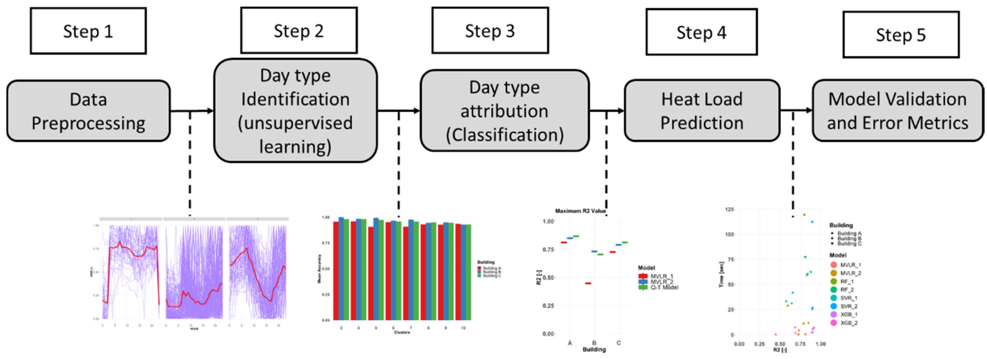
Figure 1. General framework of the paper (larger-sized figures of the specific process outcomes are available in Figures 4, 5, and 7 of this paper and Figure 4 of [32]).
Buildings 15 03604 g001
Figure 2. Hourly energy consumption vs. outdoor temperature for (a) Building A, (b) Building B, and (c) Building C.
Buildings 15 03604 g002
Figure 3. K-fold Cross validation methodology (K = 5).
Buildings 15 03604 g003
Figure 4. Mean Accuracy (K-fold) using the kNN algorithm for cluster prediction.
Buildings 15 03604 g004
Figure 5. Maximum R2 values for the three buildings using multi-variable linear regressions.
Buildings 15 03604 g005
Figure 6. Computational time required for the linear models in each building.
Buildings 15 03604 g006
Figure 7. Performance metrics for the different models. R2 (Above) and MAPE (Below).
Buildings 15 03604 g007
Figure 8. Computation Time vs. R2 for the three buildings.
Buildings 15 03604 g008
Table 1. Variables used for the kNN classification model to predict the cluster.
VariableUnitsType of Data
Daily Mean Temperature°CNumeric
Daily Total RadiationWh/m2Numeric
Holiday[-]Boolean
Day of the Week[-]Categorical
Month of the Year[-]Categorical
Day preceding a Holiday[-]Boolean
Table 2. Predictive Models and the predictors used in each model.
AlgorithmModelTOUTGTWeek
Day
MonthHour DayHolidayCluster
Q–TQ–TX XX
MVLRMVLR_1XX X
MVLR_2XX X X
SVRSVR_1XXXXXX
SVR_2XXXXXXX
RFRF_1XXXXXX
RF_2XXXXXXX
XGBXGB_1XXXXXX
XGB_2XXXXXXX
Table 3. Comparison between the results obtained with the Q–T algorithm vs. MVLR_2.
Q–T R2 [-]MVLR_2 Optimal Number of ClustersMVLR_2 R2 [%]Q–T Time [s]MVLR_2 Time [%]
Building A0.8676−1.98%123.81−90.79%
Building B0.7043+3.81%93.27−95.50%
Building C0.8113−2.53%82.97−86.60%
Disclaimer/Publisher’s Note: The statements, opinions and data contained in all publications are solely those of the individual author(s) and contributor(s) and not of MDPI and/or the editor(s). MDPI and/or the editor(s) disclaim responsibility for any injury to people or property resulting from any ideas, methods, instructions or products referred to in the content.