Article

A Box-Based Method for Regularizing the Prediction of Semantic Segmentation of Building Facades

by
Shuyu Liu
1,
Zhihui Wang
1,
Yuexia Hu
1,
Xiaoyu Zhao
1 and
Si Zhang
2,*
1
College of Architecture, Nanjing Tech University, Nanjing 211816, China
2
College of Art & Design, Nanjing Tech University, Nanjing 211816, China
*
Author to whom correspondence should be addressed.
Buildings 2025, 15(19), 3562; https://doi.org/10.3390/buildings15193562 (registering DOI)
Submission received: 10 July 2025 / Revised: 20 September 2025 / Accepted: 30 September 2025 / Published: 2 October 2025
(This article belongs to the Section Architectural Design, Urban Science, and Real Estate)

Abstract

Semantic segmentation of building facade images has enabled a lot of intelligent support for architectural research and practice in the last decade. However, the classifiers for semantic segmentation usually predict facade elements (e.g., windows) as graphics in irregular shapes. The non-smooth edges and hard-to-define shapes impede the further use of the predicted graphics. This study proposes a method to regularize the predicted graphics following the prior knowledge of composition principles of building facades. Specifically, we define four types of boxes for each predicted graphic, namely minimum circumscribed box (MCB), maximum inscribed box (MIB), candidate box (CB), and best overlapping box (BOB). Based on these boxes, a three-stage process, consisting of denoising, BOB finding, and BOB stacking, was established to regularize the predicted graphics of facade elements into basic rectilinear polygons. To compare the proposed and existing methods of graphic regularization, an experiment was conducted based on the predicted graphics of facade elements obtained from four pixel-wise annotated building facade datasets, Irregular Facades (IRFs), CMP Facade Database, ECP Paris, and ICG Graz50. The results demonstrate that the graphics regularized by our method align more closely with real facade elements in shape and edge. Moreover, our method avoids the prevalent issue of correctness degradation observed in existing methods. Compared with the predicted graphics, the average IoU and F1-score of our method-regularized graphics respectively increase by 0.001–0.017 and 0.000–0.012 across the datasets, while those of previous method-regularized graphics decrease by 0.002–0.021 and 0.002–0.015. The regularized graphics contribute to improving the precision and depth of semantic segmentation-based applications of building facades. They are also expected to be useful for the exploration of data mining on urban images in the future.

1. Introduction

In the big data era, massive architectural images have been captured and shared worldwide [1,2]. Among various image types, the images of building facades receive a lot of attention from architects [3]. By applying the latest semantic segmentation methods to these images, various facade elements (e.g., windows) can be automatically identified by the well-trained classifiers [4,5,6]. The identified facade elements are essential to the fields of 3-D reconstruction [7], building damage detection [8,9], energy evaluation [10,11], building and city information modeling [12,13], architectural knowledge discovery [14], etc.
However, there is still a problem that limits the effect and scope of the application of the identified elements. In the segmented facades, each element is predicted as a graphic that consists of pixels of the same class [15]. Since the predicted graphics are commonly irregular, the non-smooth edges and hard-to-define shapes severely weaken the ability of the graphics to convey information [16]. Compared to the ground truth, the area, position, and shape of the predicted graphics changed significantly, thus negatively affecting the completeness and correctness of the information of building facades, as shown in Figure 1. As prior studies [17,18] suggest, this problem is caused by complex factors that are difficult to avoid completely, such as image resolution, technical limitations, etc. To improve the quality of the identified elements, therefore, it is necessary to convert the predicted graphics back to regular shapes that conform to the composition characteristics of building facades.
This study proposes a box-based method that transforms the irregular predicted graphics of facade elements into basic rectilinear polygons with smooth edges, such as rectangular, L-, U-, and T-shapes. For each predicted graphic, we generate several candidate boxes (CB) by horizontal and vertical boundary sliding within its minimum circumscribed box (MCB) and maximum inscribed box (MIB), and define the CB with the highest Intersection over Union (IoU) with the graphic as its best overlapping box (BOB). Then, the BOBs are stacked sequentially onto the same layer according to their IoU from low to high. Graphics in this layer are regular and used to replace the original irregular ones.
To achieve this goal, we introduce two principles of the composition characteristics of building facades and rigorously define the four types of boxes mentioned above. A three-stage process of graphic regularization, consisting of denoising, BOB finding, and BOB stacking, is established based on the principles and boxes. An experiment was carried out to validate the effect of this method. The results demonstrate that the proposed method possesses two primary advantages compared to previous methods of graphic regularization: (1) the graphics regularized by our method exhibit closer alignment with real facade elements in terms of shape and edge; (2) the correctness of the regularized graphics shows no degradation compared to the predicted graphics. Ablation analysis confirms that BOB—the core tool of the proposed method—functions as intended.
For the task of graphic regularization, this study has the following contributions.
  • The proposed method regularizes the predicted graphics into basic rectilinear polygons that conform to the composition characteristics of building facades. The regularized graphics are useful for many image-based applications of building facades.
  • A simple yet effective mechanism of graphic regularization is provided, which can be applied to other similar tasks easily and flexibly.
  • This study demonstrates the importance of prior knowledge in regularization tasks, serving as a reference for related research.
The rest of this paper is organized as follows. Section 2 reviews previous methods and literature of graphic regularization. The principles, boxes, process, and complexity of the proposed method are introduced in Section 3. Section 4 reports the adopted data, procedure, and results of the experiment. Section 5 and Section 6 discuss the core idea, future applications and limitations of this study. The main contributions of this study are summarized in Section 7.

2. Related Work

The regularization of graphics is a long-term focused field, and many relevant methods have been proposed. In general, these methods can be categorized into several technical types, i.e., the polygon-, conversion-, and snake-based methods. We review these studies separately.

2.1. Polygon-Based Methods

Most studies in this field tried to reconstruct the graphic contour as an approximate polygon based on its basic geometric features, including vertices, area, and axes.

2.1.1. Vertex-Based Approaches

The Douglas–Peucker algorithm, also known as the DP algorithm, was one of the earliest successful algorithms developed for graphic regularization [19]. Its basic principle is using as few vertices as possible to reconstruct the graphic contour. For a continuous polyline, the DP algorithm recursively determines whether to remain or remove a vertex based on its distance from the straight line that connects the first and last vertices of the polyline. Based on the DP algorithm, Liu et al. proposed an adaptively improved algorithm (AIDP) that achieves automated polygonal approximation by integrating the criteria of vertical and radial distance restrictions [20]. As the DP algorithm does not consider the geometrical characteristics of graphics, most DP-based methods are sensitive to both the position of the starting point and the noise. To address this problem, Mousa et al. used the digital elevation model (DEM) to support graphic regularization. By combining the model- and data-driven approaches, their method regularizes the graphics more effectively [21].

2.1.2. Area-Based Approaches

Focusing on the area of graphics, a set of polygonal approximation schemes, namely the internal maximum area polygonal approximation (IMAPA), the external minimum area polygonal approximation (EMAPA), and the minimum area deviation polygonal approximation (MADPA), were proposed to generate approximation polygons for irregular contours [22]. The number of polygon sides can be adjusted flexibly to suit various application situations. Wang et al. selectively replaced part of the irregular graphic contour with the edge segmentation of its suitable circumscribed rectangle based on the Hausdorff distance. This method is effective to optimize the slightly missing building boundary caused by foreground, shadow, and other noise factors [23].

2.1.3. Axis-Based Approaches

Du et al. proposed an optimization-based linearization and global regularization to form accurate, topologically error-free, and lightweight polygons. Based on the dominant direction of each building, linear primitives decomposed from the initially segmented building contours are further simultaneously regularized by hierarchically employing parallelism, homogeneity, orthogonality, and collinearity criteria. In contrast to region- or even city-scale buildings, this method shows weaker performance in processing individual buildings [24]. Addressing the jagged and irregular problems of building contours, Pan et al. decomposed, corrected, simplified and connected building edges based on the extracted principal directions, thereby obtaining regular contours composed of straight lines and right angles [25].

2.2. Conversion-Based Methods

This type of method converts part of the initial contour information into other digital forms and regularizes the contours based on the converted data. Li et al. converted the two-dimensional initial building contour into a one-dimensional signal and equated the zig-zag shapes in the contour to the noise in the signal. By this way, the contour regularization task becomes a signal denoising task. Regular contours can be obtained based on the noise-free signals [26]. Chen et al. introduced the PolygonCNN that integrates their modified PointNet and a state-of-the-art convolutional neural network PSPNet. By encoding the vertices of the initial contour along with the pooled image features extracted from the PSPNet, the modified PointNet learns the shape priors, predicts the deformation of vertices, and generates the refined contour vertices [27,28].

2.3. Snake-Based Methods

The snake, or the active contour model, is a deformable continuous curve, whose shape is controlled by both internal and external forces. It gradually approaches the graphic contour under the constraints of internal forces (tension and bending) and the guidance of external forces (lines, edges, and terminations) [29]. Based on the parametric B-spline approximations of the curves, Menet et al. proposed B-snakes that allow for breakpoints and corners in the contour [30].
Focusing on the limitations caused by the internal forces, several variants of B-snakes were developed, including B-spline snakes [31], Locally Regularized B-Snakes [32], etc. In these studies, scholars replaced the internal forces with a series of new algorithms to simplify the process, improve the speed, and optimize the applicability of the convergence of prior snake versions.
On the contrary, some scholars paid more attention to the external forces. Xu and Prince devised the gradient vector flow (GVF) to compute the external forces. This change enabled the snake to be initialized flexibly, and its sensitivity to contour concavities was also enhanced [33]. Soon after, the GVF was generalized as GGVF to balance the smoothness and precision of the GVF field, thereby improving the snake convergence into long, thin boundary indentations [34]. Moreover, Chang et al. used the Minimum Bounding Rectangle (MBR) to support the GGVF, so that both the regularity and accuracy of complex building contours can be improved [35].

2.4. Summary

The abovementioned studies explored the methods of graphic regularization from multiple perspectives and significantly improved the effect and robustness of regularization. Since most of these methods were devised for building footprints, they cannot regularize the predicted graphics of building facade elements with the expected performance due to three key limitations.
First, the methods mentioned above place much more emphasis on the smoothness of the graphic contour rather than orthogonality. This preference is appropriate for building footprints in which many adjacent edges intersect at an oblique angle. On the contrary, most edges of building facade elements are horizontal or vertical. The graphics regularized by these methods cannot fully reflect the composition characteristics of building facades.
Second, the existing methods simplify the graphic contour without necessarily converting it to basic geometric shapes, such as rectangular, L-, U-, and T-shapes, because the shapes of building footprints are complex and varied. Considering that shape is a critical feature of facade elements, the graphics of only simple but not basic shapes make a limited contribution to the image-based analysis of building facades.
Third, as most building footprints are detached, many existing methods consider the common edge between different contours to be an error and seek to eliminate it. However, the facade elements are often adjacent or partly overlapped. As a result, indeed there are many common edges in building facades. These edges must not be ignored, and the corresponding regularization strategy is required.

3. Methodology

In this section, we introduce two principles of facade composition first in Section 3.1. Following these principles, four types of axis-aligned rectangular boxes are defined as the tools of regularization in Section 3.2. Based on these boxes, the process of graphic regularization is established in Section 3.3. Section 3.4 analyzes its time complexity.

3.1. Principles

To understand how our method works, two principles of the geometric characteristics of facade elements must be introduced in advance.

3.1.1. Principle 1: A Complex Shape Can Be Regarded as the Uncovered Part of a Partially Covered Rectangle

Rectangles are the most used shape in building facades. As shown in Figure 2, the horizontal and vertical divisions of the facade create lots of rectangular regions. Since the shape of the ground truth is known in advance, it becomes easy to regularize the predicted graphic of most facade elements.
Although most facade elements are rectangular, there are some elements in more complex shapes, such as L-, U-, and T-shapes. These non-rectangular elements increase the uncertainty of regularization. However, if we deconstruct the facade elements in non-rectangular shapes from the perspective of multi-layered composition, they can also be regarded as the result of a set of rectangular elements that overlap with each other. By partially covering a rectangle with other rectangle(s), the non-rectangular shapes can be obtained from the uncovered part of the former. Figure 3 shows several examples of how the elements in non-rectangular shapes are produced based on the overlapping rectangles.
In summary, most of the elements in building facades can be represented by one or more rectangles. This prior principle greatly reduces the difficulty of regularizing the predicted graphics of building facade elements.

3.1.2. Principle 2: The Higher the Complexity of a Graphic, the Lower Its Highest Achievable IoU with a Rectangle

According to principle 1, it is natural to regularize the predicted graphics of facade elements with rectangular boxes. For any graphic, there exists a rectangle that achieves the highest IoU with it. This highest achievable IoU varies depending on the shape of the graphic. As illustrated in Figure 4, the more (or less) similar a graphic is to a rectangle, the closer the highest achievable IoU is to 1 (or 0).
As stated in principle 1, a non-rectangular facade element can be regarded as the uncovered part of a rectangle that is partially covered by other rectangular elements. This mechanism can also interpret the relationship between a predicted graphic’s shape and its highest achievable IoU with rectangles: the more (or less) a facade element is covered, the closer its highest achievable IoU with rectangles is to 0 (or 1). This principle is important for determining the order in which graphics are regularized.

3.2. Definitions

In this section, four types of axis-aligned rectangular boxes are defined, namely minimum circumscribed box (MCB), maximum inscribed box (MIB), candidate box (CB), and best overlapping box (BOB). Specifically, each graphic has an MCB and an MIB. Between the MCB and MIB, there are several CBs of it. The CB achieves the highest IoU with this graphic is considered its BOB. The following are mathematical definitions of these boxes.
As shown in Figure 5a, for a segmented facade image I with a width of W pixels and a height of H pixels, a two-dimensional Cartesian coordinate system is built. In this coordinate system, the coordinates of the left-bottom pixel of image I are set to (1,1), while the coordinates of the right-top pixel are naturally (W, H). Let G be a predicted graphic within image I whose leftmost, bottommost, rightmost, and topmost pixel coordinates are L, B, R, and T, respectively, and let S be the set of all pixels contained within graphic G. As pixel-based variables, W, H, L, B, R, and T satisfy the following conditions:
W , H , L , B , R , T N
1 L R W
1 B T H
where N represents the set of positive integers.
Based on the coordinate system, the minimum circumscribed box (MCB), maximum inscribed box (MIB), candidate box (CB), and best overlapping box (BOB) of the graphic G is defined as follows. In these definitions, any box—an axis-aligned rectangle—is represented as a quadruple, whose four elements denote the pixel coordinates of the box’s left, bottom, right, and top boundaries, respectively, as shown in Figure 5b–e.
Definition 1.
Minimum circumscribed box (MCB)
The minimum circumscribed box of the graphic G is defined as an axis-aligned rectangle (LMCB, BMCB, RMCB, TMCB), where LMCB, BMCB, RMCB, and TMCB are equal to L, B, R, and T, respectively.
Definition 2.
Maximum inscribed box (MIB)
The maximum inscribed box of the graphic G is defined as an axis-aligned rectangle (LMIB, BMIB, RMIB, TMIB) as:
f l , b , r , t = r l × t b   s u b j e c t   t o   x l , r , y b , t , x , y S
L M I B , B M I B , R M I B , T M I B = argmax l , b , r , t   f l , b , r , t
In Equation (4), f(l, b, r, t) calculates the area of the box whose left, bottom, right, and top boundary coordinates are l, b, r, and t respectively, while the constraint ensures that all pixels constituting the box belong to the predicted graphic G. Equation (5) uses the quadruple that leads to the largest area to define the maximum inscribed box.
Definition 3.
Candidate box (CB)
A candidate box of the graphic G is any axis-aligned rectangle whose coordinates along one axis align with the MCB, while the coordinates along the other axis lie between the MCB and the MIB. Specifically, the candidate boxes are generated through two strategies: horizontal sliding and vertical sliding. The horizontal sliding strategy fixes the bottom and top coordinates of the candidate box to be the same as those of the MCB. By sliding pixel by pixel between the left coordinates of the MCB and the MIB, and between the right coordinates of the MCB and the MIB, a set of left coordinates and a set of right coordinates are obtained respectively. Each two cross-set coordinates are regarded as the left and right coordinates of a candidate box. Similarly, the vertical sliding strategy generates candidate boxes by fixing the left and right coordinates while sliding the bottom and top coordinates. Formally, the set C of all candidate boxes is defined as:
C H = L C B , B C B = B M C B , R C B , T C B = T M C B N 4 L M C B L C B L M I B R M I B R C B R M C B
C V = L C B = L M C B , B C B , R C B = R M C B , T C B N 4 B M C B B C B B M I B T M I B T C B T M C B
C = C H C V
where CH and CV represent the sets of candidate boxes generated through the horizontal and vertical sliding strategies, respectively; N4 represents the set of all integer quadruples. Each element in the set C corresponds to a candidate box (LCB, BCB, RCB, TCB).
It is evident that the above strategies do not traverse all axis-aligned rectangles whose spatial extent is constrained to lie between the MCB and the MIB, because it only slides the coordinates along one axis at a time. Theoretically, boxes that match better with graphic G might be generated if we slide the coordinates along both two axes simultaneously. However, this would inevitably lead to a substantial increase in computational cost. Considering that the predicted graphics rarely incur significant errors in all four directions, our strategies can balance both the quality and efficiency of candidate box generation, thus ensuring its feasibility for real-world tasks.
Definition 4.
Best overlapping box (BOB)
The best overlapping box (BOB) is defined as the candidate box that achieves the highest Intersection over Union (IoU) with the graphic G. Formally, the BOB (LBOB, BBOB, RBOB, TBOB) is defined as:
P = x , y N 2 L C B x R C B B C B y T C B   s u b j e c t   t o   L C B , B C B , R C B , T C B C
g L C B , B C B , R C B , T C B = P S P S
L B O B , B B O B , R B O B , T B O B = argmax L CB , B CB , R CB , T CB g L C B , B C B , R C B , T C B
where P denotes the set of all pixels contained within a candidate box. The set N2 represents the domain of all discrete, two-dimensional coordinates, where each element (x, y) ∈ N2 denotes a single pixel location in the image. g(LCB, BCB, RCB, TCB) calculates the IoU between a candidate box and the predicted graphic G. Equation (11) used the quadruple of the candidate box that leads to the highest IoU to define the best overlapping box.

3.3. Process

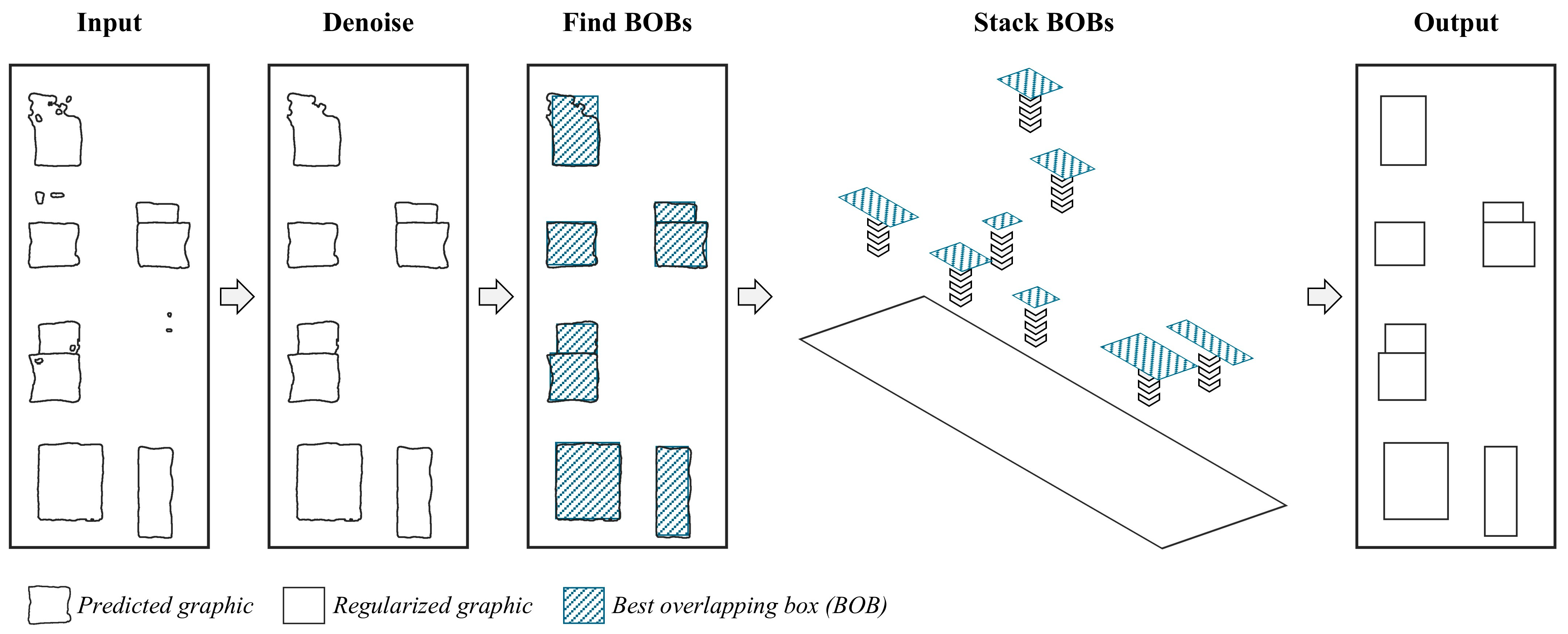
Based on the boxes, a process is established to regularize the predicted graphics of building facade elements. This process consists of three stages, i.e., denoising, BOB finding, and BOB stacking. In the first stage, noise in the segmented facade is excluded. After that, the best overlapping box of each predicted graphic is found in stage 2 and stacked onto the same layer in order in stage 3. Figure 6 visually illustrates this process while Algorithm 1 describes it in detail.
Algorithm 1. The box-based graphic regularization for segmented facades.
Input: A set of segmented facades with predicted graphics of facade elements
Output: A set of Segmented facades with regularized graphics of facade elements
1:for i in [1, m] (m = the number of input facade images)
2:        Regularize the predicted graphics in the i-th image
3:        # Stage 1: Denoising #
4:        Count the number of pixels of each graphic of facade elements
5:        Remove the graphics whose pixel count is below the threshold
6:        Fill the holes inside the graphics of facade elements
7:        # Stage 2: BOB finding #
8:        for j in [1, n] (n = the number of graphics in the denoised image)
9:                Locate the MCB (LMCB, BMCB, RMCB, TMCB) of the j-th graphic
10:                Locate the MIB (LMIB, BMIB, RMIB, TMIB) of the j-th graphic
11:                # Horizontal sliding #
12:                for LCB in [LMCB, LMIB]
13:                        for RCB in [RMIB, RMCB]
14:                                Generate a CB [LCB, BCB = BMCB, RCB, TCB = TMCB]
15:                                Compute the IoU between the CB and the j-th graphic
16:                # Vertical sliding #
17:                for BCB in [BMCB, BMIB]
18:                        for TCB in [TMIB, TMCB]
19:                                Generate a CB [LCB = LMCB, BCB, RCB = RMCB, TCB]
20:                                Compute the IoU between the CB and the j-th graphic
21:                Select the CB with the highest IoU as the BOB of the j-th graphic
22:        until the BOBs of all graphics are found
23:        # Stege 3: BOB stacking #
24:        Sort the BOBs in ascending order of their IoU
25:        Stack the BOBs onto the same layer according to this order
26:        Replace the pixels in the i-th image with those from this layer
27:        # Return #
28:        return the i-th facade image with regularized graphics
29:until all input facade images are regularized

3.3.1. Denoising

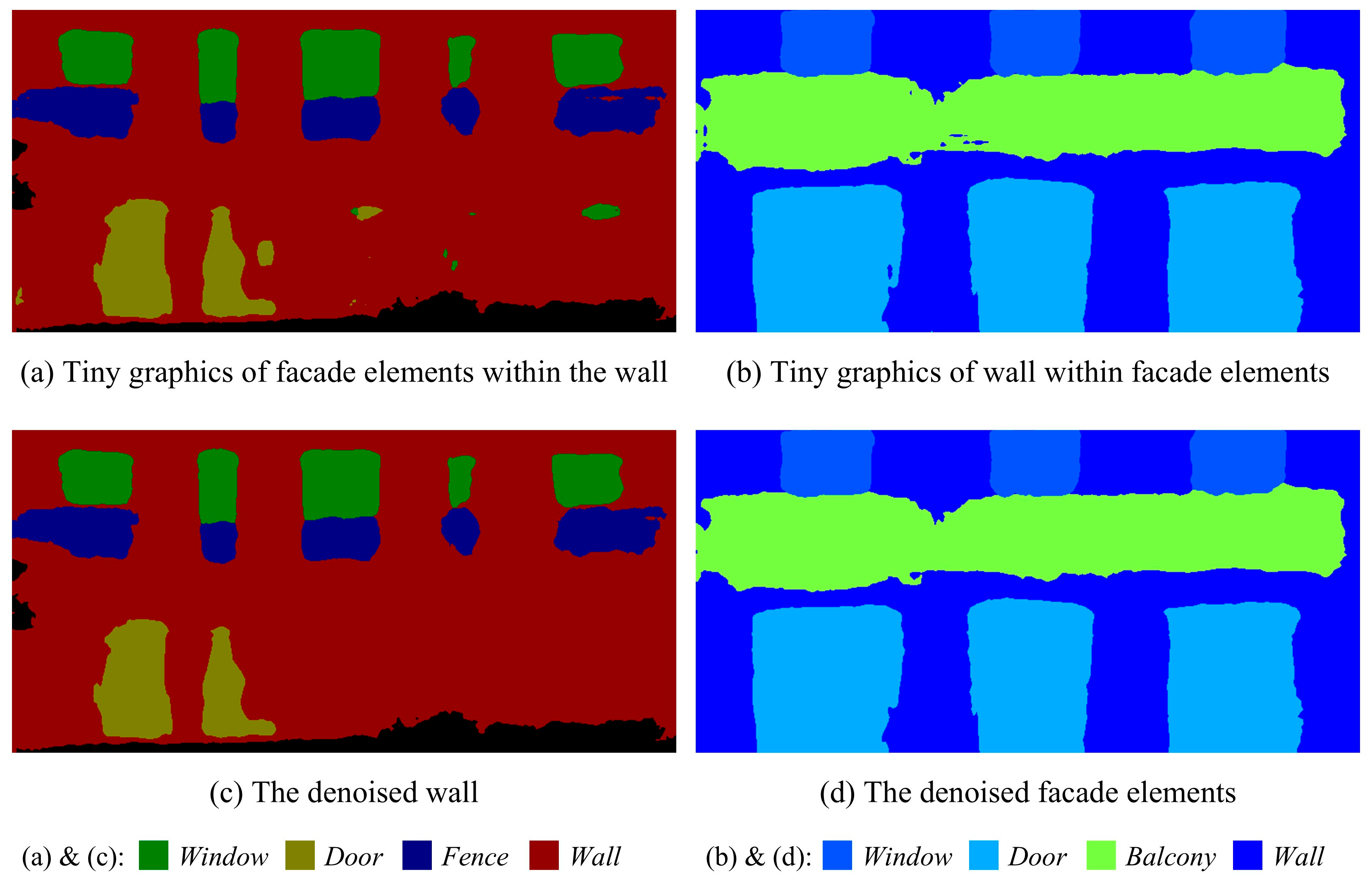
Noise in segmented facades typically manifests as discontinuous tiny graphics, resulting from insufficient differentiation in pixels’ class probabilities in the regions without distinct visual features. Specifically, there are two main types of noise, tiny graphics of facade elements within the wall and tiny graphics of wall within facade elements. The former presents as fragmented pixel clusters, as shown in Figure 7a. This type of noise would falsely introduce microscale elements that do not actually exist into the wall of regularized segmentation, adversely affecting the effect of regularization. The other type of noise emerges as holes within intact facade elements, as shown in Figure 7b. It significantly reduces the area of the MIB, thus increasing the coordinate differences between the boundaries of the MIB and MCB. Consequently, the efficiency of candidate box generation is greatly compromised.
To exclude the noise, two operations need to be performed on the raw prediction of facade segmentation. For the first type of noise, the graphics of facade elements with fewer than one-thousandth of the total image pixels are removed, as shown in Figure 7c. For the second type, if a hole lies entirely within a single graphic of facade element, fill the hole by changing the class of its constituent pixels to that of the enclosing graphic, as shown in Figure 7d.
Based on the denoised segmentation, regularization can be conducted more efficiently and effectively. Moreover, our strategies of candidate box generation (introduced in Definition 3 in Section 3.2) and BOB stacking (introduced in Section 3.3.3) can further mitigate the impact of noise due to their mechanisms.

3.3.2. BOB Finding

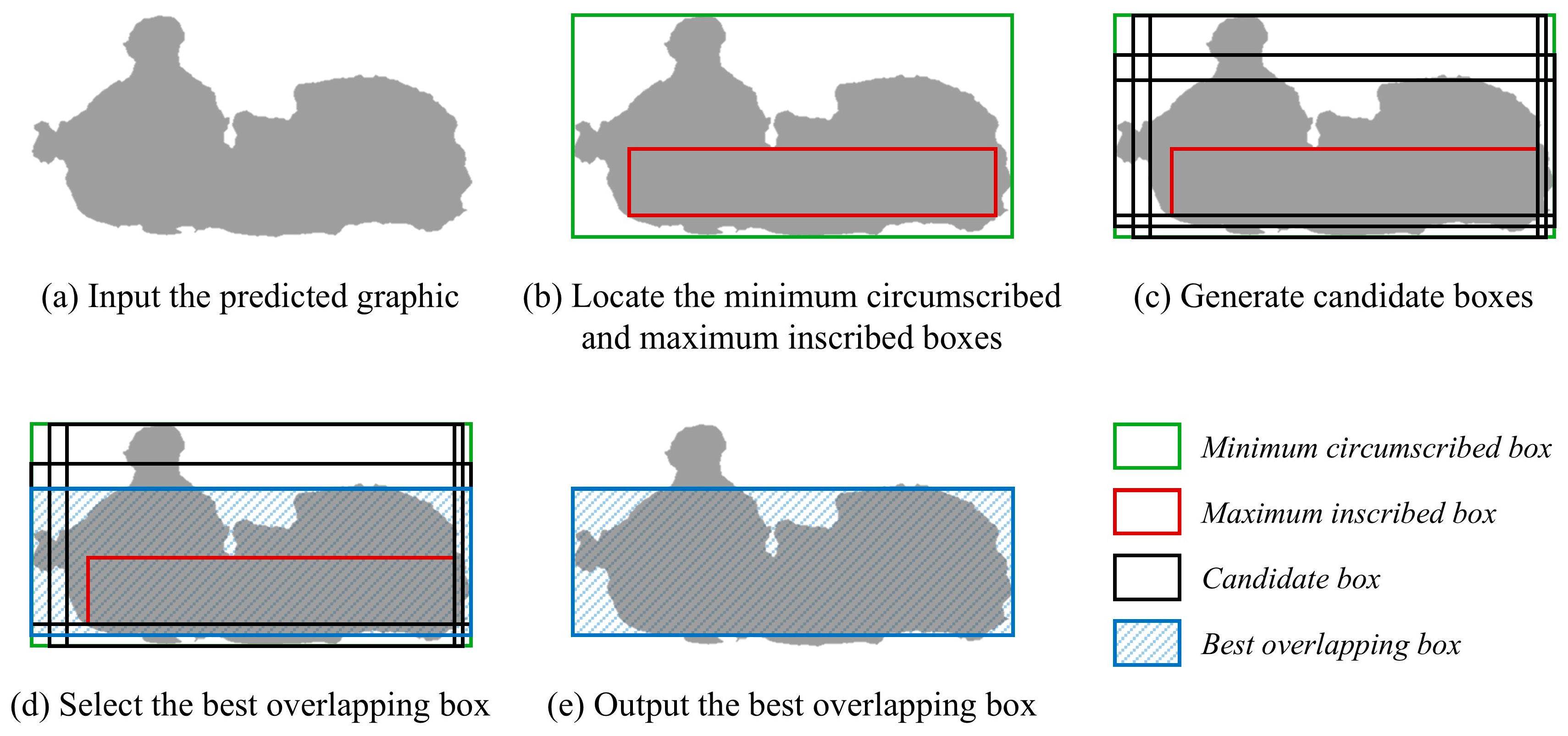
For each predicted graphic, its best overlapping box is found through the following steps by using the minimum circumscribed box, maximum inscribed box, and candidate boxes, as shown in Figure 8.
Step 1: Locate the minimum circumscribed box and maximum inscribed box of the predicted graphic.
Step 2: Generate candidate boxes and calculate the IoU between the predicted graphic and each candidate box.
Step 3: Select the candidate box that achieves the highest IoU with the predicted graphic as the best overlapping box.

3.3.3. BOB Stacking

After finding the BOB of all predicted graphics, the BOBs are stacked onto the same layer to replace the predicted graphics. According to principle 2, the IoU of the best overlapping box is negatively correlated with the degree to which the facade element is covered. Therefore, the BOBs are stacked according to the order of IoU from low to high. In other words, this order follows the covering relationship between facade elements.
In addition, part of the unannotated pixels in the low-IoU BOB would be covered by the high-IoU BOB stacked later, as shown in Figure 9. Considering that the operation of changing pixels’ predicted class is likely to make mistakes, and the high-IoU BOB executes less such operations than the low-IoU BOB, this order also helps to reduce the prediction’s correctness degradation caused by regularization.

3.4. Complexity

As shown in Algorithm 1, the time complexity of the proposed method is governed by six independent parameters, i.e., the number of facade images (NI), the number of graphics per image (NG), and the coordinate difference respectively between the left (DL = LMIBLMCB), bottom (DB = BMIBBMCB), right (DR = RMCBRMIB), and top (DT = TMCBTMIB) boundaries of the MCB and MIB per graphic. Since these parameters are organized into two quadruply nested for-loops, (NI × NG × DL × DR) and (NI × NG × DB × DT), the theoretical time complexity of the proposed method is O(N4). However, except for NI, all other parameters are bounded in practice. NG does not increase indefinitely as the number of elements is around dozens in most building facades. Benefitting from the advancement of semantic segmentation technology, DL, DB, DR, and DT would not increase with the input size but remain at a low level generally. Due to quantitative constraints, these five parameters can also be essentially considered constants. In other words, the actual complexity of our method primarily depends on only one parameter NI, making it equivalent to O(N) and computationally feasible. Experimental evidence that supports this claim is reported in detail in Section 4.4.3.

4. Experiment

To validate the effect of the proposed method, an experiment was conducted according to the procedure shown in Figure 10. First, we trained classifiers to segment building facade images, thereby obtaining real predicted graphics of facade elements. Second, several graphic regularization methods, including ours, were individually applied to regularize the predicted graphics. Third, the regularized graphics were compared and analyzed.

4.1. Data

To obtain the real predictions to regularize, we introduced four finely annotated datasets of facade segmentation, namely Irregular Facades (IRFs) [36], CMP Facade Database [37], ECP Paris [38], and ICG Graz50 [39]. The IRFs contain 1057 high-quality samples mainly of modern building facades, while there are 378, 104, and 50 classical facades in the CMP, ECP, and Graz50, respectively. Among diverse facade elements, we focused on those of the main classes that exist in most of the facades and with the most pixels, i.e., Window, Door, and Balcony. Note that the class Balcony is named Fence in the IRFs and is not included in the Graz50.
For each dataset, the predicted graphics of facade elements were obtained through a 10-fold cross-test approach as follows. First, the samples in the dataset were randomly partitioned into ten equal-sized folds. Second, a single fold was held out as the test set, while the remaining nine folds were combined for training and validation in the first round. A classifier was trained by a widely used network DeepLabv3+ [40] and applied to segment the facades in the test set. The training and segmentation were repeated ten rounds, with each fold used exactly once as the test set. Finally, the segmented facades in the ten test sets were combined. The predicted graphics of facade elements of the main classes were used as objects to regularize. Table 1 shows the hyperparameter settings.
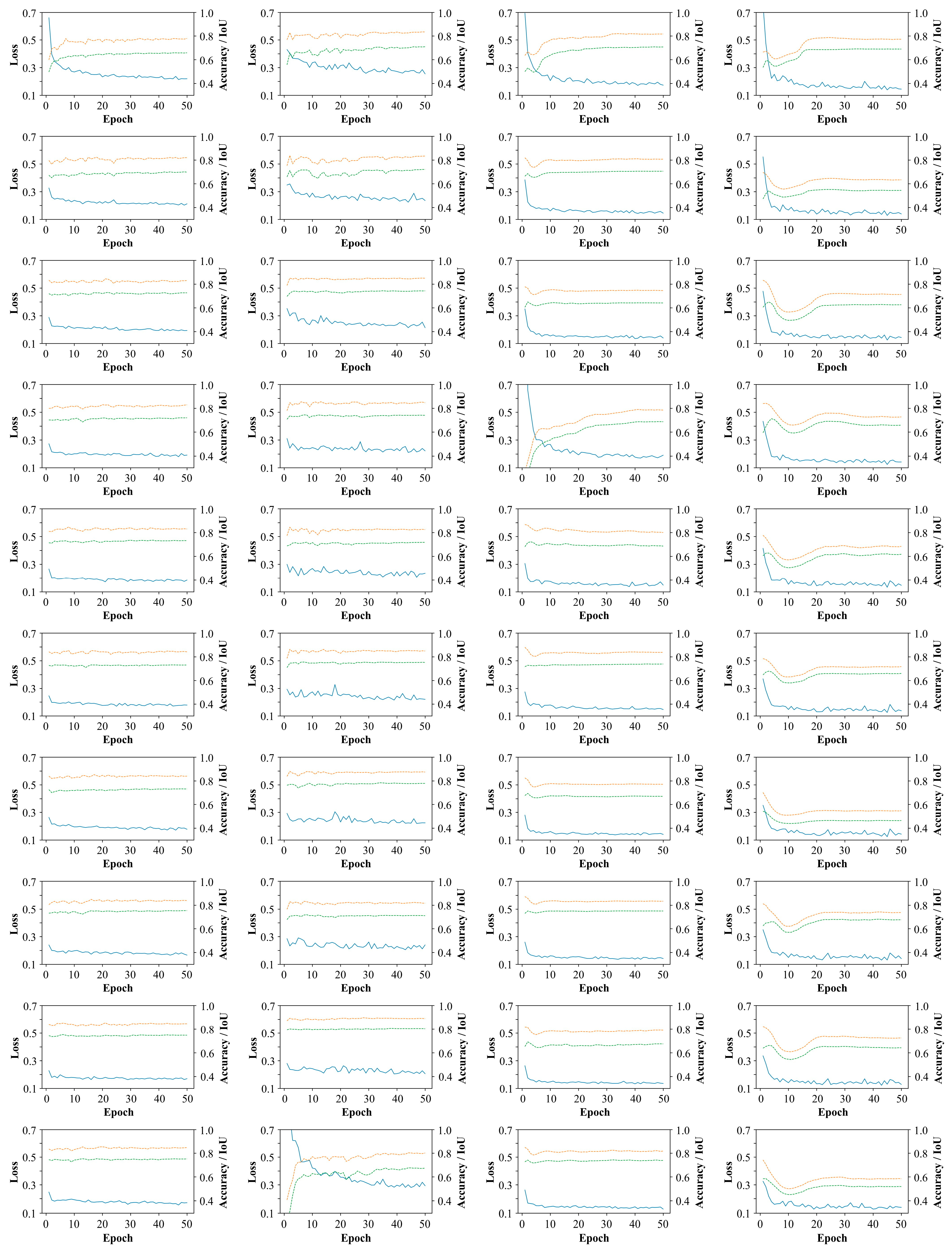
As shown in Figure 11, the training and validation curves across different rounds within the same dataset exhibit overall similarity, indicating low variation in segmentation quality and consequently enhancing the reliability of the evaluation of regularization effects. Across different datasets, the metrics exhibit certain variations, which help evaluate the stability of our method when applied to the predicted graphics of varying quality.

4.2. Methods

In addition to our box-based method, two axis-based regularization methods proposed by Du et al. [24] and Pan et al. [25] respectively were also adopted for comparison. Their methods regularize graphics to rectilinear polygons, though the polygons are not necessarily the basic shapes. The similar outputs make these methods comparable to ours. Each method was applied individually to regularize the predicted graphics.
Moreover, we also directly used the MCB and MIB to regularize the predicted graphics, respectively. The graphics regularized by them were then compared with those regularized by the BOB in ablation analysis.

4.3. Metrics

Intersection over Union (IoU) [41], the most used metric in related fields, was adopted as the main metric to measure the correctness of the predicted and regularized graphics. The calculation mechanism of IoU makes it very sensitive to the errors of pixel class. This helped to observe the differences in correctness between the graphics regularized by different methods. Besides IoU, F1-score that balances precision and recall was also adopted to assist the evaluation. For each image, the metrics were computed as:
I o U = T P T P + F P + F N
P r e c i s i o n = T P T P + F P
R e c a l l = T P T P + F N
F 1 = 2 · P r e c i s i o n · R e c a l l P r e c i s i o n + R e c a l l
where TP, FP, and FN represent the total number of pixels that were true positive, false positive, and false negative of the main class, respectively.
It should be noted that accuracy was not adopted in the experiment though it was also commonly used. Considering that the facade elements only took up a small part of the whole image, the large number of pixels of class Wall caused an abnormally high number of true negative (TN) pixels that were involved in the calculation of accuracy, thereby weakening the effectiveness of accuracy.

4.4. Results

The effect, correctness, and time consumption of the graphic regularization methods are reported in Section 4.4.1, Section 4.4.2 and Section 4.4.3, respectively, while Section 4.4.4 presents an ablation analysis of the boxes used in our method.

4.4.1. Effect

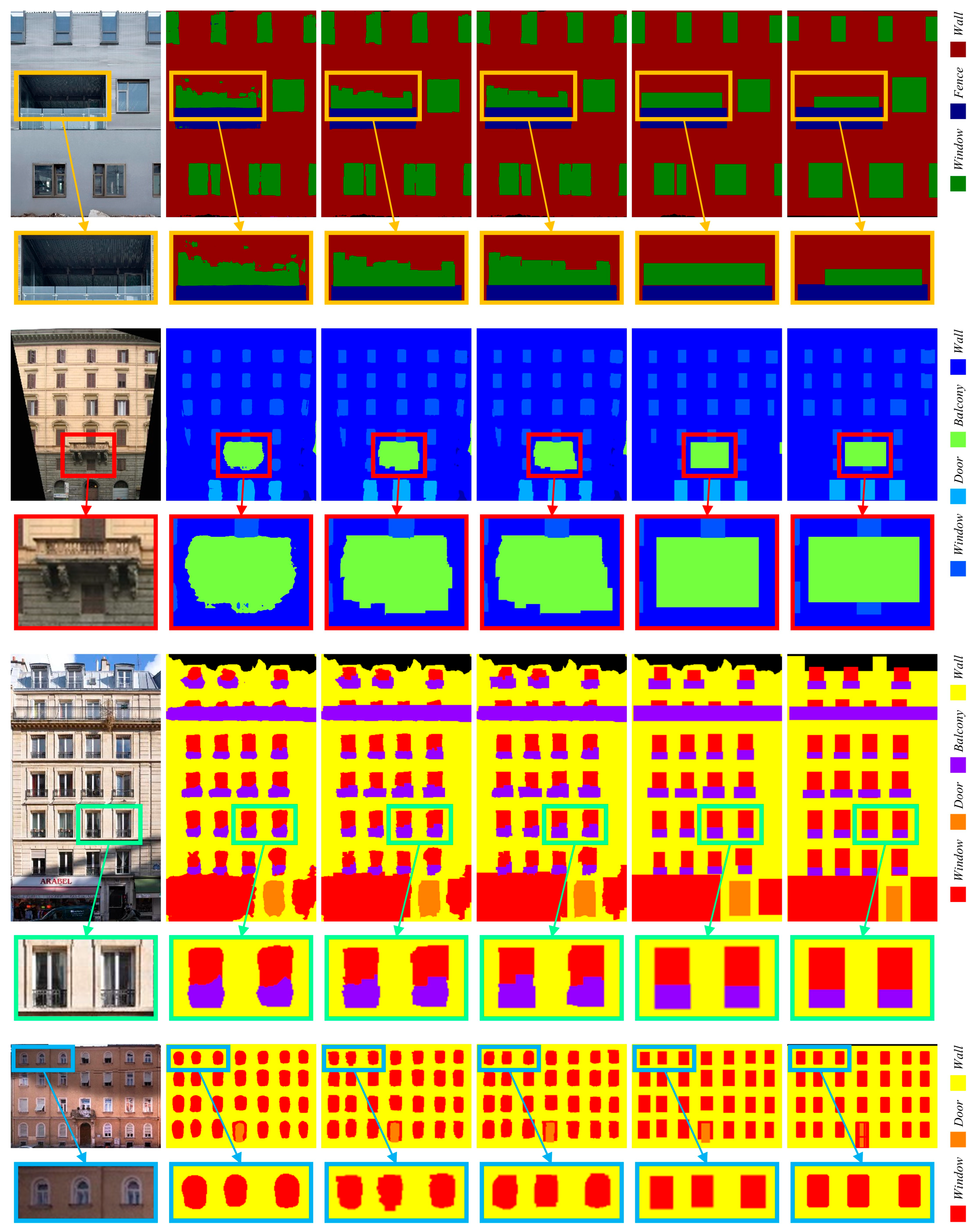
Figure 12 shows examples of the graphics regularized by each method. Compared with the regularizations of Du et al. and Pan et al., the graphics regularized by our method are more consistent with the ground truth in form. When focusing on shapes and edges, the graphics regularized by our method are more regular-shaped than those regularized by Du et al. and Pan et al. The edges of our regularization are also smoother than theirs. Compared with our regularizations, their regularizations exhibit significantly more pronounced aliasing, as highlighted in the colored boxes in Figure 12.
The difference in geometric characteristics of the regularized graphics comes from the different regularization mechanisms of the methods. The methods of Du et al. and Pan et al. do not assume that the shapes of the predicted graphics were supposed to be basic rectilinear polygons, instead attempt to approximate a relatively complex rectilinear polygon based on the predicted graphic’s edge. It does not mean that the methods of Du et al. and Pan et al. are worse than ours as they were originally devised for the prediction of other objects (e.g., building footprints). However, faced with the predicted graphics of facade elements, we can conclude safely that our method is the most appropriate one for the regularization task, as the graphics regularized by our method conform to the composition principle of most building facades better.

4.4.2. Correctness

Table 2 shows the IoU and F1-score of the predicted and regularized graphics. Compared with the predicted graphics, the graphics regularized by previous methods slightly lose some degree of correctness. This may be because regularization can only be performed based on the geometric properties of the predicted graphics, without relying on visual features in real-scene images. In contrast, since our method regularizes the predicted graphics based on both geometric properties and prior knowledge of facade composition, the correctness of the graphics regularized by our method is generally higher than, or at least not lower than, that of the predicted graphics. In other words, our method regularizes the predicted graphics of facade elements into basic rectilinear polygons without degradation in correctness.
To confirm whether the advantage is stable, we performed a two-tailed paired t-test on the metrics of the predicted and regularized graphics. The results show that the degradation in correctness of graphics regularized by the methods of Du et al. and Pan et al. is statistically significant across all metrics and datasets. For our method, two scenarios exist. When regularizing the predicted graphics of elements in classical facades, the accuracy of the regularized graphics is highly likely to improve, as shown in the metrics of the datasets CMP, ECP, and Graz50. For the dataset IRFs mainly of modern building facades, although the accuracy has not increased, it has not decreased.
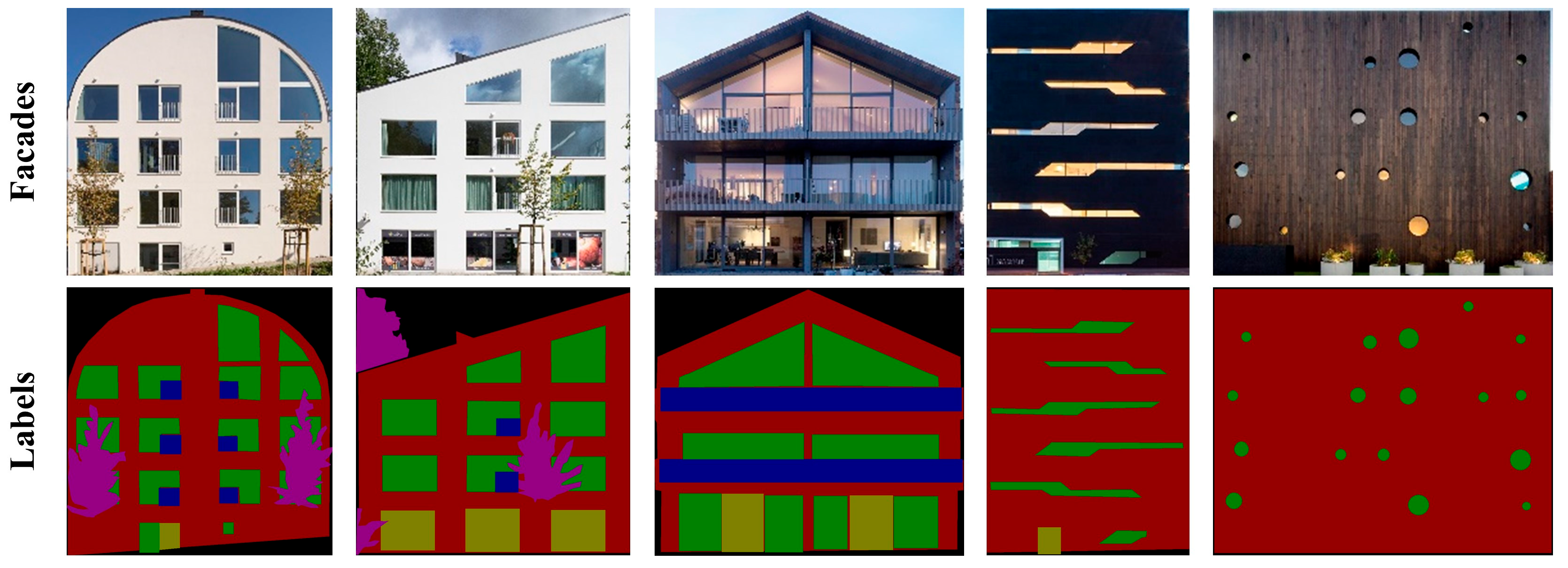
The number of non-basic-rectilinear elements, as shown in Table 3, may explain the different performance of our method between modern and classical facades. Compared with the datasets CMP, ECP, and Graz50, the dataset IRFs contains a greater number and a higher proportion of non-basic-rectilinear facade elements, as shown in Figure 13. This is considered the reason why our method underperforms in regularizing predicted graphics in modern facades compared to classical facades.
In summary, our method can regularize the predicted graphics of facade elements without degradation in correctness, which can be considered an advantage. This is more pronounced for classical architecture than for modern architecture.

4.4.3. Time Consumption

Table 4 and Table 5 show the time consumption of regularization at image- and graphic-level respectively. As shown in Table 4, our method took significantly more time on average to regularize an image compared to the methods of Du et al. and Pan et al. However, given that the absolute time required to process a single image is quite low, ranging from 0.36 to 1.65 s across different datasets, the total time consumption of our method remains acceptable. Even for the most time-consuming dataset IRFs, the proposed method can regularize 1057 images within half an hour (1739 s). Considering that computer vision tasks for building facades typically do not require high real-time performance, we believe that our method is feasible for practical applications.
By comparing the time consumption per image of our method and the number of graphics per image in Table 4 and Table 5, it can be observed that the dataset IRFs, which has the highest average time consumption per image for our method (1.65 s), contains the smallest number of graphics per image (17.3). Meanwhile, the dataset ECP, which has the highest average number of graphics per image (48.1), corresponds to only a moderate average time consumption per image (0.54 s). Similar trends are also observed in the time consumption of Du et al.’s and Pan et al.’s methods. This suggests that the time consumption of regularization depends more on the regularity of the predicted graphics, as datasets IRFs and ECP exhibit the highest (90.2 ms) and lowest (10.0 ms) average time consumption per graphic respectively, as shown in Table 5.
Table 6 and Table 7 count the average coordinate differences between the left, bottom, right, and top boundaries of the MCB and MIB per predicted graphic, supporting this suggestion. From an average perspective, the difference between the MCB and MIB of the IRFs’ graphics is the most significant. This explains why they require the highest average time consumption for regularization. For datasets ECP and Graz50, where the average differences between the MCB and MIB of predicted graphics are relatively similar, the gap in their time consumption per image is primarily due to the difference in the numbers of graphics per image.
It is worth noting that although the means of DL, DB, DR, and DT are all less than 10 across all datasets, the standard deviation and range are quite large. Since our method involves nested for loops, the time consumption may increase quadratically when regularizing graphics, for which the difference between the MCB and MIB is significant. However, since such large variations occur only in a small number of graphics—as supported by the median and 95% confidence intervals—their impact on the overall time consumption remains limited.
In summary, although our method is somewhat slower than previous methods for graphic regularization, its time consumption is entirely acceptable and feasible for real-world tasks.

4.4.4. Ablation Analysis

In the proposed method, for each predicted graphic, the best overlapping box (BOB) is found based on the minimum circumscribed box (MCB) and maximum inscribed box (MIB). All these boxes can convert irregular graphics into rectangles. This section evaluates whether the BOB yields better outputs compared to directly using the MCB or MIB. To achieve this goal, we calculated the metrics of the graphics regularized using MCB or MIB individually. The differences between these metrics and those of the BOB were also calculated and subjected to a two-tailed paired t-test.
As shown in Table 8, the BOB-regularized graphics show higher IoU than those regularized by the MCB or MIB across all datasets. In terms of precision and recall, the MIB and MCB performed the best, respectively. This aligns with expectations, as the MCB aims to maximize the inclusion of true positive (TP) pixels, whereas the MIB strives to minimize the inclusion of false positive (FP) pixels. However, this one-sided approach is unreliable. In this way, a lot of FP pixels could be incorrectly included by the MCB, while many TP pixels are excluded by the MIB. As a result, both MCB and MIB underperform BOB in F1-score that balances precision and recall.
The differences in the metrics are consistently observed across all datasets and show very strong statistical significance (p < 0.001), demonstrating that the BOB is necessary for achieving high-quality regularization of the predicted graphics of facade elements.

5. Discussion

In this study, we propose a box-based method that regularizes the predicted graphics of building facade elements by using the best overlapping box (BOB) that is defined based on the characteristics of facade composition logic. Compared with previous axis-based methods, the proposed method can convert irregular predicted graphics of facade elements into a more regular shape without degradation in correctness. This section further illustrates our method in three aspects.

5.1. Regularizing Predictions with Prior Knowledge

The core idea of this study is to regularize irregular predicted graphics based on both their geometric features and the prior knowledge of what they should be like. This is different from most previous methods that can be categorized as data-driven approaches. As this kind of method only focuses on the predicted graphic itself, regularization is limited to the optimization of several geometric characteristics, for example, the approximation of smooth outlines. However, without prior knowledge of regularization objects, it is uncertain whether the regularized graphics align well with the ground truth. By introducing prior knowledge, regularization can be guided from a model-driven perspective [42]. Specifically, the regularization target is directed to what the graphics actually be like based on the prior knowledge of building facade composition. The mixture of data- and model-driven approaches improves the effect and correctness of regularization [21].
In the past few years, some scholars have noticed the importance of prior knowledge for prediction regularization. Du et al. [24] and Pan et al. [25] analyzed the layout of buildings and found that most contour segments of building footprints are orthogonal to each other. Based on their findings, they adopted the constraints of orthogonality and main direction, respectively, to support the regularization, thereby improving the consistency between the regularized building footprints and their actual shapes. However, they did not further utilize the relationship between the contour segments, i.e., how the contour segments were organized. As a result, their methods were devised to be complex to adapt to the massive possible combinations of the contour segments. In contrast, the method proposed in this study regularizes the predicted graphics not only based on the geometric features of facade elements but also based on the relationship between the elements. As our method follows a few principles of the facade composition logic, it can regularize the predicted graphics of various facade elements through a very simple process. This suggests that the prior knowledge of regularization objects is valuable to both the results and the mechanism of regularization.
Kwak and Habib adopted a similar idea in their work [43]. Based on the morphological analysis of planar rooftops, they regarded the complex right-angled-corner buildings as a combination of rectangles of varying sizes and introduced the minimum bounding rectangle (MBR) as the basic operation of regularization. The role of MBR is similar to the BOB in this study. By generating a set of level-wise smaller MBRs, the real building shape was approximated recursively from the LiDAR point cloud. Essentially, this process can be described as repeating a simple operation until the ending condition is triggered. In other words, their work also supports our suggestion that the prior knowledge of regularization objects contributes to the simplification of regularization methods.

5.2. Comparison with Object Detection

To obtain regular predictions of facade elements, alongside the approach of graphic regularization, some scholars have also paid attention to the rectangular bounding boxes output by object detection. However, the precision of object detection is commonly inferior to that of semantic segmentation due to factors such as preset anchor sizes and inconsistent receptive fields [44]. Therefore, it is commonly combined with semantic segmentation to obtain regular and precisely predicted graphics. In this approach, an image of a building facade is fed into both a semantic segmentation network and an object detection network. By comparing the output pixel mask and bounding boxes, the most probable element locations and boundaries are inferred, ultimately yielding rectangular predictions of facade elements [45,46].
Fundamentally, these two approaches can be regarded as two distinct modes of optimization for semantic segmentation, the serial mode and the parallel mode, as shown in Figure 14.
For the parallel mode, semantic segmentation and object detection are executed simultaneously, jointly receiving input and producing output. They are interdependent and exhibit a high degree of coupling. In contrast, in the serial mode, graphic regularization is performed after semantic segmentation, with the output of semantic segmentation serving as its input. The coupling between semantic segmentation and graphic regularization is loose, allowing them to be flexibly decoupled into two independent tasks. As a result, the proposed method is not necessarily bound to specific semantic segmentation tasks. It can be flexibly integrated with the outputs of various facade segmentation tasks, and is compatible with different element types, sizes, aspect ratios, and composition patterns across architectural styles.
Moreover, our method can be considered a post-processing module for facade segmentation. Since it does not compromise the correctness of the predicted graphics, demonstrated by our experimental results, the final quality of regularized graphics depends solely on the performance of semantic segmentation. In other words, the regularization will be satisfactory as long as the segmentation performs well. This avoids the uncertainty associated with the performance of object detection.
Lastly, this simple yet effective method is easy to apply, not requiring specific conditions, such as image quality, sample amount, etc. Compared to the ever-expanding parameter scale of object detection networks, the low computational cost of our method enables its deployment on virtually any hardware platform.
In summary, the method proposed in this study is flexible, stable, and has low requirements for application conditions, making it well-suited for distributed application scenarios across diverse teams and tasks.

5.3. Future Applications

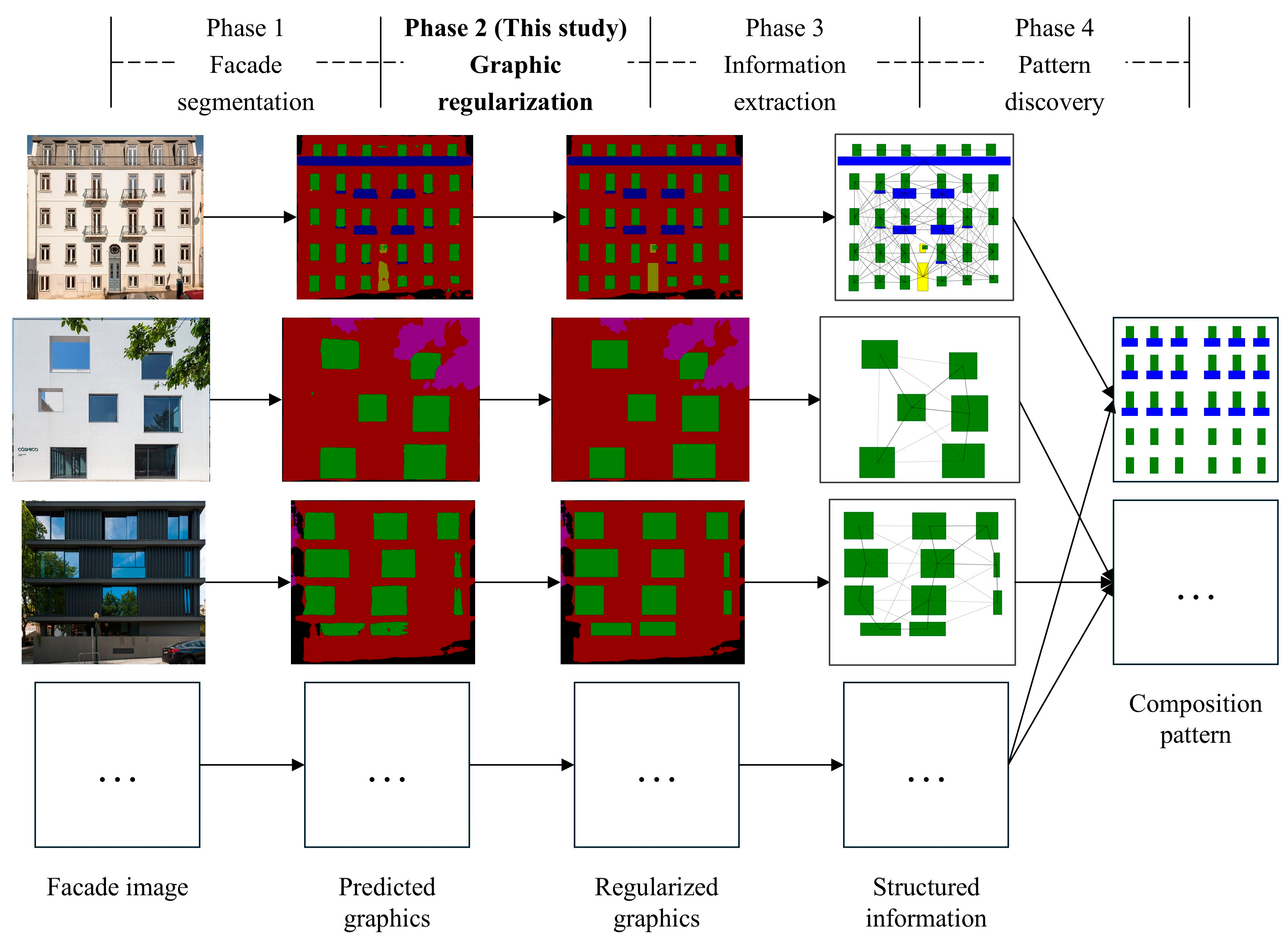
This work is a main part of the research project of data mining on building facade images, as shown in Figure 15. Based on the regularized prediction of facade segmentation, structured facade information can be extracted as graphs from which the composition patterns within specific scopes are discovered efficiently.
For researchers in theoretical fields such as architectural typology, aesthetics, and history, the discovered patterns can be considered objective evidence that supports the analysis of formal metatypes, pattern language, architectural context, etc. On the other hand, these patterns are also useful for architectural design. Architects are expected to deconstruct the existing patterns and reorganize the facade elements, thereby creating novel facade composition patterns reasonably.
In addition to the applications under the data mining framework, the proposed method can also provide direct support for many image-based tasks. These tasks include, but are not limited to, (i) 3-D building reconstruction, (ii) urban scene modeling, and (iii) facade assessment of energy consumption, lighting condition, accessibility, and visibility. As our method improves the quality of the output of semantic and instance segmentation, which is widely applied in many fields, more potential applications of this method may arise in the near future.

6. Limitations

The main limitation of this study is that our method can only regularize graphics into rectilinear polygons. However, there are also non-rectilinear shaped elements in building facades, e.g., circular windows. Restricting predicted graphics to rectilinear polygons may damage originally correctly identified non-rectilinear polygonal elements, thereby adversely affecting the correctness of the regularized graphics. Although such elements account for a small proportion of all facade elements, as shown in Table 3 in Section 4.4.2, their absolute number is not negligible. Considering the rapid growth of contemporary architecture, the freely designed facades further increase the number of non-rectilinear shaped elements. In the future, the proposed method must be upgraded to adapt the facade elements to more complex shapes.
Potential improvements may come from the following two perspectives. First, introduce a pre-classification step for the shape of predicted graphics and use different methods to regularize the predicted graphics in rectilinear and non-rectilinear classes, respectively. Second, predefine more bounding shapes and use the one with the highest probability to regularize the predicted graphic. Beyond these two perspectives, more ingenious strategies are also anticipated.
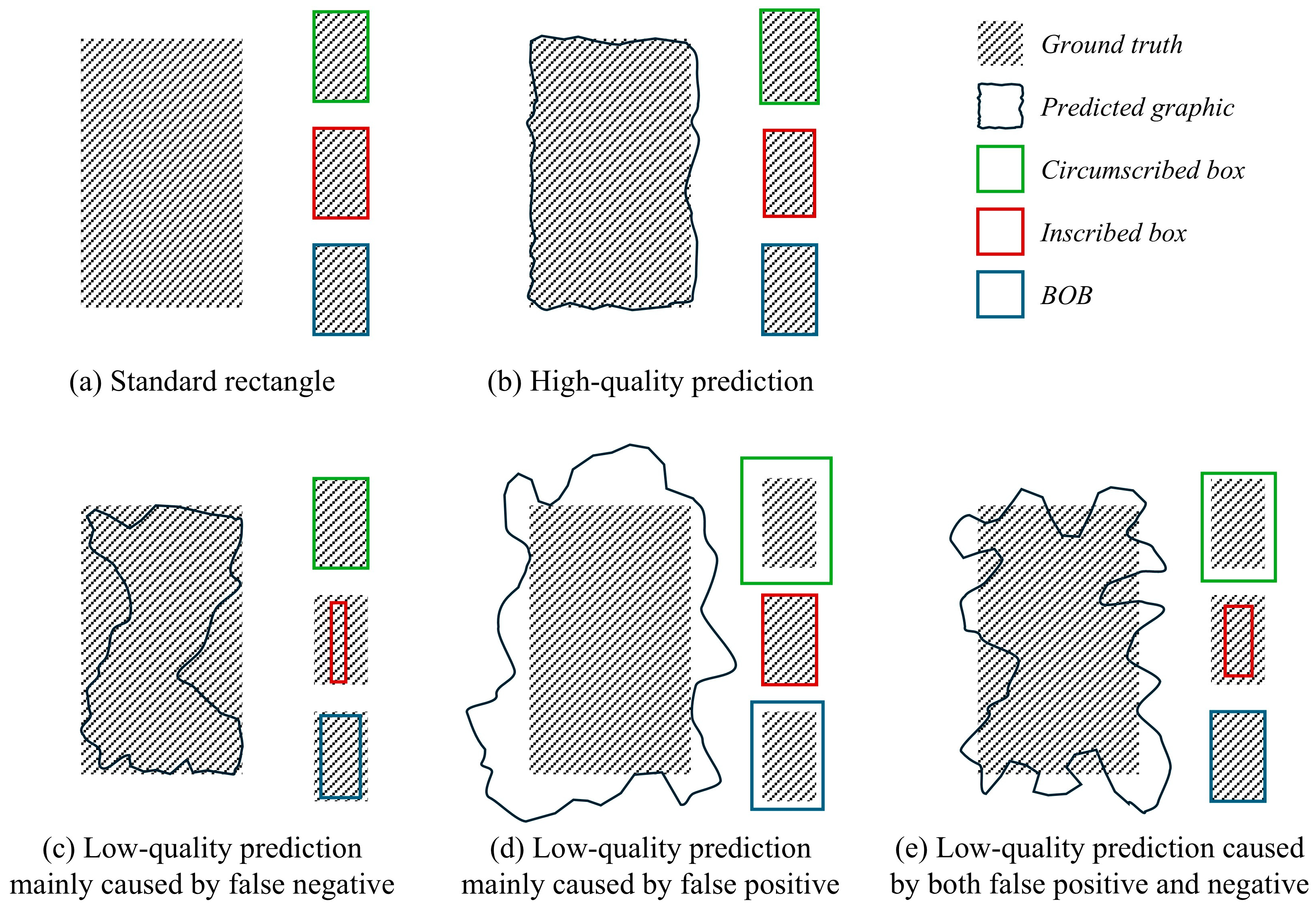
Another limitation is the exclusive use of best overlapping box (BOB), while minimum circumscribed box (MCB) or maximum inscribed box (MIB) may regularize the predicted graphics better in some cases. As shown in Figure 16a, for a standard rectangle, there is no difference between its MCB, MIB, and BOB. All these boxes overlap the rectangle perfectly. Faced with real predicted graphics, however, the effect of these boxes depends on the prediction’s quality. If the quality of prediction is high, the situation is similar to that of the standard rectangle, as shown in Figure 16b. The MCB, MIB, and BOB are all very close to the ground truth of the predicted graphic. On the contrary, for low-quality predictions, which box is more suitable for the regularization depends on the main error type of the predicted graphics. As shown in Figure 16c, if there are too many false negatives in the predicted graphic, the MCB would be closer to the ground truth than the MIB and BOB. In contrast, the MIB may become the best box for regularization when false positives account for a large proportion of the predicted graphic, as shown in Figure 16d. When false positives and negatives are balanced, the BOB performs better as shown in Figure 16e.
In this study, we use BOB in regularization because it is a balanced strategy. For most predicted graphics with both false positives and negatives, the BOB helps to approximate the ground truth more effectively. However, the predictions in which the errors are unbalanced, as shown in Figure 16c,d, cannot be ignored. In these cases, the MCB or MIB could be a better choice for regularization.
As the ablation analysis in Section 4.4.4 demonstrates, if we only use one type of box to regularize the predicted graphics, the BOB is better than the MCB and MIB. However, a mixed strategy that uses different boxes for each predicted graphic would make the regularized graphics more consistent with the ground truth. Considering that we cannot know the error types of a predicted graphic without ground truth in actual segmentation tasks, the prior knowledge of facade segmentation is considered a possible basis for reasonable applications of the boxes. By presuming the probable error types of the predicted graphics of facade elements based on prior knowledge, the BOB, MCB, and MIB are expected to be applied flexibly for each predicted graphic, thereby improving the correctness of the regularized graphics.
Finally, our method has much higher average time consumption than previous methods. At the scale of thousands of images, this processing speed is acceptable. However, for potential tasks involving tens of thousands or even hundreds of thousands of images, such as city information modeling for high-density metropolitan areas, the total time consumption of graphic regularization would become substantial. Besides, possible higher discrepancy between the MCB and MIB caused by lower segmentation quality would further amplify the speed disadvantage of our method. By optimizing the coordinate sliding stride for candidate box generation, this issue will be addressed in our future work.

7. Conclusions

The image-based studies and applications of building facades are gaining increasing attention from many intersectional fields. Benefitting from the progress of computer vision technology, the elements in building facades can be predicted as graphics that are composed of pixels of the same class. To further analyze and utilize the information of these elements, e.g., class, area, position, and shape, it is necessary to regularize the predicted graphics with irregular outlines.
Focusing on the composition characteristics of building facades, this study proposes a box-based method to regularize the predicted graphics of facade elements into basic rectilinear polygons, such as rectangular, L-, U-, and T-shapes. To achieve this goal, we defined four types of axis-aligned rectangular boxes as the tool of regularization, namely minimum circumscribed box (MCB), maximum inscribed box (MIB), candidate box (CB), and best overlapping box (BOB). Based on these boxes, a three-stage process of graphic regularization was established, consisting of denoising, BOB finding, and BOB stacking. An experiment on graphic regularization was conducted to compare the performance of our and previous methods. The results show that the graphics regularized by our method are more consistent with the actual shape of building facade elements. Moreover, our method achieves regularization without degradation in correctness, which is a prevalent shortcoming observed in previous methods.
The main contributions of this study can be summarized as follows.
First, this study provides a targeted method to regularize the prediction of semantic segmentation of building facades. It converts the predicted graphics of facade elements from irregular shapes to basic rectilinear polygons that meet the composition features of facade design, without degradation in correctness. The regularized graphics are useful for the fields of 3-D reconstruction, building information modeling, facade assessment, etc.
Second, in addition to the geometric properties of the predicted graphic, this study emphasizes the importance of the prior knowledge of regularization objects. The prior knowledge of building facade composition leads to a very simple yet effective mechanism of graphic regularization that can be performed and applied to other fields with similar conditions easily and flexibly.
This study also has several limitations. As our method can only convert graphics into rectilinear polygons, it is not applicable to the non-rectilinear elements, such as circular windows. Updates adaptable to increasingly diverse facade elements will be necessary. Besides, the regularization strategy depending on BOB only does not significantly improve the correctness of the predicted graphics. A strategy that hybridizes BOB, MCB, and MIB could potentially address this issue. Algorithm optimizations that further reduce the time complexity are also needed, as the current time consumption of our method is much higher than that of comparable methods.
In the big data era, a great number of building facade images are being captured and shared rapidly. These images carry valuable information about facade composition. By regularizing the predictions of facade segmentation, the composition information can be further refined and easier to extract. This is vital for the feasibility of image-based analysis and applications on buildings and cities. Based on the regularization of predicted graphics, topics such as how to identify composition axes and moduli, abstract composition rules, and even convert raster images of building facades into vector ones are worth exploring in the future.

Author Contributions

Conceptualization, S.L. and S.Z.; methodology, S.L., Z.W. and S.Z.; software, Z.W., Y.H. and X.Z.; validation, Z.W., Y.H. and X.Z.; formal analysis, S.L. and Z.W.; investigation, Z.W., Y.H. and X.Z.; resources, S.L.; data curation, Z.W., Y.H. and X.Z.; writing—original draft preparation, S.L.; writing—review and editing, S.L. and S.Z.; visualization, Z.W., Y.H. and X.Z.; supervision, S.L. and S.Z.; project administration, S.L. and S.Z.; funding acquisition, S.L., Y.H. and S.Z. All authors have read and agreed to the published version of the manuscript.

Funding

This research was funded by the National Natural Science Foundation of China [grant number 52108014], China Postdoctoral Science Foundation [grant number 2020M681565], the Postgraduate Research & Practice Innovation Program of Jiangsu Province [grant number KYCX23_1453], the Humanities and Social Science Fund of Ministry of Education of China [grant number 23YJC840039]; and the Social Science Foundation of Jiangsu Province [grant number 22SHC008].

Data Availability Statement

Our experimental data is openly available in Kaggle at https://www.kaggle.com/datasets/liushuyuu/the-regularized-graphics-of-facade-elements (accessed on 19 September 2025). The library DeepLabV3Plus-Pytorch is openly available in GitHub at https://github.com/VainF/DeepLabV3Plus-Pytorch (accessed on 4 July 2025).

Acknowledgments

The authors are grateful for the assistance from graduate student Junjie Wei, the samples from datasets IRFs, CMP Facade Database, ECP Paris, and ICG Graz50, and the code of DeepLabv3+ from library DeepLabV3Plus-Pytorch. They contributed a lot to obtaining the real predictions of building facade segmentation in the experiment.

Conflicts of Interest

The authors declare no conflicts of interest.

References

  1. He, J.; Wang, L.; Zhou, W.; Zhang, H.; Cui, X.; Guo, Y. Viewpoint assessment and recommendation for photographing architectures. IEEE Trans. Vis. Comput. Graph. 2019, 25, 2636–2649. [Google Scholar] [CrossRef]
  2. Liu, S.; Zou, G.; Zhang, S. A clustering-based method of typical architectural case mining for architectural innovation. J. Asian Arch. Build. Eng. 2020, 19, 71–89. [Google Scholar] [CrossRef]
  3. Demir, G.; Çekmiş, A.; Yeşilkaynak, V.B.; Unal, G. Detecting visual design principles in art and architecture through deep convolutional neural networks. Autom. Constr. 2021, 130, 103826. [Google Scholar] [CrossRef]
  4. Zhang, X.; Aliaga, D. RFCNet: Enhancing urban segmentation using regularization, fusion, and completion. Comput. Vis. Image Underst. 2022, 220, 103435. [Google Scholar] [CrossRef]
  5. Wang, B.; Zhang, J.; Zhang, R.; Li, Y.; Li, L.; Nakashima, Y. Improving facade parsing with vision transformers and line integration. Adv. Eng. Inform. 2024, 60, 102463. [Google Scholar] [CrossRef]
  6. Zhang, R.; Jing, M.; Lu, G.; Yi, X.; Shi, S.; Huang, Y.; Liu, L. Building element recognition with MTL-AINet considering view perspectives. Open Geosci. 2023, 15, 20220506. [Google Scholar] [CrossRef]
  7. Hou, J.; Zhou, J.; He, Y.; Hou, B.; Li, J. Automatic reconstruction of semantic façade model of architectural heritage. Herit. Sci. 2024, 12, 400. [Google Scholar] [CrossRef]
  8. Liu, Y.; Chua, D.K.; Yeoh, J.K. Automated engineering analysis of crack mechanisms on building façades using UAVs. J. Build. Eng. 2025, 103, 112176. [Google Scholar] [CrossRef]
  9. Gu, D.; Chen, W.; Lu, X. Automated assessment of wind damage to windows of buildings at a city scale based on oblique photography, deep learning and CFD. J. Build. Eng. 2022, 52, 104355. [Google Scholar] [CrossRef]
  10. Cao, J.; Metzmacher, H.; O’DOnnell, J.; Frisch, J.; Bazjanac, V.; Kobbelt, L.; van Treeck, C. Facade geometry generation from low-resolution aerial photographs for building energy modeling. Build. Environ. 2017, 123, 601–624. [Google Scholar] [CrossRef]
  11. Zhang, Y.; Deng, X.; Zhang, Y. Generation of sub-item load profiles for public buildings based on the conditional generative adversarial network and moving average method. Energy Build. 2022, 268, 112185. [Google Scholar] [CrossRef]
  12. Sewasew, Y.; Tesfamariam, S. Historic building information modeling using image: Example of port city Massawa, Eritrea. J. Build. Eng. 2023, 78, 107662. [Google Scholar] [CrossRef]
  13. Dai, M.; Ward, W.O.; Meyers, G.; Tingley, D.D.; Mayfield, M. Residential building facade segmentation in the urban environment. Build. Environ. 2021, 199, 107921. [Google Scholar] [CrossRef]
  14. Hu, Y.; Wei, J.; Zhang, S.; Liu, S. FDIE: A graph-based framework for extracting design information from annotated building facade images. J. Asian Arch. Build. Eng. 2024, 24, 2530–2553. [Google Scholar] [CrossRef]
  15. Lotte, R.G.; Haala, N.; Karpina, M.; Aragão, L.E.O.e.C.d.; Shimabukuro, Y.E. 3D Façade Labeling over Complex Scenarios: A Case Study Using Convolutional Neural Network and Structure-From-Motion. Remote Sens. 2018, 10, 1435. [Google Scholar] [CrossRef]
  16. Zhao, K.; Kang, J.; Jung, J.; Sohn, G. Building extraction from satellite images using Mask R-CNN with building boundary regularization. In Proceedings of the IEEE Computer Society Conference on Computer Vision and Pattern Recognition Workshops, Salt Lake City, UT, USA, 18–22 June 2018; pp. 242–246. [Google Scholar]
  17. Kong, L.; Qian, H.; Xie, L.; Huang, Z.; Qiu, Y.; Bian, C. Multilevel regularization method for building outlines extracted from high-resolution remote sensing images. Appl. Sci. 2023, 13, 12599. [Google Scholar] [CrossRef]
  18. Wei, S.; Ji, S.; Lu, M. Toward automatic building footprint delineation from aerial images using CNN and regularization. IEEE Trans. Geosci. Remote Sens. 2020, 58, 2178–2189. [Google Scholar] [CrossRef]
  19. Douglas, D.H.; Peucker, T.K. Algorithms for the reduction of the number of points required to represent a digitized line or its caricature. Cartogr. Int. J. Geogr. Inf. Geovis. 1973, 10, 112–122. [Google Scholar] [CrossRef]
  20. Liu, J.; Zhang, J.; Xu, F.; Huang, Z.; Li, Y. Adaptive algorithm for automated polygonal approximation of high spatial resolution remote sensing imagery segmentation contours. IEEE Trans. Geosci. Remote Sens. 2014, 52, 1099–1106. [Google Scholar] [CrossRef]
  21. Mousa, Y.A.; Helmholz, P.; Belton, D.; Bulatov, D. Building detection and regularisation using DSM and imagery information. Photogramm. Rec. 2019, 34, 85–107. [Google Scholar] [CrossRef]
  22. Wu, J.-S.; Leou, J.-J. New polygonal approximation schemes for object shape representation. Pattern Recognit. 1993, 26, 471–484. [Google Scholar] [CrossRef]
  23. Wang, S.; Yang, Y.; Chang, J.; Gao, X. Optimization of building contours by classifying high-resolution images. Laser Optoelectron. Prog. 2020, 57, 022801. (In Chinese) [Google Scholar] [CrossRef]
  24. Du, J.; Chen, D.; Wang, R.; Peethambaran, J.; Mathiopoulos, P.T.; Xie, L.; Yun, T. A novel framework for 2.5-D building contouring from large-scale residential scenes. IEEE Trans. Geosci. Remote Sens. 2019, 57, 4121–4145. [Google Scholar] [CrossRef]
  25. Pan, M.; Chang, J.; Gao, X.; Yang, Y.; Zhong, K. Building contour optimization method based on main direction. Acta Opt. Sin. 2022, 42, 5892. (In Chinese) [Google Scholar] [CrossRef]
  26. Li, X.; Qiu, F.; Shi, F.; Tang, Y. A recursive hull and signal-based building footprint generation from airborne LiDAR data. Remote Sens. 2022, 14, 5892. [Google Scholar] [CrossRef]
  27. Chen, Q.; Wang, L.; Waslander, S.L.; Liu, X. An end-to-end shape modeling framework for vectorized building outline generation from aerial images. ISPRS J. Photogramm. Remote Sens. 2020, 170, 114–126. [Google Scholar] [CrossRef]
  28. Zhao, H.; Shi, J.; Qi, X.; Wang, X.; Jia, J. Pyramid scene parsing network. In Proceedings of the 2017 IEEE Conference on Computer Vision and Pattern Recognition, Honolulu, HI, USA, 21–26 July 2017; pp. 2881–2890. [Google Scholar] [CrossRef]
  29. Kass, M.; Witkin, A.; Terzopoulos, D. Snakes: Active contour models. Int. J. Comput. Vis. 1988, 1, 321–331. [Google Scholar] [CrossRef]
  30. Menet, S.; Saint-Marc, P.; Medioni, G. Active contour models: Overview, implementation and applications. In Proceedings of the 1990 IEEE International Conference on Systems, Man, and Cybernetics Conference Proceedings, Los Angeles, CA, USA, 4–7 November 1990; pp. 194–199. [Google Scholar] [CrossRef]
  31. Brigger, P.; Hoeg, J.; Unser, M. B-spline snakes: A flexible tool for parametric contour detection. IEEE Trans. Image Process. 2000, 9, 1484–1496. [Google Scholar] [CrossRef]
  32. Velut, J.; Benoit-Cattin, H.; Odet, C. Locally regularized smoothing B-snake. EURASIP J. Adv. Signal Process. 2007, 2007, 076241. [Google Scholar] [CrossRef]
  33. Xu, C.; Prince, J.L. Snakes, shapes, and gradient vector flow. IEEE Trans. Image Process. 1998, 7, 359–369. [Google Scholar] [CrossRef]
  34. Xu, C.; Prince, J.L. Generalized gradient vector flow external forces for active contours. Signal Process. 1998, 71, 131–139. [Google Scholar] [CrossRef]
  35. Chang, J.; Gao, X.; Yang, Y.; Wang, N. Object-oriented building contour optimization methodology for image classification results via generalized gradient vector flow snake model. Remote Sens. 2021, 13, 2406. [Google Scholar] [CrossRef]
  36. Wei, J.; Hu, Y.; Zhang, S.; Liu, S. Irregular Facades: A dataset for semantic segmentation of the free facade of modern buildings. Buildings 2024, 14, 2602. [Google Scholar] [CrossRef]
  37. Tylecek, R. The CMP Facade Database (Version 1.1); Czech Technical University in Prague: Prague, Czech Republic, 2013; Research Report CTU-CMP-2012-24. [Google Scholar]
  38. Teboul, O.; Simon, L.; Koutsourakis, P.; Paragios, N. Segmentation of building facades using procedural shape priors. In Proceedings of the 2010 IEEE Computer Society Conference on Computer Vision and Pattern Recognition, San Francisco, CA, USA, 13–18 June 2010; pp. 3105–3112. [Google Scholar]
  39. Riemenschneider, H.; Krispel, U.; Thaller, W.; Donoser, M.; Havemann, S.; Fellner, D.; Bischof, H. Irregular lattices for complex shape grammar facade parsing. In Proceedings of the 2012 IEEE Conference on Computer Vision and Pattern Recognition, Providence, RI, USA, 16–21 June 2012; pp. 1640–1647. [Google Scholar]
  40. Chen, L.-C.; Zhu, Y.; Papandreou, G.; Schroff, F.; Adam, H. Encoder-decoder with atrous separable convolution for semantic image segmentation. In Proceedings of the European Conference on Computer Vision, Munich, Germany, 8–14 September 2018; pp. 833–851. [Google Scholar] [CrossRef]
  41. Jaccard, P. The distribution of the flora in the alpine zone. New Phytol. 1912, 11, 37–50. [Google Scholar] [CrossRef]
  42. Yu, W.; Shu, J.; Yang, Z.; Ding, H.; Zeng, W.; Bai, Y. Deep learning-based pipe segmentation and geometric reconstruction from poorly scanned point clouds using BIM-driven data alignment. Autom. Constr. 2025, 173, 106071. [Google Scholar] [CrossRef]
  43. Kwak, E.; Habib, A. Automatic representation and reconstruction of DBM from LiDAR data using Recursive Minimum Bounding Rectangle. ISPRS J. Photogramm. Remote Sens. 2014, 93, 171–191. [Google Scholar] [CrossRef]
  44. Neuhausen, M.; König, M. Automatic window detection in facade images. Autom. Constr. 2018, 96, 527–539. [Google Scholar] [CrossRef]
  45. Liu, H.; Xu, Y.; Zhang, J.; Zhu, J.; Li, Y.; Hoi, S.C.H. DeepFacade: A Deep Learning Approach to Facade Parsing With Symmetric Loss. IEEE Trans. Multimedia 2020, 22, 3153–3165. [Google Scholar] [CrossRef]
  46. Zhang, G.; Pan, Y.; Zhang, L. Deep learning for detecting building façade elements from images considering prior knowledge. Autom. Constr. 2022, 133, 104016. [Google Scholar] [CrossRef]
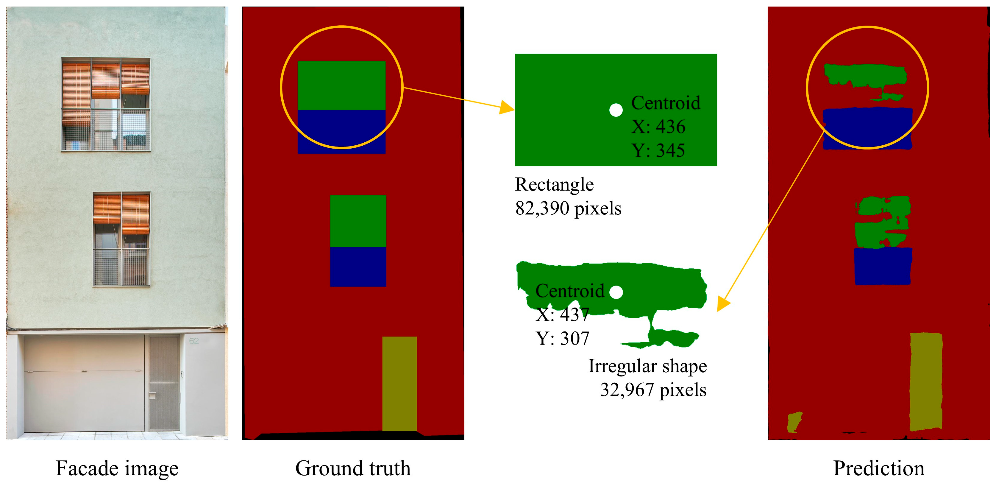
Figure 1. Information errors caused by irregular predictions. The colors green, yellow, blue, and red represent windows, doors, fences, and walls, respectively.
Buildings 15 03562 g001
Figure 2. The orthogonal composition of building facade.
Buildings 15 03562 g002
Figure 3. Examples of the composition logic of non-rectangular facade elements.
Buildings 15 03562 g003
Figure 4. Examples of the highest achievable IoU of the predicted graphic in different shapes.
Buildings 15 03562 g004
Figure 5. Diagram of the boxes used in this study.
Buildings 15 03562 g005
Figure 6. The process of regularization.
Buildings 15 03562 g006
Figure 7. Two types of noise and denoising operations.
Buildings 15 03562 g007
Figure 8. The mechanism of BOB finding.
Buildings 15 03562 g008
Figure 9. The mechanism of BOB stacking. The colors green and blue represent facade elements in the background and in the foreground, respectively.
Buildings 15 03562 g009
Figure 10. The experimental procedure [24,25].
Buildings 15 03562 g010
Figure 11. Learning curves of classifier training. (left to right) IRFs, CMP Facade Database, ECP Paris, and ICG Graz50; (top to bottom) round 1 to 10. Blue solid lines represent the training loss, while orange and green dashed lines respectively represent the accuracy and IoU on validation set.
Buildings 15 03562 g011
Figure 12. Examples of the regularized graphics. (left to right) image, prediction, Du et al.’s regularization, Pan et al.’s regularization, our regularization, and ground truth; (top to bottom) IRFs, CMP Facade Database, ECP Paris, and ICG Graz50.
Buildings 15 03562 g012
Figure 13. Examples of the facades with non-basic-rectilinear elements. The colors green, yellow, blue, red, and purple represent windows, doors, fences, walls, and plants, respectively.
Buildings 15 03562 g013
Figure 14. Two modes of obtaining regular annotations from facade images.
Buildings 15 03562 g014
Figure 15. The framework of data mining on building facade images. The colors green, yellow, blue, red, and purple represent windows, doors, fences, walls, and plants, respectively.
Buildings 15 03562 g015
Figure 16. Applicable situations for different boxes.
Buildings 15 03562 g016
Table 1. Hyperparameter settings for training.
HyperparameterDescription
network = “DeepLabv3+”The network DeepLabv3+ was used to train classifiers.
backbone = “MobileNet”The backbone for DeepLabv3+ was MobileNet.
batch_size = 16Parameters were updated every time 16 samples were input.
epochs = 50The training ran for 50 epochs.
learning_rate = 0.01The update to parameters is 0.01 times the gradient.
crop_size = 513Input images were resized to 513 × 513 pixels.
random_seed = 1-
Table 2. Correctness of the predicted and regularized graphics.
IoU F1
DatasetGraphicMeanSD95% CI MeanSD95% CI
IRFsPrediction0.7220.1470.713–0.731 0.8280.1250.821–0.836
Du et al.’s reg0.715 ***0.1480.706–0.724 0.823 ***0.1270.815–0.831
Pan et al.’s reg0.715 ***0.1500.706–0.724 0.823 ***0.1280.815–0.831
Our reg0.7230.1510.714–0.732 0.8280.1290.820–0.836
CMPPrediction0.7070.1030.697–0.717 0.8240.0750.816–0.831
Du et al.’s reg0.702 ***0.1050.692–0.713 0.820 ***0.0770.813–0.828
Pan et al.’s reg0.705 *0.1060.694–0.715 0.822 *0.0780.814–0.830
Our reg0.718 ***0.1060.708–0.729 0.831 ***0.0770.824–0.839
ECPPrediction0.7130.0880.696–0.730 0.8290.0680.816–0.842
Du et al.’s reg0.700 ***0.0900.683–0.717 0.820 ***0.0700.806–0.834
Pan et al.’s reg0.692 ***0.0940.674–0.710 0.814 ***0.0760.799–0.828
Our reg0.730 ***0.0850.713–0.746 0.841 ***0.0650.828–0.853
Graz50Prediction0.6370.0960.611–0.664 0.7740.0810.751–0.796
Du et al.’s reg0.629 ***0.0920.604–0.655 0.768 **0.0780.747–0.790
Pan et al.’s reg0.631 *0.0930.605–0.657 0.769 *0.0790.747–0.791
Our reg0.651 ***0.0970.624–0.678 0.784 ***0.0810.761–0.806
Note: reg, SD and 95% CI represent regularization, standard deviation and 95% confidence interval, respectively. Blue indicates values that are higher than or equal to that of prediction, while red indicates values that are lower than that of prediction. *, **, and *** denote a p-value of the two-tailed paired t-test that is <0.05, <0.01, and <0.001, respectively.
Table 3. The number of non-basic-rectilinear elements in the experiment.
DatasetNNNTNN/NTNFNN/NF
IRFs132418,2360.07210571.253
CMP6911,8950.0063780.183
ECP0500701040
Graz50010940500
Note: NN, NT, and NF represent the number of non-basic-rectilinear facade elements, the total number of facade elements, and the number of facades, respectively.
Table 4. Overall time consumption of regularization.
Total Time (s) Time per Image (s)
DatasetNimageDu et al.Pan et al.Ours Du et al.Pan et al.Ours
IRFs10573763041739 0.360.291.65
CMP37813692424 0.360.241.12
ECP104331356 0.320.130.54
Graz50506218 0.120.040.36
Table 5. The number of graphics per image and time consumption per graphic of our method.
Number of Graphics per Image Time Consumption per Graphic (ms)
DatasetMeanMedianSDRange95% CI MeanMedianSDRange95% CI
IRFs17.311.017.50–12416.2–18.3 90.219.01246.02.5–110,461.172.2–108.3
CMP31.529.017.45–14929.7–33.2 32.59.9276.92.7–24,162.027.6–37.5
ECP48.146.510.627–8446.1–50.2 10.05.223.12.1–604.89.3–10.6
Graz5021.922.05.910–3420.3–23.5 14.87.749.82.1–1321.311.8–17.7
Note: SD and 95% CI represent standard deviation and 95% confidence interval, respectively.
Table 6. Horizontal coordinate differences between the MCB and MIB per graphic.
DL (Pixel) DR (Pixel)
DatasetMeanMedianSDRange95% CI MeanMedianSDRange95% CI
IRFs5.4218.70–13155.1–5.7 5.5216.40–6945.3–5.8
CMP3.3113.60–6343.0–3.5 3.2112.50–7483.0–3.5
ECP1.913.40–821.8–2.0 1.713.60–751.6–1.8
Graz501.611.70–241.5–1.7 1.612.50–411.5–1.8
Note: DL represents the coordinate difference between the left boundaries of the MCB and MIB, and DR represents the coordinate difference between the right boundaries of the MCB and MIB. SD and 95% CI represent standard deviation and 95% confidence interval, respectively.
Table 7. Vertical coordinate differences between the MCB and MIB per graphic.
DB (Pixel) DT (Pixel)
DatasetMeanMedianSDRange95% CI MeanMedianSDRange95% CI
IRFs4.5210.40–3474.3–4.6 4.229.10–2664.1–4.3
CMP2.716.20–2522.6–2.8 2.717.40–2462.6–2.9
ECP1.311.80–301.2–1.3 2.113.90–722.0–2.2
Graz502.012.80–441.8–2.2 2.022.10–281.8–2.1
Note: DB represents the coordinate difference between the bottom boundaries of the MCB and MIB, and DT represents the coordinate difference between the top boundaries of the MCB and MIB. SD and 95% CI represent standard deviation and 95% confidence interval, respectively.
Table 8. Overall time consumption of regularization of the three types of boxes.
DatasetBoxIoUPrecisionRecallF1
BOB0.7230.8470.8180.828
IRFsMCB0.711 (−0.012) ***0.782 (−0.065) ***0.871 (+0.053) ***0.820 (−0.008) ***
MIB0.633 (−0.090) ***0.902 (+0.055) ***0.671 (−0.147) ***0.762 (−0.066) ***
BOB0.7180.8380.8300.831
CMPMCB0.682 (−0.036) ***0.745 (−0.093) ***0.887 (+0.057) ***0.805 (−0.026) ***
MIB0.665 (−0.053) ***0.923 (+0.085) ***0.700 (−0.130) ***0.792 (−0.039) ***
BOB0.7300.8270.8570.841
ECPMCB0.673 (−0.057) ***0.729 (−0.098) ***0.892 (+0.035) ***0.802 (−0.039) ***
MIB0.663 (−0.067) ***0.904 (+0.077) ***0.709 (−0.148) ***0.792 (−0.049) ***
BOB0.6510.7660.8070.784
Graz50MCB0.629 (−0.022) ***0.698 (−0.068) ***0.859 (+0.052) ***0.768 (−0.016) ***
MIB0.569 (−0.082) ***0.862 (+0.096) ***0.621 (−0.186) ***0.719 (−0.065) ***
Note: BOB, MCB and MIB represent the best overlapping box, minimum circumscribed box, and maximum inscribed box, respectively. Bold indicates the highest values. The values in parentheses represent variations compared with the metric of BOB. *** denotes a p-value of the two-tailed paired t-test that is <0.001.
Disclaimer/Publisher’s Note: The statements, opinions and data contained in all publications are solely those of the individual author(s) and contributor(s) and not of MDPI and/or the editor(s). MDPI and/or the editor(s) disclaim responsibility for any injury to people or property resulting from any ideas, methods, instructions or products referred to in the content.