A Two-Stage Hybrid Modeling Strategy for Early-Age Concrete Temperature Prediction Using Decoupled Physical Processes

Abstract

Predicting early-age temperature evolution in mass concrete is crucial for controlling thermal cracks. This process involves two distinct physical stages: an initial, hydration-driven heating stage (Stage I) and a subsequent, environment-dominated cooling stage (Stage II). To address this challenge, we propose a novel two-stage hybrid modeling strategy that decouples the underlying physical processes. This approach was developed and validated using a 450-h on-site monitoring dataset. For the deterministic heating phase (Stage I), we employed polynomial regression. For the subsequent stochastic cooling phase (Stage II), a Random Forest algorithm was used to model the complex environmental interactions. The proposed hybrid model was benchmarked against several alternatives, including a physics-based finite element model (FEM) and a single Random Forest model. During the critical cooling stage, our approach demonstrated superior performance, achieving a Root Mean Square Error (RMSE) of $0.24°\mathrm{C}$. This represents a 17.2% improvement over the best-performing single model. Furthermore, cumulative error analysis indicated that the hybrid model maintained a stable and unbiased prediction trend throughout the monitoring period. This addresses a key weakness in single-stage models, where underlying phase-specific errors can accumulate and lead to long-term drift. The proposed framework offers an accurate, robust, and transferable paradigm for modeling other complex engineering processes that exhibit distinct multi-stage characteristics.

1. Introduction

Owing to its superior load-bearing capacity and durability, mass concrete plays an indispensable role in large-scale infrastructure construction, including bridges, dams, and the foundations of high-rise buildings [1,2,3]. However, the substantial heat released during cement hydration leads to sharp internal temperature increases, followed by cooling and contraction due to environmental effects [4,5,6]. The temperature difference between the interior and exterior of the concrete induces thermal stress. If this stress exceeds the concrete’s early-age tensile strength, thermal cracks will initiate. These cracks impair structural integrity, accelerate steel corrosion, and pose severe threats to the structure’s safety and service life [7,8]. Therefore, accurately predicting early-age temperature fields in mass concrete is essential. This prediction is a prerequisite for implementing effective temperature control measures and preventing crack formation [9,10,11].

Early-age thermal cracking is a critical concern for large bridge projects, such as the one examined in this study. The structure’s massive concrete volume and subtropical location make it especially prone to such damage. A fundamental limitation of traditional prediction methods is their assumption of a single, homogeneous thermal process. However, the governing physics is distinctly two-stage: an initial, hydration-driven heating phase [12,13] followed by an environment-dominated cooling phase [14,15,16]. Ignoring this duality can lead to the accumulation of phase-specific errors [17,18,19]. This highlights the need for a modelling strategy that explicitly accounts for this phased transition.

Two mainstream prediction methods have been developed to address this challenge [13,20,21]. The finite element method (FEM), based on first principles, simulates temperature evolution by solving heat conduction equations with solid theoretical foundations [22,23,24]. However, FEM predictive accuracy depends heavily on the precise determination of material thermal parameters and the idealized treatment of complex boundary conditions [25,26,27]. Environmental factors such as solar radiation, wind speed, and precipitation are highly stochastic and dynamic. This makes it challenging to describe them perfectly with fixed parameters. Consequently, significant discrepancies often arise between simulation results and measured data [21,23,28]. The second approach utilizes data-driven machine learning models, which have demonstrated immense potential in handling complex, nonlinear problems [29,30,31]. These models learn complex mapping relationships between inputs (environmental factors) and outputs (concrete temperature) from monitoring data, thereby bypassing the need for explicit boundary condition modeling. However, most research treats the entire temperature evolution as a single “black-box” problem with end-to-end models, overlooking phased transitions in underlying physical mechanisms [32].

More recently, Physics-Informed Neural Networks (PINNs) have emerged as a state-of-the-art approach that integrates governing physical equations directly into the learning process. These models have been successfully applied to various engineering problems, such as chloride diffusion in concrete [33] and hydraulic conductivity estimation [34]. However, the practical application of PINNs to this specific problem is not straightforward. The primary challenges lie in defining the highly stochastic boundary conditions, such as fluctuating on-site weather, and the potential computational cost required to solve the governing heat transfer equations.

This raises a central question:Can a modelling paradigm that explicitly decouples these two stages yield more accurate and stable predictions than standard one-block models? We hypothesize this stage-aware approach will improve point-wise accuracy and suppress long-term error accumulation by better aligning model structure with the underlying physics. To test this hypothesis, this study will. To test this hypothesis, this study enacted the following:

• Developing a two-stage hybrid framework, coupling a deterministic polynomial regression model to the heating stage (Stage I) and a Random Forest model to the cooling stage (Stage II);
• Validating the framework using a 450-h, full-scale field dataset from continuous on-site temperature monitoring;
• Benchmarking its performance against a physics-based finite-element model (FEM) and a single-block Random Forest baseline, focusing on the critical cooling phase.

2. Materials and Methods

This study presents a comprehensive workflow for developing and validating a novel modeling framework to predict early-age temperature evolution in mass concrete structures. The methodology comprises the following five sequential phases:

(1)

Site characterization and in situ data acquisition;

(2)

Establishment of physics-based finite element reference models;

(3)

Exploratory analysis to identify underlying physical mechanisms and data patterns;

(4)

Development of a two-stage hybrid modeling approach informed by physical insights;

(5)

Systematic validation through comparative assessment against multiple benchmark models.

2.1. Project Background and Data Collection

2.1.1. Project Background

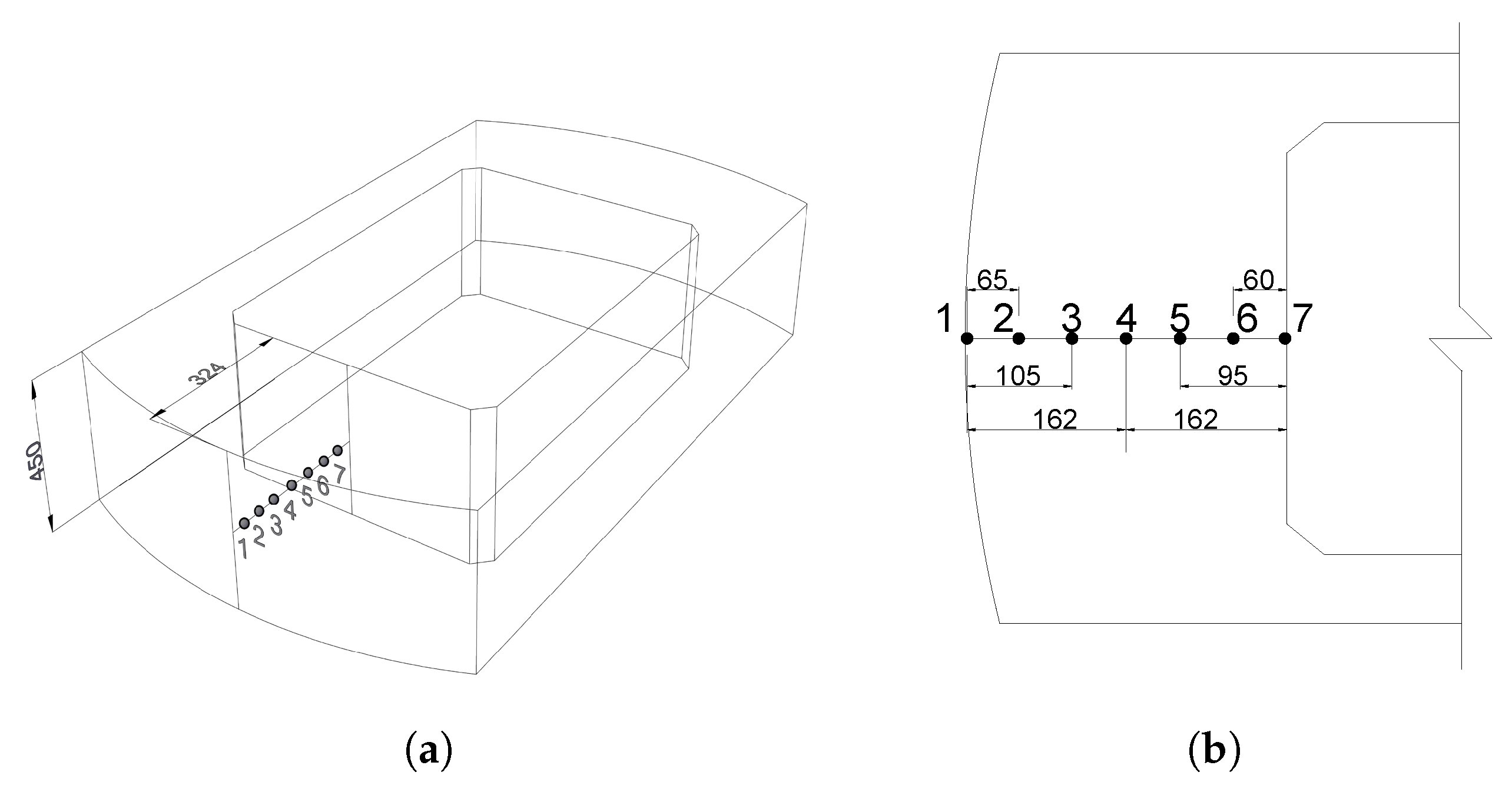
This study was conducted as part of a health monitoring project for a bridge located in Guangxi Province, South China. The main bridge consists of a rigid, frame-continuous girder structure with a span arrangement of $(48+5\times 80+48)$ m (Figure 1). A representative segment (elevation: 22.898–27.398 m) of the box-section rigid frame pier (Pier #4) was selected as the research object (Figure 2). The segment was constructed using C40 concrete with the following mix proportions per cubic meter: a total of 312 kg of Portland cement (Grade 42.5), 750 kg of sand, 1080 kg of coarse aggregate, 125 kg of fly ash, 4.16 kg of superplasticizer, and 154 kg of water. A steel formwork was employed during construction, and the exposed surface was covered with burlap sacks and subjected to water curing after casting.

2.1.2. Data Collection

The dataset collected in this study comprises three components:

(1)

Internal temperature data: Considering the structural symmetry of the pier, seven representative monitoring points were selected for temperature measurement (the distribution is shown in Figure 2). AD592 integrated temperature sensors (Analog Devices, Inc., Wilmington, MA, USA) (measurement range: $-25$ to $105°\mathrm{C}$; accuracy: $\pm 0.1°\mathrm{C}$) were deployed, with data acquisition performed using an LTM8261 handheld tester (Lance Tech, Beijing, China). To capture the rapid hydration heat evolution process, the sampling interval was initially set at 2 h and then adjusted to 4–10 h in later stages, with a total monitoring duration of 450 h.

(2)

Environmental variables: Meteorological data were obtained from a Chinese surface weather station (Station ID: 57957) located approximately 30 km from the construction site. The dataset includes ambient temperature, precipitation, wind speed, humidity, cloud cover, and various components of solar radiation.

(3)

Finite element simulation data: Temperature values at each monitoring point over the same time span were simulated using ANSYS 2024 R1 software through the finite element method, serving as physics-based benchmarks for subsequent comparisons.

2.2. Physics-Based Finite Element Simulation

2.2.1. Governing Equations and Heat Source Model

To establish a conventional first-principles-based benchmark, transient thermal analysis was performed using the commercial finite element software ANSYS Mechanical (2024 R1) [35,36]. A three-dimensional geometric model matching the actual dimensions of the monitored mass concrete structure was created to simulate the temporal evolution of internal temperature. The simulation follows Fourier’s law of heat conduction, with the transient heat diffusion equation serving as both the governing equation and the model for the heat source [37,38].

$$T\left(t\right)=T_{\infty }(1-e^{-a{t}^b})$$

(1)

2.2.2. Model Development and Solution

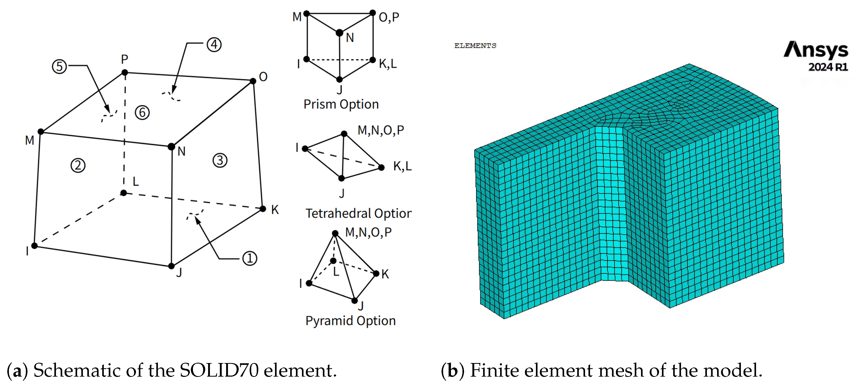
Considering the structural symmetry, a quarter-scale, three-dimensional finite element model was developed. The model employed SOLID70 elements, which are eight-node, three-dimensional isoparametric thermal elements with a single temperature degree of freedom at each node [39,40] (Figure 3a). Following a mesh convergence study, a mesh size of 0.2 m was determined, resulting in a model comprising 9430 elements and 42,618 nodes (Figure 3b). Combined boundary conditions accounting for convection and radiation were applied to the external surfaces, with field-measured ambient temperatures serving as boundary inputs. The specific values of convection coefficients and radiation constants are detailed in

Table 1. Thermal and mechanical properties of the concrete for the FEM model.

Item	Value
Specific heat ($\mathrm{k}\mathrm{J}{\mathrm{kg}}^{-1}°{\mathrm{C}}^{-1}$)	0.98
Density ($\mathrm{k}\mathrm{g}{\mathrm{m}}^{-3}$)	2425
Thermal conductivity ($\mathrm{k}\mathrm{J}{\mathrm{m}}^{-1}{\mathrm{h}}^{-1}°{\mathrm{C}}^{-1}$)	9.32
Convection coefficient (outside) ($\mathrm{k}\mathrm{J}{\mathrm{m}}^{-2}{\mathrm{h}}^{-1}°{\mathrm{C}}^{-1}$)	45
Convection coefficient (inside) ($\mathrm{k}\mathrm{J}{\mathrm{m}}^{-2}{\mathrm{h}}^{-1}°{\mathrm{C}}^{-1}$)	35
Thermal expansion coefficient ($°\mathrm{C}$)	1.0 × 10−5
Poisson’s ratio	0.17
Coefficient of thermal heat source function	$Q_{\infty }=320\mathrm{k}\mathrm{J}{\mathrm{kg}}^{-1}$, $a=0.69$, $b=0.56$

.

2.3. Exploratory Data Analysis: Quantifying Nonlinearity and Time Lag

2.3.1. Nonlinear Relationship Metric: Maximal Information Coefficient (MIC)

To comprehensively evaluate both linear and nonlinear correlations between variables, the Maximal Information Coefficient (MIC) was employed in this study. The MIC assesses association strength by computing the mutual information $I(X;Y)$ between two variables ($X,Y$) and normalizing it [41]. The fundamental approach involves discretizing the two variables in a two-dimensional space and representing them as a scatter plot. This two-dimensional space is partitioned into intervals along both x and y directions, and the dispersion of points within each grid cell is examined to facilitate the calculation of mutual information. The MIC analysis was implemented using the minepy library in Python 3.11.

The constraint $a\times b<B$ is imposed, with B set to approximately 0.6 times the sample size following the original methodology.

$$\mathrm{MIC}(X;Y)=\underset{a\times b<B}{max}{\displaystyle \frac{I(X;Y)}{{log}_2(min(a,b))}}$$

(2)

2.3.2. Analysis Procedure

The analytical workflow was structured as follows: First, a standard Pearson correlation coefficient matrix was generated for the entire dataset to obtain an overall perspective of linear relationships among variables. To further validate the hypothesis of a “two-stage” physical process from a data-driven perspective, the dataset was partitioned into two subsets using the moment when the measured core temperature reached its peak value as the splitting point, creating Stage I (heating stage) and Stage II (cooling stage). Pearson correlation analysis was performed independently on each subset to reveal differences in the dominant driving mechanisms between the two stages. Subsequently, to explore nonlinear relationships, the Maximal Information Coefficient (MIC) was introduced and compared with the Pearson correlation coefficient. Finally, time lag analysis was conducted using MIC by calculating MIC values across different lag steps to determine the optimal time delays for each environmental variable’s influence on core temperature.

2.4. Proposed Two-Stage Hybrid Modeling Strategy

The core insight is that the temperature evolution of mass concrete is not a monolithic process but can be clearly decoupled into two stages governed by different physical mechanisms. The partition point is set at the time when the measured core temperature reaches its peak:

 Stage I: Hydration Heat-Dominated Phase. 

This initial stage is characterized by rapid temperature rise, primarily driven by the deterministic exothermic reaction of cement hydration. The temperature profile exhibits relatively predictable and smooth characteristics [42]. Polynomial regression was employed for this stage to model the relationship between the independent variable (elapsed time since casting) and the dependent variable (temperature) [43]. The general form of the polynomial model is defined as

$$\widehat{T}={\beta }_0+{\beta }_{1}t+{\beta }_2{t}^2+\cdots +{\beta }_n{t}^n$$

(3)

The results of the cross-validation, shown in Figure 4 (left), were used to determine the optimal polynomial order. While the RMSE decreases sharply from order 1 to 2, there is no statistically significant improvement for orders greater than 2, as indicated by the overlapping error bars. Adhering to the principle of parsimony, which favors the simplest model that can explain the data sufficiently, the second-order polynomial ($n=2$) was selected. This choice minimizes the risk of overfitting to the training data and ensures a more generalizable model for the heating stage.

 Stage II: Environment-Dominated Phase. 

After reaching the peak temperature, the concrete enters an extended cooling stage, where evolution is primarily governed by complex, stochastic, and nonlinear interactions with the external environment. To address the complexity of this environment-dominated cooling stage, a Random Forest (RF) regressor was selected for its robustness and capability in handling nonlinear relationships [44,45]. Its fundamental principle is illustrated in Figure 5, where multiple independent decision trees are constructed, and their predictions are aggregated (by averaging in regression tasks) to improve the stability and accuracy of the model. The temperature evolution at this stage is determined by complex, stochastic, and nonlinear interactions with the external environment, making RF an effective choice.

Figure 4. Determination of the optimal polynomial order for the Stage I model via cross-validation and its final fit.

Figure 4. Determination of the optimal polynomial order for the Stage I model via cross-validation and its final fit.

Based on this physical process decoupling, a “two-stage hybrid model” is proposed. The transition point between the two stages is defined as the time step when the measured average core temperature (internal_avg_temp) reaches its maximum value.

2.5. Baseline Models for Comparison

To rigorously evaluate the performance of the hybrid model, four baseline models representing distinct modeling philosophies were selected for comparison. These models were chosen to provide comprehensive benchmarking against the simplest baseline, traditional physics-based simulation, standard end-to-end machine learning approaches, and advanced deep learning methods.

Figure 5. Schematic diagram of the Random Forest regression algorithm.

Figure 5. Schematic diagram of the Random Forest regression algorithm.

2.5.1. Naive Forecast Model

This represents the most fundamental time series baseline model, also known as the persistence model [46]. Its core assumption is that the system state will remain unchanged in the short term [47].

$${\widehat{T}}_t=T_{t-1}$$

(4)

2.5.2. Physics-Based Finite Element Model (FEM)

This model represents the traditional engineering simulation approach based on first principles. As described in Section 2.2, it simulates heat transfer within the structure and heat exchange with the environment by solving the Fourier heat conduction partial differential equation.

In this study, we directly used the nodal temperatures (fem_internal_avg_temp) simulated by ANSYS 2024 R1 software under given initial conditions, boundary conditions, and material properties as the prediction results. This model represents the predictive capability achievable through pure physics-based simulation without calibration using field-measured data.

2.5.3. Single Random Forest Model

This is a powerful end-to-end machine learning model without stage partitioning. Random Forest is an ensemble learning algorithm based on decision trees [48] (Figure 5). It improves prediction accuracy and robustness by constructing numerous decision trees and aggregating their results (typically through averaging for regression problems) [49]. Key techniques include the following:

Bootstrap Aggregating (Bagging).

Multiple sub-training sets are randomly sampled with replacement from the original training set, and each subset is used to train an independent decision tree.

Feature Randomness.

During node splitting in each decision tree, instead of selecting the optimal feature from all available features, the selection is made from a randomly sampled feature subset. This further increases model diversity and effectively prevents overfitting.

In this study, a single Random Forest regressor was employed to directly predict the concrete temperature throughout the entire process. The model’s hyper-parameters were configured as follows: the number of decision trees (n_estimators) was set to 100, a quantity that balances model robustness with computational efficiency. To allow each tree to fully capture the complex, nonlinear relationships within the data, the maximum depth (max_depth) was set to be unrestricted. The mean squared error (criterion=’squared_error’) was used as the splitting criterion, which is a standard choice for regression tasks. To capture fine-grained data features, the minimum number of samples required to split an internal node (min_samples_split) was set to 2, and the minimum number of samples at a leaf node (min_samples_leaf) was set to 1. At each split, the best feature was selected from a random subset, the size of which was the square root of the total number of features (max_features=’sqrt’). This strategy enhances model diversity and effectively mitigates the risk of overfitting.

We trained a single Random Forest regressor using the complete dataset, which contains all environmental and lagged features, to directly predict concrete temperature throughout the entire process. This model aims to examine the performance of a standard, powerful machine learning model without considering physical stage partitioning.

2.5.4. Gated Recurrent Unit (GRU) Model

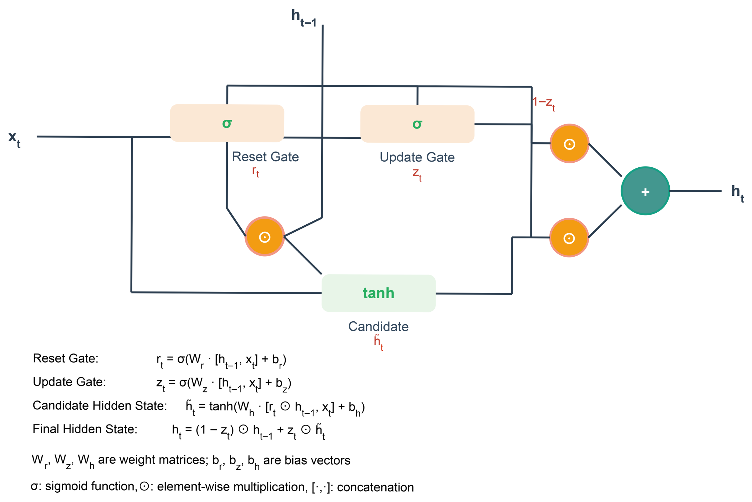
The Gated Recurrent Unit (GRU) network is an advanced recurrent neural network (RNN) specifically designed for processing sequential data [50]. Its internal structure is illustrated in Figure 6, where it effectively captures long-term dependencies in time-series data by introducing two gating mechanisms: the ’update gate’ and the ’reset gate’ [51].

Update Gate ($z_t$).

Determines the extent to which information from the previous time step is carried forward to the current state.

Reset Gate ($r_t$).

Determines how much past information should be ignored when computing the current candidate state.

2.6. Evaluation Metrics

All model performances were quantitatively assessed using three widely accepted standard statistical metrics to ensure comprehensive and objective comparison.

2.6.1. Root Mean Squared Error (RMSE)

RMSE represents the square root of the average of squared differences between predicted and actual values. This metric assigns higher weights to larger errors (outliers), making it highly sensitive to prediction deviations and particularly effective for identifying models with significant prediction failures [52].

$$\mathrm{RMSE}=\sqrt{{\displaystyle \frac{1}{n}}\sum _{i=1}^n{(T_i-{\widehat{T}}_i)}^2}$$

(5)

2.6.2. Mean Absolute Error (MAE)

MAE represents the average of absolute errors for all individual observations. Unlike RMSE, MAE assigns equal weight to all errors, providing a more intuitive reflection of the actual magnitude of prediction errors and demonstrating lower sensitivity to outliers [53].

$$\mathrm{MAE}={\displaystyle \frac{1}{n}}\sum _{i=1}^n|T_i-{\widehat{T}}_i|$$

(6)

2.6.3. Coefficient of Determination ($R^2$)

$R^2$ indicates the degree to which the model explains the variation in the dependent variable. Its value ranges between 0 and 1, where values closer to 1 indicate better model fit to the data, meaning the independent variables can explain a greater proportion of the variation in the dependent variable [54].

$$R^2=1-{\displaystyle \frac{{\sum }_{i=1}^n{(T_i-{\widehat{T}}_i)}^2}{{\sum }_{i=1}^n{(T_i-\overline{T})}^2}}$$

(7)

2.6.4. Evaluation Focus and Cumulative Error Analysis

Although metrics for the entire process were recorded, the primary model evaluation and comparison focused on performance during Stage II (cooling stage). This emphasis reflects the greater complexity and practical importance of accurately predicting temperatures during the environmentally influenced cooling stage.

Beyond these point-wise error metrics, we also plotted cumulative absolute error curves over time for each model during Stage II. This analysis provides crucial insights into the following:

• Long-term model stability: Whether prediction accuracy deteriorates over extended time periods;
• Error accumulation patterns: How individual prediction errors compound over the cooling stage;
• Temporal performance consistency: Model reliability across different time horizons within the cooling stage.

3. Results

3.1. Physical Characteristics and Simulation: Comparative Analysis of Concrete Temperature Fields

3.1.1. Spatiotemporal Evolution Patterns of Measured Temperature Fields

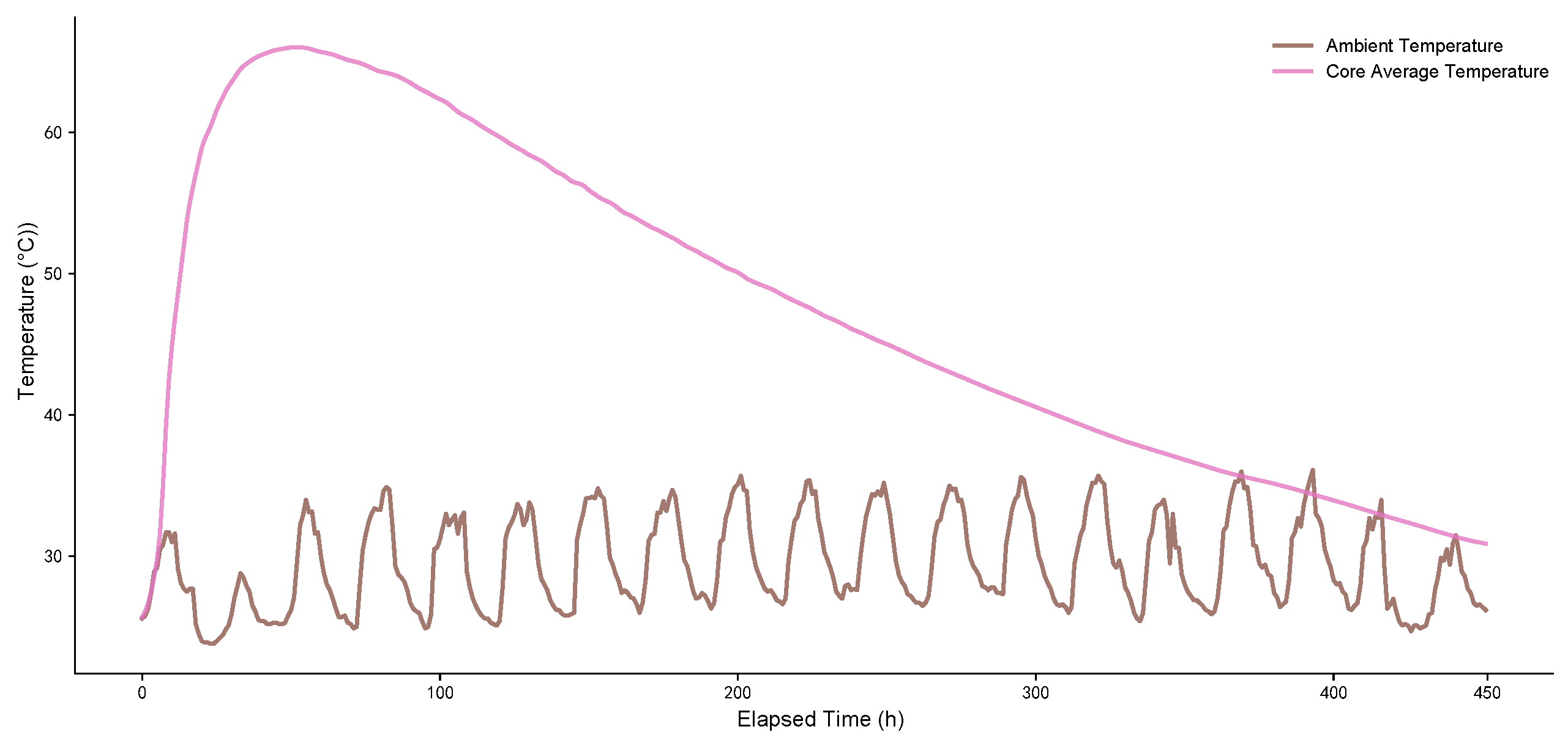
Field monitoring data revealed a unique and complex evolutionary process within the internal temperature fields of mass concrete structures. Figure 7 provides a macroscopic illustration of the temporal relationship between average core temperature and external ambient temperature evolution in concrete. Two fundamental physical phenomena can be clearly observed from the data: First, the concrete core temperature exhibits a distinctive “heating-cooling” two-stage pattern, reaching its peak value at approximately 56 h, which provides intuitive evidence for subsequent stage-decoupled modeling approaches consistent with established hydration kinetics theory in concrete materials science. Second, during the cooling phase, the declining trend of core temperature demonstrates a pronounced correlation with periodic fluctuations in ambient temperature, directly manifesting the coupled interaction between internal and external physical fields, as described in classical heat transfer theory for concrete structures.

To further investigate the details of the internal temperature field, Figure 8 displays the time-history curves of the seven embedded sensors. These curves clearly reveal the following spatiotemporal patterns:

• Spatial Gradient Characteristics: The temperature field exhibits a distinct “onion-like” layered structure. The curves representing the core monitoring points (Points 3 and 4) consistently show the highest recorded temperatures and the strongest heat accumulation effect. In contrast, the curves representing the surface points (Points 1, 6, and 7) are located at the bottom and show greater volatility, indicating their higher sensitivity to environmental changes.
• Temporal Asynchronicity: The temperature evolution at different monitoring points is not synchronous. The curves of the core region reach their peak temperatures last, demonstrating significant thermal inertia and lag. In comparison, the curves of the surface regions respond more rapidly to external environmental conditions.

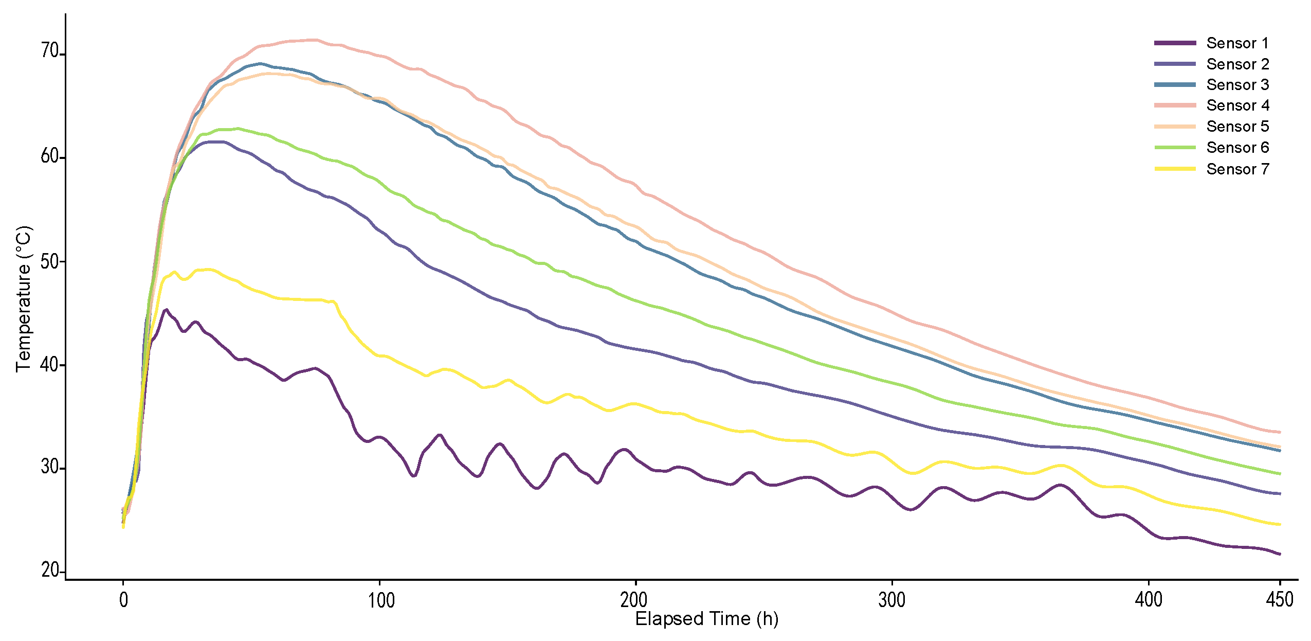
Figure 8. Time-history curves of the temperatures measured by the seven individual sensors.

Figure 8. Time-history curves of the temperatures measured by the seven individual sensors.

3.1.2. Comparative Analysis Between Measured Data and FEM Simulation

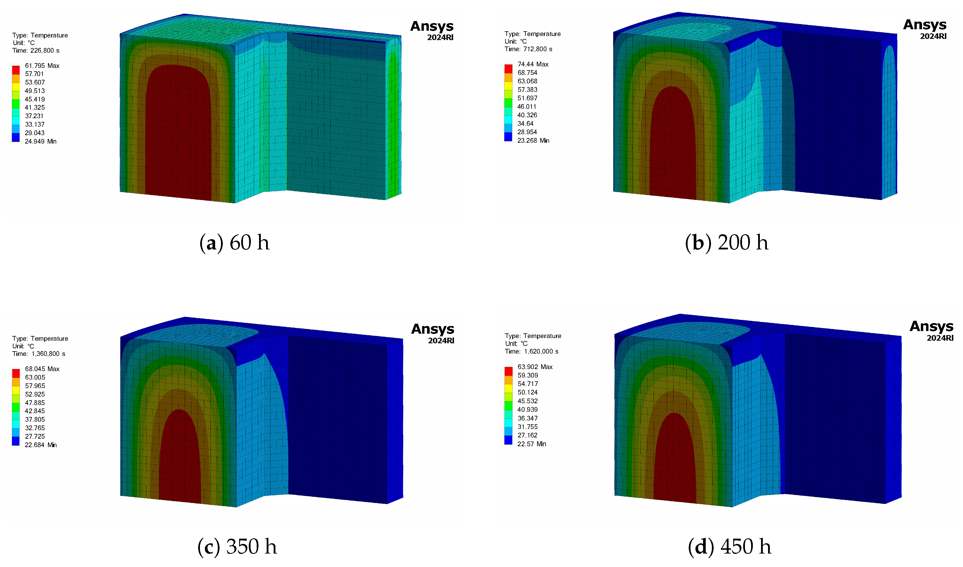
To evaluate the performance of the traditional physical model, we compared the measured data with the FEM simulation results. Figure 9 displays the transient thermal analysis results from the FEM at four key time points (60 h, 200 h, 350 h, and 450 h), which show smooth and regular concentric temperature distributions. The comparison reveals that at the end of the heating stage (Figure 9a, 60 h), the temperature field simulated by the FEM is largely consistent with the measured patterns, both exhibiting internal heat accumulation and a temperature gradient that decreases from the inside out. However, after entering the prolonged cooling stage (Figure 9b–d, discrepancies between the simulated results and the measured data gradually emerge. A quantitative analysis of these stages, shown in Figure 10, reveals a strong correlation between core temperature and time during the initial heating stage (r = 0.89), while this linear correlation vanishes in the cooling stage (r = 0.01), highlighting the model’s inadequacy in this phase. Furthermore, a comparison of different correlation metrics (Figure 11) suggests the presence of complex, potentially non-linear relationships between variables that the deterministic physical model cannot capture The entire cooling process predicted by the FEM (its full time-history curve is shown in Figure 12) is monotonic and smooth. In contrast, the measured data (Figure 7 and Figure 8) exhibit numerous periodic fluctuations, which are likely caused by factors such as diurnal temperature variations. The root of this discrepancy lies in the complexity of physical coupling. While the FEM can effectively simulate the deterministic process dominated by internal hydration heat, its simplified boundary conditions cannot perfectly replicate the instantaneous and dynamic coupling effects between random environmental factors—such as solar radiation, wind, and rain—and the structure’s surface. This gap precisely highlights the inherent limitations of purely physics-based models and provides a compelling justification for introducing a data-driven model in this study [55].

3.2. Quantitative Analysis of Environmental Influences

3.2.1. Correlation Analysis Across Different Physical Phases

To validate the “two-stage” physical process hypothesis from a data-driven perspective, we conducted Pearson correlation analysis on the heating stage (Stage I) and cooling stage (Stage II) data, delineated by the temperature peak point (approximately 48 h). The results are presented in Figure 10, revealing distinctly different driving mechanisms across the two stages.

During Stage I (Figure 10a), the core temperature exhibits an extremely strong positive correlation with elapsed time ($r=0.89$) while demonstrating relatively weak correlations with all environmental variables that are consistent with the internal heat generation processes documented in concrete hydration studies. This provides compelling evidence that this stage represents a relatively independent, deterministic process dominated by internal hydration heat release following established principles of concrete thermal behavior during early-age development.

In Stage II (Figure 10b), the linear correlation between core temperature and environmental temperature (env_temp) approaches nearly zero ($r=0.01$). This unexpected result presents a striking contrast to the macroscopic associations observed in Figure 7, strongly suggesting the existence of more complex, nonlinear, or time-delayed relationships between these variables, which reflects the sophisticated nature of environmental coupling in concrete thermal systems. This phase-based correlation comparison provides decisive data evidence supporting the necessity of decoupling physical processes and seeking more powerful nonlinear analytical tools and modeling methodologies for the second stage, aligning with advanced approaches in concrete thermal modeling research.

Figure 10. Comparison of Pearson correlation coefficients for the two distinct physical stages. (a) Stage I (Heating Stage, <48 h), where the core temperature is strongly correlated with elapsed time (r = 0.89). (b) Stage II (Cooling Stage, >48 h), where the linear correlation between core temperature and ambient temperature is nearly zero (r = 0.01).

Figure 10. Comparison of Pearson correlation coefficients for the two distinct physical stages. (a) Stage I (Heating Stage, <48 h), where the core temperature is strongly correlated with elapsed time (r = 0.89). (b) Stage II (Cooling Stage, >48 h), where the linear correlation between core temperature and ambient temperature is nearly zero (r = 0.01).

3.2.2. Nonlinear and Time-Lag Analysis

To further investigate the complex, nonlinear dependencies present in Stage II, we implemented the Maximal Information Coefficient (MIC) for comparative analysis following established principles of nonlinear correlation detection in complex systems. As illustrated in Figure 11, numerous variable pairs exhibit MIC values (y-axis) that significantly exceed the absolute values of their Pearson correlation coefficients (x-axis), with these data points markedly deviating from the $y=x$ diagonal line. This provides clear quantitative evidence for the existence of strong nonlinear coupling interactions within the system, explaining why simple linear models prove insufficient for describing the behavior of the complete system.

Furthermore, considering the thermal inertia inherent in mass concrete structures, their response to environmental changes is not instantaneous, which is consistent with the thermal diffusivity characteristics established in research on concrete materials. We employed MIC analysis to conduct time-lag investigations to determine the optimal timing for the influence of various meteorological factors. As presented in

Table 2. Table of MIC values at different time steps.

Variable	Step 0	Step 1	Step 2	Step 3	Step 4	Step 5	Best Lag (hours)	Max MIC Value
env_temp	0.472	0.477	0.488	0.489	0.476	0.483	3	0.489
precipitation	0.209	0.211	0.213	0.219	0.224	0.217	4	0.224
wind_speed	0.281	0.271	0.272	0.265	0.273	0.270	0	0.281
humidity	0.468	0.484	0.487	0.476	0.452	0.465	2	0.487
cloud_cover	0.535	0.526	0.534	0.529	0.529	0.542	5	0.542

, different environmental factors demonstrate varying delay effects on core temperature evolution.

For instance, the effect of wind speed is instantaneous (0-h lag). In contrast, the influence of cloud cover has a lag of up to 5 h and possesses the highest MIC value among all factors (0.542), indicating its profound impact. In summary, the quantitative analysis of environmental impacts demonstrates that the concrete-cooling process is governed by a complex physical coupling involving multiple variables, strong nonlinearity, and time lags. This conclusion provides a solid data-theoretic basis for subsequently employing a machine learning model, such as Random Forest, capable of capturing these characteristics to specifically model the second stage.

Figure 11. Comparison of the Maximal Information Coefficient (MIC) and the absolute Pearson correlation coefficient for all variable pairs.

Figure 11. Comparison of the Maximal Information Coefficient (MIC) and the absolute Pearson correlation coefficient for all variable pairs.

3.3. Comparative Analysis of Model Performance

3.3.1. Quantitative Performance Evaluation

To definitively assess the effectiveness of different modeling strategies, we conducted comprehensive performance comparisons between our proposed two-stage hybrid model and four benchmark models. The evaluation focus was placed on the cooling stage (Stage II), which holds the most engineering significance for temperature crack control, consistent with established practices in concrete thermal management evaluation.

Table 3. Comparison of different model performance metrics.

Model	RMSE $(°\mathrm{C})$	MAE $(°\mathrm{C})$	R2 Score
Hybrid Model	0.24	0.18	0.995
Random Forest	0.29	0.20	0.993
Naive Forecast	0.35	0.25	0.990
GRU Model	0.81	0.67	0.945
Pure FEM Model	1.55	1.39	0.813

summarizes the data, showing that our proposed hybrid model performed optimally across all metrics, achieving the lowest Root Mean Squared Error (RMSE = 0.24 °C). Compared to the second-best performing single Random Forest model (RMSE = 0.29 °C), the hybrid model’s error was reduced by 17.2%, indicating a significant performance improvement. In contrast, the prediction accuracy of the traditional physics-based FEM model and the advanced GRU deep learning model was far from satisfactory in this complex scenario. Notably, although the single Random Forest model (Single RF) ranks second in performance, its errors remain significantly higher than those of the hybrid model, demonstrating the value of the physics-informed model architecture design principles documented in the hybrid modeling literature [56]. The traditional pure physics FEM model and advanced GRU deep learning model exhibit far-from-satisfactory prediction accuracy in this complex scenario, highlighting the challenges faced by single-approach methodologies in complex thermal systems, as recognized in computational modeling research.

3.3.2. Visual Performance Analysis and Detail Capture

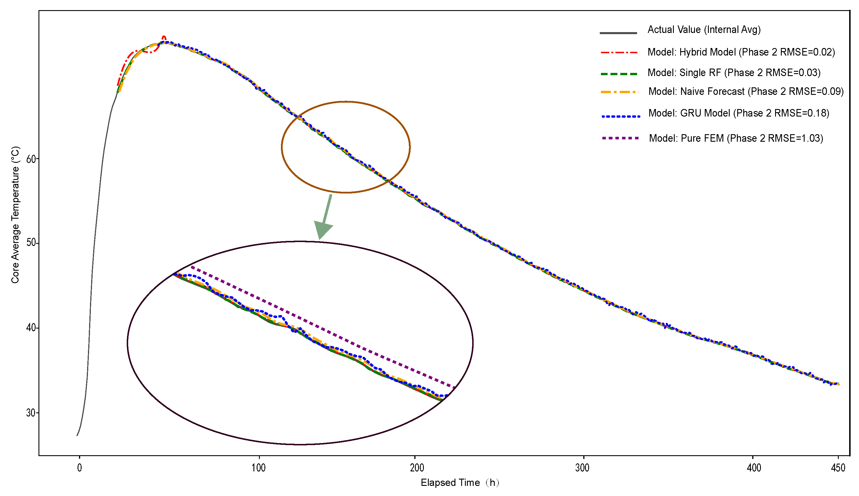
Figure 12 provides an intuitive comparison of prediction curves from various models against actual values. Macroscopically, all data-driven models can approximately capture the overall cooling trend consistent with the general capability of machine learning approaches in time series modeling applications. However, the embedded local magnification inset (picture-in-picture) reveals substantial differences in the models’ detail-capture capabilities. Within a critical region where environmental fluctuations induce significant temperature variations, the hybrid model’s prediction curve (red dashed line) closely follows the subtle undulations of actual temperature values, demonstrating a strong ability to capture complex environmental coupling effects, as desired in advanced concrete thermal modeling. In contrast, all other models, including the second-best-performing single Random Forest model, exhibit prediction curves that appear overly smooth or contain obvious deviations, failing to accurately reflect the true physical processes and highlighting their limitations.

Figure 12. Comparison of the predicted temperature curves from different models.

Figure 12. Comparison of the predicted temperature curves from different models.

3.3.3. Long-Term Stability and Reliability Assessment

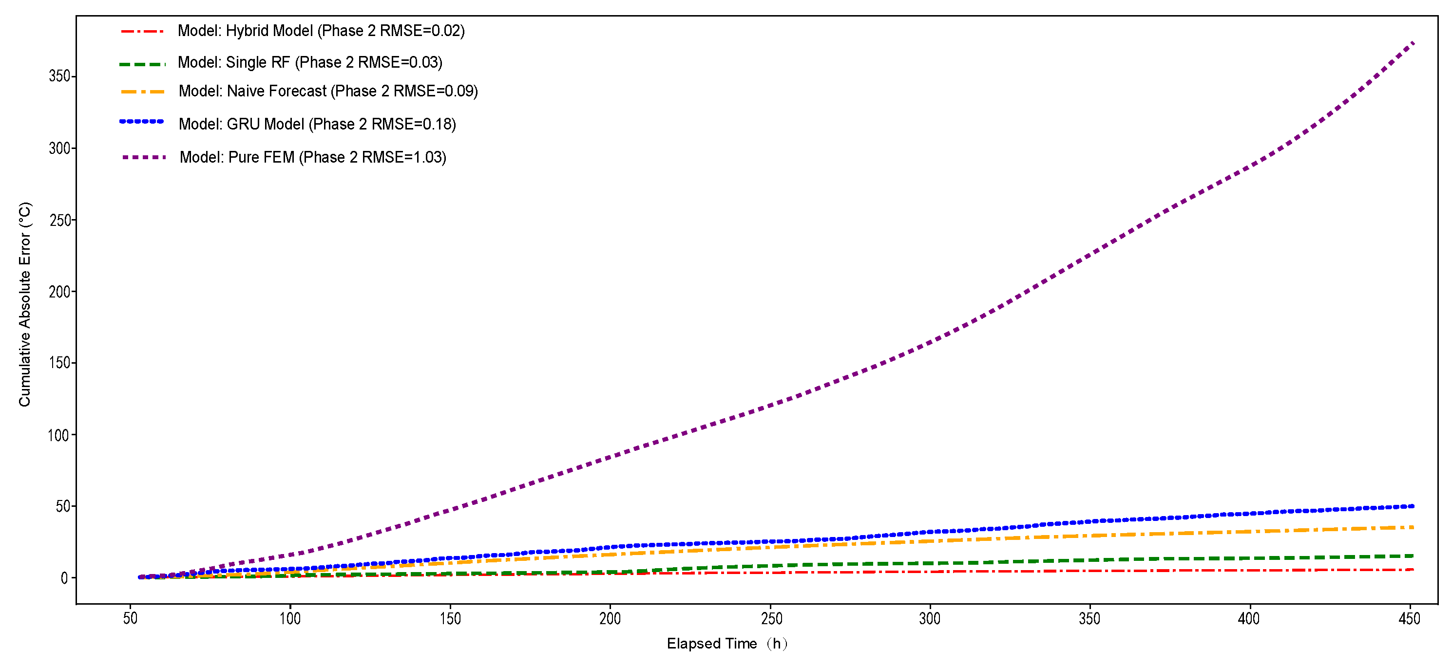
To further evaluate the long-term stability and reliability of the models, we plotted cumulative absolute error curves for each model during Stage II (Figure 13). This analysis provides quantitative evidence regarding the comparative performance of the models in maintaining long-term prediction accuracy.

As shown in Figure 13, the hybrid model’s cumulative error curve (red dashed line) exhibits the gentlest slope. At the end of the 450-h monitoring period, its final cumulative absolute error was approximately 5 °C. This is substantially lower than that of its direct competitors, the Single RF model (approximately 15 °C) and the GRU model (approximately 50 °C). The Pure FEM model showed the most rapid error accumulation, reaching a final cumulative error of over 350 °C. This result is particularly noteworthy: while the single Random Forest model demonstrates relatively low point-wise errors (RMSE = 0.03 °C), its cumulative error is approximately three times that of the hybrid model (RMSE = 0.02 °C). This highlights the tendency for error to accumulate in single-stage models, impacting their long-term prediction reliability—a finding that is consistent with the documented limitations of monolithic models in sustained prediction tasks [57].

4. Discussion

This research aims to investigate whether a “two-stage hybrid modeling” strategy based on physical process decoupling can provide more accurate and reliable predictions of early-age temperature evolution in mass concrete structures compared to traditional single-model approaches. The results suggest that this strategy shows promise, particularly during the cooling stage, which holds significant importance for engineering practice. This section explores the underlying physical mechanisms and model behaviors that contribute to these observations.

4.1. Potential Sources of Hybrid Model Performance: Physics-Informed Design

The encouraging performance of the hybrid model stems from a design philosophy that aligns its architecture with the intrinsic physical mechanisms of concrete temperature evolution. Our exploratory data analysis (Section 3.2.1) provides data-driven evidence supporting the validity of the “two-stage” hypothesis:

During Stage I (heating stage), the temperature evolution is dominated by the internal, exothermic chemical reaction of cement hydration. In these early hours, the rate of internal heat generation far surpasses the rate of heat exchange with the ambient environment. This internal dominance physically explains the observed strong positive correlation with time ($r=0.89$) and the relative insensitivity to external weather fluctuations. The process follows a predictable, chemistry-driven trajectory that is both relatively independent and deterministic. Consequently, employing a parsimonious polynomial regression model is not merely computationally efficient but physically appropriate, as its mathematical form effectively captures the smooth, monotonic nature of this internally governed heating process.

During Stage II (cooling stage), a critical shift in the governing physics occurs. As the hydration reaction rate slows, the dominant mechanism transitions from internal heat generation to the complex heat exchange at the concrete’s surface [58]. This process is governed by a simultaneous and intricate interplay of convection (driven by wind and temperature gradients), radiation (solar gains and longwave emission), and evaporation (moisture removal influenced by humidity and wind). These heat transfer modes are inherently nonlinear and coupled; for instance, strong solar radiation may increase temperature, while concurrent high wind speeds enhance convective and evaporative cooling. This dynamic and often competing interaction among multiple environmental variables explains why a simple linear correlation between core and environmental temperature is negligible ($r=0.01$) and why advanced analysis reveals strong nonlinearities. Therefore, the selection of a Random Forest model for this stage is a direct response to this physical complexity. Its ability to capture high-dimensional, nonlinear interactions without a predefined physical equation makes it uniquely suited for this data-rich, mechanistically complex stage.

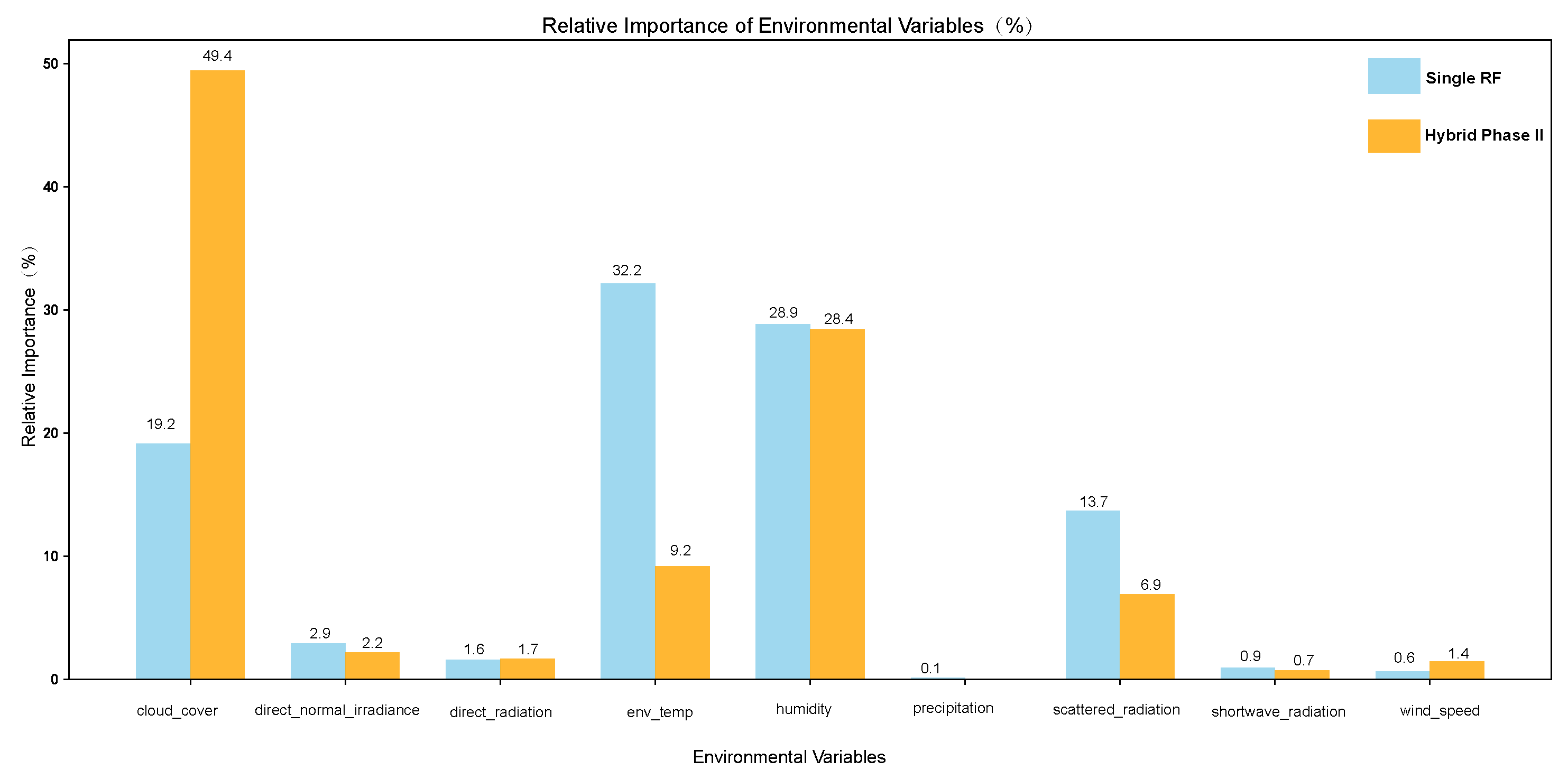
To provide data-driven validation for this approach, we conducted a comparative feature importance analysis, examining how the Single RF model and our hybrid model’s second stage prioritize environmental variables. As demonstrated in Figure 14, the hybrid model correctly identifies cloud cover—a key factor governing longwave radiative cooling—as the most critical environmental variable, assigning it 49.4% of the relative importance within the environmental feature set. In stark contrast, the Single RF model significantly underestimates its role, prioritizing ambient temperature (32.2%) and humidity (28.9%) instead. This provides compelling evidence that by decoupling the physical processes, our hybrid approach is significantly more effective at identifying the true, stage-specific physical drivers—a feat that the end-to-end model fails to achieve.

4.2. Analysis of Individual Model Limitations

The performance of benchmark models in this study, particularly the seemingly competitive results of the single Random Forest (Single RF) model, provides valuable insights into modeling challenges, highlighting important considerations for complex-system-modeling approaches.

• Single Random Forest model considerations: Although the Single RF model performed acceptably in terms of point-wise errors (RMSE and MAE), its cumulative absolute error curve (Figure 13) reveals a critical shortcoming. For engineering problems driven by extreme values and persistent deviations, such as thermal cracking, systematic bias is far more detrimental than random error.
• FEM and GRU model performance: The limitations of the traditional FEM model stem mainly from its simplified boundary conditions. Our correlation analysis (Figure 10) has demonstrated that the real environment is a complex system with highly inter-correlated factors (temperature, humidity, radiation, etc.). This dynamic coupling is difficult to describe accurately with a few fixed heat transfer coefficients. The suboptimal performance of the advanced GRU model highlights the issue of data efficiency. Without being endowed with prior knowledge of the physical stage transition, a deep learning model would require a much larger dataset than the one used in this study to learn the implicit transition patterns on its own. This demonstrates that our hybrid model achieves higher efficiency and accuracy on small to medium-sized datasets by incorporating physical insights.

4.3. Contributions and Broader Impact

This research contributes to the broader field of engineering system modeling beyond concrete temperature prediction. The proposed “physics-informed hybrid modeling through process decoupling” framework may offer insights for addressing other complex engineering problems characterized by multi-stage behavior, such as material curing processes, soil consolidation, and battery charge–discharge cycles, extending the applicability of hybrid modeling principles to related engineering domains.

While studies such as those by Huang et al. [59] utilize machine learning for predicting material properties from static components, our research focuses on the dynamic evolution of materials under time-varying environmental conditions. These two lines of inquiry are complementary; they address distinct aspects of machine learning applications in civil engineering materials: ’static component-property’ relationships and ’dynamic environment-response’ interactions. This work thereby expands the existing research on data-driven approaches by addressing the latter dimension.

4.4. Limitations and Future Work

The authors acknowledge several limitations in the present study that offer important avenues for future research.

First and foremost, the validation of the proposed hybrid framework was conducted using a single, full-scale dataset from a specific bridge project in a subtropical climate, with a single C40 concrete mixture, which represents the most significant limitation of our study. While the model demonstrated high accuracy and stable performance in this specific case, its generalizability and robustness across a wider range of conditions have not yet been established. Future work must focus on cross-validating the model on multiple, heterogeneous datasets to rigorously assess its performance under diverse conditions, including the following:

• Varying climatic environments, especially cold climates;
• Different concrete mix designs, such as those with high supplementary cementitious material (SCM) content;
• Diverse structural geometries and volumes.

Secondly, the meteorological data used as input was sourced from a weather station located 30 km from the construction site. This distance means the data may not perfectly represent the on-site microclimate. A valuable next step would be to conduct a sensitivity analysis to formally check the model’s robustness to potentially noisy or less representative input data.

Finally, the current stage division method relies on the identification of the temperature peak, which introduces a dependency on the specific data characteristics. Future research could explore more automated and robust phase transition detection methods to enhance the approach’s applicability and reduce the manual oversight required.

By addressing these limitations, future research can build upon our proposed two-stage framework to develop a more generalizable and reliable tool for predicting concrete temperature.

5. Conclusions

This study addressed the challenge of multi-stage physical characteristics (“hydration-dominated” vs. “environment-dominated”) in the early-age temperature prediction of mass concrete by proposing and validating a novel “two-stage hybrid modeling” strategy. The main conclusions are as follows:

• Through a stage-wise correlation analysis of the on-site monitoring data, this study confirmed that, from a data-driven perspective, the heating and cooling stages of concrete are governed by distinctly different physical mechanisms, providing a solid theoretical basis for the process-decoupling modeling approach.
• In the cooling stage, which is crucial for engineering crack control, the proposed two-stage hybrid model significantly outperformed traditional finite element models, single end-to-end machine learning models, and the advanced deep learning GRU model in terms of both prediction accuracy $(\mathrm{RMSE}=0.24°\mathrm{C})$ and the ability to capture details of actual temperature fluctuations.
• The cumulative absolute error analysis proved that the hybrid model exhibits the best long-term prediction stability, with a significantly lower error accumulation rate compared to other models. This highlights the risk that blindly adopting a purely data-driven model may result in insufficient reliability in long-term predictions.

References

1. Zhang, Y.; Kim, T.; Castel, A.; Xu, T. Thermal Cracking in High Volume of Fly Ash and GGBFS Concrete. Int. J. Concr. Struct. Mater. 2023, 17, 65. [Google Scholar] [CrossRef]
2. Smolana, A.; Klemczak, B.; Azenha, M.; Schlicke, D. Thermo-Mechanical Analysis of Mass Concrete Foundation Slabs at Early Age—Essential Aspects and Experiences from the FE Modelling. Materials 2022, 15, 1815. [Google Scholar] [CrossRef] [PubMed]
3. Tyurina, V.; Chepurnenko, A.; Akopyan, V. Prediction of Thermal Cracking during Construction of Massive Monolithic Structures. Appl. Sci. 2025, 15, 1499. [Google Scholar] [CrossRef]
4. Zhang, J.; Zhou, D.; He, X.; Hu, X.; Qiang, S. Comparative Analysis of Temperature and Stress Simulations in Mass Concrete for Sluice Gate Structures Based on Chinese and American Standards. Materials 2025, 18, 100. [Google Scholar] [CrossRef] [PubMed]
5. Zhang, S.; Liu, P.; Liu, L.; Huang, J.; Cheng, X.; Chen, Y.; Chen, L.; He, S.; Zhang, N.; Yu, Z. Heat of Hydration Analysis and Temperature Field Distribution Study for Super-Long Mass Concrete. Coatings 2024, 14, 369. [Google Scholar] [CrossRef]
6. Rahman, M.A.; Zhang, T.; Lu, Y. PINN-CHK: Physics-informed Neural Network for High-Fidelity Prediction of Early-Age Cement Hydration Kinetics. Neural Comput. Appl. 2024, 36, 13665–13687. [Google Scholar] [CrossRef]
7. Klemczak, B.; Smolana, A. Multi-Step Procedure for Predicting Early-Age Thermal Cracking Risk in Mass Concrete Structures. Materials 2024, 17, 3700. [Google Scholar] [CrossRef]
8. Do, T.A.; Le, B.A. Machine Learning Approach for Predicting Early-Age Thermal Cracking Potential in Concrete Bridge Piers. Forces Mech. 2024, 17, 100297. [Google Scholar] [CrossRef]
9. Zhang, M.; Yao, X.; Guan, J.; Li, L. Study on Temperature Field Massive Concrete in Early Age Based on Temperature Influence Factor. Adv. Civ. Eng. 2020, 2020, 8878974. [Google Scholar] [CrossRef]
10. Jeong, D.; Kim, T.; Ryu, J.; Kim, J.H. Analytical model to parameterize the adiabatic temperature rise of concrete. Constr. Build. Mater. 2021, 268, 121656. [Google Scholar] [CrossRef]
11. An, G.; Yang, N.; Li, Q.; Hu, Y.; Yang, H. A Simplified Method for Real-Time Prediction of Temperature in Mass Concrete at Early Age. Appl. Sci. 2020, 10, 4451. [Google Scholar] [CrossRef]
12. Ju, Y.; Lei, H. Actual Temperature Evolution of Thick Raft Concrete Foundations and Cracking Risk Analysis. Adv. Mater. Sci. Eng. 2019, 2019, 7029671. [Google Scholar] [CrossRef]
13. Bui, A.K.; Nguyen, T.C. The Temperature Field in Mass Concrete with Different Placing Temperatures. Civ. Eng. Archit. 2020, 8, 94–100. [Google Scholar] [CrossRef]
14. Jin, C.; Zou, F.; Meng, H.; Jianguo, M.; Zhou, C. A comparative study of temperature of mass concrete placed in August and November based on on-site measurement. Case Stud. Constr. Mater. 2021, 15, e00694. [Google Scholar] [CrossRef]
15. Sargam, Y.; Faytarouni, M.; Riding, K.; Wang, K.; Jahren, C.; Shen, J. Predicting thermal performance of a mass concrete foundation—A field monitoring case study. Case Stud. Constr. Mater. 2019, 11, e00289. [Google Scholar] [CrossRef]
16. Pandhare, S. Temperature Behavior of Mass Concrete in Stage Pre, during and Post: Review. Int. J. Res. Appl. Sci. Eng. Technol. 2020, 8, 1941–1944. [Google Scholar] [CrossRef]
17. Rajaee, T.; Khani, S.; Ravansalar, M. Artificial intelligence-based single and hybrid models for prediction of water quality in rivers: A review. Chemom. Intell. Lab. Syst. 2020, 200, 103978. [Google Scholar] [CrossRef]
18. Gong, L.; Wang, C. Model of Automobile Parts Sale Prediction Based on Nonlinear Periodic Gray GM(1,1) and Empirical Research. Math. Probl. Eng. 2019, 2019, 3620120. [Google Scholar] [CrossRef]
19. Cao, L.; Li, Y.; Zhang, J.; Jiang, Y.; Han, Y.; Wei, J. Electrical load prediction of healthcare buildings through single and ensemble learning. Energy Rep. 2020, 6, 2751–2767. [Google Scholar] [CrossRef]
20. Gao, Y.; Han, J.; Ma, P.; Ji, H.; Zhao, C. Finite Element Method-Based Temperature Field Analysis of Early Age Frozen Shaft Lining with Temperature-Dependent Characteristics. J. Eng. Sci. Technol. Rev. 2022, 15, 89–96. [Google Scholar] [CrossRef]
21. Han, Y.; Zhang, L.; He, J. Influence of Structural Form on Hydration-Heat-Induced Temperature Rise of Precast Concrete Lining Segments for a Metro Transit Station. PCI J. 2023, 68, 88–100. [Google Scholar] [CrossRef]
22. Pham, D.P.; Nguyen, T.C.; Vu, K.D. The Effect of Thermo-Mechanical Properties of Concrete on the Temperature Field in Mass Concrete. Eng. Technol. Appl. Sci. Res. 2024, 14, 17209–17213. [Google Scholar] [CrossRef]
23. Sun, Q.; Ding, B.; Zheng, Z.; Du, R.; Qiang, S. Study on Temperature Control and Crack Prevention of Mass Concrete for Large Powerhouse Constructed in Cold Area. MATEC Web Conf. 2019, 275, 2009. [Google Scholar] [CrossRef]
24. Ahorro, J.R.F.; Estores, G.B. Prediction of Cracking Probability in Mass Concrete Due to High Temperature Using Monte Carlo Simulation. Civ. Eng. Archit. 2024, 12, 2303–2325. [Google Scholar] [CrossRef]
25. Wang, X.; Li, H.; He, L.; Li, Z. Evaluation of multi-objective inverse heat conduction problem based on particle swarm optimization algorithm, normal distribution and finite element method. Int. J. Heat Mass Transf. 2018, 127, 1114–1127. [Google Scholar] [CrossRef]
26. Tian, H.; Liu, Z.; Jia, Y.; Shao, Y. Finite Element Method Parameter Estimation of Atomic Sensor Based on Thermal Network Method. IEEE Sens. J. 2021, 21, 18887–18896. [Google Scholar] [CrossRef]
27. Gajek, S.; Schneider, M.; Böhlke, T. An FE-DMN method for the multiscale analysis of thermomechanical composites. Comput. Mech. 2021, 69, 1087–1113. [Google Scholar] [CrossRef]
28. Abdel-Raheem, M.; Quintana, O.; Morales, M.; Marroquin-Villa, Y.; Ramos, D.; Hernandez, S. Construction Methods Used for Controlling Temperature in Mass Concrete Structure. In Proceedings of the Creative Construction Conference 2018—Proceedings, Ljubljana, Slovenia, 30 June–3 July 2018; Budapest University of Technology and Economics: Budapest, Hungary, 2018; pp. 139–146. [Google Scholar] [CrossRef]
29. Lapeyre, J.; Han, T.; Wiles, B.; Ma, H.; Huang, J.; Sant, G.; Kumar, A. Machine Learning Enables Prompt Prediction of Hydration Kinetics of Multicomponent Cementitious Systems. Sci. Rep. 2021, 11, 3922. [Google Scholar] [CrossRef] [PubMed]
30. Lu, L.; Li, Y.; Wang, Y.; Wang, F.; Lu, Z.; Liu, Z.; Jiang, J. Prediction of Hydration Heat for Diverse Cementitious Composites through a Machine Learning-Based Approach. Materials 2024, 17, 715. [Google Scholar] [CrossRef]
31. Cook, R.; Han, T.; Childers, A.; Ryckman, C.; Khayat, K.; Ma, H.; Huang, J.; Kumar, A. Machine Learning for High-Fidelity Prediction of Cement Hydration Kinetics in Blended Systems. Mater. Des. 2021, 208, 109920. [Google Scholar] [CrossRef]
32. Liu, D.; Zhang, W.; Tang, Y.; Jian, Y. Prediction of Hydration Heat of Mass Concrete Based on the SVR Model. IEEE Access 2021, 9, 62935–62945. [Google Scholar] [CrossRef]
33. Wan, Y.; Zheng, W.; Wang, Y. Identification of chloride diffusion coefficient in concrete using physics-informed neural networks. Constr. Build. Mater. 2023, 393, 132049. [Google Scholar] [CrossRef]
34. Elkhadrawi, M.; Ng, C.; Bain, D.J.; Sargent, E.E.; Stearsman, E.V.; Gray, K.A.; Akcakaya, M. Novel physics informed-neural networks for estimation of hydraulic conductivity of green infrastructure as a performance metric by solving Richards–Richardson PDE. Neural Comput. Appl. 2024, 36, 5555–5569. [Google Scholar] [CrossRef]
35. Castilho, E.; Schclar, N.; Tiago, C.; Farinha, M.L.B. FEA model for the simulation of the hydration process and temperature evolution during the concreting of an arch dam. Eng. Struct. 2018, 173, 805–817. [Google Scholar] [CrossRef]
36. Cucinotta, F.; D’Aveni, A.; Guglielmino, E.; Risitano, A.; Risitano, G.; Santonocito, D. Thermal Emission analysis to predict damage in specimens of High Strength Concrete. Frat. Integrità Strutt. 2020, 15, 233–241. [Google Scholar] [CrossRef]
37. Torelli, G.; Gillie, M.; Mandal, P.; Draup, J.; Tran, V. A moisture-dependent thermomechanical constitutive model for concrete subjected to transient high temperatures. Eng. Struct. 2020, 210, 110170. [Google Scholar] [CrossRef]
38. Asadi, I.; Shafigh, P.; Hassan, Z.; Mahyuddin, N. Thermal conductivity of concrete—A review. J. Build. Eng. 2018, 20, 81–93. [Google Scholar] [CrossRef]
39. Vizzaccaro, A.; Givois, A.; Longobardi, P.; Shen, Y.; Deü, J.; Salles, L.; Touzé, C.; Thomas, O. Non-intrusive reduced order modelling for the dynamics of geometrically nonlinear flat structures using three-dimensional finite elements. Comput. Mech. 2020, 66, 1293–1319. [Google Scholar] [CrossRef]
40. Şorohan, Ş.; Constantinescu, D.; Sandu, M.; Sandu, A. Using point symmetry in finite element analyses. Mater. Today Proc. 2020, 32, 139–147. [Google Scholar] [CrossRef]
41. Liang, T.; Zhang, Q.; Hong, L.; Liu, X.; Dong, B.; Wang, H.; Liu, X. An improved maximal information coefficient algorithm applied in the analysis of functional corticomuscular coupling for stroke patients. Sheng Xue Gong Cheng Xue Zhi J. Biomed. Eng. Shengwu Yixue Gongchengxue Zazhi 2021, 38 6, 1154–1162. [Google Scholar] [CrossRef]
42. Liu, C.; Zhao, C.; Wang, Y.; Wang, H. Machine-Learning-Based Calibration of Temperature Sensors. Sensors 2023, 23, 7347. [Google Scholar] [CrossRef]
43. Nandi, A. Model Order Selection from Noisy Polynomial Data Without Using Any Polynomial Coefficients. IEEE Access 2020, 8, 130417–130430. [Google Scholar] [CrossRef]
44. Amin, M.; Khan, K.; Ahmad, W.; Javed, M.; Qureshi, H.; Saleem, M.U.; Qadir, M.G.; Faraz, M.I. Compressive Strength Estimation of Geopolymer Composites through Novel Computational Approaches. Polymers 2022, 14, 2128. [Google Scholar] [CrossRef]
45. Dai, B.; Gu, C.; Zhao, E.; Qin, X. Statistical model optimized random forest regression model for concrete dam deformation monitoring. Struct. Control Health Monit. 2018, 25, e2170. [Google Scholar] [CrossRef]
46. Sahoo, B.B.; Jha, R.; Singh, A.; Kumar, D. Long short-term memory (LSTM) recurrent neural network for low-flow hydrological time series forecasting. Acta Geophys. 2019, 67, 1471–1481. [Google Scholar] [CrossRef]
47. Janke, T.; Steinke, F. Forecasting the Price Distribution of Continuous Intraday Electricity Trading. Energies 2019, 12, 4262. [Google Scholar] [CrossRef]
48. Karabadji, N.E.I.; Korba, A.A.; Assi, A.; Seridi-Bouchelaghem, H.; Aridhi, S.; Dhifli, W. Accuracy and diversity-aware multi-objective approach for random forest construction. Expert Syst. Appl. 2023, 225, 120138. [Google Scholar] [CrossRef]
49. Cheng, L.; Chen, X.; Vos, J.D.; Lai, X.; Witlox, F. Applying a random forest method approach to model travel mode choice behavior. Travel Behav. Soc. 2019, 14, 1–10. [Google Scholar] [CrossRef]
50. Shu, W.; Cai, K.; Xiong, N. A Short-Term Traffic Flow Prediction Model Based on an Improved Gate Recurrent Unit Neural Network. IEEE Trans. Intell. Transp. Syst. 2021, 23, 16654–16665. [Google Scholar] [CrossRef]
51. Wang, Y.; Liao, W.; Chang, Y. Gated Recurrent Unit Network-Based Short-Term Photovoltaic Forecasting. Energies 2018, 11, 2163. [Google Scholar] [CrossRef]
52. Chakraborty, D.; Elzarka, H. Performance testing of energy models: Are we using the right statistical metrics? J. Build. Perform. Simul. 2018, 11, 433–448. [Google Scholar] [CrossRef]
53. Wang, W.; Lu, Y. Analysis of the Mean Absolute Error (MAE) and the Root Mean Square Error (RMSE) in Assessing Rounding Model. IOP Conf. Ser. Mater. Sci. Eng. 2018, 324, 012049. [Google Scholar] [CrossRef]
54. Shi, X.; Jiang, D.; Qian, W.; Liang, Y. Application of the Gaussian Process Regression Method Based on a Combined Kernel Function in Engine Performance Prediction. ACS Omega 2022, 7, 41732–41743. [Google Scholar] [CrossRef] [PubMed]
55. Hocine, S.; Swygenhoven, H.; Petegem, S. Verification of selective laser melting heat source models with operando X-ray diffraction data. Addit. Manuf. 2021, 37, 101747. [Google Scholar] [CrossRef]
56. Shlezinger, N.; Whang, J.; Eldar, Y.C.; Dimakis, A. Model-Based Deep Learning. Proc. IEEE 2020, 111, 465–499. [Google Scholar] [CrossRef]
57. Pham, B.; Qi, C.; Ho, L.S.; Nguyen-Thoi, T.; Al-Ansari, N.; Nguyen, M.D.; Nguyen, H.; Ly, H.; Le, H.V.; Prakash, I. A Novel Hybrid Soft Computing Model Using Random Forest and Particle Swarm Optimization for Estimation of Undrained Shear Strength of Soil. Sustainability 2020, 12, 2218. [Google Scholar] [CrossRef]
58. Kwon, B.; Ejaz, F.; Hwang, L. Machine learning for heat transfer correlations. Int. Commun. Heat Mass Transf. 2020, 116, 104694. [Google Scholar] [CrossRef]
59. Huang, J.S.; Liew, J.X.; Ademiloye, A.S.; Liew, K. Artificial Intelligence in Materials Modeling and Design. Arch. Comput. Methods Eng. 2020, 28, 3399–3413. [Google Scholar] [CrossRef]
Figure 1. Elevation view of the main bridge, indicating the location of the studied object (Pier 4#).
Buildings 15 03479 g001
Figure 2. Geometric details of the monitored pier segment and the layout of the embedded temperature sensors. (a) Isometric view of the segment showing the spatial arrangement of the sensors (unit: cm). (b) Detailed cross-sectional layout and spacing of the sensors (unit: cm).
Buildings 15 03479 g002
Figure 3. Details of the finite element model.
Buildings 15 03479 g003
Figure 6. Schematic architecture of the Gated Recurrent Unit (GRU) cell.
Buildings 15 03479 g006
Figure 7. Time-history curves of the measured core average temperature and the ambient temperature during the monitoring period.
Buildings 15 03479 g007
Figure 9. Transient thermal analysis results from the FEM simulation, showing the temperature field distribution at different elapsed times: (a) 60 h, (b) 200 h, (c) 350 h, and (d) 450 h.
Buildings 15 03479 g009
Figure 13. Cumulative absolute error curves for each model during the cooling stage (Stage II).
Buildings 15 03479 g013
Figure 14. Comparative analysis of the relative importance of environmental variables for the Single RF and hybrid model (Stage II).
Buildings 15 03479 g014