Article

Data Augmentation Using Multivariate Time Series Decomposition for Predicting Daily Energy Consumption of New Buildings

1
Korea Institute of Civil Engineering and Building Technology, Goyang 10223, Gyeonggi-do, Republic of Korea
2
School of Construction Management Technology, Purdue University, Indianapolis, IN 46202, USA
*
Author to whom correspondence should be addressed.
Buildings 2025, 15(19), 3467; https://doi.org/10.3390/buildings15193467
Submission received: 5 August 2025 / Revised: 19 September 2025 / Accepted: 23 September 2025 / Published: 25 September 2025
(This article belongs to the Special Issue Advanced Technologies in Building Energy Saving and Carbon Reduction)

Abstract

Predicting building energy consumption is an essential part of demand-side management since it enables cost-effective building operation under limited resources. Recent prediction models have adopted deep learning networks due to their high capabilities in extracting occupants’ energy use patterns from historical data. Additionally, augmenting historical data by decomposing existing input times-series into several temporal components can enhance prediction performance, particularly for new buildings. However, it still remains unclear how newly created predictors, through the decomposition of existing time-series, affect the performance of building energy use prediction. Therefore, to address this gap, this study proposed a deep learning-based energy use prediction framework that employs the Unobserved Component Model to create new input time-series based on existing ones. Then, the performance of the proposed prediction framework was evaluated using two years of historical data collected from a case building. The main findings are threefold. First, deep learning networks achieved a higher prediction performance during training than during testing. Second, testing performance was generally better when using the augmented dataset than the raw dataset. Third, the proposed data augmentation method contributes to a 1.26% decrease in MAPE and a 3.42% decrease in CvRMSE. This suggests that the proposed prediction framework can be applied to simulations of buildings with limited time series dataset to more accurately predict energy consumption at the building level.

1. Introduction

In the Republic of Korea, buildings account for 21.3% of national energy consumption, making them a significant contributor to carbon emissions [1]. Demand-side management (DSM) programs [2]—such as incentivizing energy-efficient practices [3] or optimizing HVAC system operations [4]—have been introduced to encourage reductions in building energy use. Accurate prediction of building energy consumption is critical for enhancing the effectiveness of such DSM initiatives as it enables facility managers to identify target buildings, schedule program activation, and estimate potential savings.
To date, numerous efforts have sought to improve the accuracy of building energy use prediction by considering a variety of predictors (e.g., weather, building characteristics, and occupancy adopted in Song et al. [5]) and prediction methods (e.g., engineering [6], statistical [7], and machine learning models [8]). Recent energy use prediction studies have increasingly relied on the application of deep learning (DL) networks due to their high capabilities in extracting occupants’ energy use patterns from historical time-series data that includes weather and occupant-related variables [9,10,11,12]. Some studies have further enhanced the performance of building energy prediction by combining multiple DL algorithms within ensemble learning frameworks [13,14,15]. However, one significant huddle for accurately predicting energy consumption of new buildings through DL models is insufficient historical data. Since new buildings have limited operational records, this results in a lack of training datasets and, in turn, means that DL-based prediction models are trained under less diverse contexts of building energy consumption.
One promising approach for addressing the data issue is to augment the dataset by generating new input time-series from existing ones. Since time-series data can be decomposed into different levels of temporal patterns (e.g., seasonal, trend, and cyclic patterns) [16], these patterns can serve as additional input time-series. This approach increases the volume of the training data, enabling DL models to better capture complex nonlinear relationships and diverse temporal dynamics in energy consumption.
Until recently, researchers have tested a variety of time-series decomposition methods (e.g., modal [17] or Naïve decomposition [11]) for improving the performance of building energy use prediction. Unfortunately, it still remains unclear how newly created predictors through the decomposition of existing time-series affect the performance of building energy use prediction. This will ensure the capability of time-series decomposition for augmenting training data for model development. Most existing studies focused on decomposing the output time-series (i.e., energy consumption) into several components (e.g., seasonal, weekly, and daily components) and developing separate DL-based prediction models for each component [17,18,19,20,21,22]. In other words, researchers rarely examined whether the decomposition of input time-series can effectively increase the number of input variables and improve model performance through data augmentation. Therefore, to fill the gaps in the literature, this study developed and evaluated a DL-based energy use prediction framework that includes a time-series decomposition method to create new input variables based on existing ones. Unlike prior studies that focused on decomposing output time-series (i.e., energy use) itself, the proposed framework decomposed existing input time-series (e.g., outdoor temperature) into several temporal components (e.g., yearly, monthly, and weekly patterns) and incorporated the components into DL networks as additional input variables. This method enables more accurately predicting energy consumption of new buildings using limited historical data. To the best of our knowledge, this is the first attempt to propose the integration of time-series decomposition of input variables in building energy forecasting. As such, it contributes a new methodological pathway for enhancing the performance of DL-based energy prediction models.

2. Literature Review

2.1. Deep Learning in Building Energy Use Prediction

Deep learning has emerged as a powerful approach for modeling complex, nonlinear relationships in large datasets. Its strength lies in its ability to automatically extract hierarchical features from raw data, reducing the need for manual feature engineering and enabling more accurate predictions across diverse applications. Beyond energy consumption forecasting, deep learning has been successfully applied in fields such as structural health monitoring for predicting structural responses and recovering missing measurements [23], computer vision for image recognition and defect detection [24], and natural language processing for clinical decision support, patient monitoring, or medical image analysis [25]. These applications highlight the versatility of deep learning and demonstrate that the fundamental architectures (e.g., multilayer perceptrons, recurrent networks, convolutional networks) and theoretical principles are widely transferable across domains, providing a strong foundation for its application in building energy consumption prediction.
Predicting building energy consumption is a critical task for designing efficient HVAC control systems, optimizing energy consumption during their operation, and supporting energy policy planning. With the growing availability of building sensor data and environmental information, researchers have increasingly turned to DL models [26,27], which offer high flexibility in capturing nonlinear relationships, complex dependencies, and long-term temporal trends. Guo et al. [9] proposed a dynamic adaptive encoder–decoder network tailored for multivariate time-series prediction. The model adjusts to dynamic temporal patterns of input variables, which enable the extraction of context-specific energy behavior over time. Similarly, Fang and He [10] developed a multi-feature fusion recurrent neural network, demonstrating that integrating diverse building-related features can enhance predictive accuracy. However, they acknowledged that such integration increases the burden of feature selection and preprocessing, especially when the available data are limited or noisy. Other studies applied attention mechanisms to focus on the most relevant parts of the input sequence. Heidari and Khovalyg [11] introduced an attention-based LSTM model for predicting the energy use of solar-assisted systems, showing how selective attention to key time segments can improve performance. Gao and Ruan [12] further emphasized interpretability by integrating attention layers that elucidate the relationship between input variables and predicted consumption. The authors provided insights into building operational dynamics. Despite the architectural diversity of the DL models, they rely heavily on abundant historical data to train their models effectively. This reliance poses a major limitation when predicting energy consumption for newly constructed buildings where historical energy data are not sufficient.

2.2. Time-Series Decomposition for Enhanced Predictive Modeling

To improve the performance of DL models, many researchers adopted time series decomposition methods that extract latent temporal structures. These methods decomposed raw time series into several components using empirical mode decomposition (EMD) [19,28], wavelet transform [29], and domain knowledge-based decomposition [30].
Several studies utilized EMD components and their variants to preprocess input time-series. For instance, Jiao et al. [17] proposed a short-term building energy consumption prediction model based on CEEMDAN, a time-series decomposition method that extracts IMFs from historical energy use data. Each IMF was classified into high- or low-frequency components using fuzzy entropy and predicted separately using Random Forest and a CNN-GRU-Self-Attention hybrid model, respectively. The final energy consumption forecast was obtained by aggregating the predictions of all components, demonstrating improved accuracy over conventional models. Fernández-Martínez and Jaramillo-Morán [22] employed EMD in conjunction with recurrent neural networks (RNNs) to forecast hourly energy consumption in a healthcare building. Each input time series—namely, hourly active electric energy consumption, reactive energy consumption, external temperature, and relative humidity—was decomposed into 10 components based on their frequency characteristics. Energy consumption was then predicted for each decomposed component individually, and the results were aggregated to estimate the overall hourly energy use at the building level.
Wavelet-based decomposition methods have also gained popularity. Chou et al. [21] proposed a hybrid forecasting framework that integrates EMD and Wavelet Transformation (WT) with Long Short-Term Memory (LSTM) networks to improve building energy consumption prediction. Both EMD and WT were used to decompose the original univariate time series of electricity consumption into multiple components, which were then individually predicted and aggregated. Their results showed that the EMD-LSTM model significantly outperformed both standalone LSTM and WT-LSTM models in terms of accuracy, particularly for short-term forecasting tasks. Wei and Bai [20] developed a short-term building energy consumption forecasting model based on Singular Spectrum Analysis (SSA) and a hybrid CNN-BiGRU neural network. SSA was employed to decompose the original electricity and gas consumption time series of UK office buildings into trend and periodic components. These components were then modeled separately using CNN-BiGRU, and the final prediction was obtained by aggregating the outputs. The model showed superior performance in capturing both short-term fluctuations and long-term trends in energy usage. In more recent work, Ahmed et al. [18] introduced a Variational Mode Decomposition (VMD)-aided deep learning approach for global electricity consumption forecasting. VMD was applied to decompose national-level electricity consumption time series into intrinsic mode functions (IMFs) and residuals, which were then used as input features for LSTM and BiGRU models. The study demonstrated that VMD effectively reduced the non-stationarity and complexity of the original data, leading to improved forecasting accuracy across multiple countries and time horizons. These studies highlight the effectiveness of decomposition-based hybrid models in enhancing the accuracy of energy consumption forecasting by isolating meaningful temporal patterns from raw time series data.
Beyond decomposition of the input time-series into frequency-based components, some researchers have attempted to incorporate building domain knowledge or contextual features to guide model design. Zheng et al. [30] introduced an interpretable forecasting framework that combines a novel decomposition method—Daily Energy Consumption Pattern Recognition (DECPR)—with Temporal Fusion Transformers (TFTs). DECPR decomposed aggregated hourly building energy consumption data into five interpretable subsequences based on room-level usage patterns, capturing both trend and periodic behaviors. These subsequences, along with meteorological and calendar variables, were input into the TFT model, which provided both accurate forecasts and interpretability through attention mechanisms. The DECPR-TFT model achieved superior performance compared to traditional decomposition methods like EMD and VMD.
To summarize, existing studies have advanced toward more accurate, modular, and data-efficient models by applying time-series decomposition techniques. However, these efforts have primarily focused on decomposing historical time series of input and output variables into several meaningful components, predicting each component separately, and then aggregating the predictions to estimate building-level energy consumption (Figure 1a). While effective, this approach assumes the availability of sufficient historical energy consumption data, which may not be the case for new buildings. In such scenarios, decomposing time-series of input variables (e.g., outdoor temperature) into multiple informative components and using them as additional input variables could increase the volume of training data (① + ② + ③ in Figure 1b) and enhance the performance of deep learning models. Despite the clear benefits of extracting temporal patterns from time-varying input variables, none of the relevant works have leveraged time-series decomposition to process such inputs and incorporate the resulting components into prediction models as input variables.

3. Overview of Case Building

The Seoul Energy Dream Center (SEDC), located in Seoul, Republic of Korea, was selected as the case building to investigate how additional input variables created through time-series decomposition affect the performance of building energy use prediction (Figure 2). Completed in 2018, the building was designed not only to support research on zero-energy buildings but also to promote the public dissemination of its outcomes. To enable this, Internet of Things (IoT) sensors were installed throughout the facility to collect real-time data on ambient environmental conditions and energy consumption at the building level, with all data publicly available as of 2021. The SEDC was further chosen for the following two reasons. First, it is situated in an environment where input variables that are publicly available and easy to obtain—such as weather-related factors—exhibit distinct temporal characteristics. This allowed us to decompose those variables through the UCM and generate additional predictors, thereby enabling an analysis of how the newly derived variables influence building energy consumption. Second, the building’s IoT system systematically records energy consumption data in response to temporal variations in input variables, providing a high-quality dataset particularly suitable for testing the proposed data augmentation approach.
For this study, data was collected from the case building and consisted of time-series records of daily average outdoor temperature, daily average relative humidity, daily average solar insolation, and daily energy consumption over the period from 1 January 2021 to 31 December 2022. For the daily energy consumption time series, hourly energy use data was collected at the building level using IoT sensors and then aggregated to obtain the daily values. Accordingly, each raw time series had 730 data points.
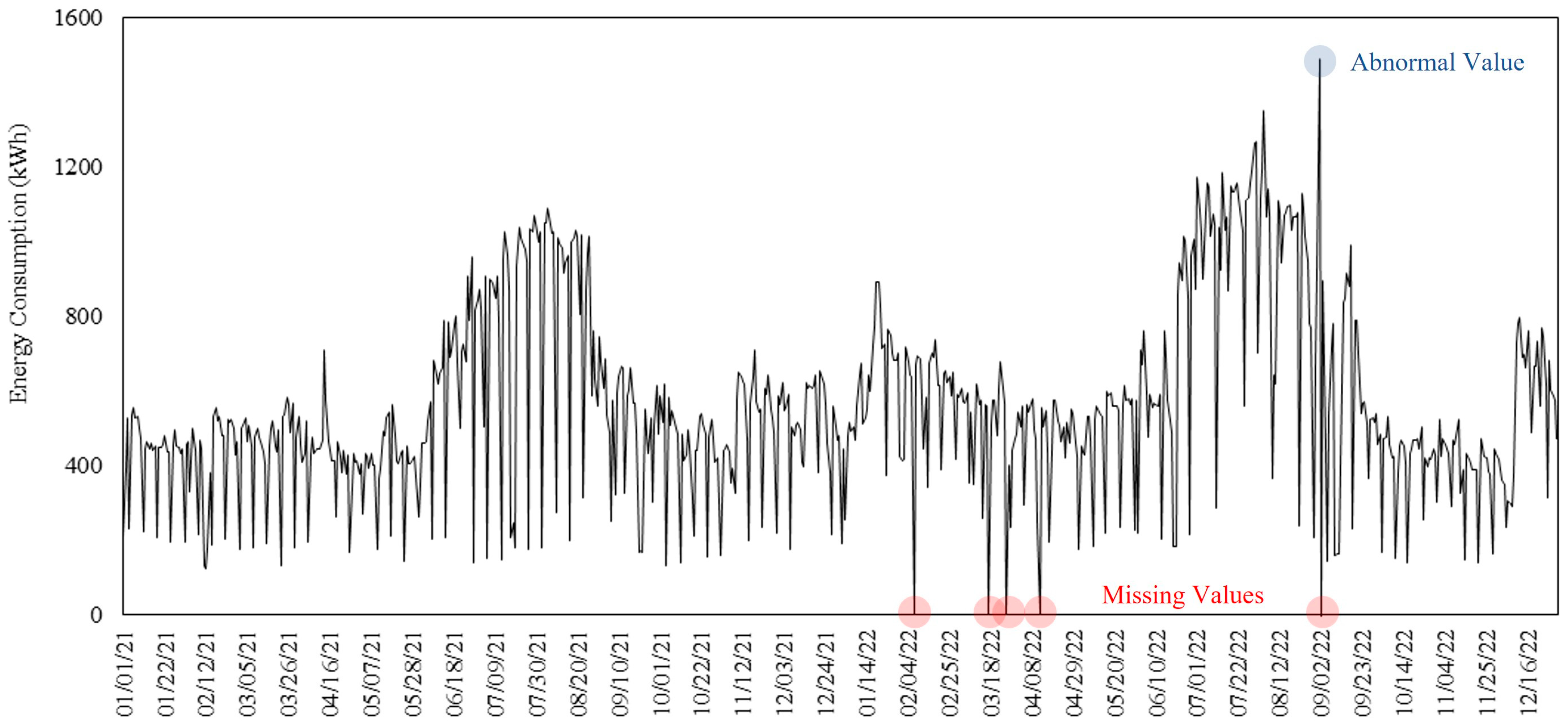
When investigating daily energy consumption of the case building throughout the observation period (Figure 3), there were distinct seasonal variations in daily energy consumption. The amount of daily energy consumption was higher during the summer months (e.g., June to August in 2021) than other seasons (e.g., September to November in 2021). Meanwhile, some energy use data had missing or abnormal values. To improve the quality of analysis, five missing data points were filled with the average value of energy spent before and after that day. In the case of abnormal data, it was excluded from analysis. In total, each time-series consisted of 729 data points.
In addition to the seasonal trend, the case building exhibited weekly energy use patterns (Figure 4). Energy consumption on Mondays was consistently lower than on other weekdays, which is likely attributable to the building’s scheduled closure on Mondays.
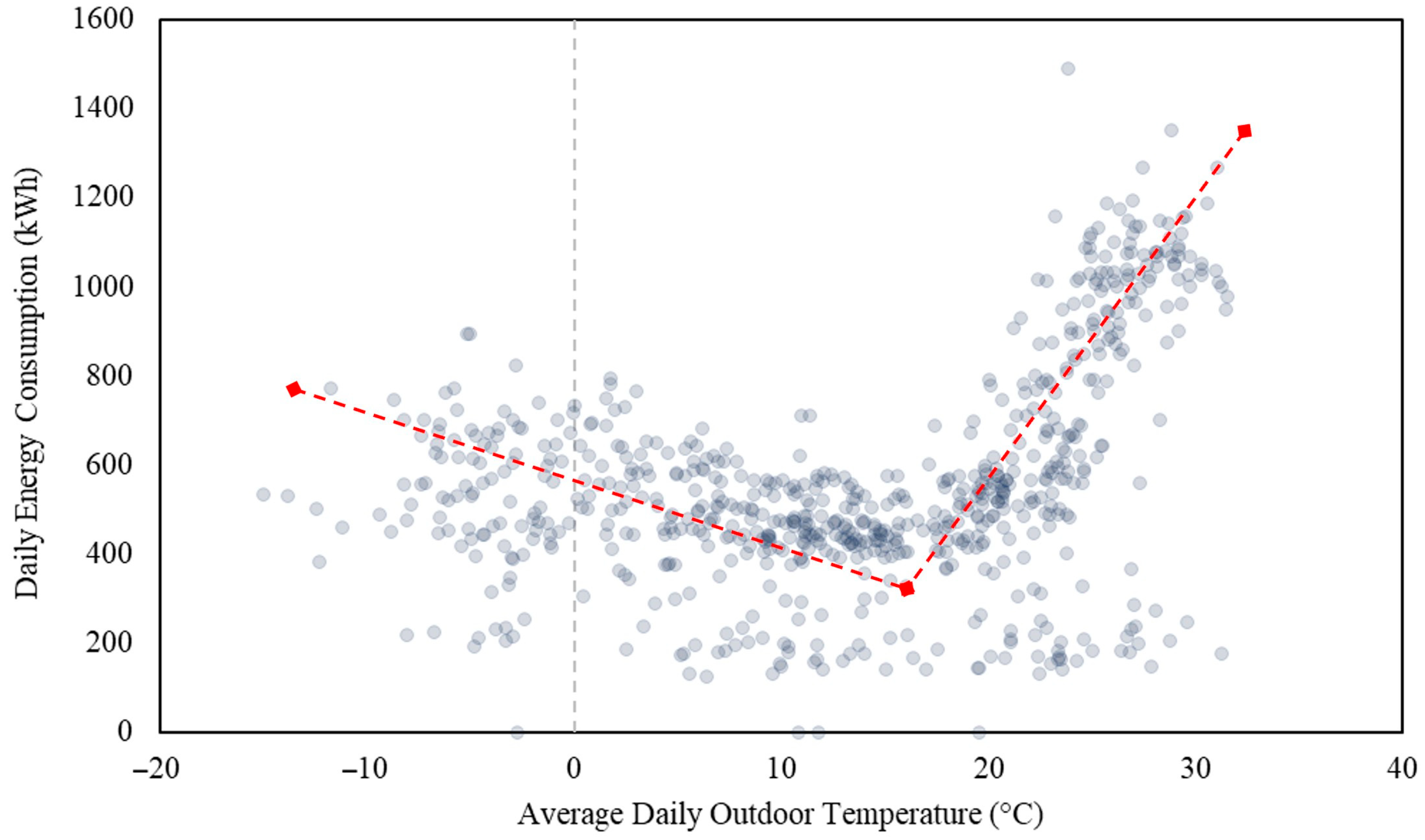
Looking closely at daily energy consumption across different daily average outdoor temperatures, there was an inverted U-shaped pattern in daily energy consumption (Figure 5). As outdoor temperature increased toward 18 °C, the total amount of daily energy spent in the case building was decreased. However, beyond 18 °C, energy consumption increased with an increase in outdoor temperature.
Moreover, a sensitivity analysis was conducted using Pearson correlation coefficients r to select significant predictors that affect the daily energy consumption of the case building. This analysis allows DL-based prediction models to use valid input variables during their development, thus improving the performance of energy use prediction [31]. For the sensitivity analysis, the following six variables were used: (1) average daily outdoor temperature, (2) average daily relative humidity, (3) average daily solar insolation, (4) day type, (5) temperature difference, and (6) daily energy consumption.
  • Average daily outdoor temperature (OT): Mean ambient temperature recorded outside the case building over a 24 h period and had numerical values (e.g., 17 °C),
  • Average daily relative humidity (RH): Mean atmospheric moisture content relative to the maximum possible at the same temperature, calculated over each day and has numerical values (e.g., 68%),
  • Average daily solar insolation (SI): Total incident solar radiation energy per unit area accumulated throughout the day and had numerical values (e.g., 185 kWh/m2),
  • Day type (DT): A categorical variable representing the day of the week with possible values including Monday (1), Tuesday (2), Wednesday (3), Thursday (4), Friday (5), Saturday (6), and Sunday (7),
  • Temperature difference (TD): Difference between average daily outdoor temperature and the 18 °C (e.g., −5 °C or 25 °C), and
  • Daily energy consumption (E): Total amount of energy consumed by the case building within a 24 h period (e.g., 24 kWh), which includes heating, cooling, lighting, plug loads, and equipment.
If X represents energy consumption and Y denotes a variable, the Pearson correlation coefficients r X , Y were calculated using Equation (1).
r X ,   Y = C o v ( X ,   Y ) σ X σ Y
where
  • C o v ( X , Y ) : Covariance of X and Y ,
  • σ X : Standard deviation of X , and
  • σ Y : Standard deviation of Y .
Figure 6 shows the results of the sensitivity analysis. The two temperature-related variables (OT and TD) showed a r of 0.36 with daily energy consumption (E), indicating a moderate positive correlation. The average daily relative humidity (RH) and day type (DT) had a r of 0.25 and 0.19, respectively, indicating a positive weak correlation with daily energy consumption (E). Conversely, the solar insolation (SI) exhibited a negligible correlation ( r = 0.01) with daily energy consumption (E). Therefore, the first four variables (i.e., OT, RH, DT, and TD) were considered as input variables of DL-based energy use prediction models.

4. Model Development

DL-based energy prediction models were developed to examine the effect of augmented input variables—derived through time-series decomposition—on the performance of building energy use prediction. For the data augmentation, an unobserved component model (UCM) was applied to the raw SEDC dataset. The UCM is a probabilistic decomposition method that separates a time series into interpretable temporal components—trend, seasonal, cycle, and irregular—based on state space modeling [32]. UCM has been extensively used in econometrics [33], climate analysis [34], and traffic volume prediction [35]. Compared to other decomposition methods (e.g., Seasonal-Trend decomposition using Loes, wavelet decomposition, or Empirical Mode Decomposition), UCM offers a model-based framework that enables statistically grounded and interpretable augmentation, which is particularly suitable for behavioral energy data with strong seasonal patterns. While UCM assumes linearity and may not capture complex nonlinear dynamics as effectively as deep learning-based approaches, its transparency and low risk of generating unrealistic artifacts make it a practical choice for this study. Moreover, the limitations of UCM are manageable in our context, as the data exhibits clear seasonal and trend structures, and model diagnostics confirmed the reliability of the decomposition.
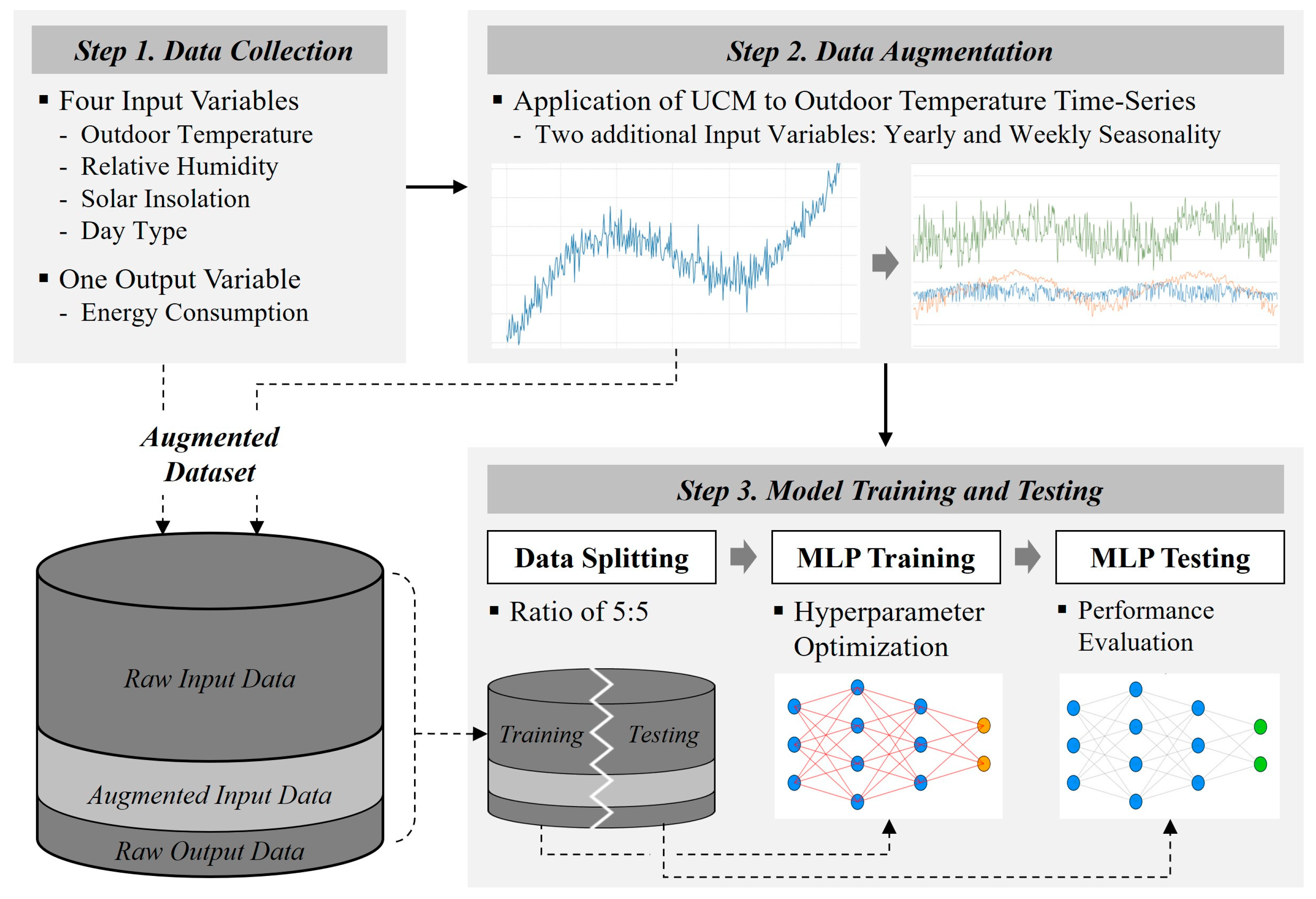
Figure 7 illustrates a process for developing the prediction models, which consisted of three main steps: (i) data acquisition, (ii) data augmentation, and (iii) model training and testing.

4.1. Data Acquisition

The model development began with collecting historical data from the raw SEDC dataset. As described in Section 4, average daily outdoor temperature, temperature difference, average daily relative humidity, and day type were employed as input variables for DL-based energy use prediction models due to their significant relationships with daily energy consumption. The variable daily energy consumption was used as an output of the proposed prediction model.

4.2. Data Augmentation

An augmented SEDC dataset was created by applying UCM to the raw SEDC dataset. In this study, the UCM-based time-series decomposition was conducted on average daily outdoor temperature for the following three reasons. First, outdoor temperature exhibits dynamic temporal patterns. Second, outdoor temperature data is readily available for predicting daily energy consumption of new buildings. Third, the correlation analysis confirmed that it exerted the strongest influence on daily energy consumption in the case building (Figure 6).
The decomposition of average daily outdoor temperature at time t ( y t ) can be conducted using Equation (2) and shown in Figure 8. All the components are estimated via maximum likelihood using Maximum Likelihood Estimation.
y t = μ t + γ t + Ψ t + i = 1 p ϕ i y i 1 + j = 1 m β j x j t + ε t
where
  • μ t : Trend component of outdoor temperature time-series which captures long-term changes overs time. This allowed us to flexibly capture long-term temperature trends that change over time,
  • γ t : Seasonality component of outdoor temperature time-series which represents recurring patterns within a year. To model the multiple seasonalities evident in the data, three stochastic seasonal factors with weekly (7 days), monthly (approximately 30 days), and yearly (365.25 days) cycles were used together,
  • Ψ t : Cyclical component of outdoor temperature time-series which reflects longer-term cycles,
  • i = 1 p ϕ i y i 1 : Autoregressive component which models the influence of past values of outdoor temperature time series on the current value,
  • j = 1 m β j x j t : Regression component of outdoor temperature time-series which capture the effect of external explanatory variables x j t , and
  • ε t : Irregular (noise) component of outdoor temperature time-series which accounts for random fluctuations not explained by the other components.
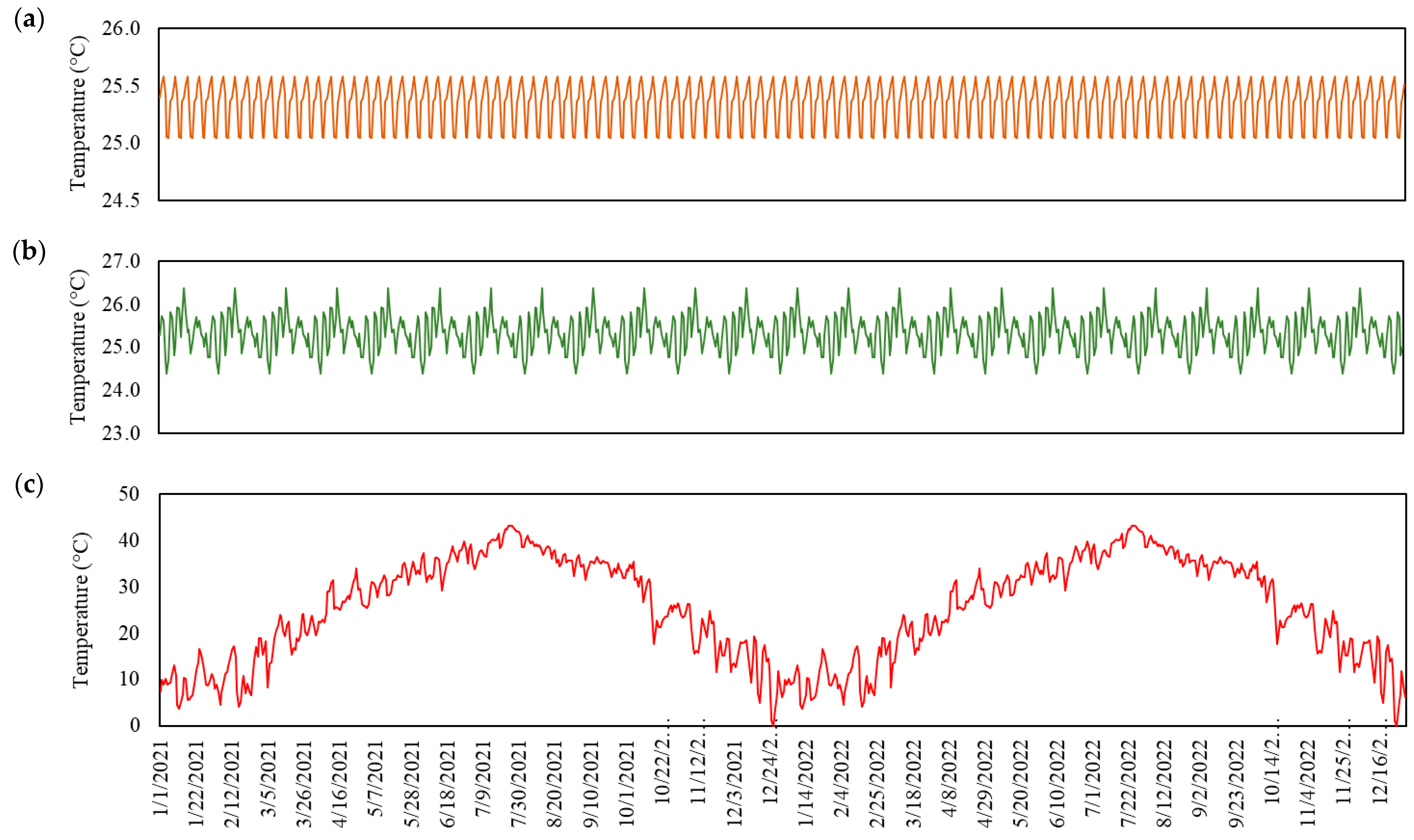
Figure 8. (a) Weekly, (b) monthly, and (c) yearly seasonality components of average daily outdoor temperature times series.
Buildings 15 03467 g008
Among the extracted components, the trend and cycle components were not used as additional input variables for the DL models. Unlike the seasonal component, outdoor temperature generally does not exhibit a clear trend and cycle unless considered over long-time horizons, which are not applicable for short-term forecasting (i.e., daily energy use prediction for new buildings). Moreover, although descriptive statistics on the seasonal components of UCM outputs revealed distinct patterns across different time scales, this did not lead to variations in daily energy consumption of the case building. Specifically, weekly seasonality (Figure 8a) was stable with a mean of 25.34 and minimal variability (variance = 0.038, SD = 0.20), suggesting a consistent weekly cycle. Similarly, monthly seasonality (Figure 8b) had a similar mean of 25.34 but slightly greater variance (variance = 0.205, SD = 0.45), indicating moderate fluctuations at the monthly level. Conversely, annual seasonality (Figure 8c) with a mean of 25.34 but significantly higher variability (variance = 117.81, SD = 10.85) exhibited significant heterogeneity ranging from 0.00 to 43.11. However, as shown in Figure 3, there was no significant variations in daily energy consumption within each month. Therefore, this study adopted only the yearly and weekly seasonality components ( γ t 365 and γ t 7 ) to construct the augmented SEDC dataset (i.e., additional input variables).

4.3. Model Training and Testing

Using the augmented SEDC dataset, DL–based energy prediction models were trained and tested to estimate daily building energy consumption. The prediction models were constructed using a multilayer perceptron (MLP) architecture rather than more complex recurrent networks such as Long Short-Term Memory (LSTM) [36,37] or Gated Recurrent Unit (GRU) [38] due to the limited size of the available training dataset. Since LSTM and GRU networks include substantially more parameters due to their gating mechanisms, they generally require larger datasets to avoid overfitting and to fully leverage their capacity for capturing long-term temporal dependencies. In contrast, the relatively simple architecture of MLPs is less prone to overfitting in data-scarce conditions and can yield more stable and reliable predictive performance. Therefore, given the scale of the augmented SEDC dataset and the objectives of this study, the MLP was considered the most appropriate modeling choice.
The MLP networks had six input nodes (OTt, RHt, DTt, TDt, γ t 365 , and γ t 7 ) which interact one output node (Et) through the mediation of multiple hidden nodes. Different numbers of hidden layers and nodes (Table 1) were considered for the development of the MLP networks due to its significant impact on the prediction performance. To further enhance model performance and prevent overfitting, several hyperparameters were systematically varied. First, different dropout rates were applied in conjunction with batch normalization during training. Second, various batch sizes were tested for fine-tuning. Third, the Adam optimizer with ReLU activation functions was employed across the hidden layers to optimize network parameters. In total, 16 MLP networks were developed for the prediction of average daily energy consumption.
For the model development, the augmented SEDC dataset was divided into training and test sets in a 50:50 ratio. Given that the dataset consisted of a two-year-long time series, this split allowed for evaluating how accurately the MLP networks trained using UCM-augmented time series data predict daily energy consumption for the following year.
The training dataset came from data collected from 2021 and was used during the training of MLP networks to optimize their parameters (e.g., weights and errors). After the network training was completed, the remaining dataset (i.e., data collected from 2022) was used to evaluate the generalization of the trained MLP networks. During the network training and testing, the performance of energy use prediction was assessed using mean absolute percentage error (MAPE) and coefficient of variation in the root mean square error (CvRMSE). MAPE provides an intuitive measure of average prediction accuracy in percentage terms, making it useful for comparing models across different datasets. CvRMSE is recommended by industry standards (e.g., ASHRAE Guideline 14 and IPMVP) as it emphasizes larger errors due to its squared error formulation and normalizes the root mean square error by the mean of the observed values. The performance evaluation indexes are described as follows:
M A P E = 1 n i = 1 n y i y ^ i y i
C v R M S E = R M S E y ¯ × 100
R M S E = i = 1 n ( y i y ^ i ) 2 n
where
  • y i : Actual energy consumption at time t,
  • y ^ i : Predicted energy consumption at time t,
  • y ¯ : Average value of actual energy consumption during the prediction period n.
In both metrics, lower values indicate better predictive performance as they reflect smaller deviations between predicted and actual energy use.

5. Results

The performance of multiple MLP networks which were developed using the raw and augmented SEDC datasets was evaluated to see the effect of newly created input time-series on the prediction performance. The computational environment for the experiment included an NVIDIA RTX 3090 GPU, Intel i9 processor, 32 GB of RAM, and Python 3.9 (programming language).

5.1. Prediction Performance by Dataset Type

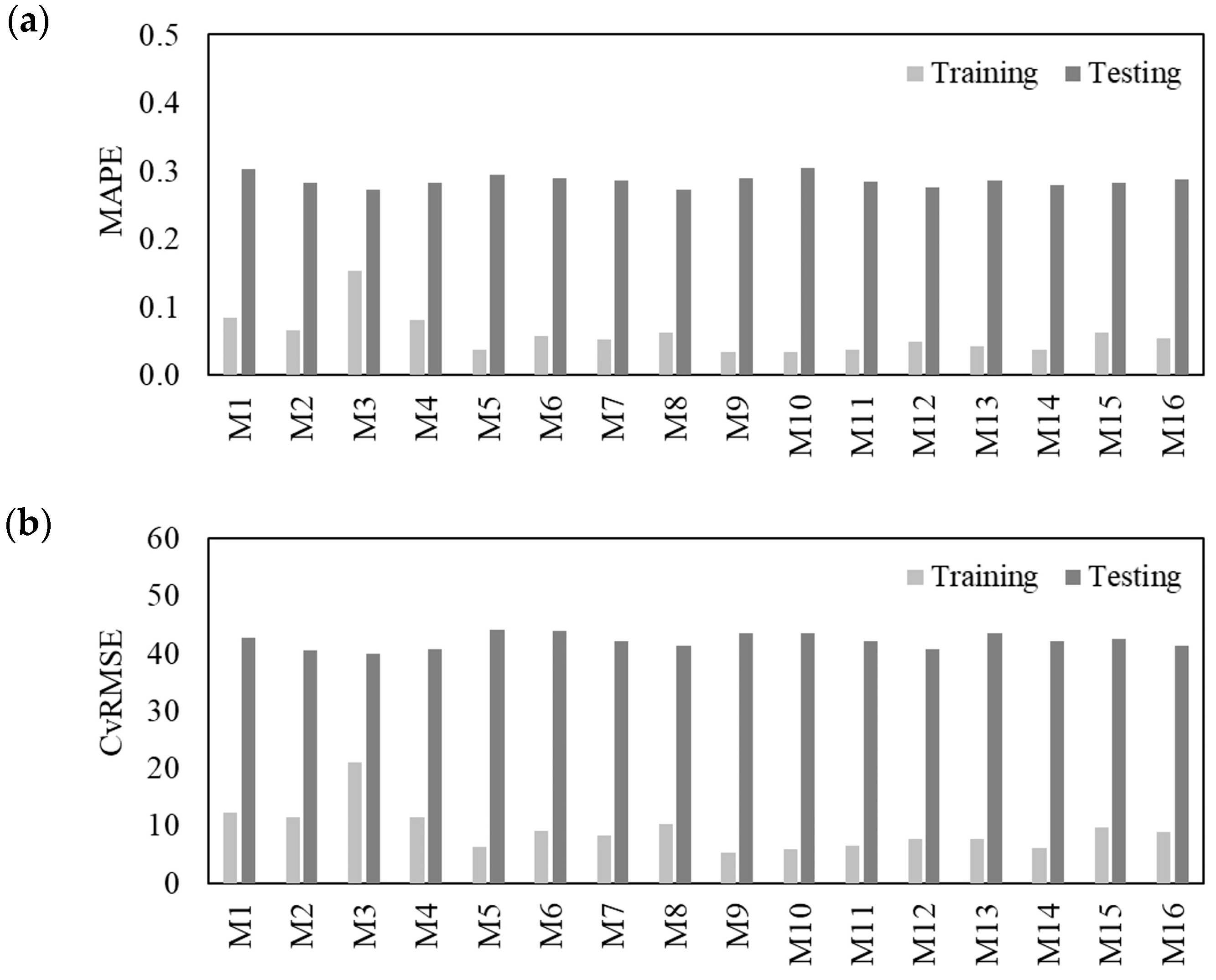
Figure 9 presents the performance results of the energy use prediction models which were trained and tested using the raw SEDC dataset. On average, the prediction performance of MLP networks was higher during training than during testing. The average MAPE values were 0.0716 (std: 0.0196) for training and 4.6577 (std: 0.0085) for testing. In the case of CvRMSE, the average values for training and testing were 11.0549 (std: 2.6179) and 43.2034 (std: 1.0318), respectively. Additionally, among the MLP networks evaluated during training, M9 produced the lowest MAPE and CvRMSE values of 0.0445 and 6.8189, respectively. However, when using the test dataset, the lowest MAPE value (0.2756) was observed for M4, while the lowest CvRMSE value (41.2179) was recorded for M3.
Figure 10 presents the evaluation results of the MLP networks which were developed using the augmented SEDC dataset. The results indicate that the MLP networks generally performed better during training than during testing. The average MAPE values were 0.0585 (std: 0.0297) for the training phase and 0.2854 (std: 0.0091) for the testing phase. Similarly, the average CvRMSE values were 9.2266 (std: 3.8094) for training and 42.1285 (std: 1.3234) for testing. Among all models, M9 demonstrated the best training performance, achieving the lowest MAPE and CvRMSE values of 0.0330 and 5.3500, respectively. In contrast, during testing, M8 exhibited the lowest MAPE (0.2722), while M3 produced the lowest CvRMSE (39.8096).
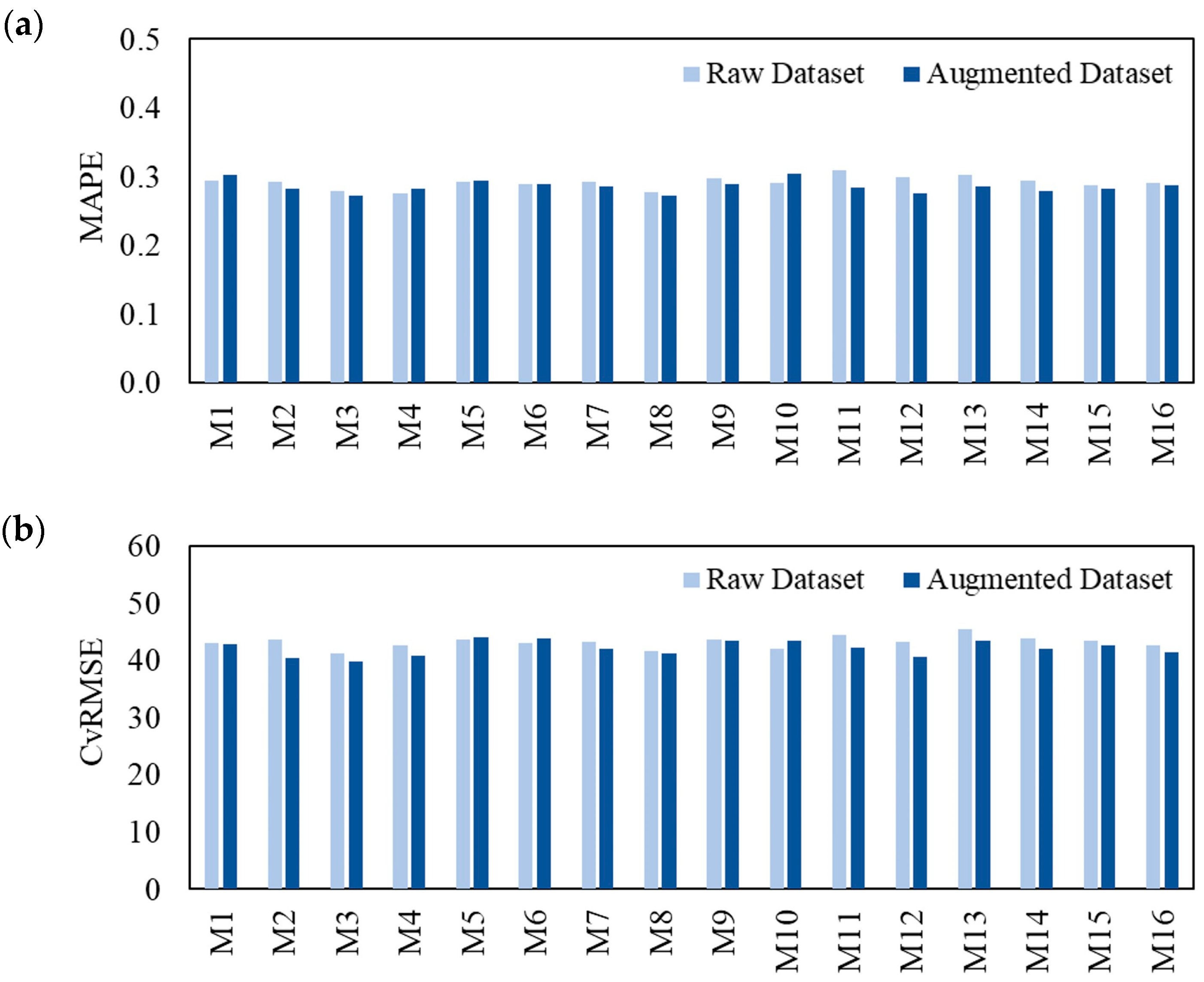
Figure 11 shows the testing performance of the MLP networks using the raw and augmented datasets. Across all the networks, the augmented dataset generally produced lower MAPE values compared to the raw dataset. The decrease in MAPE was particularly notable for M3, M8, M12, and M14. A similar trend was observed for CvRMSE, where most networks trained using the augmented dataset achieved lower values than those using raw dataset. The improvement was especially evident for M2, M3, M12, and M14.

5.2. Prediction Performance of Top-Performing MLP Network

Looking closely at the testing performance of the best MLP networks using the raw and augmented datasets, there was a 1.26% decrease in MAPE (0.2756 for M4 vs. 0.2722 for M8) and 3.42% decrease in CvRMSE (41.2179 for M3 vs. 39.8096 for M3).
When investigating the testing performance of the top-performing MLP networks under different configuration of additional input variables (i.e., γ t 365 and γ t 7 ), using both additional input variables produced the lowest values of MAPE (0.3114 for γ t 365 vs. 0.2997 for γ t 7 vs. 0.2722 for both variables). The values of CvRMSE were also lowest when the best MLP network was trained using both additional input variables (45.0548 for γ t 365 vs. 0.45.0308 for γ t 7 vs. 39.8096 for both variables).
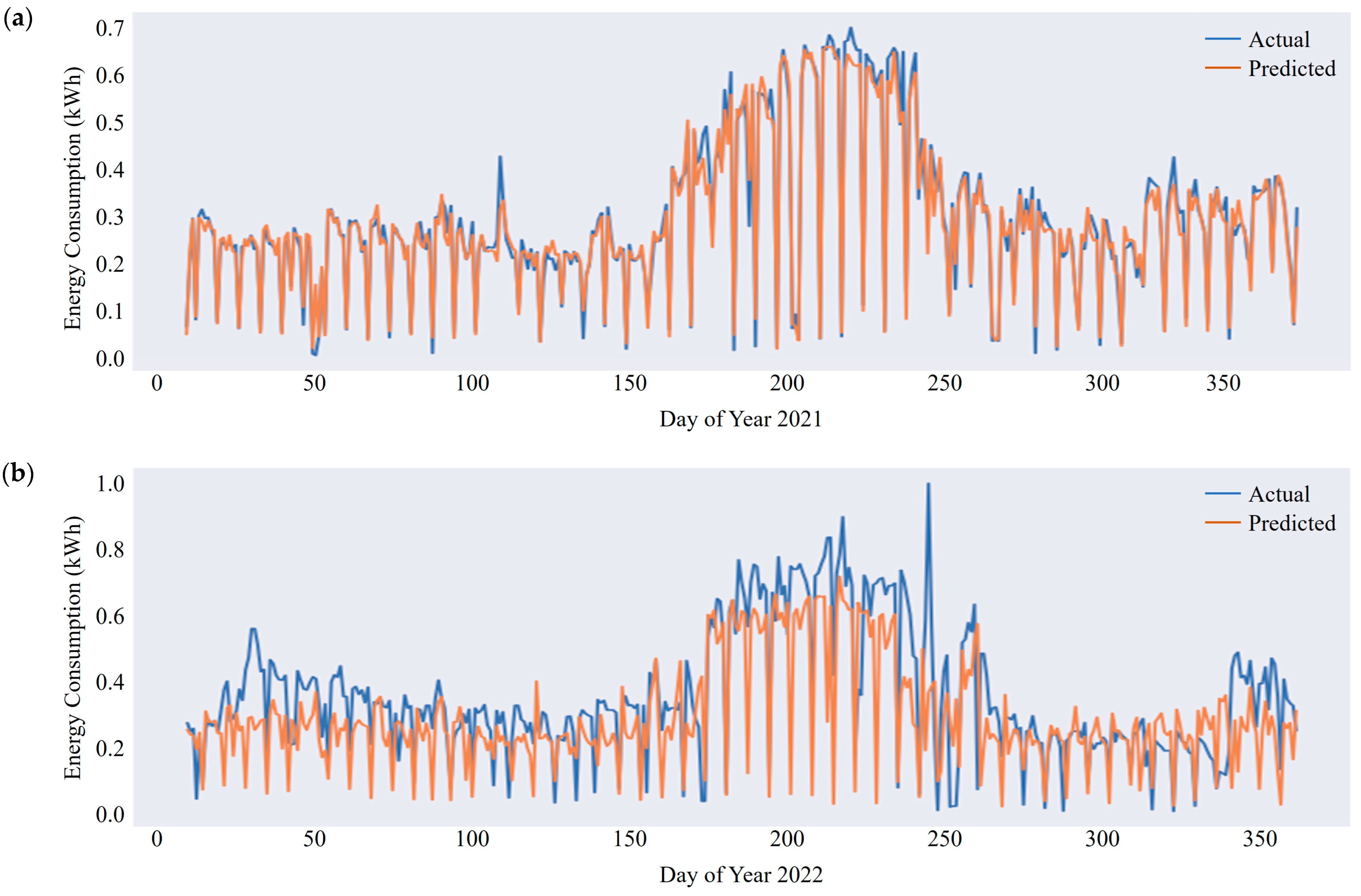
Additionally, the predicted consumption closely followed the seasonal and daily variations in the actual energy consumption (Figure 12a). For the testing year, the model successfully captured the general seasonal trends, such as the higher consumption during summer months, but occasional discrepancies were observed in the magnitude of daily fluctuations (Figure 12b). This discrepancy is attributed to the small data size of two years and the model training method, which targets time-series variables that indirectly influence the predictions. Nevertheless, we expect that UCM-based data augmentation for variables that indirectly influence energy use (e.g., outdoor temperature) will be beneficial for predicting energy consumption in new buildings.
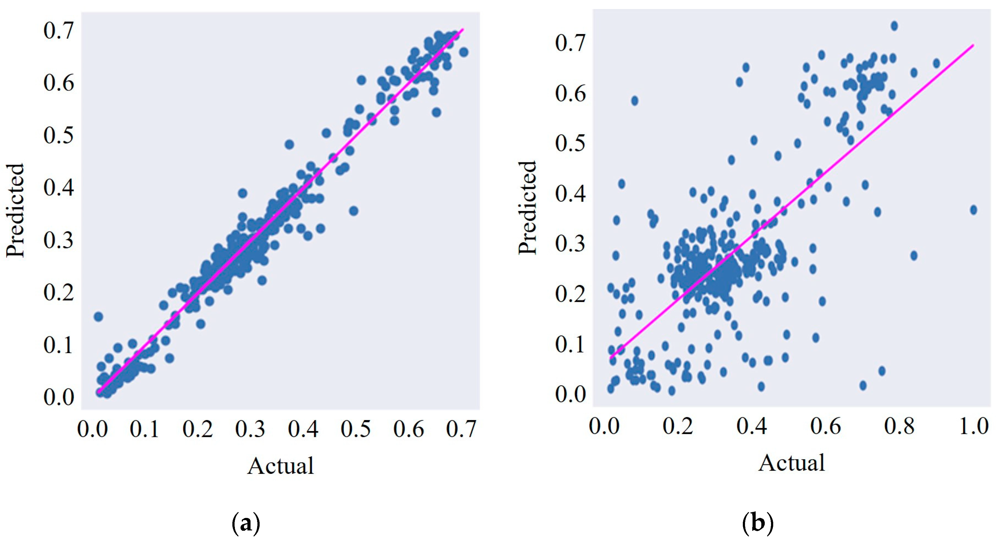
Furthermore, the predicted amount of daily energy consumption exhibited a strong linear relationship with the actual values, aligning closely along the 1:1 reference line (Figure 13a). These results indicate high predictive performance. In contrast, the testing results show greater variations between actual and predicted energy consumption with some degree of overestimation and underestimation observed across different consumption levels (Figure 13b).

6. Discussions

The prediction results demonstrate that augmenting the SEDC dataset through time-series decomposition and predictor expansion can enhance the performance of building energy consumption prediction models. Across the majority of MLP networks, the augmented dataset produced lower MAPE and CvRMSE values compared to the raw dataset, particularly in the testing phase. The observed improvements were most pronounced in M3, M8, M12, and M14, indicating that the additional temporal features derived from decomposition effectively improved the models’ prediction capabilities.
From the prediction results of the best-performing model (M3), it was found that while the training phase exhibited a strong linear relationship between predicted and actual values, testing results showed greater dispersion with both overestimations and underestimations across varying consumption levels. This indicates that despite the improvements gained through dataset augmentation, some level of overfitting to the training data remains, limiting generalization performance. The time-series comparisons also revealed that the model effectively captured broad seasonal patterns, such as increased consumption during summer months, but struggled to replicate the exact magnitude of daily fluctuations in the testing year.
These observations have important implications for the application of deep learning in building energy use prediction. First, the results highlight the potential of time-series decomposition as a low-cost, data-driven enhancement strategy, particularly when historical data is limited. Second, they emphasize the importance of balancing predictive accuracy and robustness. While the augmented dataset improved accuracy in most cases, residual performance gaps suggest that additional measures—such as incorporating operational schedules, occupancy data, or weather-related extreme events—may be necessary to fully capture complex consumption behaviors.
Additionally, although the improvements in prediction accuracy (1.26% MAPE and 3.42% CvRMSE) may appear modest, they were achieved solely by leveraging existing in-put variables through time-series decomposition without requiring additional data acquisition or costly resources. From a DSM perspective, even small gains in predictive accuracy can be practically significant as they enhance the reliability of consumption forecasts that inform large-scale operational decisions. When scaled across multiple buildings, such improvements may yield considerable benefits for energy providers and building operators. For energy providers, even a 3–4% reduction in forecast error can translate into more accurate load forecasting, enabling better alignment of supply with demand, reduced reliance on costly peaking power plants, and lower risks of grid instability during peak hours. For building operators, improved prediction accuracy can enhance scheduling of demand-side management strategies, such as pre-cooling or adjusting HVAC set-points, leading to lower utility bills and more efficient operation without sacrificing occupant comfort. In this sense, the modest improvements observed in this study highlight a low-cost and scalable pathway to achieve meaningful operational gains across the energy system.
This study has the following limitations that should be acknowledged and addressed in future research. First, the analysis was conducted on a single case building (SEDC), which constrains the generalizability of the findings. Different building types may exhibit unique operational patterns (e.g., occupancy schedules, equipment loads), and future research should therefore validate the proposed framework across a wider range of building types, climatic zones, and operational conditions to ensure broader applicability. Climatic zone differences, for instance, can alter the temporal dynamics of input variables such as outdoor air temperature, which in turn may influence the decomposition process and the predictive contribution of the derived components. Other environmental variables—such as relative humidity or solar insolation—may play a larger role in different climates. In such contexts, extending the decomposition process to additional variables could enhance the model’s ability to capture temporal dynamics and thereby improve prediction accuracy. Future research should explore such extensions.
Second, according to ASHRAE guidelines [39], the acceptable error threshold (CvRMSE) for daily building energy consumption prediction is typically set below 25%. Although the predictive performance reported in this study does not meet this benchmark (Figure 11b) and shows a large deviation between the actual and predicted values (Figure 12b), the primary objective was not to achieve state-of-the-art accuracy but rather to investigate how additional input variables—derived from readily available time-series decomposition—affect model performance. The results demonstrate that incorporating decomposition-based features contributes to measurable improvements in forecasting accuracy (Figure 11), thereby validating the methodological contribution of this approach. It is also acknowledged that the limited number of input variables likely constrained the model’s accuracy. Future research incorporating additional inputs, particularly occupancy-related variables that are widely recognized as critical determinants of energy consumption, has strong potential to substantially enhance predictive accuracy and enable compliance with ASHRAE benchmarks. However, despite these limitations, this study demonstrates the feasibility of enhancing building energy consumption prediction through time-series decomposition and highlights a pathway for improving model robustness by incorporating additional context-specific variables and broader validation efforts.
Third, the raw SEDC dataset contained only five isolated missing/anomalous daily observations, making it possible to apply the average of the adjacent days. When missingness is larger, clustered, or systematically related to covariates, deep learning–based reconstruction (e.g., Gated Recurrent Unit with Decay [40] or Deep Autoencoder Imputation [41]) may provide additional accuracy by capturing nonlinear temporal and cross-feature dependencies. Future work will explore such methods for data recovery, particularly under scenarios with extended outages or structured gaps.

7. Conclusions

This study proposed a deep learning-based energy use prediction framework which facilitates input data augmentation using the unobserved component model. To evaluate the performance of the proposed prediction performance, two years of historical data on energy consumption and environmental conditions was collected from a case building. The main findings are threefold. First, deep learning networks achieved a higher prediction performance during training than during testing. Second, testing performance was generally better when using the augmented dataset than the raw dataset. Third, the proposed data augmentation method contributes to a 1.26% decrease in MAPE and a 3.42% decrease in CvRMSE.
This research contributes to the literature by enhancing our understanding of how newly created predictors—derived from the decomposition of existing time-series—affect the performance of building energy use prediction. In addition, the proposed framework demonstrates that leveraging existing environmental data to generate additional input variables can improve predictive performance even when historical records are limited. However, as this study focused on a single case building, the generalizability of the findings remains constrained. Future research should extend the validation to multiple buildings in diverse climatic and operational contexts to confirm the broader applicability of the approach. Such efforts can also inform the design of more effective demand-side management programs based on more accurate prediction results.

Author Contributions

Conceptualization, T.K. and K.S.; methodology, T.K.; validation, T.K.; formal analysis, T.K.; investigation, T.K. and K.S.; data curation, T.K.; writing—original draft preparation, T.K. and K.S.; writing—review and editing, T.K. and K.S.; visualization, T.K. and K.S. All authors have read and agreed to the published version of the manuscript.

Funding

This research was supported by the National Research Foundation of Korea (NRF) grant funded by the Korea government (MSIT) (RS-2020-NR049539).

Data Availability Statement

The original contributions presented in this study are included in the article. Further inquiries can be directed to the corresponding author.

Acknowledgments

We thank Suwon Song, Korea Institute of Civil Engineering and Building Technology, for his assistance with the data collection.

Conflicts of Interest

The authors declare no conflicts of interest.

References

  1. Korea Energy Economics Institute. Energy Status of Korea 2023; Korea Energy Economics Institute: Ulsan, Republic of Korea, 2023. [Google Scholar]
  2. Nasir, T.; Bukhari, S.S.H.; Raza, S.; Munir, H.M.; Abrar, M.; Muqeet, H.A.U.; Bhatti, K.L.; Ro, J.S.; Masroor, R. Recent Challenges and Methodologies in Smart Grid Demand Side Management: State-of-the-Art Literature Review. Math. Probl. Eng. 2021, 2021, 5821301. [Google Scholar] [CrossRef]
  3. U.S. Energy Information Administration Demand-Side Management Programs Save Energy and Reduce Peak Demand. Available online: https://www.eia.gov/ (accessed on 2 March 2023).
  4. Chen, C.F.; Xu, X.; Cao, Z.; Mockus, A.; Shi, Q. Analysis of Social–Psychological Factors and Financial Incentives in Demand Response and Residential Energy Behavior. Front. Energy Res. 2023, 11, 932134. [Google Scholar] [CrossRef]
  5. Song, K.; Kwon, N.; Anderson, K.; Park, M.; Lee, H.-S.; Lee, S. Predicting Hourly Energy Consumption in Buildings Using Occupancy-Related Characteristics of End-User Groups. Energy Build. 2017, 156, 121–133. [Google Scholar] [CrossRef]
  6. Neto, A.H.; Fiorelli, F.A.S. Comparison between Detailed Model Simulation and Artificial Neural Network for Forecasting Building Energy Consumption. Energy Build. 2008, 40, 2169–2176. [Google Scholar] [CrossRef]
  7. Yun, K.; Luck, R.; Mago, P.J.; Cho, H. Building Hourly Thermal Load Prediction Using an Indexed ARX Model. Energy Build. 2012, 54, 225–233. [Google Scholar] [CrossRef]
  8. Li, K.; Hu, C.; Liu, G.; Xue, W. Building’s Electricity Consumption Prediction Using Optimized Artificial Neural Networks and Principal Component Analysis. Energy Build. 2015, 108, 106–113. [Google Scholar] [CrossRef]
  9. Guo, J.; Lin, P.; Zhang, L.; Pan, Y.; Xiao, Z. Dynamic Adaptive Encoder-Decoder Deep Learning Networks for Multivariate Time Series Forecasting of Building Energy Consumption. Appl. Energy 2023, 350, 121803. [Google Scholar] [CrossRef]
  10. Fang, L.; He, B. A Deep Learning Framework Using Multi-Feature Fusion Recurrent Neural Networks for Energy Consumption Forecasting. Appl. Energy 2023, 348, 121563. [Google Scholar] [CrossRef]
  11. Heidari, A.; Khovalyg, D. Short-Term Energy Use Prediction of Solar-Assisted Water Heating System: Application Case of Combined Attention-Based LSTM and Time-Series Decomposition. Sol. Energy 2020, 207, 626–639. [Google Scholar] [CrossRef]
  12. Gao, Y.; Ruan, Y. Interpretable Deep Learning Model for Building Energy Consumption Prediction Based on Attention Mechanism. Energy Build. 2021, 252, 111379. [Google Scholar] [CrossRef]
  13. Dong, Z.; Liu, J.; Liu, B.; Li, K.; Li, X. Hourly Energy Consumption Prediction of an Office Building Based on Ensemble Learning and Energy Consumption Pattern Classification. Energy Build. 2021, 241, 110929. [Google Scholar] [CrossRef]
  14. Shakeel, H.M.; Iram, S.; Hill, R.; Athar Farid, H.M.; Sheikh-Akbari, A.; Saleem, F. A Machine Learning-Based Intelligent Framework for Predicting Energy Efficiency in Next-Generation Residential Buildings. Buildings 2025, 15, 1275. [Google Scholar] [CrossRef]
  15. Riyadh Baqer, N.; Rashidi-Khazaee, P. Residential Building Energy Usage Prediction Using Bayesian-Based Optimized XGBoost Algorithm. IEEE Access 2025, 13, 36036–36049. [Google Scholar] [CrossRef]
  16. Harvey, A.C.; Peters, S. Estimation Procedures for Structural Time Series Models. J. Forecast. 1990, 9, 89–108. [Google Scholar] [CrossRef]
  17. Jiao, Y.; Tan, Z.; Zhang, D.; Zheng, Q.P. Short-Term Building Energy Consumption Prediction Strategy Based on Modal Decomposition and Reconstruction Algorithm. Energy Build. 2023, 290, 113074. [Google Scholar] [CrossRef]
  18. Masrur Ahmed, A.A.; Bailek, N.; Abualigah, L.; Bouchouicha, K.; Kuriqi, A.; Sharifi, A.; Sareh, P.; Al khatib, A.M.G.; Mishra, P.; Colak, I.; et al. Global Control of Electrical Supply: A Variational Mode Decomposition-Aided Deep Learning Model for Energy Consumption Prediction. Energy Rep. 2023, 10, 2152–2165. [Google Scholar] [CrossRef]
  19. Li, F.; Wan, Z.; Koch, T.; Zan, G.; Li, M.; Zheng, Z.; Liang, B. Improving the Accuracy of Multi-Step Prediction of Building Energy Consumption Based on EEMD-PSO-Informer and Long-Time Series. Comput. Electr. Eng. 2023, 110, 108845. [Google Scholar] [CrossRef]
  20. Wei, S.; Bai, X. Multi-Step Short-Term Building Energy Consumption Forecasting Based on Singular Spectrum Analysis and Hybrid Neural Network. Energies 2022, 15, 1743. [Google Scholar] [CrossRef]
  21. Chou, S.Y.; Dewabharata, A.; Zulvia, F.E.; Fadil, M. Forecasting Building Energy Consumption Using Ensemble Empirical Mode Decomposition, Wavelet Transformation, and Long Short-Term Memory Algorithms. Energies 2022, 15, 1035. [Google Scholar] [CrossRef]
  22. Fernández-Martínez, D.; Jaramillo-Morán, M.A. Multi-Step Hourly Power Consumption Forecasting in a Healthcare Building with Recurrent Neural Networks and Empirical Mode Decomposition. Sensors 2022, 22, 3664. [Google Scholar] [CrossRef] [PubMed]
  23. Zhang, J.; Huang, M.; Wan, N.; Deng, Z.; He, Z.; Luo, J. Missing Measurement Data Recovery Methods in Structural Health Monitoring: The State, Challenges and Case Study. Measurement 2024, 231, 114528. [Google Scholar] [CrossRef]
  24. Chai, J.; Zeng, H.; Li, A.; Ngai, E.W.T. Deep Learning in Computer Vision: A Critical Review of Emerging Techniques and Application Scenarios. Mach. Learn. Appl. 2021, 6, 100134. [Google Scholar] [CrossRef]
  25. Rojas-Carabali, W.; Agrawal, R.; Gutierrez-Sinisterra, L.; Baxter, S.L.; Cifuentes-González, C.; Wei, Y.C.; Abisheganaden, J.; Kannapiran, P.; Wong, S.; Lee, B.; et al. Natural Language Processing in Medicine and Ophthalmology: A Review for the 21st-Century Clinician. Asia-Pac. J. Ophthalmol. 2024, 13, 100084. [Google Scholar] [CrossRef]
  26. Lian, H.; Wei, H.; Wang, X.; Chen, F.; Ji, Y.; Xie, J. Research on Real-Time Energy Consumption Prediction Method and Characteristics of Office Buildings Integrating Occupancy and Meteorological Data. Buildings 2025, 15, 404. [Google Scholar] [CrossRef]
  27. Guo, Y.; Liu, Y.; Wang, Y.; Du, C.; Li, H.; Zhang, Z. A Deep Belief Network-Based Energy Consumption Prediction Model for Water Source Heat Pump System. Appl. Therm. Eng. 2024, 255, 124000. [Google Scholar] [CrossRef]
  28. Tian, Z.; Chen, D.; Zhao, L. Short-Term Energy Consumption Prediction of Large Public Buildings Combined with Data Feature Engineering and Bilstm-Attention. Appl. Sci. 2024, 14, 2137. [Google Scholar] [CrossRef]
  29. Jana, R.K.; Ghosh, I.; Sanyal, M.K. A Granular Deep Learning Approach for Predicting Energy Consumption. Appl. Soft Comput. 2020, 89, 106091. [Google Scholar] [CrossRef]
  30. Zheng, P.; Zhou, H.; Liu, J.; Nakanishi, Y. Interpretable Building Energy Consumption Forecasting Using Spectral Clustering Algorithm and Temporal Fusion Transformers Architecture. Appl. Energy 2023, 349, 121607. [Google Scholar] [CrossRef]
  31. Yadav, A.K.; Chandel, S.S. Identification of Relevant Input Variables for Prediction of 1-Minute Time-Step Photovoltaic Module Power Using Artificial Neural Network and Multiple Linear Regression Models. Renew. Sustain. Energy Rev. 2017, 77, 955–969. [Google Scholar] [CrossRef]
  32. Harvey, A.C. Forecasting, Structural Time Series Models and the Kalman Filter; Cambridge University Press: Cambridge, UK, 1989. [Google Scholar]
  33. Maddala, G.S.; Nimalendran, M. An Unobserved Component Panel Data Model to Study the Effect of Earnings Surprises on Stock Prices, Trading Volumes, and Spreads. J. Econ. 1995, 68, 229–242. [Google Scholar] [CrossRef]
  34. Smith, W.R.; Bauserman, R.L.; Ballas, S.K.; McCarthy, W.F.; Steinberg, M.H.; Swerdlow, P.S.; Waclawiw, M.A.; Barton, B.A. Climatic and Geographic Temporal Patterns of Pain in the Multicenter Study of Hydroxyurea. Pain 2009, 146, 91–98. [Google Scholar] [CrossRef] [PubMed]
  35. Bian, Z.; Zhang, Z.; Liu, X.; Qin, X. Unobserved Component Model for Predicting Monthly Traffic Volume. J. Transp. Eng. A Syst. 2019, 145, 04019052. [Google Scholar] [CrossRef]
  36. Hochreiter, S.; Schmidhuber, J. Long Short-Term Memory. Neural Comput. 1997, 9, 1735–1780. [Google Scholar] [CrossRef] [PubMed]
  37. Elhabyb, K.; Baina, A.; Bellafkih, M.; Deifalla, A.F. Machine Learning Algorithms for Predicting Energy Consumption in Educational Buildings. Int. J. Energy Res. 2024, 2024, 6812425. [Google Scholar] [CrossRef]
  38. Chung, J.; Gulcehre, C.; Cho, K.; Bengio, Y. Empirical Evaluation of Gated Recurrent Neural Networks on Sequence Modeling. arXiv 2014, arXiv:1412.3555. [Google Scholar] [CrossRef]
  39. American Society of Heating, Refrigerating, and Air-Conditioning Engineers (ASHRAE). ASHRAE Handbook Fundamentals; American Society of Heating, Refrigerating, and Air-Conditioning Engineers (ASHRAE): Atlanta, GA, USA, 2009. [Google Scholar]
  40. Sasu, G.-V.; Ciubotaru, B.-I.; Goga, N.; Vasilățeanu, A. Addressing Missing Data Challenges in Geriatric Health Monitoring: A Study of Statistical and Machine Learning Imputation Methods. Sensors 2025, 25, 614. [Google Scholar] [CrossRef]
  41. Xu, D.; Hu, P.J.-H.; Fang, X. Deep Learning-Based Imputation Method to Enhance Crowdsourced Data on Online Business Directory Platforms for Improved Services. J. Manag. Inf. Syst. 2023, 40, 624–654. [Google Scholar] [CrossRef]
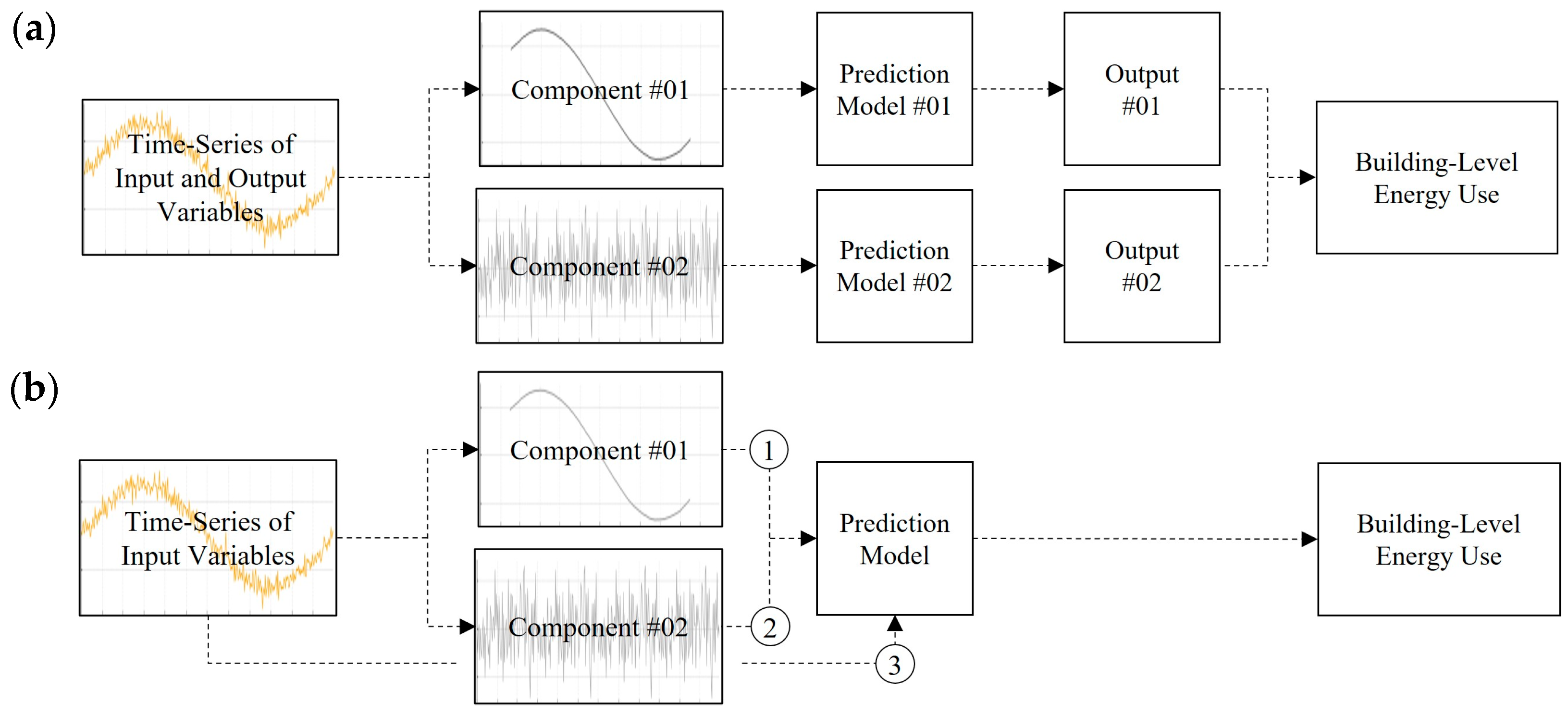
Figure 1. Utilization of time-series decomposition for building energy use prediction: (a) prediction model segmentation and (b) augmentation of input variables.
Buildings 15 03467 g001
Figure 2. (a) Side and (b) aerial views of Seoul Energy Dream Center.
Buildings 15 03467 g002
Figure 3. Daily energy consumption of Seoul Energy Dream Center in 2021 and 2022.
Buildings 15 03467 g003
Figure 4. Average daily energy consumption of Seoul Energy Dream Center by day of the observation period.
Buildings 15 03467 g004
Figure 5. Average daily outdoor temperature by daily energy consumption of Seoul Energy Dream Center in 2021 and 2022.
Buildings 15 03467 g005
Figure 6. Pearson’s correlation coefficients of average daily outdoor temperature (OT), average daily relative humidity (RH), average daily solar insolation (SI), day type (DT), temperature difference (TD), and daily energy consumption (E).
Buildings 15 03467 g006
Figure 7. Process of developing deep learning-based energy use prediction models using the augmented SEDC dataset.
Buildings 15 03467 g007
Figure 9. (a) MAPE and (b) CvRMSE Values of MLP Networks using Raw SEDC Dataset.
Buildings 15 03467 g009
Figure 10. (a) MAPE and (b) CvRMSE Values of MLP Networks using Augmented SEDC Dataset.
Buildings 15 03467 g010
Figure 11. (a) MAPE and (b) CvRMSE values of the MLP networks evaluated with test datasets derived from the raw and augmented SEDC datasets.
Buildings 15 03467 g011
Figure 12. Actual and predicted daily energy consumption by day of years when M3 was (a) trained and (b) tested using the augmented SEDC dataset.
Buildings 15 03467 g012
Figure 13. Actual and predicted daily energy consumption when M3 was (a) trained and (b) tested using the augmented SEDC dataset.
Buildings 15 03467 g013
Table 1. Building Energy Prediction Model Architecture.
NoNumber of Nodes in Hidden LayersDropoutBatch Size
M1[12, 16, 32, 16, 12, 6]0.0032
M264
M30.0132
M464
M5[18, 24, 48, 24, 18, 12]0.0032
M664
M70.0132
M864
M9[24, 32, 64, 32, 24, 18]0.0032
M1064
M110.0132
M1264
M13[12, 16, 32, 64, 32, 16, 12]0.0032
M1464
M150.0132
M1664
Disclaimer/Publisher’s Note: The statements, opinions and data contained in all publications are solely those of the individual author(s) and contributor(s) and not of MDPI and/or the editor(s). MDPI and/or the editor(s) disclaim responsibility for any injury to people or property resulting from any ideas, methods, instructions or products referred to in the content.