Efficient Lightweight CNN and 2D Visualization for Concrete Crack Detection in Bridges

Abstract

The durability and safety of modern concrete architecture and infrastructure are critically impacted by early-stage surface cracks. Timely and appropriate identification and management of these cracks are therefore essential to enhance structural longevity and stability. This study utilizes computer vision technology to construct a large-scale database, comprising 106,998 concrete surface crack images from various research sources. Through data augmentation, the database is extended to 140,000 images to fully leverage the advantages of deep learning models. For concrete surface crack detection, this study proposed a lightweight convolutional neural network (CNN) model, achieving 92.27% accuracy, 94.98% recall, and a 92.39% F1 score. Notably, the model runs smoothly on lightweight office notebooks without GPUs. Additionally, an image stitching algorithm that seamlessly stitches multiple images was proposed to generate high-quality panoramic views of bridges. The image stitching algorithm demonstrates robustness when applied to multiple images, successfully achieving stitching without visible seams or errors, providing efficient and reliable technical support for bridge panorama generation. The research outcomes demonstrate significant practical value in bridge inspection, providing robust technical support for safe and efficient bridge inspection. Moreover, our findings offer valuable references for future research and applications in related fields.

1. Introduction

The increasing demand for efficient damage detection, condition assessment, and maintenance of bridge structures stems from their aging, long-term environmental effects, and growing traffic loads, leading to prevalent bridge-related issues [1]. Monitoring, testing, and reinforcement present major challenges for urban management. Consequently, the efficient and intelligent detection of bridge diseases is vital for maintenance [2]. Considering the large number of old bridges, it is impractical to individually install sophisticated structural health monitoring systems. Hence, the development of a fast and cost-effective disease detection method for a substantial quantity of small and medium-sized concrete bridges holds great significance.

Since the late 20th century, computer vision technology has demonstrated gradual advantages in structural monitoring, offering high accuracy, long-distance capability, ease of implementation, and low cost. It enables millimeter-level precision in measuring structural dynamic displacements over kilometer-scale distances [3,4]. Driven by the Internet of Things (IoT) and artificial intelligence (AI) technologies, the automation and intelligent maintenance of bridges have become widely recognized focal points [5,6,7]. To overcome the limitations of traditional bridge inspection methods, scholars have been continuously exploring the deep integration of AI technology with bridge inspection.

Unmanned Aerial Vehicles (UAVs), recognized as flexible, efficient, and cost-effective platforms, have become widely used in various disciplines, including civil engineering, surveying, and geotechnical engineering. By combining UAVs with computer vision technology, it is possible to quickly acquire information about the bridge’s operating environment, operational loads, and structural response status, enabling the assessment of bridge structural condition and safety performance and providing support for making scientifically sound decisions on bridge maintenance and management. It has been a hot topic and vision for researchers worldwide to keep pace with the development trends in computer science and apply these new technologies to the field of bridge inspection [8,9].

With the gradual maturity of computer vision technology, an increasing number of scholars have applied it to engineering fields, particularly in the identification of structural surface defects. Deep learning methods, compared to traditional image processing techniques, offer higher recognition accuracy in complex environments. Some researchers have applied deep learning techniques to tasks such as crack detection and achieved significant progress. Liu [10] proposed a multiscale damage identification method that combines structural dynamic indicators and crack indicators for overall and local damage recognition. Wang and Qi [11] selected effective crack features and established an automatic discrimination models, which showed that the models exhibited good adaptability, efficiently achieving crack recognition and further validating the necessity of crack feature allocation. Han and Zhao [12] proposed a crack detection method that involved preprocessing crack images using bilateral filtering and three-stage linear transformations to enhance crack edge recognition accuracy. Additionally, an improved edge gradient method was employed for crack width positioning and automatic retrieval. Fan et al. [13] presented a crack detection algorithm based on mid-scale geometric features, which achieved an accuracy of 93.3%, making it suitable for small-sample engineering. Zhang et al. [14] developed a U-Net model, utilizing the generalized dice loss function to improve crack detection accuracy, outperforming other methods. Cha et al. [15] trained a convolutional neural network (CNN) using a dataset of 40,000 crack images. Compared to traditional Canny and Sobel edge detection algorithms, their approach demonstrated higher accuracy and stronger robustness in crack recognition. Liu et al. [16] applied a mask-based CNN for automatic detection and segmentation of small cracks in asphalt pavements. Deng et al. [17] proposed a crack detection method with deformable modules based on R-CNN, which effectively detects out-of-plane cracks that conventional detectors may struggle to identify.

But the methods often have high requirements for computing power and storage devices, leading to increased hardware costs and making them unsuitable for practical application environments of small and medium-sized bridges. The rapid development of computer vision, image processing technology has driven advancements in the visualization of detection results [18,19,20,21]. The goal of visualization techniques is to provide engineers and maintenance units with intuitive and easy-to-understand detection results [19,20]. Image stitching techniques, combined with efficient image acquisition tools like drones, can help comprehensively and systematically grasp the usage condition of bridges, thereby supporting the development of scientifically sound maintenance strategies [21,22,23]. Image stitching technology combines multiple images with overlapping regions to create a large-field-of-view two-dimensional panoramic image. This technique provides a wider perspective and facilitates in-depth observation and analysis of the overall appearance of a bridge component [24]. Building upon the locally captured crack images from drones, image stitching technology can generate a complete overview of the cracks, enabling engineers and maintenance units to have a comprehensive understanding of the current state of crack development and its impact on the stability of the bridge structure [25,26].

The main focus of this study is to propose a lightweight detection method for concrete bridge cracks using computer vision technology. It aims to address the detection needs of medium and small bridges from a qualitative classification perspective. Additionally, the study incorporates image stitching algorithms to achieve two-dimensional visualization of the detection results and provide an image-based information model of the local components.

2. Materials and Methods

To provide a comprehensive overview of our research methodology and to illustrate the logical progression of the study, the overall workflow is presented in Figure 1. This diagram outlines the key stages, from initial concrete image data preparation and lightweight CNN-based crack detection to image stitching for panoramic views and finally, integrated 2D visualization with crack annotations.

In the field of computer vision and deep learning research, datasets play a crucial role in model training and evaluation. Especially in image recognition and processing tasks, representative and high-quality datasets not only provide abundant sample data but also offer a unified benchmark for performance comparison among different algorithms, laying a crucial foundation for the rapid advancement of computer vision and deep learning technologies [27].

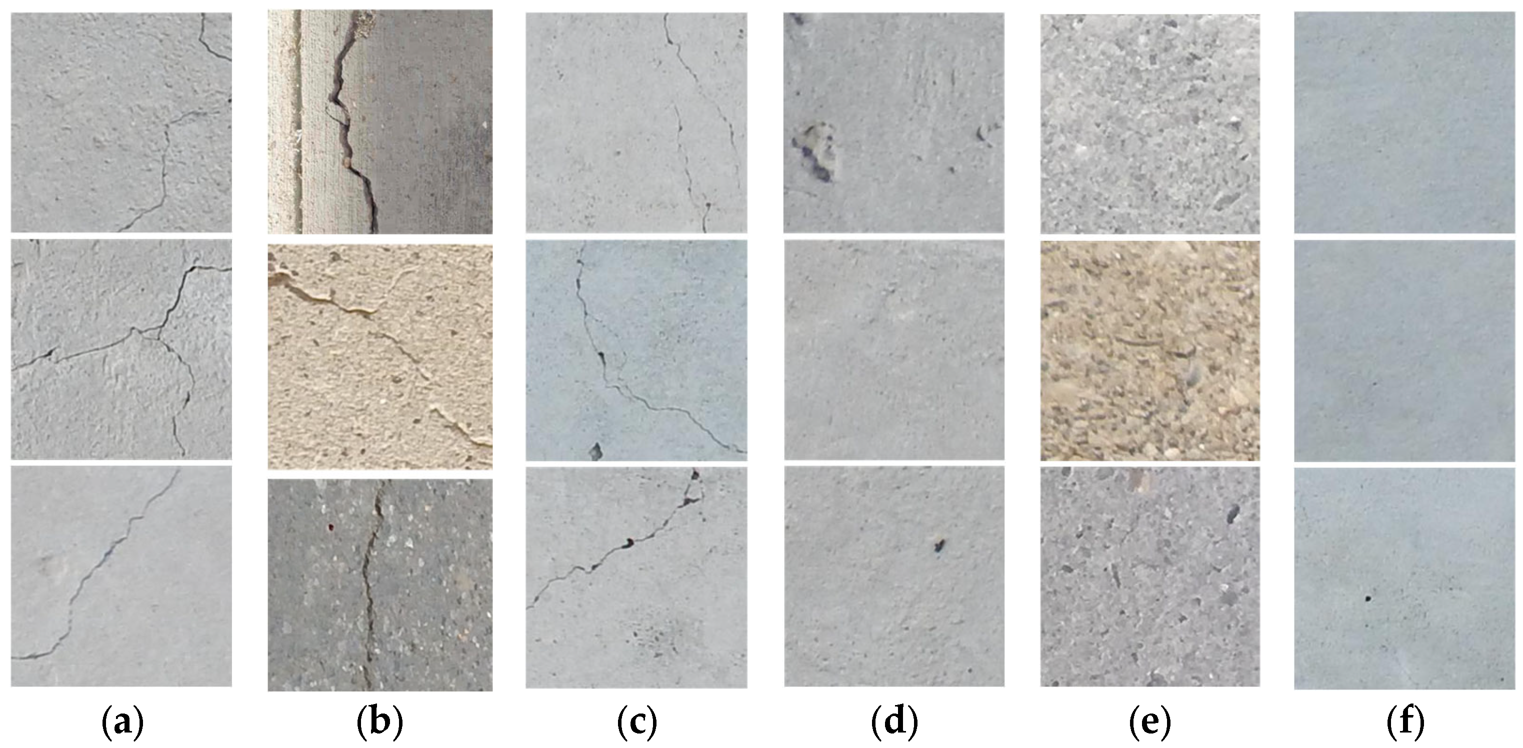
This study collected and curated a dataset comprising 106,998 images by conducting literature research, gathering data, and capturing a wide range of concrete crack images on the campus [27,28,29,30,31,32,33,34,35,36,37,38,39,40,41,42,43,44,45,46]. Among them, 40,129 images contained cracks, while 67,608 images were without cracks. To ensure the generalization of the model, the dataset includes various materials such as concrete bridge decks, parts of road surfaces, and walls within the university campus, as shown in Figure 2. These images were captured from different angles, scales, lighting conditions, and noise levels, ensuring the diversity of the dataset to enable the model to learn the wide-ranging characteristics of cracks and avoid overfitting to specific limited data [47].

2.1. Data Augmentation

The original dataset exhibits a significant class imbalance between images with cracks and images without cracks. Therefore, in this chapter, data augmentation techniques are employed to augment the dataset and enhance the model’s generalization ability. Common data augmentation methods involve random cropping, flipping, and rotation of the original data to generate additional samples, ensuring that the augmented dataset better reflects the variations and complexities in real-world scenarios, thereby increasing the data volume. By randomly applying cropping, flipping, and rotation to the original images, this chapter expands the samples based on the original data, as shown in Figure 3. The number of images in the augmented dataset, both with and without cracks, is uniformly increased to 70,000 each. The final dataset scale is expanded to 140,000 images. Subsequently, the dataset is randomly partitioned, with 80% of the samples used as the training set, 10% as the validation set, and 10% as the test set. The subsequent model training in this chapter will be conducted on this dataset to improve the CNN’s prediction accuracy and robustness to new data.

2.2. Image Grayscaling and Normalization

Due to the diverse sources and formats of the 140,000 image samples in the dataset, as well as variations in image sizes and dimensions, these issues can impact the accuracy and stability of the model. Therefore, it is necessary to perform standardized integration processing on the data, including image grayscale conversion, image normalization, and image scaling, among other image preprocessing techniques. Grayscale conversion reduces the data volume and accelerates model training speed by converting the color images into grayscale, which highlights essential information such as the edge contours of the cracks, significant for detecting concrete bridge crack diseases. Additionally, for lightweight detection algorithms, grayscale images have lower data volume and storage space compared to color images, making them more suitable for lightweight detection requirements.

Image normalization involves unifying the sizes of input images to a standardized dimension of 128 × 128 pixels. Although simple resizing can be applied to achieve the specified size, it may result in stretching distortions if the original images have different aspect ratios. Therefore, in this chapter, the images are proportionally scaled down to 128 × 128 pixels, and black padding is used to maintain the aspect ratio unchanged. This method ensures that all images are scaled to the same size without altering their aspect ratios, facilitating model training and application.

Image normalization is essential as well. The pixel values of input images are originally within the range of 0 to 255, which might be too large for CNN training. It can cause challenges in optimization algorithms based on gradients, such as slow convergence or vanishing/exploding gradients. To address these issues, image normalization is performed, rescaling the pixel values to a range between 0 and 1.

In summary, the data preprocessing techniques, including grayscale conversion, image normalization, and image scaling, are applied to the dataset to standardize and enhance its quality. These steps are crucial for improving model accuracy, stability, and convergence during CNN training for concrete bridge crack detection.

First, the image’s RGB three-channel pixel values are converted to grayscale using the weighted average method with the “cv2.IMREAD_GRAYSCALE” function from the OpenCV library, as shown in the following equation:

$$Gray(x,y)=0.299R(x,y)+0.587G(x,y)+0.114B(x,y)$$

(1)

The grayscale value Gray(x,y) is obtained by converting the RGB three-channel pixel values R(x,y), G(x,y), and B(x,y) using the weighted average method. The weighted coefficients are determined based on the human eye’s sensitivity to different colors and have been widely applied in image processing and computer vision fields [48].

Next, the images are uniformly resized to 128 × 128 while maintaining the original aspect ratio, and any remaining empty areas are filled with black pixels. Finally, the images are normalized by scaling each pixel value to the range of 0 to 1. The image preprocessing results are shown in Figure 4. However, since the pixel values are reduced to a small range of 0 to 1, the normalized images cannot accurately display the details and differences in the image.

3. Establishment of Models

3.1. Architecture of Networks

To date, CNN has been developed for several decades and has given rise to various classic architectures such as VGGNet [33], GoogleNet [49], ResNet [50], and DenseNet [51]. However, in the context of lightweight detection tasks, the parameter count of these models still appears to be excessively complex and large. Therefore, building upon the findings of the previous research [47], this study introduces a more straightforward and novel lightweight CNN architecture, as illustrated in Figure 5.

The lightweight CNN model utilizes the Adaptive Moment Estimation (Adam) [52] as the optimizer and employs binary cross-entropy as the loss function. The model consists of three sets of convolutional and pooling layers. After preprocessing, the input is a 128 × 128 image. First, it passes through the first block, comprising a convolutional layer with 16 filters of size 3 × 3, followed by a pooling layer of size 2 × 2, and then a Dropout layer. Next, it goes through the second block, consisting of a convolutional layer with 32 filters of size 3 × 3, a pooling layer of size 2 × 2, and a Dropout layer. The third block contains a convolutional layer with 32 filters of size 3 × 3, a pooling layer of size 2 × 2, and a Dropout layer. Finally, the Global Average Pooling layer and the output layer achieve the detection. $L_2$ regularization is applied to the weights of each convolutional layer.

To achieve lightweight optimization of the model and to consider the possibility of overfitting during training, various methods have been implemented, including the addition of Global Average Pooling layer, Dropout, $L_2$ regularization, and an early stopping mechanism as following:

3.1.1. Global Average Pooling (GAP) Layer

The GAP layer is essentially a pooling layer used to convert the high-dimensional feature maps obtained from the convolutional layers into a one-dimensional vector. In typical CNN classification networks, Flatten and Dense layers are used for dimensionality reduction and mapping of data. However, Dense layers contain a large number of parameters, which often contribute significantly to the total parameter count of the CNN. To ensure that the final CNN model meets the requirements of lightweight design, the GAP layer is used instead of Dense layers to achieve data dimensionality reduction, thereby avoiding excessive parameters and reducing the risk of overfitting.

3.1.2. Dropout Method

Dropout is a common regularization technique used to prevent overfitting in CNNs and reduce the number of parameters in the model. During training, Dropout randomly sets a certain proportion of node outputs to zero, effectively removing some nodes from the network. This creates different sub-networks during each training iteration, effectively serving as an ensemble learning method. During testing, Dropout does not perform random node removal but multiplies all node outputs by a retention probability. This forces the network to learn different features and suppress specific neurons, thereby enhancing the network’s robustness. Typically, Dropout probability is set between 0.2 and 0.5, and the specific value will be determined during the subsequent hyperparameter optimization.

3.1.3. L₂ Regularization

Another way to limit the size and number of model parameters and reduce overfitting is by adding a penalty term to the model’s loss function. $L_2$ regularization, as a commonly used regularization method, adds a regularization term to the neural network’s loss function, which is equal to the sum of squares of all weights multiplied by a regularization coefficient [53]. During model training, $L_2$ regularization encourages weights to shift towards smaller values, preventing some features from having an overly large impact on the results and reducing the risk of overfitting. The formula for $L_2$ regularization is as follows:

$$L_2={\displaystyle \frac{\lambda }{2}}\sum _{i=1}^n{\omega }_i^2$$

(2)

where $\lambda$ represents the regularization coefficient, $n$ is the number of elements in the weight matrix, and ${\omega }_i$ denotes the $i$-th element of the weight matrix. The regularization coefficient $\lambda$ will be determined in the next section during the hyperparameter optimization process.

3.1.4. Adding Early Stopping Mechanism

The early stopping mechanism is an effective method to prevent overfitting. It monitors the loss function value on the validation set during the training process to decide when to stop training and avoid overfitting. As mentioned in the previous section, the dataset is divided into training, validation, and testing sets. A key sign of overfitting is when the loss function value keeps decreasing on the training set but increases on the validation and testing sets. This indicates a potential issue with the model’s generalization performance, known as overfitting. The early stopping mechanism aims to prevent overfitting by monitoring the loss function value on the validation set during training. If the loss value on the validation set does not decrease for a continuous number of epochs (specified as the early stopping coefficient, in this case set to 5), the training process will be stopped prematurely.

3.2. Optimization of Hyperparameters

Hyperparameters are parameters that need to be manually specified when training a neural network. They determine the model’s structure and optimization process, such as the optimization algorithm, learning rate, dropout probability, regularization coefficient, etc. Unlike model parameters like weights and biases, hyperparameters cannot be learned during the training process and have a significant impact on the model’s performance. A set of well-chosen hyperparameter values can greatly improve the model’s performance and efficiency, especially in lightweight tasks, where optimal hyperparameter combinations can make the CNN model effectively utilize limited computational resources. Therefore, hyperparameter optimization for the CNN model is crucial before conducting model training.

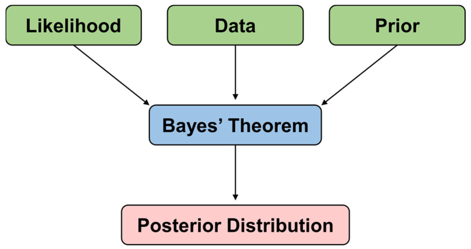
The most commonly used methods for hyperparameter tuning are manual search, grid search, random search, and Bayesian optimization. Manual search is the simplest method, where different hyperparameter combinations are tried manually. However, this method is highly inefficient, especially when dealing with a large number of hyperparameters, and it may not find the optimal solution. Grid search exhaustively enumerates all possible hyperparameter combinations to find the best one. However, it is computationally expensive, and as the number of parameters increases, the number of combinations to be evaluated grows exponentially. Random search is more efficient than grid search as it randomly selects a certain number of hyperparameter combinations for evaluation, but it cannot guarantee finding the global optimal solution. On the other hand, Bayesian optimization is an advanced method for hyperparameter tuning. It uses Bayesian updating to update the confidence in the objective function, iteratively choosing the most likely hyperparameter combinations that are expected to improve the model’s performance. Bayesian optimization can find the optimal hyperparameter combination with fewer evaluations. Therefore, in this paper, we adopt Bayesian optimization for hyperparameter tuning, as shown in Figure 6.

Four hyperparameters have been selected for optimization, which are the activation function, learning rate, Dropout probability, and $L_2$ regularization coefficient.

The activation function is a non-linear function used to introduce non-linearity into the neural network. Without activation functions, the convolutional and fully connected layers would be equivalent to linear mappings from input to output. Activation functions allow the network to learn non-linear mappings, enabling the model to handle non-linear problems, increasing the model’s capacity for fitting, and performing tasks such as non-linear classification and regression.

As shown in Figure 7, four common activation functions are selected for tuning:

The Sigmoid function, one of the earliest activation functions, maps any real number input to the range. Its formula is:

$$f_{Sigmoid}(x)={\displaystyle \frac{1}{1+e^{-x}}}$$

(3)

where $x$ is the input to the function, and $e$ is the base of the natural logarithm (approximately equal to 2.71828). As $x$ approaches positive infinity, $f\left(x\right)$ approaches 1, and as $x$ approaches negative infinity, $f\left(x\right)$ approaches 0. While its output range is useful for binary classification by representing probabilities, Sigmoid suffers from the vanishing gradient problem. This issue significantly hinders training deep neural networks by causing slow convergence and updating difficulties. Consequently, other activation functions, notably ReLU and its variants, have gained popularity.

The Tanh function is similar to the Sigmoid function, but it maps the input to the range [−1, 1]. The formula for the Tanh function is:

$$f_{Tanh}(x)={\displaystyle \frac{e^x-e^{-x}}{e^x+e^{-x}}}$$

(4)

where $x$ is the input to the function, and $e$ is the base of the natural logarithm. Tanh’s symmetric, zero-centered output provides an advantage over Sigmoid by potentially reducing the vanishing gradient problem, making it generally more suitable for deep neural networks. However, like Sigmoid, Tanh can still suffer from vanishing gradients for extreme input values. While used in hidden layers, it is less frequently applied than ReLU and its variants in modern CNNs, as ReLU has proven more effective in mitigating vanishing gradients and accelerating training.

ReLU, which stands for Rectified Linear Unit, is currently one of the most popular activation functions in deep learning. It is a simple and efficient activation function that has strong advantages in various applications and helps address the vanishing gradient problem. The ReLU function is defined as:

$$f_{Relu}\left(x\right)=\mathrm{m}\mathrm{a}\mathrm{x}(0,x)$$

(5)

In other words, it returns the input $x$ if it is positive or zero, and returns zero if the input is negative. This piecewise linear function introduces non-linearity to the neural network, allowing it to learn complex patterns and relationships in the data.

One of the key advantages of ReLU is that it does not suffer from the vanishing gradient problem, which can occur with other activation functions like Sigmoid and Tanh. The vanishing gradient problem can cause the gradients to become extremely small during training, leading to slow convergence and difficulty in updating the model’s parameters effectively. ReLU’s derivative is either 1 (for positive inputs) or 0 (for negative inputs), which means the gradient remains constant and does not vanish as the input increases, making it easier to train deep neural networks.

Softmax function is commonly used in multi-class classification problems. It is used to convert the output scores of a neural network into probability values that lie in the range [0, 1] and ensure that the sum of all probabilities is equal to 1, representing the probabilities of each class:

$$f_{Softmax}(x)={\displaystyle \frac{e^x}{\sum e^x}}$$

(6)

Softmax is crucial for obtaining probability distributions over classes and is essential in training models to minimize the difference between predicted probabilities and true labels. However, it is sensitive to input score magnitudes, potentially leading to numerical instability. The “Log-sum-exp trick”, involving subtracting the maximum score before application, is a common practice to stabilize computation.

The learning rate controls the magnitude of updates in the gradient descent algorithm. Its size directly affects the training speed and performance of the model. If the learning rate is too small, the convergence speed of the model will be very slow, and it may require more iterations to reach the optimal solution. On the other hand, if the learning rate is too large, each update may skip the optimal solution, leading to the model being unable to converge or even diverge. The optimal hyperparameter combination was determined through Bayesian optimization, as shown in

Table 1. Optimal hyperparameter combination.

Activation Function	Learning Rate	Dropout	L2 Regularization Coefficient
ReLU	0.001	0.3	0.001

.

4. Visualization of Detection Results Based on Image Stitching

Image stitching is the process of combining two or more images with overlapping regions to create a panoramic image. Image stitching algorithms are one of the oldest and most widely used techniques in the field of computer vision [54,55].

In bridge inspection, a single image often fails to reveal the complete view of cracks and provide a comprehensive overview. However, through the use of image stitching techniques, engineers can quickly obtain high-resolution panoramic images of the entire bridge deck and sides, allowing them to understand the development of cracks and other defects. Compared to traditional bridge inspection methods that rely on bridge inspection vehicles and manual visual inspection, using UAVs for image acquisition and subsequent image stitching enables the display of panoramic images covering the entire inspection area, greatly enhancing safety, efficiency, and cost-effectiveness. Finally, by combining the image stitching results with the crack detection algorithms mentioned earlier, accurate and detailed records can be generated, effectively digitizing and illustrating the inspection findings, providing visually accessible inspection results.

4.1. Image Preprocessing

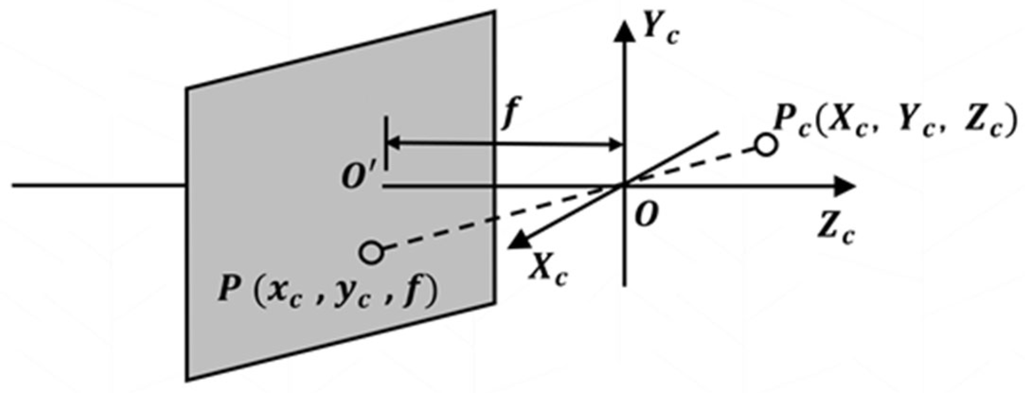
The imaging process of a camera can be summarized as projecting a point in the world coordinate system onto a point on the camera imaging plane. In the three-dimensional space, there exists a multi-view geometric relationship between features in the world and their corresponding projected features on the imaging plane. This process can be represented as a homogeneous transformation, which is expressed as the camera projection matrix [56]. The camera imaging model is shown in Figure 8, where $Z_c$ represents the optical axis, $O^{\prime }$ is the intersection point of the imaging plane and the optical axis, and ${OO}^{\prime }$ is the focal length $f$. However, before performing image stitching, camera imaging may encounter camera distortion, and uneven lighting under the bridge may affect the image quality. Therefore, it is necessary to preprocess the input images by performing camera distortion correction and lighting correction to ensure the stitching result’s accuracy and quality.

4.1.1. Camera Distortion Correction

Camera distortion refers to the noticeable radial and tangential distortions that occur during the imaging process, particularly with wide-angle lenses. These distortions cause straight lines to appear curved in the image projection, potentially leading to changes in shape and size within the image. Consequently, accurate feature matching may be compromised, resulting in blurred effects in the stitched image and affecting the final panorama stitching outcome. To address the radial and tangential distortions introduced by camera imaging, a quadratic distortion model is commonly employed for correction. Given a pixel point ($x_c,y_c$), the coordinates after distortion correction are denoted as ($x_c\prime ,y_c\prime$). Radial distortion modeling can be conducted by the following equations:

$$x_c^{\prime }=x_c+∆x_c=x_c+k_1{r}^2+k_2{r}^4$$

(7)

$$y_c^{\prime }=y_c+∆y_c=y_c+k_3{r}^2+k_4{r}^4$$

(8)

where ($k_1, k_2, { k}_3, k_4$) are radial distortion coefficients, and $r$ represents the distance of the pixel point to the camera’s optical center (also known as the camera’s principal point or image center). Tangential distortion modeling can be conducted by the following equations:

$$x_c^{\prime }=x_c+∆x_c=x_c+\left[2p_1{y}_c+p_2\left(r^2+2x_c^2\right)\right]$$

(9)

$$y_c^{\prime }=y_c+∆y_c=y_c+\left[p_1\left(r^2+2y_c^2\right)+2p_2{x}_c\right]$$

(10)

where the tangential distortion coefficients ($p_1, p_2$) are another type of distortion caused by the camera lens, which results in the bending of straight lines in both horizontal and vertical directions. Similarly to radial distortion, tangential distortion also needs to be corrected to improve the accuracy and precision of the images.

4.1.2. Lighting Correction

During the process of image acquisition of bridges using UAVs or other methods, the images collected may be affected by various factors such as human operations and variations in outdoor lighting, resulting in discrepancies in brightness, contrast, and color compared to the actual scene. Such errors could have adverse effects on the extraction and registration of feature points during the subsequent image stitching process.

To address this issue, hardware solutions may involve using flashlights or supplementary lighting during image capture to compensate for insufficient natural light. However, using flashlights while capturing images of bridge cracks, seepage, and corrosion could lead to undesired reflections and glare, further affecting the subsequent stitching and recognition process. Additionally, flashlights have limited illumination range, and achieving satisfactory lighting results for high-altitude areas such as the sides and undersides of bridges might be uneconomical and pose safety concerns.

In the software domain, several methods have been developed for light correction: Bilateral filtering is a non-linear filtering technique that smoothens an input image while considering the spatial and grayscale distribution of pixels. By preserving edge information and suppressing noise, bilateral filtering can effectively achieve light correction [57]. However, the complexity of its parameters makes it difficult to adjust, often requiring substantial tuning, which poses high hardware requirements. Moreover, the filtered image may still suffer from blurring, impacting image clarity and potentially compromising the accuracy of crack detection.

Gaussian mixture models assume that each pixel is a mixture of independent lighting components and materials, and the image can be modeled as a mixture of these components. By fitting the model to the color distributions of source and target images, each pixel in the source image can be mapped to the corresponding pixel in the target image based on probabilities. This method can handle complex lighting variations while preserving local details [58]. However, it may perform poorly in regions with significant lighting differences, and the estimation of model parameters, such as means and covariances, may require considerable computational resources and may affect the correction effectiveness for high-quality images with numerous pixels.

The multi-scale Retinex algorithm is a typical image enhancement method derived from the original Retinex algorithm. The Retinex algorithm is a color constancy method that enhances contrast by applying a logarithmic transformation to the image. In contrast, the multi-scale Retinex algorithm combines multiple scales of the Retinex algorithm using multiple Gaussian filters with different ratios to separate the illumination and reflection components of the image. These components are then combined with different weights, optimized to achieve improved contrast and color balance, thereby adapting better to images captured under different lighting conditions [59]. However, this method requires strict parameter selection and may not be suitable for highlighting high-light or low-light areas in images, leading to over-enhanced results.

Deep learning methods have emerged as a novel approach to light correction in recent years, owing to rapid advancements in computer vision [60]. Typically, these methods involve training a neural network to enhance images affected by poor lighting, thereby achieving light correction. Based on the trained model, these methods exhibit high robustness and can effectively correct images under various lighting conditions. However, they also face challenges in terms of computational resources, as training the model requires a substantial amount of training data and hardware capabilities. Achieving a well-trained model may also demand a significant training time, and inadequate computational resources can compromise the model’s generalization ability and the accuracy of correction results.

Histogram equalization is one of the most common light correction methods employed in practical applications. It enhances the global contrast and dynamic range of an image by remapping the grayscale image. It yields the best results when the available data in the image is represented by tight contrast values. For instance, in the medical field, histogram equalization can better display skeletal structures in X-ray images and reveal more details in other overexposed or underexposed photos [61]. The key advantage of this method lies in its relative simplicity, as it does not place excessive demands on computing devices and resources. Hence, it is well-suited for implementation in this paper across various detection methods, and it effectively highlights cracks by enhancing contrast.

In this paper, histogram equalization is adopted for light correction to enhance images. The process involves converting the image from the BGR color space to the LAB color space and applying histogram equalization to the brightness channel (L channel). The output result is then combined with the original green-red axis (A channel) and blue-yellow axis (B channel) before converting the LAB image back to the BGR image for output. Figure 9 illustrates the results of the light correction experiment (see red box in Figure 9a), demonstrating significant enhancement of image details, particularly in crack detection, where the edges and contours of cracks are well highlighted.

4.2. Feature Detection

Feature detection is a crucial step in the image stitching process as it greatly influences the accuracy of subsequent image matching and, consequently, the final result of image stitching. Each image contains key local features that are typically referred to as “keypoint features”, “interest points”, or “corners”. These features are described based on the performance of pixel blocks around their locations. In the context of crack detection, the edges and contours of cracks represent typical “edge features”. These feature points possess good invariance and distinctiveness, allowing for matching different types of features based on their orientations and local representations. Consequently, they can identify corresponding regions in different images for stitching and serve as ideal indicators even when object boundaries and occlusions are present in the image sequence [62].

Currently, common feature detectors include the Scale Invariant Feature Transform (SIFT) algorithm [63], Speeded Up Robust Features (SURF) algorithm [64], and Oriented FAST and ORB [65]. The latter two are variants of the SIFT algorithm. Here is a brief introduction to these three algorithms:

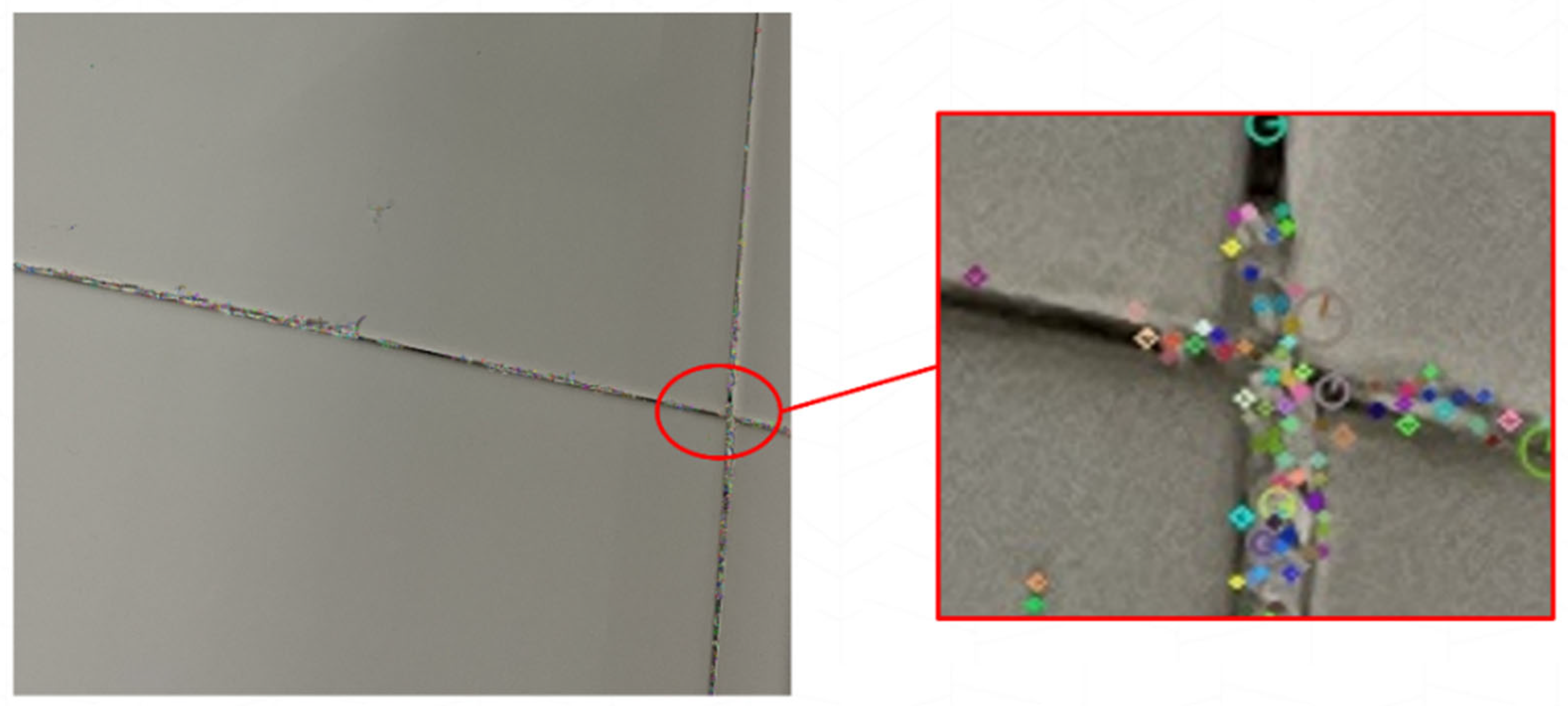
The SIFT algorithm analyses the Gaussian pyramid level of each point and computes the feature points by calculating the gradient magnitude and orientation of each pixel in a 16 × 16 window around the keypoint. To account for the influence of inaccuracies in position, it employs Gaussian weighting. In Figure 10, an example of a 16 × 16 pixel block and a 2 × 2 descriptor array is shown. The red circle in Figure 10a represents the Gaussian weighting, and Figure 10b illustrates the use of trilinear interpolation to calculate the weighted gradient orientation histogram within each subregion. The SIFT algorithm uses a Gaussian difference pyramid to determine the scale space, enabling the detection of the same feature in images with different scales. It also calculates the gradient direction of the feature point to ensure the descriptor’s orientation remains invariant during image matching with rotation, as shown in Figure 11, where the different scales of the feature points are represented by circles of varying sizes, and the lines within the circles indicate the main orientation of each feature point.

The SURF algorithm has a similar principle to SIFT, but it uses Haar wavelet transform in each subregion instead of the Gaussian convolution used by SIFT to accelerate the computation of horizontal and vertical responses. These responses are accumulated into a 64-dimensional vector as the feature descriptor, while SIFT’s feature descriptor is 128-dimensional. The SURF algorithm has a faster response speed than SIFT, but its accuracy is lower, making it unsuitable for high-precision applications.

The ORB algorithm combines the Oriented FAST and Rotated BRIEF methods to improve the rotation invariance and computational efficiency of feature points [66]. It is based on the FAST corner detection algorithm, which identifies and detects feature points based on the intensity of the surrounding regions. It performs keypoint detection at multiple scales and orientations on different levels of the image pyramid and uses the Harris response function to filter corner points. Then, it employs the BRIEF method to generate binary descriptors, resulting in a 256-dimensional feature descriptor. The ORB algorithm’s response speed is usually faster than SURF and SIFT because it uses binary feature descriptors, which require fewer computations compared to the floating-point feature descriptors used in SURF and SIFT. However, its performance is not as good as SIFT when dealing with high-precision tasks.

In summary, SIFT can effectively overcome disturbances in images, such as translation, scaling, rotation, and noise, making it robust. Compared to SURF and ORB algorithms, SIFT is more suitable for tasks that require high precision in object recognition and image matching. It can adapt well to the subsequent stitching and recognition of cracks in this study. Therefore, SIFT is chosen as the feature detection algorithm in this research, and the detected feature points are marked with circles, as shown in Figure 12.

4.3. Image Registration

After detecting and extracting the feature points in the images to be stitched, to accurately stitch multiple images, it is necessary to establish the corresponding relationships between these features in each image. Image registration is the process of verifying whether the matched features in different views or at different times are geometrically consistent, and then mapping them to the same coordinate system through geometric transformations for alignment. In image stitching, image registration is a challenging and critical step that significantly affects the final stitching result. Currently, there are two common methods for image stitching: direct registration and feature-based registration.

4.3.1. Direct Registration

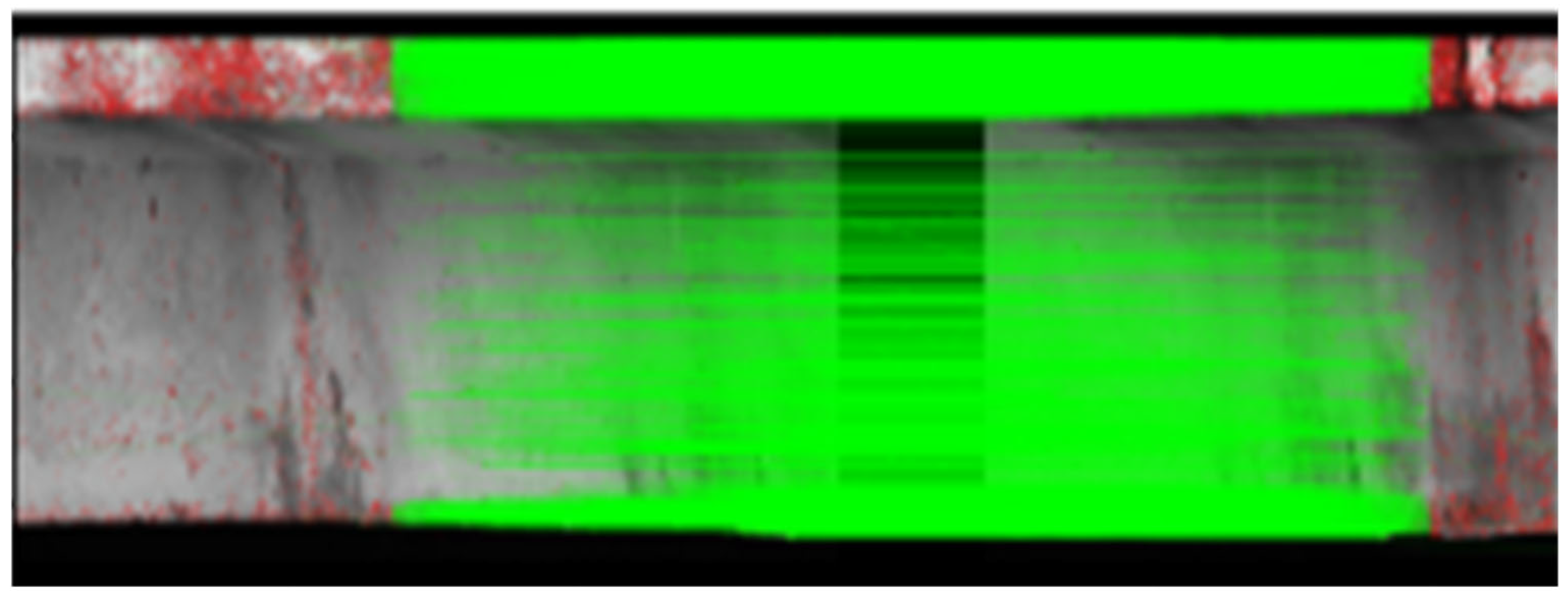
Pixel-level comparison-based registration method is the simplest and most fundamental approach for image registration. It involves directly comparing the grayscale values of pixels between images to determine the transformation relationship and then proceed with the registration. Theoretically, this method can utilize multi-layer image pyramids with a coarse-to-fine framework to reduce computational complexity and improve accuracy [67]. However, in practical applications, this method has limited convergence range, and using image pyramids with more than three layers can lead to significant loss of image details, which contradicts the high precision requirement in this study. Moreover, the robustness of direct registration is relatively poor, making it susceptible to interference from environmental factors such as lighting and noise. It often yields unsatisfactory results when dealing with images with only a small overlap or significant contrast variations. As shown in Figure 13, direct registration was applied to stitch images of a real bridge on campus, resulting in noticeable stitching seams on the left and severe misalignment and ghosting on the right. Therefore, an alternative registration method is needed to address these issues.

4.3.2. Feature-Based Registration

Image feature point distribution is often uneven, and early feature-based matching methods typically rely on simple relationships between feature points and their surrounding pixel blocks for matching. However, this approach may not perform well when dealing with image rotations and other transformations. Currently, feature-based registration methods have evolved to possess strong robustness and can handle recognition of known objects under significant viewpoint variations [63]. They can produce responses for strong corners [68], blob-like regions [63], and uniform areas [69]. Moreover, feature detection algorithms can extract the main orientation of feature points at different scales, enabling accurate registration of images with different sizes, scales, rotations, or occlusions. They also exhibit strong robustness against environmental factors such as lighting variations, oil stains, and scratches.

Approximate Nearest Neighbor (ANN) Matching

The Approximate Nearest Neighbor (ANN) matching is a fast algorithm for searching the nearest neighbors [70]. It involves constructing specific data search structures, such as k-d trees, Locality-Sensitive Hashing (LSH), and Fast Library for Approximate Nearest Neighbors (FLANN). Then, it calculates the Euclidean distance between detected feature points in the images to determine the matching points with the smallest Euclidean distance. Among the data structures, k-d trees are commonly used, as they are binary trees for spatial partitioning. The data points are divided into left and right subsets within the k-d tree, and this process is repeated until each subset contains only one point. During the search, it starts from the root node and traverses down the left or right subtree until reaching a leaf node. Finally, it backtracks from the leaf node and calculates the distance from each node to the input point, selecting the minimum distance.

The ANN matching method utilizes prebuilt data search structures, allowing for fast searching of nearest neighbors. It is efficient regardless of the size of the dataset and requires relatively small storage space, making it suitable for processing large-scale datasets. However, the points found by the ANN matching method are not true matching pairs in a strict sense, as it may produce many matching errors in practical applications. When the number of erroneous matching pairs exceeds a certain threshold, it can lead to blurriness or even errors in the image stitching. Due to this limitation, it is necessary to find a more accurate matching algorithm.

Random Sample Consensus (RANSAC) Algorithm

In cases where the noise in the image does not follow a normal Gaussian distribution, conventional methods like least squares and M-estimation [71] may suffer from decreased performance because some gradient descent algorithms may fail to converge to the global optimum. To address this issue, Michael Fischler and Robert Bolles proposed a parameter estimation method called the RANSAC algorithm [72], which can estimate model parameters from noisy data and resist the interference of certain non-Gaussian noise.

The RANSAC algorithm first selects k corresponding subsets, calculates the initial estimate p, and then computes the residual of the full set of corresponding points:

$$r_i=‖x_i\prime \left(x_i;p\right)-{\tilde{x}}_i\prime ‖$$

(11)

where ${\tilde{x}}_i\prime$ represents the estimated position, and $x_i\prime$ represents the detected position of the feature points. Subsequently, the number of inliers is calculated, which refers to the points within a predicted distance $\epsilon$ (typically one to three pixels), denoted as $‖r_i‖\le \epsilon$. The computation of the minimum median variance involves calculating the error between each data point and the fitting model, followed by selecting the minimum of ${‖r_i‖}^2$, and then computing the median of these values as the model error. The random selection process is repeated $S$ times, and the sample set containing the most inliers or having the smallest median residual is considered the final solution. The initial parameters $p$ or the computed inlier set are passed to the next step of data fitting, where iterative refinement is performed to obtain a set of parameters that provide the most optimal fitting result. Figure 14 illustrates an example of feature point matching obtained through the RANSAC algorithm, and the complete stitching effect will be presented in the next section.

The RANSAC algorithm employs random sampling, which enables it to effectively handle noise, outliers, and other interfering data, yielding reliable models with robustness and accuracy. Moreover, it does not rely on prior knowledge and can automatically discover models that meet the specified criteria from the data. Therefore, this method is highly suitable for the image stitching algorithm in this study. Subsequently, the RANSAC algorithm will be used to compute transformation matrices based on matched point pairs, facilitating the registration and alignment of the images to be stitched together.

5. Test and Results Analysis

5.1. Model Training

In this section, the dataset containing 140,000 images will be partitioned into training, validation, and test sets in an 8:1:1 ratio. The constructed CNN model will be trained using the following software environment and hardware facilities, as shown in

Table 2. Software environment.

Compile Software	Python	TensorFlow	Keras	CDUA	CuDNN
PyCharm	3.9	2.6.0	2.6.0	11.2.0	8.1.0

and

Table 3. Hardware equipment.

Operating System	CPU	GPU	Memory
Windows 10	Intel® Xeon® W-2255	NVIDIA GeForce RTX 3090	DDR4 64 GB

.

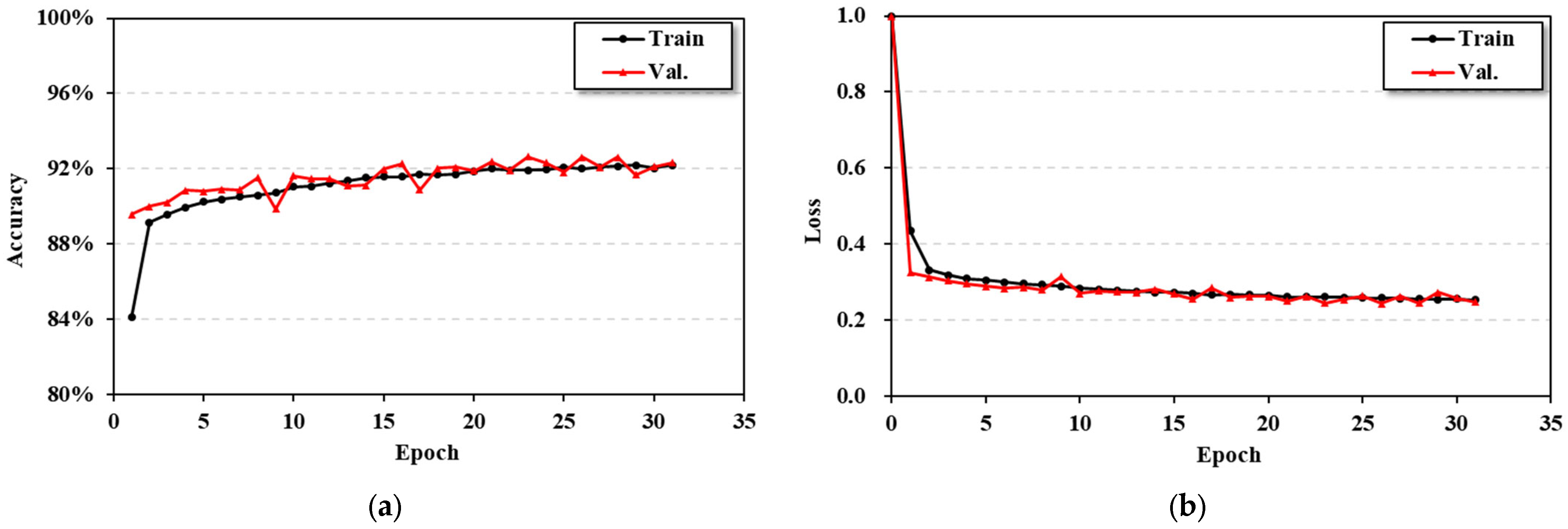
To provide a visual understanding of the model training process, this chapter utilizes the TensorBoard tool to record training logs and visualize the training in real-time, continuously monitoring the model’s performance. Figure 15 shows the variations in Accuracy and Loss during the model training.

After 31 epochs of training CNN (with a batch size of 64), the training process automatically stopped due to early stopping intervention, as the Accuracy and Loss on the validation set tended to converge. The final model achieved an accuracy of 92.2% and a loss value of 0.253 on the training set, while on the validation set, it achieved an accuracy of 92.3% and a loss value of 0.248.

5.2. Index of Performance of Models

To comprehensively evaluate the performance of the trained CNN model, four evaluation metrics were used on the completed model: Confusion matrix, Test accuracy, Recall, and F1-score.

As mentioned earlier, the dataset was divided into training set (80%), validation set (10%), and test set (10%). The training set was used to train the model, the validation set was utilized for hyperparameter tuning and monitoring the training process, and the test set was used to assess the model’s generalization performance. All four evaluation metrics were calculated on the test set, which consists of 14,000 samples.

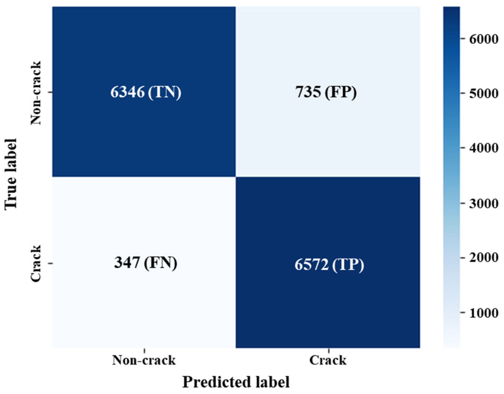
The Confusion matrix is a visualization matrix used to analyze the model’s performance. It compares the model’s predicted results with the true labels to compute the number of correct and incorrect predictions. The Confusion matrix for the model in this chapter is shown in Figure 16. It includes the following components:

• True Negative (TN): The number of samples predicted as negative and are actually negative.
• True Positive (TP): The number of samples predicted as positive and are actually positive.
• False Negative (FN): The number of samples predicted as negative but are actually positive.
• False Positive (FP): The number of samples predicted as positive but are actually negative.

By analyzing the Confusion matrix, we can observe that the test set contains 14,000 randomly selected samples. Among these, 7081 samples are without cracks (6346 true negative and 735 false positive), and 6919 samples are with cracks (6572 true positive and 347 false negative). The test set’s positive-to-negative sample ratio is similar to that of the entire dataset, ensuring an accurate evaluation of the model’s performance.

The results from the Confusion matrix indicate that the CNN model’s overall predictive performance is good. It correctly predicts 6346 samples without cracks and 6572 samples with cracks, suggesting that the model performs better on images with cracks compared to images without cracks.

The accuracy rate, recall rate and F1 score can all be obtained through the confusion matrix, and the definition formula of the test set accuracy rate is as follows:

$$\mathrm{A}\mathrm{C}={\displaystyle \frac{\mathrm{T}\mathrm{P}+\mathrm{T}\mathrm{N}}{\mathrm{T}\mathrm{P}+\mathrm{T}\mathrm{N}+\mathrm{F}\mathrm{P}+\mathrm{F}\mathrm{N}}}$$

(12)

Recall is an important evaluation metric that can evaluate whether the model can correctly identify all real positive examples:

$$\mathrm{R}\mathrm{E}={\displaystyle \frac{\mathrm{T}\mathrm{P}}{\mathrm{T}\mathrm{P}+\mathrm{F}\mathrm{N}}}$$

(13)

The F1 score is a comprehensive evaluation index that can more comprehensively evaluate the performance of the classification model:

$$\mathrm{F}1=2{\displaystyle \frac{\mathrm{R}\mathrm{E}\left(\frac{\mathrm{T}\mathrm{P}}{\mathrm{T}\mathrm{P}+\mathrm{F}\mathrm{P}}\right)}{\mathrm{R}\mathrm{E}+\left(\frac{\mathrm{T}\mathrm{P}}{\mathrm{T}\mathrm{P}+\mathrm{F}\mathrm{P}}\right)}}$$

(14)

The final results are shown in

Table 4. Quantitative evaluation results of the trained model.

Accuracy Rate	Recall	F1 Score
92.27%	94.98%	92.39%

, indicating that the CNN model established in this chapter has high accuracy and recall rates. It also exhibits a high F1 score, which enables accurate detection of cracks on the concrete surface, fulfilling the fundamental requirements of the proposed lightweight detection approach.

5.3. Model Qualitative Evaluation

To further understand the model’s performance in real-world scenarios and specifically evaluate the CNN model’s lightweight detection performance on ordinary devices, a qualitative evaluation of the model was conducted. The running device was a lightweight notebook computer with specific numerical values shown in

Table 5. Laptop hardware conditions.

Operating System	CPU	GPU	Memory
Windows 11	AMD R7-4800H	Integrated graphics	DDR4 16 GB

. As the notebook does not have a dedicated graphics card but rather an integrated graphics processor within the CPU, its image processing performance is relatively weak, making it highly suitable for the lightweight detection evaluation experiments in this study.

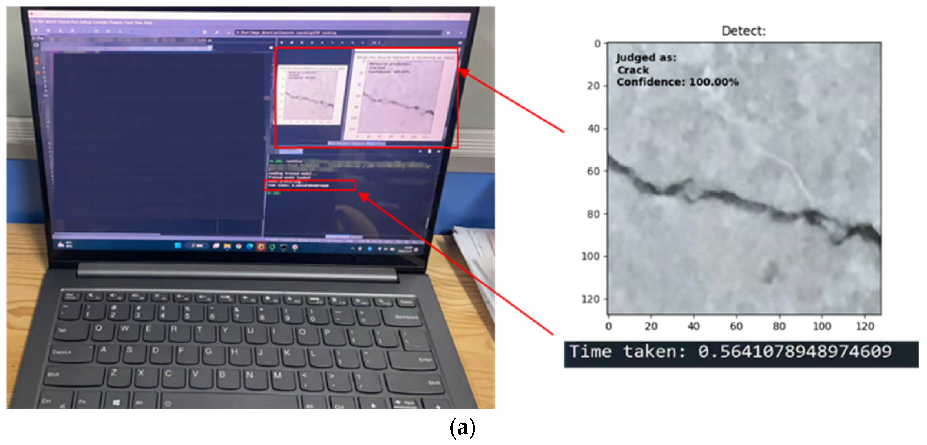
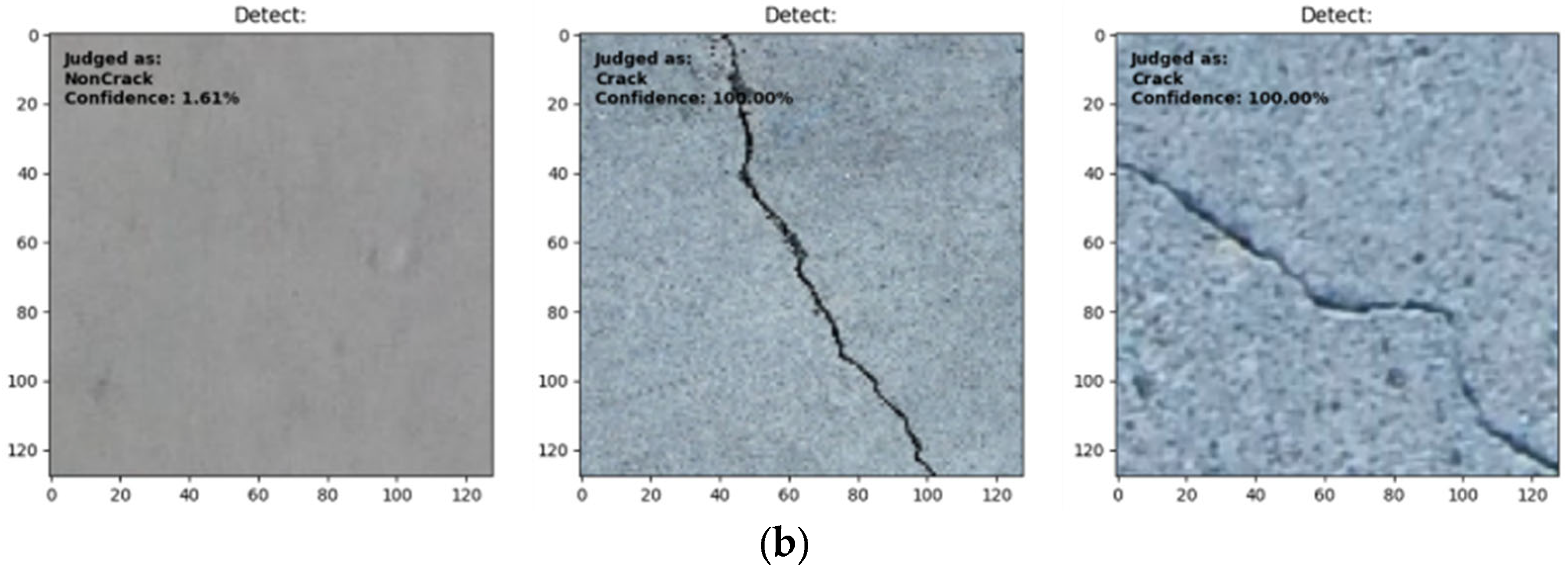
Tests have shown that the CNN model can run smoothly on a thin and light office laptop with integrated graphics, and can quickly and accurately identify and characterize the input concrete crack image within 0.564 s, as shown in Figure 17.

The above results indicate that the proosed lightweight CNN model constructed in this chapter can rapidly and accurately identify concrete bridge crack defects in a detection environment with limited computational resources and insufficient hardware equipment, meeting the engineering practical requirements for lightweight detection.

5.4. Image Stitching Test

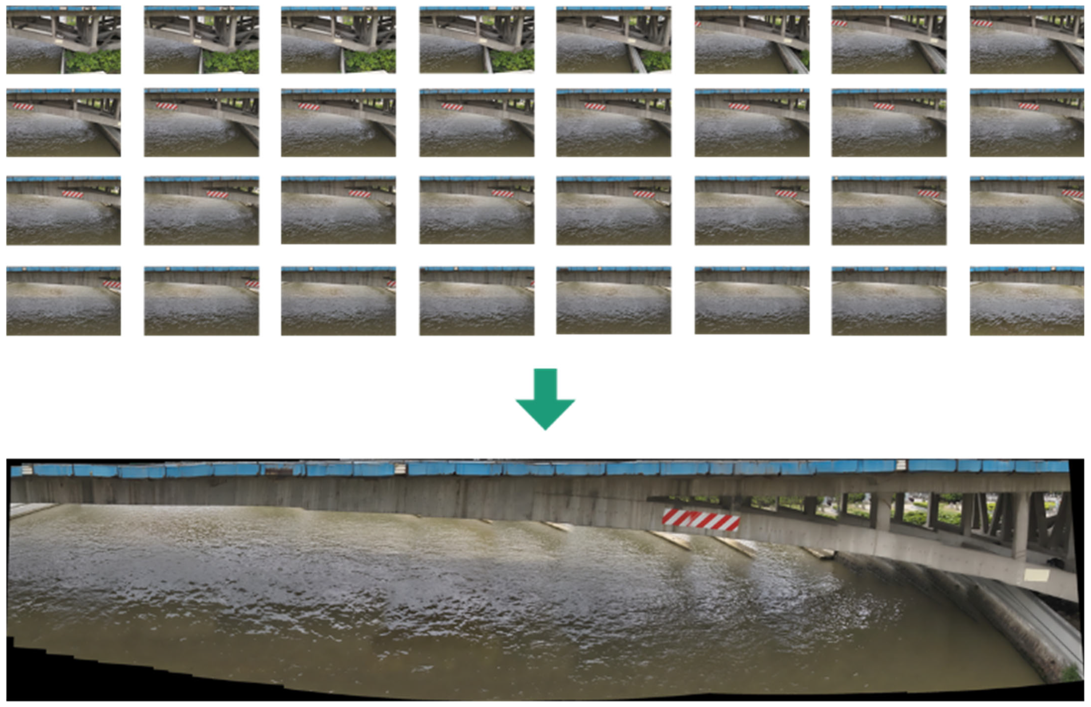
The proposed algorithm in this paper first preprocesses the input images by performing camera distortion correction and illumination enhancement using histogram equalization. Next, it utilizes the SIFT algorithm to detect and extract key feature points from the processed images to identify corresponding regions in the images. Then, the RANSAC algorithm is employed to match these feature points across all images, compute transformation matrices for each pair of adjacent images, establish correspondence, and perform alignment and transformation. Finally, the transformed images are fused together to create a panoramic image.

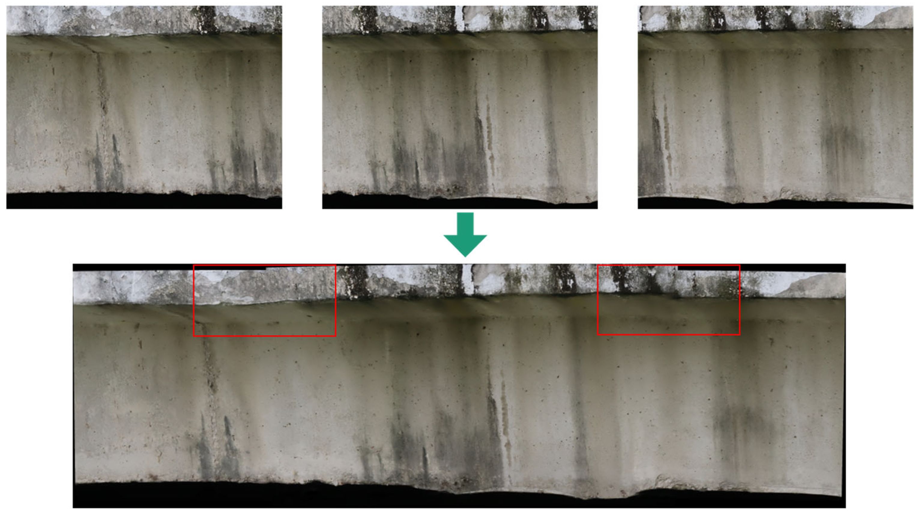
To validate the effectiveness of the algorithm, the paper conducts image stitching experiments on the side view of an existing arch bridge in Suzhou, China, as shown in Figure 18. The image stitching algorithm developed in this chapter can effectively eliminate noise and abnormal effects caused by lighting conditions, enabling rapid stitching of multiple images captured in an outdoor environment. However, it was observed in practical applications that the flow of the river under the bridge significantly affected the stitching process. The flowing water led to varying river features in each image, resulting in partial misalignment and blurriness in the stitched images for the river and the bridge area close to it.

6. Conclusions

This study successfully leveraged computer vision technology to develop an efficient and lightweight CNN for concrete surface crack detection in bridges, specifically targeting the practical needs of small and medium-sized structures with limited computational resources. Our comprehensive methodology commenced with the construction of a large-scale database of 106,998 concrete crack images, which was subsequently augmented to 140,000 images, forming a robust foundation for deep learning.

A key achievement is the development of a lightweight CNN specifically engineered for concrete crack detection. This model achieved high performance metrics on our test dataset, demonstrating a 92.27% accuracy, 94.98% recall, and a 92.39% F1 score. Crucially, the model’s lightweight design enables smooth operation and fast inference (approximately 0.564 s per image) even on standard office notebooks without requiring dedicated GPUs, making it highly suitable for real-world field inspections.

Complementing the detection, an advanced image stitching algorithm was developed to generate high-quality panoramic views of bridges from multiple images. This algorithm exhibited remarkable robustness and accuracy, effectively stitching images without visible seams, even for challenging infrared images. By integrating the crack detection results onto these panoramic views, our system provides a comprehensive and intuitive 2D visualization of detected cracks, transforming inspection data into an accessible, image-based information model for bridge maintenance and assessment.

In conclusion, this paper proposes a lightweight detection method for concrete bridge cracks based on computer vision technology, which solves the detection needs of small and medium-sized bridges from the perspective of qualitative classification. In addition, this study incorporates an image stitching algorithm to achieve two-dimensional visualization of detection results and provide an image-based information model of local components.

Despite these advancements, our study encountered some limitations during the image stitching process. Specifically, the dynamic nature of flowing water under bridges in outdoor environments led to challenges in image stitching, occasionally resulting in partial misalignment and blurriness in affected areas. Future research will focus on developing more robust stitching algorithms capable of handling dynamic backgrounds more effectively. Additionally, exploring real-time crack detection and visualization integration, expanding the system to classify various defect types beyond cracks, and integrating with 3D bridge models would further enhance the practical utility and scope of this framework.

References

1. Fan, W.; Qiao, P. Vibration-based Damage Identification Methods: A Review and Comparative Study. Struct. Health Monit. 2011, 10, 83–111. [Google Scholar] [CrossRef]
2. Peter, E.; Fanning, P. Vibration Based Condition Monitoring: A Review. Struct. Health Monit. 2004, 3, 355–377. [Google Scholar]
3. David, M. Vision: A Computational Investigation into the Human Representation and Processing of Visual Information; MIT Press: Cambridge, MA, USA, 2010. [Google Scholar]
4. Roberts, L. Machine Perception of Three-Dimensional Solids; Massachusetts Institute of Technology: Cambridge, MA, USA, 1965. [Google Scholar]
5. Oshima, M.; Shirai, Y. Object Recognition Using Three-dimensional Information. IEEE Trans. Pattern Anal. Mach. Intell. 1983, PAMI-5, 353–361. [Google Scholar] [CrossRef]
6. Brown, C.; Karuna, R.; Evans, R. Monitoring of Structures Using the Global Positioning System. Proc. Inst. Civ. Eng. 1999, 134, 97–105. [Google Scholar] [CrossRef]
7. Zhang, J.; Wan, C.; Sato, T. Advanced Markov Chain Monte Carlo Approach for Finite Element Calibration under Uncertainty. Comput.-Aided Civ. Infrastruct. Eng. 2013, 28, 522–530. [Google Scholar] [CrossRef]
8. Zhao, W.; Guo, S.; Zhou, Y.; Zhang, J. A Quantum-Inspired Genetic Algorithm-Based Optimization Method for Mobile Impact Test Data Integration. Comput.-Aided Civ. Infrastruct. Eng. 2018, 33, 411–422. [Google Scholar] [CrossRef]
9. Zhang, J.; Sato, T.; Lai, S. Support Vector Regression for On-line Health Monitoring of Large-scale Structures. Struct. Saf. 2006, 28, 392–406. [Google Scholar] [CrossRef]
10. Liu, Y.F. Multi-Scale Structural Damage Assessment Based on Model Updating and Image Processing; Tsinghua University: Peking, China, 2016. (In Chinese) [Google Scholar]
11. Wang, R.; Qi, T.Y. Study on crack characteristics based on machine vision detection. China Civ. Eng. J. 2016, 49, 123–128. (In Chinese) [Google Scholar]
12. Han, X.J.; Zhao, Z.C. Structural surface crack detection method based on computer vision technology. J. Build. Struct. 2018, 39, 418–427. (In Chinese) [Google Scholar]
13. Fan, Y.; Zhao, Q.; Ni, S.; Rui, T.; Ma, S.; Pang, N. Crack Detection Based on the Mesoscale Geometric Features for Visual Concrete Bridge Inspection. J. Electron. Imaging 2018, 27, 53011. [Google Scholar] [CrossRef]
14. Zhang, L.; Shen, J.; Zhu, B. A Research on an Improved UNet-based Concrete Crack Detection Algorithm. Struct. Health Monit. 2020, 20, 1864–1879. [Google Scholar] [CrossRef]
15. Cha, Y.J.; Choi, W.; Büyüköztürk, O. Deep learning-based crack damage detection using convolutional neural networks. Comput.-Aided Civ. Infrastruct. Eng. 2017, 32, 361–378. [Google Scholar] [CrossRef]
16. Liu, Z.; Yeoh, J.K.W.; Gu, X.; Dong, Q.; Chen, Y.; Wu, W.; Wang, L.; Wang, D. Automatic pixel-level detection of vertical cracks in asphalt pavement based on GPR investigation and improved mask R-CNN. Autom. Constr. 2023, 146, 104689. [Google Scholar] [CrossRef]
17. Deng, L.; Chu, H.H.; Shi, P.; Wang, W.; Kong, X. Region-based CNN method with deformable modules for visually classifying concrete cracks. Appl. Sci. 2020, 10, 2528. [Google Scholar] [CrossRef]
18. Zhou, X.; Zhang, X. Thoughts on the Development of Bridge Technology in China. Engineering 2019, 5, 11. [Google Scholar] [CrossRef]
19. Mohammadkhorasani, A.; Malek, K.; Mojidra, R.; Li, J.; Bennett, C.; Collins, W.; Moreu, F. Augmented reality-computer vision combination for automatic fatigue crack detection and localization. Comput. Ind. 2023, 149, 103936. [Google Scholar] [CrossRef]
20. Ai, D.; Jiang, G.; Lam, S.K.; He, P.; Li, C. Computer vision framework for crack detection of civil infrastructure—A review. Eng. Appl. Artif. Intell. 2023, 117, 105478. [Google Scholar] [CrossRef]
21. Sutherland, I.E. The ultimate display. In Proceedings of the IFIP Congress, New York, NY, USA, 24–29 May 1965; Volume 2, pp. 506–508. [Google Scholar]
22. Reddy, B.; Chatterji, B. An FFT-based Technique for Translation, Rotation, and Scale-invariant Image Registration. IEEE Trans. Image Process. 1996, 5, 1266–1271. [Google Scholar] [CrossRef]
23. Brown, M.; Lowe, D. Recognising Panoramas. In Proceedings of the Proceedings Ninth IEEE International Conference on Computer Vision, Nice, France, 13–16 October 2003; pp. 1218–1225. [Google Scholar]
24. Liu, Y.; Yao, J.; Liu, K.; Lu, X. Optimal Image Stitching for Concrete Bridge Bottom Surfaces Aided by 3d Structure Lines. Int. Arch. Photogramm. Remote Sens. Spatial Inf. Sci. 2016, XLI-B3, 527–534. [Google Scholar] [CrossRef][Green Version]
25. Jiang, T.; Frøseth, G.T.; Rønnquist, A. A robust bridge rivet identification method using deep learning and computer vision. Eng. Struct. 2023, 283, 115809. [Google Scholar] [CrossRef]
26. Yang, K.; Ding, Y.; Sun, P.; Jiang, H.; Wang, Z. Computer vision-based crack width identification using F-CNN model and pixel nonlinear calibration. Struct. Infrastruct. Eng. 2023, 19, 978–989. [Google Scholar] [CrossRef]
27. Bianchi, E.; Hebdon, M. Visual structural inspection datasets. Autom. Constr. 2022, 139, 104299. [Google Scholar] [CrossRef]
28. Zou, Q.; Cao, Y.; Li, Q.; Mao, Q.; Wang, S. CrackTree: Automatic crack detection from pavement images. Pattern Recognit. Lett. 2012, 33, 227–238. [Google Scholar] [CrossRef]
29. Shi, Y.; Cui, L.; Qi, Z.; Meng, F.; Chen, Z. Automatic road crack detection using random structured forests. IEEE Trans. Intell. Transp. Syst. 2016, 17, 3434–3445. [Google Scholar] [CrossRef]
30. Zhang, L.; Yang, F.; Zhang, Y.D.; Zhu, Y.J. Road crack detection using deep convolutional neural network. In Proceedings of the IEEE International Conference on Image Processing (ICIP), Phoenix, AZ, USA, 25–28 September 2016; IEEE: Piscataway, NJ, USA, 2016; pp. 3708–3712. [Google Scholar]
31. Eisenbach, M.; Stricker, R.; Seichter, D.; Amende, K.; Debes, K.; Sesselmann, M.; Ebersbach, D.; Stoeckert, U.; Gross, H.-M. How to get pavement distress detection ready for deep learning? A systematic approach. In Proceedings of the 2017 International Joint Conference on Neural Networks (IJCNN), Anchorage, AK, USA, 14–19 May 2017; IEEE: Piscataway, NJ, USA, 2017; pp. 2039–2047. [Google Scholar]
32. Huethwohl, P. Cambridge Bridge Inspection Dataset; University of Cambridge Repository: Cambridge, UK, 2017. [Google Scholar]
33. Simonyan, K.; Zisserman, A. Very deep convolutional networks for large-scale image recognition. arXiv 2014, arXiv:1409.1556. [Google Scholar]
34. Dorafshan, S.; Thomas, R.J.; Maguire, M. SDNET2018: An annotated image dataset for non-contact concrete crack detection using deep convolutional neural networks. Data Brief 2018, 21, 1664–1668. [Google Scholar] [CrossRef] [PubMed]
35. Gao, Y.; Mosalam, K.M. Deep transfer learning for image-based structural damage recognition. Comput.-Aided Civ. Infrastruct. Eng. 2018, 33, 748–768. [Google Scholar] [CrossRef]
36. Li, S.; Zhao, X. Image-based concrete crack detection using convolutional neural network and exhaustive search technique. Adv. Civ. Eng. 2019, 2019, 6520620. [Google Scholar] [CrossRef]
37. Hüthwohl, P.; Lu, R.; Brilakis, I. Multi-classifier for reinforced concrete bridge defects. Autom. Constr. 2019, 105, 102824. [Google Scholar] [CrossRef]
38. Xu, H.; Su, X.; Xu, H.; Li, H. Autonomous bridge crack detection using deep convolutional neural networks. In Proceedings of the 3rd International Conference on Computer Engineering, Information Science & Application Technology (ICCIA 2019), Chongqing, China, 30–31 May 2019; Atlantis Press: Dordrecht, The Netherlands, 2019; pp. 274–284. [Google Scholar]
39. Mundt, M.; Majumder, S.; Murali, S.; Panetsos, P.; Ramesh, V. Meta-learning convolutional neural architectures for multi-target concrete defect classification with the concrete defect bridge image dataset. In Proceedings of the IEEE/CVF Conference on Computer Vision and Pattern Recognition, Long Beach, CA, USA, 16–20 June 2019; pp. 11196–11205. [Google Scholar]
40. Liu, Y.; Yao, J.; Lu, X.; Xie, R.; Li, L. DeepCrack: A deep hierarchical feature learning architecture for crack segmentation. Neurocomputing 2019, 338, 139–153. [Google Scholar] [CrossRef]
41. Yang, F.; Zhang, L.; Yu, S.; Prokhorov, D.; Mei, X.; Ling, H. Feature pyramid and hierarchical boosting network for pavement crack detection. IEEE Trans. Intell. Transp. Syst. 2019, 21, 1525–1535. [Google Scholar] [CrossRef]
42. Arya, D.; Maeda, H.; Ghosh, S.K.; Toshniwal, D.; Sekimoto, Y. RDD2020: An annotated image dataset for automatic road damage detection using deep learning. Data Brief 2021, 36, 107133. [Google Scholar] [CrossRef]
43. Narazaki, Y.; Hoskere, V.; Yoshida, K.; Spencer, B.F.; Fujino, Y. Synthetic environments for vision-based structural condition assessment of Japanese high-speed railway viaducts. Mech. Syst. Signal Process. 2021, 160, 107850. [Google Scholar] [CrossRef]
44. Bai, M.; Sezen, H. Detecting cracks and spalling automatically in extreme events by end-to-end deep learning frameworks. In Proceedings of the ISPRS Annals of Photogrammetry and Remote Sensing Spatial Information Science, XXIV ISPRS Congress, International Society for Photogrammetry and Remote Sensing, Nice, France, 5–9 July 2021. [Google Scholar]
45. Ye, X.W.; Jin, T.; Li, Z.X.; Ma, S.Y.; Ding, Y.; Ou, Y.H. Structural crack detection from benchmark data sets using pruned fully convolutional networks. J. Struct. Eng. 2021, 147, 04721008. [Google Scholar] [CrossRef]
46. Bianchi, E.; Hebdon, M. Labeled Cracks in the Wild (LCW) Dataset; University Libraries, Virginia Tech: Blacksburg, VA, USA, 2021. [Google Scholar]
47. Xie, X.; Cai, J.; Wang, H.; Wang, Q.; Xu, J.; Zhou, Y.; Zhou, B. Sparse-sensing and superpixel-based segmentation model for concrete cracks. Comput.-Aided Civ. Infrastruct. Eng. 2022, 37, 1769–1784. [Google Scholar] [CrossRef]
48. Wyszecki, G.; Stiles, W.S. Color Science: Concepts and Methods, Quantitative Data and Formulae; John Wiley & Sons: New York, NY, USA, 2000. [Google Scholar]
49. Szegedy, C.; Liu, W.; Jia, Y.; Sermanet, P.; Reed, S.; Anguelov, D.; Erhan, D.; Vanhoucke, V.; Rabinovich, A. Going deeper with convolutions. In Proceedings of the IEEE Conference on Computer Vision and Pattern Recognition, Boston, MA, USA, 7–12 June 2015; pp. 1–9. [Google Scholar]
50. He, K.; Zhang, X.; Ren, S.; Sun, J. Deep residual learning for image recognition. In Proceedings of the IEEE Conference on Computer Vision and Pattern Recognition, Las Vegas, NV, USA, 1–26 June 2016; pp. 770–778. [Google Scholar]
51. Huang, G.; Liu, Z.; Van Der Maaten, L.; Kilian, Q. Densely connected convolutional networks. In Proceedings of the IEEE Conference on Computer Vision and Pattern Recognition, Honolulu, HI, USA, 21–26 July 2017; pp. 4700–4708. [Google Scholar]
52. Kingma, D.P.; Ba, J. Adam: A method for stochastic optimization. arXiv 2014, arXiv:1412.6980. [Google Scholar]
53. Zou, H.; Hastie, T. Regularization and variable selection via the elastic net. J. R. Stat. Soc. Ser. B 2005, 67, 301–320. [Google Scholar] [CrossRef]
54. Milgram, D.L. Computer methods for creating photomosaics. IEEE Trans. Comput. 1975, 100, 1113–1119. [Google Scholar] [CrossRef]
55. Peleg, S. Elimination of seams from photomosaics. Comput. Graph. Image Process. 1981, 16, 90–94. [Google Scholar] [CrossRef]
56. Hartley, R.; Zisserman, A. Multiple View Geometry in Computer Vision; Cambridge University Press: Cambridge, UK, 2003. [Google Scholar]
57. Yu, B.; Guo, L.; Qian, X.L.; Zhao, T.-Y. A New Adaptive Bilateral Filtering. J. Appl. Sci. 2012, 30, 517–523. [Google Scholar]
58. Oliveira, M.; Sappa, A.D.; Santos, V.M.F. Color Correction Using 3D Gaussian Mixture Models. In Proceedings of the International Conference Image Analysis and Recognition, Aveiro, Portugal, 25–27 June 2012; pp. 97–106. [Google Scholar]
59. Sun, L.; Tang, C.; Xu, M.; Lei, Z. Non-uniform illumination correction based on multi-scale Retinex in digital image correlation. Appl. Opt. 2021, 60, 5599–5609. [Google Scholar] [CrossRef]
60. Li, W.; Kang, C.; Guan, H.; Huang, S.; Zhao, J.; Zhou, X.; Li, J. Deep Learning Correction Algorithm for the Active Optics System. Sensors 2020, 20, 6403. [Google Scholar] [CrossRef]
61. Hum, Y.C.; Lai, K.W.; Mohamad Salim, M.I. Multiobjectives bihistogram equalization for image contrast enhancement. Complexity 2014, 20, 22–36. [Google Scholar] [CrossRef]
62. Szeliski, R. Computer Vision: Algorithms and Applications; Springer Nature: Berlin/Heidelberg, Germany, 2022. [Google Scholar]
63. Lowe, D.G. Distinctive image features from scale-invariant keypoints. Int. J. Comput. Vis. 2004, 60, 91–110. [Google Scholar] [CrossRef]
64. Bay, H.; Tuytelaars, T.; Van Gool, L. Surf: Speeded up robust features. Lect. Notes Comput. Sci. 2006, 3951, 404–417. [Google Scholar]
65. Rublee, E.; Rabaud, V.; Konolige, K.; Bradski, G. ORB: An efficient alternative to SIFT or SURF. In Proceedings of the 2011 International Conference on Computer Vision, Barcelona, Spain, 6–13 November 2011; IEEE: Piscataway, NJ, USA, 2011; pp. 2564–2571. [Google Scholar]
66. Ma, C.; Hu, X.; Xiao, J.; Zhang, G.; Owolabi, T. Homogenized ORB algorithm using dynamic threshold and improved Quadtree. Math. Probl. Eng. 2021, 2021, 1–19. [Google Scholar] [CrossRef]
67. Li, T.; Wang, J.; Yao, K. Subpixel image registration algorithm based on pyramid phase correlation and upsampling. Signal Image Video Process. 2022, 16, 1973–1979. [Google Scholar] [CrossRef]
68. Förstner, W.; Gülch, E. A fast operator for detection and precise location of distinct points, corners and centres of circular features. In Proceedings of the ISPRS Intercommission Conference on Fast Processing of Photogrammetric Data, Interlaken, Switzerland, 2–4 June 1987; Volume 6, pp. 281–305. [Google Scholar]
69. Matas, J.; Chum, O.; Urban, M.; Pajdla, T. Robust wide-baseline stereo from maximally stable extremal regions. Image Vis. Comput. 2004, 22, 761–767. [Google Scholar] [CrossRef]
70. Bentley, J.L. Multidimensional binary search trees used for associative searching. Commun. ACM 1975, 18, 509–517. [Google Scholar] [CrossRef]
71. Huber, P.J. Robust statistics. In International Encyclopedia of Statistical Science; Springer: Berlin/Heidelberg, Germany, 2011; pp. 1248–1251. [Google Scholar]
72. Fischler, M.A.; Bolles, R.C. Random sample consensus: A paradigm for model fitting with applications to image analysis and automated cartography. Commun. ACM 1981, 24, 381–395. [Google Scholar] [CrossRef]
Figure 1. Overall research methodology and logical flow diagram.
Buildings 15 03423 g001
Figure 2. Crack image dataset: (a) cracked bridge deck, (b) cracked pavement, (c) cracked wall, (d) bridge deck, (e) pavement, (f) wall.
Buildings 15 03423 g002
Figure 3. Data augmentation: (a) original, (b) cropping, (c) fipping, (d) rotation.
Buildings 15 03423 g003
Figure 4. Image grayscaling and normalization.
Buildings 15 03423 g004
Figure 5. Lightweight CNN architecture.
Buildings 15 03423 g005
Figure 6. Bayesian optimization approach.
Buildings 15 03423 g006
Figure 7. Activation functions: (a) Sigmoid, (b) Tanh, (c) ReLU, (d) Softmax.
Buildings 15 03423 g007
Figure 8. Camera imaging model.
Buildings 15 03423 g008
Figure 9. Light correction experiments in different environments: (a) ambient lighting correction at night; (b) crack image lighting correction.
Buildings 15 03423 g009
Figure 10. Schematic representation of SIFT: (a) image gradient, (b) descriptors.
Buildings 15 03423 g010
Figure 11. Feature point main direction.
Buildings 15 03423 g011
Figure 12. SIFT feature detection renderings.
Buildings 15 03423 g012
Figure 13. Direct bridge splicing experiment in campus.
Buildings 15 03423 g013
Figure 14. Feature point pairing based on RANSAC algorithm.
Buildings 15 03423 g014
Figure 15. CNN model training log: (a) accuracy, (b) loss.
Buildings 15 03423 g015
Figure 16. Confusion matrix.
Buildings 15 03423 g016
Figure 17. Qualitative assessment of the trained model: (a) The experiments were conducted on the notebook computer. (b) Detection effect diagram.
Buildings 15 03423 g017aBuildings 15 03423 g017b
Figure 18. Side image mosaic of arch bridge.
Buildings 15 03423 g018