Inversion of Thermal Parameters and Temperature Field Prediction for Concrete Box Girders Based on BO-XGBoost

Abstract

To mitigate thermal cracking in concrete box girders during construction, this study introduces an inversion method for thermal parameters by integrating machine learning with finite element simulation. The research aims to accurately identify key thermal parameters—thermal conductivity k, total hydration heat Q₀, convection coefficient h, and reaction coefficient m—through an efficient and reliable data-driven approach. An orthogonal experimental design was used to construct a representative sample database, and a Bayesian-optimized XGBoost (BO-XGBoost) model was developed to establish a nonlinear mapping between temperature peaks and thermal parameters. Validated against field monitoring data from a prestressed concrete continuous rigid-frame bridge, the method demonstrated high accuracy: the inversiontemperature curves closely matched measured data, with a maximum peak temperature error of only 1.40 °C (relative error 2.5%). Compared to conventional machine learning models (DT, SVR, BP and LSTM), BO-XGBoost showed superior predictive performance and convergence efficiency. The proposed approach provides a scientific basis for real-time temperature control and crack prevention in concrete box girders and is applicable to temperature field analysis in mass concrete structures.

1. Introduction

Concrete bridge structures exposed to natural environments experience the combined effects of various environmental factors such as solar radiation, wind fluctuations, and atmospheric temperature changes during long-term operation. These factors lead to nonlinear, non-uniform temperature distributions within the structure [1,2], Such temperature variations can induce significant thermal effects, directly affecting the bridge’s stress state and structural performance [3,4]; in some cases, they may even cause thermal stresses, resulting in structural deformation and cracking [5,6,7]. As bridge spans and structural complexity increase, more reliable and precise design methods become necessary. Therefore, accurately understanding the early-stage temperature distribution patterns in concrete box girders is essential. In studies on box girder temperature distributions, determining concrete’s thermal parameters is critical. While empirical formulas can estimate these parameters, they often introduce errors due to complex external conditions. Experimental methods, on the other hand, require substantial human and material resources. Consequently, inversion analysis has emerged as one of the most effective approaches for obtaining thermal parameters.

To date, extensive experimental and theoretical research has been conducted on the hydration heat temperature of concrete box girders, covering diverse aspects from temperature field theory to construction methods, as well as temperature and crack control. As the use of concrete box girders in engineering projects continues to grow, related studies have become increasingly comprehensive. For instance, Cai et al. [8] simulated the early-age temperature field of mass concrete box girders using ABAQUS and the UMATHT subroutine, analyzing the variation in thermal parameters with equivalent age. Their experimental results confirmed that cross-sectional dimensions, pouring temperature, and cement content significantly influence the temperature peak and core–surface temperature difference. Han et al. [9] combined field tests with numerical simulations to investigate the evolution of the early-age temperature field and cracking risk in box girders. They revealed the influence of mechanisms of hydration heat, cement content, and web height-to-width ratio, proposing anti-cracking technical measures. Their findings indicated that reducing the hydration heat by 50 kJ/kg or the cement content by 50 kg/m³ could reduce the cracking risk by 15.7% and 13.1%, respectively. Wang et al. [10] conducted field monitoring and finite element analysis to study the temperature field and stress distribution in precast, prestressed concrete box girders. They identified the temperature difference between the interior and exterior as the main cause of early tensile stress and suggested that enhancing ventilation inside the box girder and improving curing practices can effectively control cracking. Zhang et al. [11] employed finite element simulation to analyze the temperature and stress fields in high-strength concrete box girder segment #0. The results, validated with measured data, showed a maximum error of only 1.71%, and the predicted principal stresses closely matched the actual crack patterns. Kim et al. [12] conducted field tests and numerical simulations to investigate the evolution of the temperature field in concrete box girders at early ages and the associated risk of cracking, systematically analyzing the effects of hydration heat and structural parameters on thermal stress concentration. The study revealed that for every reduction of 50 kJ/kg in hydration heat or 50 kg/m³ in cement content, the maximum cracking risk decreases by 15.7% and 13.1%, respectively, providing a theoretical basis for the crack resistance design of box girders in cold and arid regions. Olajide et al. [13] performed experiments on alkali–silica reaction (ASR) under various humidity and temperature conditions to analyze the degradation of mechanical properties in concrete. The results indicated that expansion rate alone is not a reliable indicator of ASR-induced damage, and the moisture threshold varies depending on the mechanical property considered. Du et al. [14] combined experimental and modeling approaches to examine the influence of temperature and relative humidity on the carbonation depth of concrete, identifying an exponential relationship with temperature and a parabolic relationship with relative humidity. Using sensitivity analysis and the least-squares fitting (SA-LSF) method, they developed a predictive model for carbonation depth. Validation experiments confirmed the model’s high accuracy, demonstrating its usefulness for assessing concrete durability in practical engineering applications.

In recent years, machine learning has emerged as a vital technical tool in engineering due to its robust data analysis and complex pattern recognition capabilities. In bridge engineering, deep learning algorithms like XGBoost are widely applied in critical areas such as temperature monitoring of bridge and pavement structures, structural health assessment, and load prediction, owing to their superior time-series processing performance.

For instance, Zhang et al. [15] developed an XGBoost–LSTNet combined prediction model based on pavement temperature and meteorological data from the Shandong section of the G3 Expressway. They selected five key meteorological variables—air temperature, dew point, among others—enhanced the features using XGBoost, and integrated LSTNet via inverse variance weighting for temperature prediction. The model achieved RMSE and MAE values of 1.24 and 0.82, respectively, outperforming standalone models such as LSTM and RF. Kebede et al. [16] employed ensemble algorithms including XGBoost and LightGBM to predict temperature distribution in asphalt pavements. The XGBoost model attained an R² of 97.92%, and SHAP analysis revealed that air temperature was the most critical factor, with a contribution exceeding 40%. After incorporating Principal Component Analysis (PCA), all error metrics were reduced by 8.98% to 16.59%. Fard and Fard [17] utilized U.S. bridge inventory, traffic, and climate data to develop models using Random Forest (RF), XGBoost, and Artificial Neural Networks (ANN). Their findings indicated that bridge inventory data, traffic volume, and climate zones significantly contributed to prediction performance. Chen et al. [18] used structural health monitoring data with inputs such as temperature and wind load, and optimized an XGBoost model to predict mid-span deflection and displacement. SHAP analysis highlighted the dominant role of thermal loading, while the interaction effect between temperature and wind load was found to be insignificant. Guo et al. [19] proposed a bridge system reliability evaluation method integrating Dynamic Bayesian Networks (DBN) and XGBoost. The approach established maintainability-based dependencies among components via DBN and mapped multi-dimensional monitoring data to component states using XGBoost, enabling a fused assessment of monitoring and historical failure data. Chen et al. [20] applied XGBoost to analyze the impact of data drift caused by corrosion on seismic risk assessment of bridges. By integrating PCA-based anomaly detection, they significantly improved prediction accuracy for bridges with 25, 50, and 75 years of corrosion from original levels of 90%, 85%, and 81% to 98%, 97%, and 96%, respectively.

Currently, research on the inversion of thermal parameters in concrete has primarily focused on concrete dams and foundations. However, concrete box girders present a greater challenge due to their complex geometry and non-uniform temperature field distribution, resulting in limited studies on their thermal parameter inversion. Thermal stress makes concrete box girders particularly susceptible to cracking. Without an accurate understanding of their thermodynamic properties and potential failure mechanisms or the timely implementation of appropriate protective measures, the durability of these structures may be compromised. To date, no studies have employed a Bayesian optimization-based XGBoost (BO-XGBoost) model combined with finite element analysis for thermal parameter inversion in concrete box girders. This study aims to address this gap. First, based on thermodynamic principles, a three-dimensional transient heat conduction finite element model of concrete box girders was developed and validated using measured temperature data. After ensuring the model’s accuracy, a comprehensive temperature field database for box girders under various environmental conditions was systematically compiled. Leveraging this database, a BO-XGBoost thermal parameter inversion prediction model was constructed using Python 3.12.4 Scikit-learn library. Finally, through a case study of the construction of the main beam of a continuous rigid-frame bridge, the feasibility and applicability of the BO-XGBoost model were verified.

2. Bridge Temperature Field Theory

2.1. Initial Conditions

The temperature field of a structure describes the spatiotemporal distribution of temperature, which can be mathematically represented as a function of time (t) and spatial coordinates (x, y, z): T = T(t, x, y, z). The heat conduction process within an object is governed by Fourier’s fundamental law of heat conduction. This law states that the heat flux through a cross-section per unit time is directly proportional to both the cross-sectional area and the temperature gradient normal to the cross-section, with heat flowing in the direction opposite to the temperature increase. When structures are exposed to natural environments, their temperature fields undergo continuous variations due to changing meteorological conditions. This phenomenon constitutes a transient heat transfer problem. The three-dimensional transient heat conduction process can be described by the following partial differential equation in its general form:

$${\displaystyle \frac{\partial }{\partial \mathit{x}}}\left(\mathsf{\lambda }{\displaystyle \frac{\partial \mathit{T}}{\partial \mathit{x}}}\right)+{\displaystyle \frac{\partial }{\partial \mathit{y}}}\left(\mathsf{\lambda }{\displaystyle \frac{\partial \mathit{T}}{\partial \mathit{y}}}\right)+{\displaystyle \frac{\partial }{\partial \mathit{z}}}\left(\mathsf{\lambda }{\displaystyle \frac{\partial \mathit{T}}{\partial \mathit{z}}}\right)+\mathsf{\varphi } =\mathsf{\rho }\mathit{c}{\displaystyle \frac{\partial \mathit{T}}{\partial \mathit{t}}}$$

(1)

In the equation, λ, ρ, and c represent the thermal conductivity, density, and specific heat capacity of the target structural material, respectively; ϕ represents the heat generated by the internal heat source of the target structure per unit time and per unit volume. For general bridges, there is no heat source inside the bridge structure after construction and during normal service, i.e., ϕ = 0. At this time, if heat conduction along the length of the structural member is ignored, Equation (1) can be simplified to a two-dimensional form:

$$\begin{array}{c}\mathsf{\lambda }\left({\displaystyle \frac{{\partial }^2\mathit{T}}{\partial {\mathit{x}}^2}}+{\displaystyle \frac{{\partial }^2\mathit{T}}{\partial {\mathit{y}}^2}}\right)=\mathsf{\rho }\mathit{c}{\displaystyle \frac{\partial \mathit{T}}{\partial \mathit{t}}}\end{array}$$

(2)

The above equation is the basic form for calculating heat conduction within the structure. Based on the known heat conduction laws within the structure, if the boundary conditions for the thermal analysis of the structure can also be provided, the transient heat conduction partial differential equation can be solved to obtain the temperature field of the structure. The required boundary conditions include initial conditions and boundary conditions, where the initial conditions refer to the temperature field of the structure in its initial state, which can be expressed as

$$\begin{array}{c}\mathit{T}\left(\mathit{t},\mathit{x},\mathit{y}\right){|}_{\mathit{t}=0}={\mathit{T}}_0\left(\mathit{x},\mathit{y}\right)\end{array}$$

(3)

2.2. Boundary Conditions

To solve the partial differential equation for heat conduction, specific boundary conditions must be provided. When performing thermal analysis on bridge structures, boundary conditions can be divided into three types [21,22].

The first type assumes that the temperature at the boundary of the bridge structure is known.

$$\begin{array}{c}\mathit{T}\left(\mathit{t}\right){|}_{\mathit{s}}={\mathit{T}}_{\mathit{s}}\left(\mathit{t}\right)\end{array}$$

(4)

In the formula, s is the structural boundary.

The second type assumes that the heat flux density at the boundaries of the bridge structure is known.

$$\begin{array}{c}{\mathsf{\lambda }{\displaystyle \frac{\partial \mathit{T}}{\partial \mathit{n}}}|}_{\mathit{s}}=\mathit{q}\left(\mathit{t}\right)\end{array}$$

(5)

In the equation, n is the direction of the normal vector of the structural boundary; q is the heat flux density outside the structural boundary.

The third type presumes that the boundary heat flux density of the bridge structure is proportional to the ambient-to-deck temperature difference. When simulating heat exchange between the box girder and external environment, the third boundary condition yields the most accurate results [23,24,25]. The corresponding finite element differential equation for the box girder boundary condition can be expressed as

$$\begin{array}{c}\mathsf{\lambda }{\displaystyle \frac{\partial \mathit{T}}{\partial \mathit{n}}}{|}_{\mathit{s}}={\mathrm{h}}_{\mathsf{\varsigma }}\left(\mathit{t}\right)\left[{\mathit{T}}_{\mathsf{\varsigma }}\left(\mathit{t}\right)-{\mathit{T}}_{\mathit{s}}\left(\mathit{t}\right)\right]\end{array}$$

(6)

In the equation, h_ς and T_ς represent the convective heat transfer coefficient and temperature of the fluid outside the structural boundary, respectively.

3. Models and Optimization Algorithms

3.1. Xgboost Model

XGBoost is a machine learning (ML) technology based on Gradient Boosted Decision Trees (GBDT). As an efficient ensemble learning framework, it sequentially constructs multiple weak decision trees and integrates them into a strong learner [26,27]. Each subsequent tree is designed to correct the prediction errors of its predecessor, while overfitting is prevented through the minimization of an objective function that combines both training loss and a regularization term. By optimizing the tree structure, loss function, and regularization parameters, XGBoost achieves high-precision predictive performance [28,29]. The objective function can be expressed as follows:

$$\begin{array}{c}{\mathit{f}}_{\mathit{xgb}}\left(\mathit{x}\right)={\displaystyle \sum _{\mathit{i}=1}^{\mathit{n}}}\mathit{L}\left({\mathit{y}}_{\mathit{i}},\mathit{f}\left({\mathit{x}}_{\mathit{i}}\right)\right)+{\displaystyle \sum _{\mathit{m}=1}^{\mathit{M}}}\mathsf{\phi }\left({\mathit{h}}_{\mathit{m}}\right)\end{array}$$

(7)

The first term of the objective function represents the loss function of the entire strong learner, and the second term represents the complexity of the M weak learners in the strong learner.

Complexity definition for each tree [30]:

$$\begin{array}{c}\mathsf{\phi }\left({\mathit{h}}_{\mathit{m}}\right)=\mathsf{\gamma }\mathit{T}+{\displaystyle \frac{1}{2}}\mathsf{\alpha }{‖\mathit{w}‖}^2\end{array}$$

(8)

where h_m denotes the mth base model and T_t denotes the number of leaf nodes on the tth base model; in general, the higher the number of leaf nodes, the higher, larger, and more complex the tree. w_j denotes the node weight on the jth leaf, and $\mathsf{\gamma }$ and $\mathsf{\lambda }$ are the pre-given hyperparameters, which are the contraction coefficients and L norm coefficients, respectively, and the overfitting can be effectively suppressed by adding the regularization term in the objective function.

3.2. Bayesian Optimization Algorithm

Bayesian optimization algorithms [31,32,33] are black-box optimization methods designed for computationally expensive, non-convex objective functions with high noise levels characteristics typical of real-world problems. The methodology centers on two key components: (1) constructing a surrogate model to approximate the target function, and (2) employing Bayesian inference to strategically select subsequent sampling points. This dual approach simultaneously reduces surrogate model uncertainty and optimizes the objective function’s expected value. Remarkably efficient, the algorithm often locates global optima with minimal sampling points while dynamically optimizing both sampling locations and frequency.

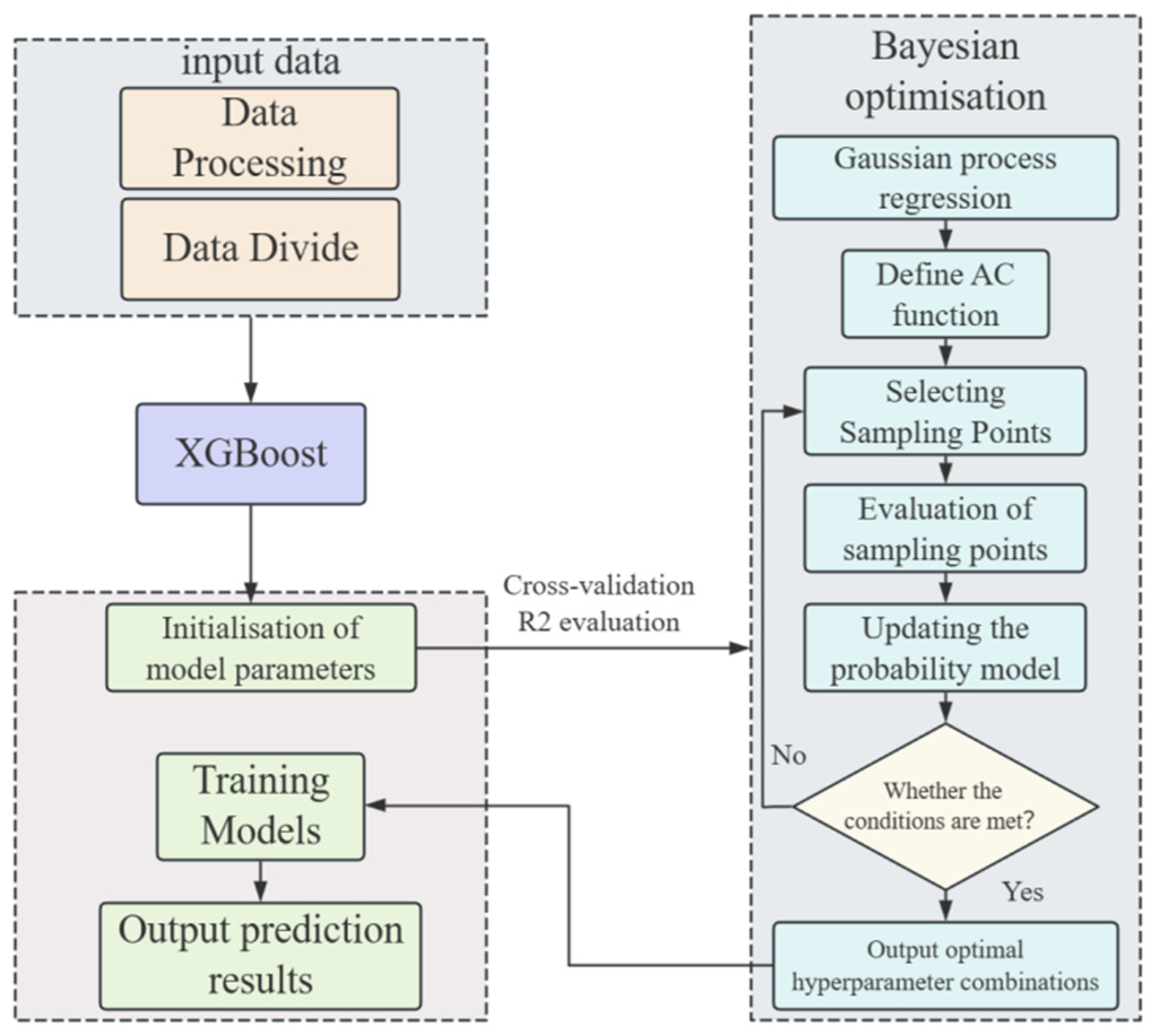
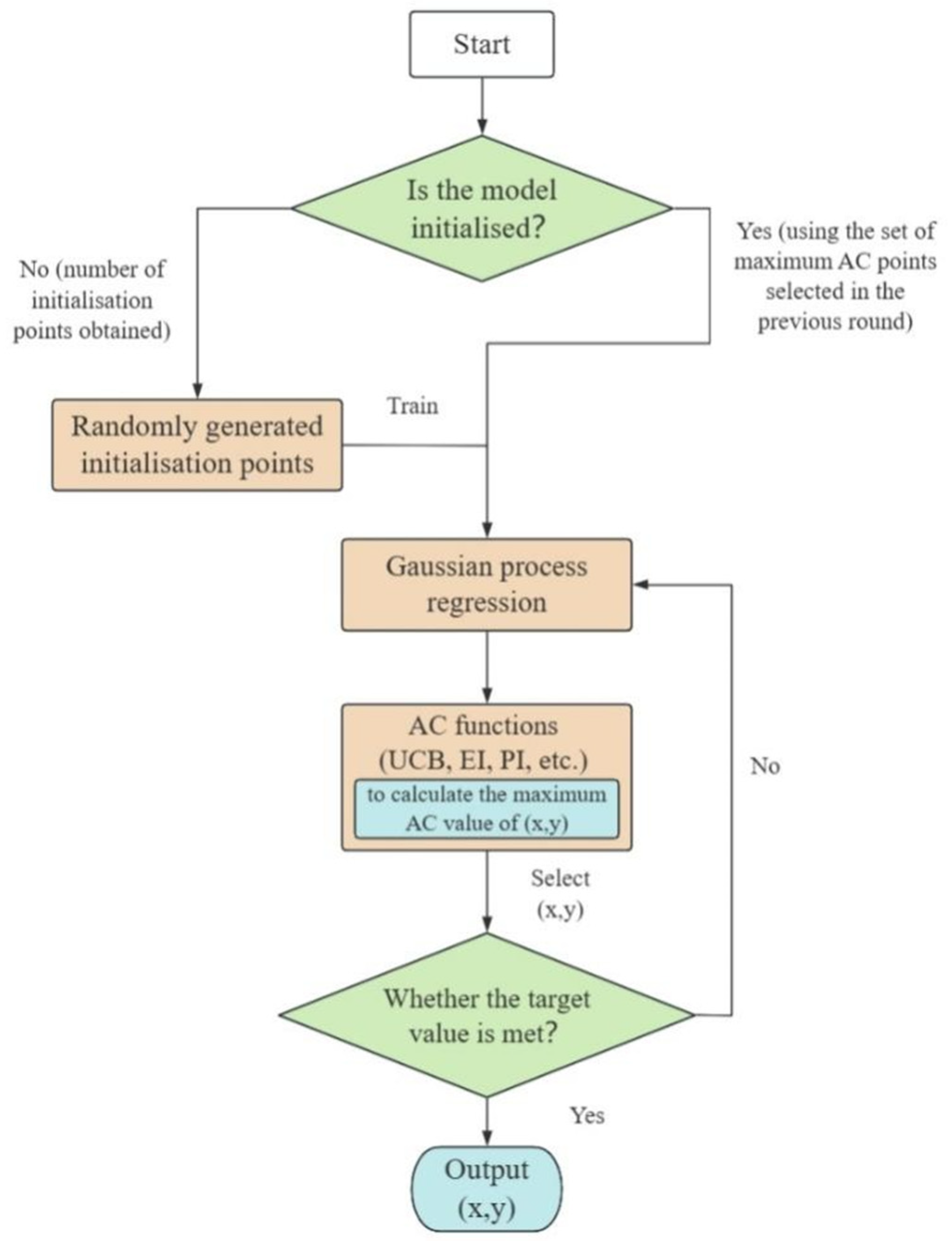
The optimization procedure begins by postulating a prior distribution (commonly a Gaussian model [34]) for the objective function. Through iterative cycles, the algorithm (a) identifies the most promising sampling point based on the current probabilistic model, (b) evaluates the objective function at this point, and (c) updates the probabilistic model with new observations. This cycle repeats until meeting either predefined iteration limits or other termination criteria [35,36]. Figure 1 illustrates this workflow in detail.

Bayesian optimization excels at parameter tuning in machine learning, particularly in scenarios where function cost evaluation is expensive (in terms of time and computation), models are black boxes, and the optimization goal is global optimization. Compared to other optimization methods, Bayesian optimization can leverage past learning results to improve search speed, making informed guesses by combining past knowledge and uncertainty information to search for optimal solutions more efficiently.

4. Engineering Case Study Analysis

4.1. Engineering Background

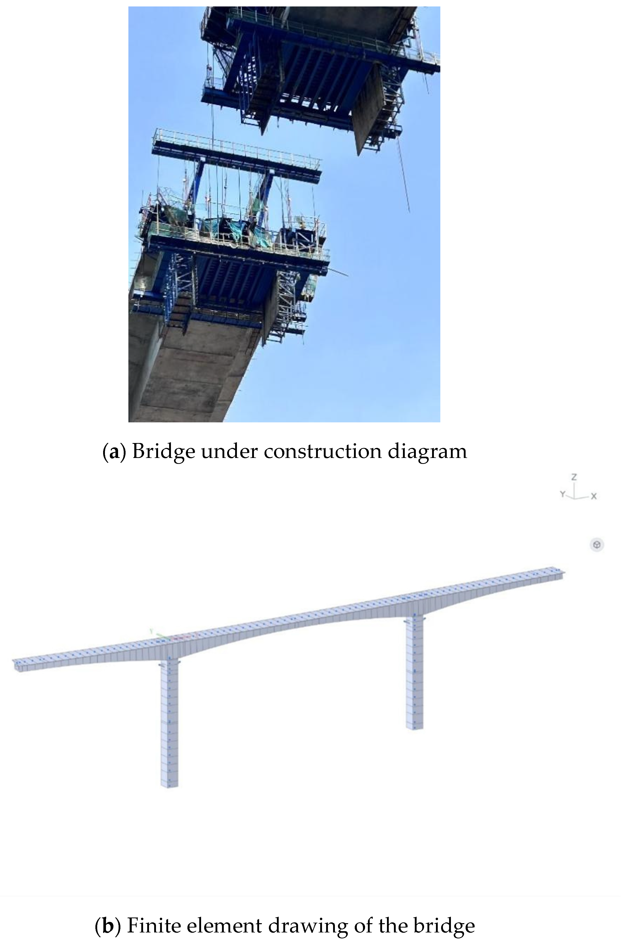
This paper takes a prestressed concrete continuous rigid-frame bridge in Hebi City, Henan Province as its background. The bridge adopts an 85 m + 142 m + 85 m three-span prestressed concrete continuous rigid frame structure, with a split-span layout, a single span width of 12.5 m, and radially arranged piers and abutments. The bottom slab of the box girder is horizontal, and the main girder adopts a single-box, single-cell cross-section. The main piers are single-column hollow piers, with pile caps connected to drilled-shaft pile foundations. The bridge layout diagram is shown in Figure 2.

4.2. Establishment of Finite Element Models

4.2.1. Choosing Finite Element Software

Currently, the main software available for temperature field simulation includes ANSYS, ABAQUS, and Midas Fea. This paper selects the Midas Fea 2022 finite element simulation software to analyze the hydration heat temperature effect on the 0# block (main pier cross-section) of the bridge. Midas Fea is currently the only fully Chinese-localized simulation analysis software specifically designed for the civil engineering field. It features a user-friendly and efficient interface, powerful geometric modeling capabilities, automatic mesh generation functionality, and postprocessing computational analysis capabilities. It can perform various linear and nonlinear analyses, reinforcement simulation, contact analysis, hydration heat analysis, crack analysis, fatigue analysis, and potential flow analysis.

4.2.2. Defining Concrete Material Properties

C55 concrete is used with an elastic modulus of 3.55 × 10⁴ N/mm², a Poisson’s ratio of 0.2, a linear expansion coefficient of 1 × 10⁻⁵, and a mass density of 2.4 × 10³ kg/m³. The value of thermal conductivity is related to the composition of the concrete. When experimental data on the thermal properties of concrete are unavailable, it can be calculated by summing the products of the weight percentages of each component and their respective thermal property coefficients. The thermal conductivity of concrete typically ranges from 8.39 to 12.56 kJ/(m·h·°C). Here, the thermal conductivity of C55 concrete is calculated using an empirical formula is 10.6 kJ/(m·h·°C). The specific heat capacity can be calculated using a weighted average method based on the weight percentages of the concrete components. The typical range for the specific heat capacity of concrete is 0.84 to 1.05 kJ/(kg·°C). The specific heat capacity calculated here is 0.96 kJ/(kg·°C). The specific values for each parameter are summarized in

Table 1. Calculated values of physical parameters of C55 concrete for the main girder of a continuous rigid-frame bridge.

Parameters	Densit γ (g/m3)	Specific Heat c kJ/(kg·°C)	Thermal Conductivit k (kJ/m·h·°C)	Elastic Modulus E (MPa)	Poisson’s Ratio	Hermal Expansion Coefficient
numerical	2400	0.96	10.6	3.55 × 104	0.2	1 × 10−5

:

4.2.3. Define Thermal Parameters

(1) Compressive strength and shrinkage creep of concrete

Time-dependent material properties include concrete shrinkage and creep, and concrete compressive strength. The shrinkage and creep values are taken from the “Design Specifications for Highway Reinforced Concrete and Prestressed Concrete Bridges and Culverts” (JTG 3362-2018). However, there is no specific standard definition method for concrete compressive strength in China. Here, the CEB-FIP standard provided by the software is adopted, and the time-dependent compressive strength curve is shown in Figure 3.

(2) Ambient temperature around the structure

Changes in ambient temperature are one of the key factors affecting the temperature field of hydration heat in box girders. In Midas Fea, there are three modes for defining the ambient temperature around the structure: user-defined, constant, and sine function. Based on the actual temperature changes at the local meteorological station, the following sine function is used to define it:

$$\begin{array}{c}\mathit{T}={\mathit{T}}_0+\mathit{T}\mathit{sin}\left[2{\displaystyle \frac{{\mathit{p}}_{\mathit{i}}}{24}}\left(\mathit{t}+{\mathit{t}}_0\right)\right]\end{array}$$

(9)

Among them, parameter T₀ is the average temperature, parameter T is the temperature change amplitude, and parameter t₀ is the delay time.

(3) Concrete Pouring Temperature

Based on the actual conditions of this project, the concrete pouring temperature is set to 20 °C.

(4) Heat Source Function

The heat source function in Midas FE is defined by specifying the maximum adiabatic temperature rise and thermal conductivity coefficient. The adiabatic temperature rise refers to the temperature increase that would occur if the concrete were in an adiabatic state and unable to dissipate heat externally. Factors influencing this include cement type, cement content, and ambient temperature. Adiabatic temperature rise data is typically obtained through testing; if experimental data is unavailable, the theoretical formula in Reference [37] can be used for estimation.

(5) Convection Coefficient Function

Convective heat transfer refers to the heat exchange phenomenon that occurs when the fluid surrounding an object comes into contact with its surface during flow. For bridge structures, this primarily manifests as air convective heat transfer. The convective heat flux density between the fluid and the solid surface is directly proportional to the temperature difference between the two. During the concrete pouring construction of the bridge’s 0# block, the third-type boundary condition was adopted.

The value of the convection coefficient is influenced by factors such as wind speed, air temperature, and the roughness of the structural surface. Various empirical formulas have been proposed by different scholars based on field experiments to calculate the convective heat transfer coefficient, typically expressed as h_c = a + bv, where the constant a represents the free convection component caused by the temperature difference between the structural surface and the atmosphere; and the product of the constant b and wind speed v represents the forced convection component induced by wind. This study adopts the heat transfer coefficient calculation formula (kJ/m·h·°C) provided by Mirambell [38,39] for different parts of the interior and exterior of concrete box girders:

$$\begin{array}{c}\mathit{T}\mathit{h}\mathit{e} \mathit{u}\mathit{p}\mathit{p}\mathit{e}\mathit{r} \mathit{s}\mathit{u}\mathit{r}\mathit{f}\mathit{a}\mathit{c}\mathit{e} \mathit{o}\mathit{f} \mathit{t}\mathit{h}\mathit{e} \mathit{t}\mathit{o}\mathit{p} \mathit{p}\mathit{l}\mathit{a}\mathit{t}\mathit{e}: {\mathit{h}}_{\mathit{top}}=4.67+3.83{\mathit{v}}_{\mathit{a}}\end{array}$$

(10)

$$\begin{array}{c}\mathit{B}\mathit{o}\mathit{t}\mathit{t}\mathit{o}\mathit{m} \mathit{p}\mathit{l}\mathit{a}\mathit{t}\mathit{e} \mathit{l}\mathit{o}\mathit{w}\mathit{e}\mathit{r} \mathit{s}\mathit{u}\mathit{r}\mathit{f}\mathit{a}\mathit{c}\mathit{e}: {\mathit{h}}_{\mathit{bot}}=2.17+3.83{\mathit{v}}_{\mathit{a}}\end{array}$$

(11)

$$\begin{array}{c}\mathit{T}\mathit{h}\mathit{e} \mathit{o}\mathit{u}\mathit{t}\mathit{e}\mathit{r} \mathit{s}\mathit{u}\mathit{r}\mathit{f}\mathit{a}\mathit{c}\mathit{e} \mathit{o}\mathit{f} \mathit{t}\mathit{h}\mathit{e} \mathit{w}\mathit{e}\mathit{b} \mathit{p}\mathit{l}\mathit{a}\mathit{t}\mathit{e}: {\mathit{h}}_{\mathit{web}}=3.67+3.83{\mathit{v}}_{\mathit{a}}\end{array}$$

(12)

$$\begin{array}{c}{\mathit{Inner} \mathit{surface}: \mathit{h}}_{\mathit{in}}=3.5\end{array}$$

(13)

In the formula, v_a is the average wind speed (m/s).

4.2.4. Monitoring Point Layout and Model Establishment

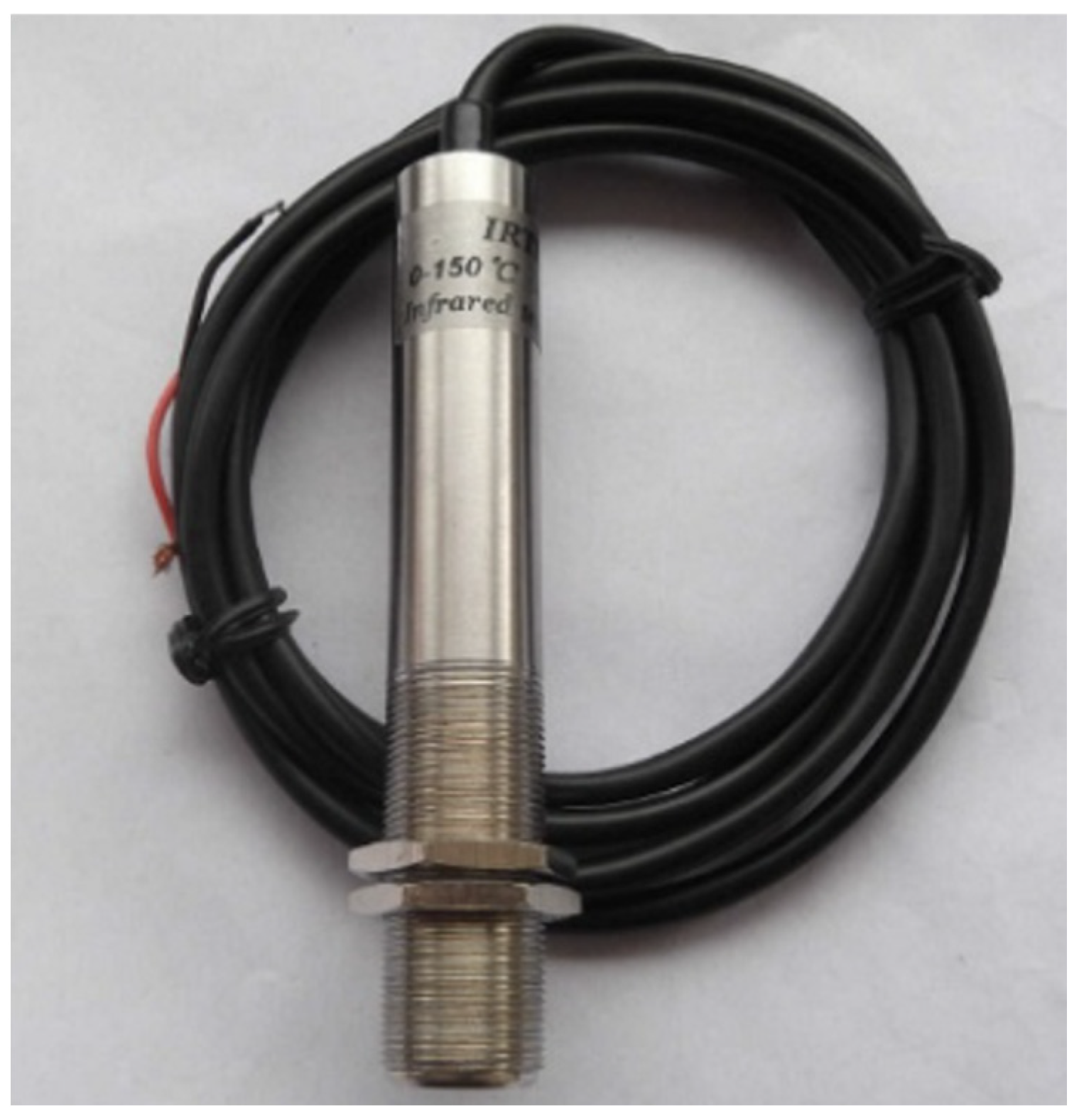
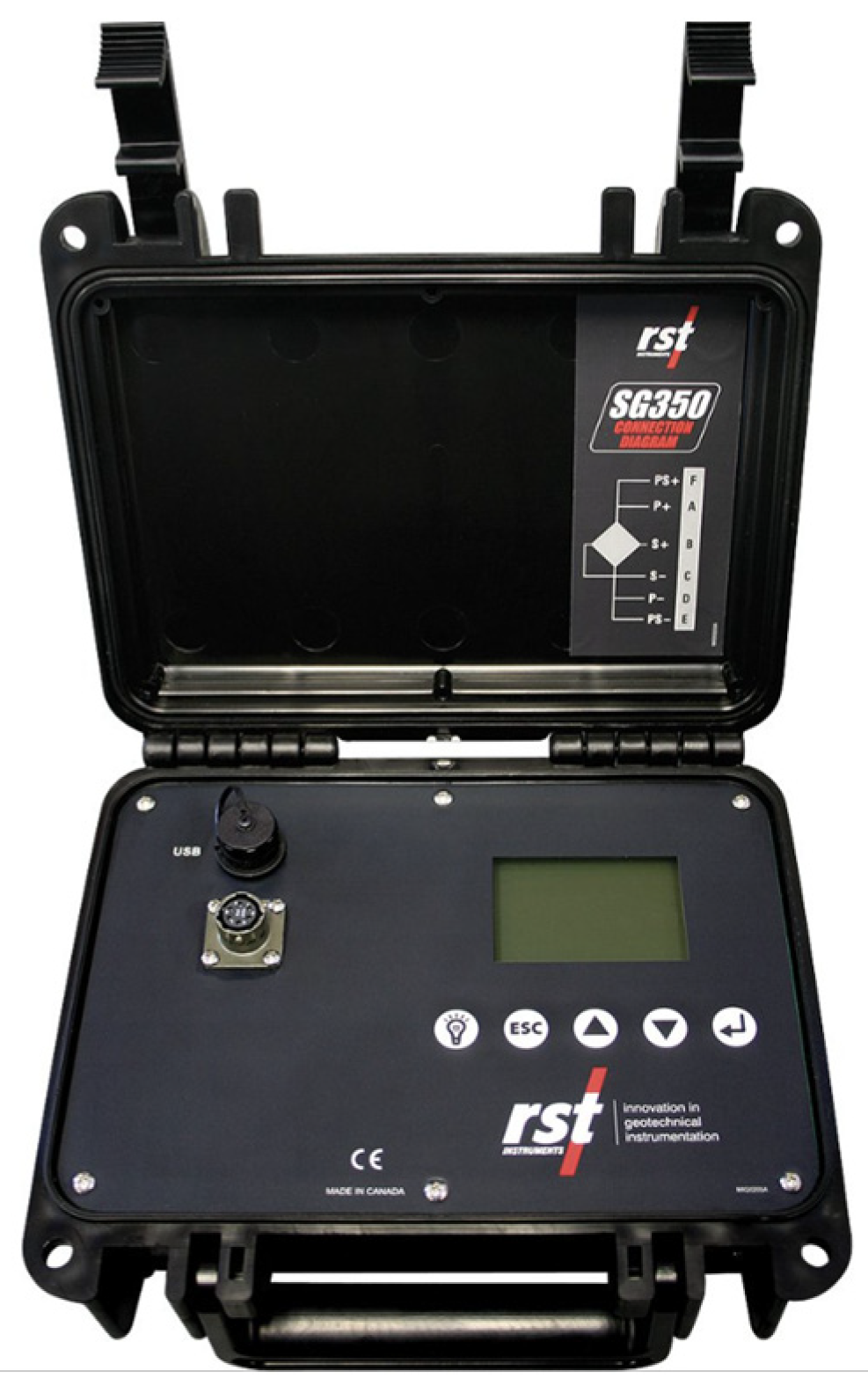
The temperature sensor is a semiconductor-based model manufactured by Chongqing Defei Inspection and Testing Co., Ltd., paired with the company’s proprietary portable data acquisition unit as shown in Figure 4 and Figure 5. This lightweight data logger features a high-capacity built-in lithium battery (4800 mAh/12 V) and is characterized by high precision, low power consumption, and excellent anti-interference capability. With an operational temperature range of −25 °C to 115 °C, the device achieves a measurement accuracy of ±0.6 °C and offers a resolution of 0.2 °C. A single charge supports up to 20 h of continuous operation. The system incorporates data storage functionality with a maximum capacity of 3500 datasets and supports data export via USB interface. The sensor features a stainless steel enclosure, making it suitable for complex environmental monitoring applications. The acquisition unit is equipped with a 1.8-inch LCD screen that provides real-time display and alarm functions for abnormal readings, meeting the requirements for rapid industrial field inspections.

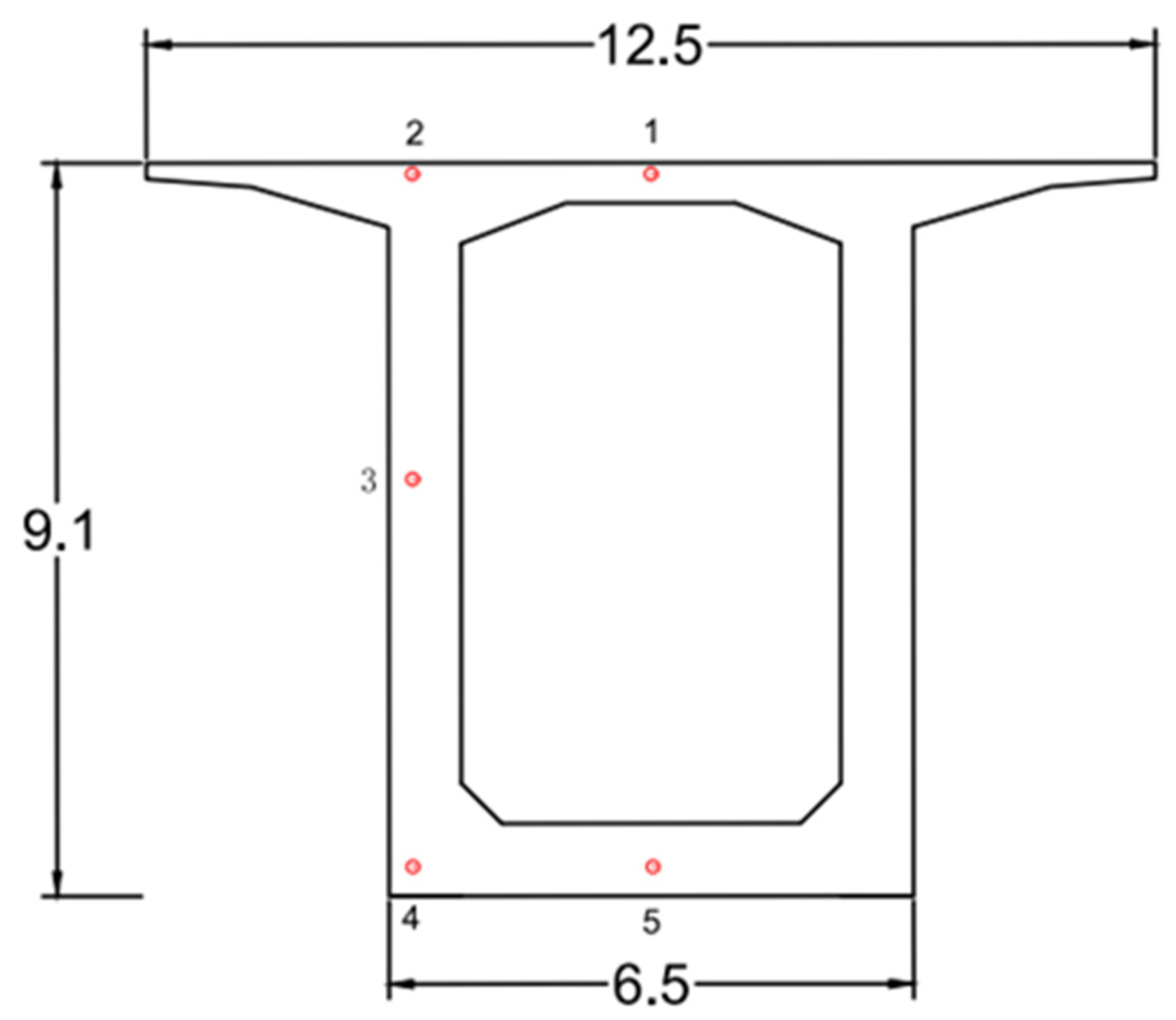
A total of five temperature sensors were installed at the bottom slab, web, and top slab of the box girder. The selection of temperature measurement points on the cross-section took into account the differences in temperature peaks at different locations of the box girder as well as the varying times at which these peaks occur. The locations of the cross-section characteristic points are shown in Figure 6.

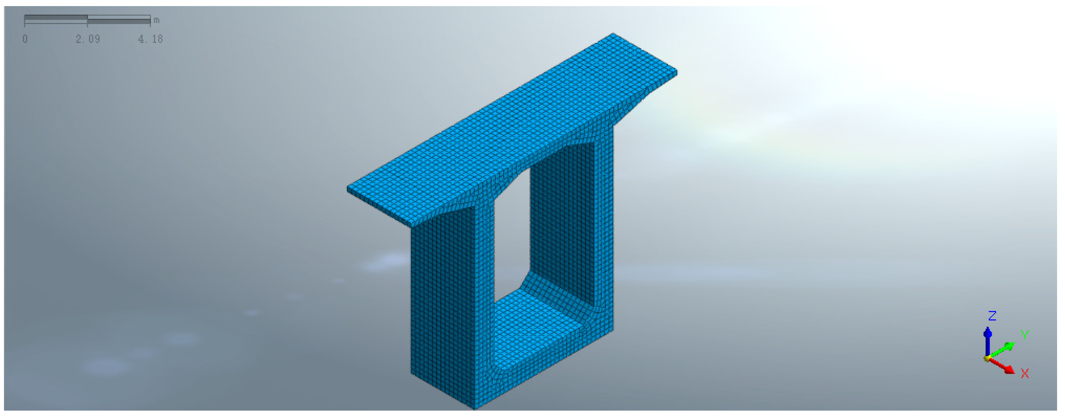
The Midas Fea finite element software was used to establish the geometric solid model of the bridge’s 0# block, and the solid model was meshed (automatic meshing). The element size selected was 0.2 m, and tetrahedral elements were used for meshing. The 0# block was divided into 10,551 elements and 12,961 nodes. The geometric solid model and meshed model are shown in Figure 7. In this solid model, the x-axis represents the longitudinal direction of the bridge, the y-axis represents the transverse direction, and the z-axis represents the vertical direction.

4.3. Range and Level of Counter-Analysis Parameters

The main parameters influencing the temperature field of box girders include specific heat capacity c, density γ, thermal conductivity k, final hydration heat Q₀, pouring temperature T, and convective heat transfer coefficient h. Among these, the specific heat capacity c and density γ of concrete can be directly measured through experiments, generally yielding accurate results with low variability; hence, they are typically not selected as inversion parameters. Given that c and γ are known, the thermal diffusivity d can be derived from the mathematical relationship with thermal conductivity k once either parameter is determined. Therefore, this study selects thermal conductivity k for inversion to represent the thermal diffusion characteristics. The pouring temperature T is a construction-controlled variable that can be directly obtained through on-site measurement during casting, offering high certainty and thus is excluded from the inversion parameters. In contrast, the convective heat transfer coefficient h is significantly influenced by actual environmental conditions (such as wind speed, surface roughness, and airflow patterns), making it difficult to accurately calculate using theoretical formulas. Its value may vary both temporally and spatially, necessitating its inclusion as a parameter to more realistically represent the heat exchange behavior at structural boundaries. Furthermore, the hydration reaction process critically affects the development of the temperature field. This study employs a double exponential function to describe the hydration heat release process, wherein the reaction rate coefficient m governs the pattern of heat release. This parameter is associated with cement type, admixtures, and environmental conditions, and is difficult to measure directly; thus, it also requires estimation through inversion. In summary, the following five parameters are ultimately selected for inversion: thermal conductivity k, final hydration heat Q₀, convective heat transfer coefficient at the top surface of the roof h_top, convective heat transfer coefficient at the outer surface of the web h_web, and reaction rate coefficient m. This selection takes into account both the measurability and sensitivity of the parameters, while also ensuring the rationality of the model and its practical applicability in engineering. The value ranges for each parameter are provided in

Table 2. Range of values for each parameter.

Factor	k (kJ/m·h·°C)	Q0 (KJ/kg)	Htop (KJ/m2·h·°C)	Hweb (KJ/m2·h·°C)	m
range	8.50~12.50	150~550	16.80~99.54	13.20~95.94	0.30~0.40

.

4.4. Sample Data Orthogonal Experiment

Through numerical simulation-based single-parameter sensitivity analysis of bridge design parameters, the individual influence of each parameter on mechanical performance can be revealed. However, this approach has significant limitations: by keeping other parameters fixed, it fails to capture interaction effects between parameters, which restricts the representativeness and applicability of the resulting dataset. If a full factorial experimental design is used to investigate multiparameter effects, the number of parameter combinations increases exponentially, leading to large-scale experiments with high costs and long durations. To address this issue, orthogonal experimental design can be introduced [40]. This method uses orthogonal arrays to select representative experimental points with uniformity and comparability, enabling effective investigation of multiparameter and interaction effects with a significantly reduced number of tests, while ensuring result reliability and improving experimental efficiency. The specific procedures include determining parameters and levels, selecting an orthogonal array, developing an experimental plan, and conducting the tests. In this study, an orthogonal experimental design was employed to construct the numerical simulation scheme and generate a dataset of thermal parameters [41,42].

Analysis determined the number of levels for six parameters (two 9-level, two 7-level, and one 6-level parameters). An L_a(9^c) orthogonal table was selected, with the quasi-level method used to accommodate multi-level parameters. The experimental plan is detailed in

Table 3. Levels of influence factors in the experiment.

Levels	Parameters
	k	Q0	htop	hweb	m
1	8.5	150	16.80	13.20	0.30
2	9.0	200	30.60	27.00	0.32
3	9.5	250	44.39	40.79	0.34
4	10.0	300	58.18	54.58	0.36
5	10.5	350	71.96	68.36	0.38
6	11.0	400	85.80	82.15	0.40
7	11.5	450	99.54	95.94
8	12.0	500
9	12.5	550

.

4.5. Predictive Modeling

Based on the XGBoost model, five inversion prediction models were established for thermal conductivity k, final hydration heat Q₀, convection coefficient h_top on the top surface of the slab, convection coefficient h_web on the outer surface of the web, and reaction coefficient m.

4.5.1. Data Preprocessing

In this study, the results of numerical simulation experiments were used as the dataset, and data preprocessing was required before model construction. The selected input feature variables were the temperature peaks at five monitoring points. The output feature variables were thermal conductivity k, final hydration heat Q₀, convection coefficient on the top surface h_top, convection coefficient on the outer surface of the web h_web, and reaction coefficient m. The model was constructed by dividing the dataset into a training set and a test set. The training set was used to train the model, and the test set was used to evaluate the performance of the constructed model. The training samples were obtained through finite element calculations, totaling 81 sets, which were divided into a training set and a test set in an 8:2 ratio. The training set served as the training data for the inversion model, while the test set was used to assess the inversion performance of the model.

4.5.2. Model Evaluation Metrics

To ensure reliability, five-fold cross-validation is employed. The implementation process is as follows: First, the original dataset is divided into five subsets of similar distribution, without overlapping, using stratified sampling. Next, five iterative training rounds are conducted, with four subsets serving as training data and the remaining one as the validation set in each round. The final model’s performance metrics are derived from the average of the five validation results [43]. This approach, combining Bayesian optimization with cross-validation, not only enhances parameter search efficiency but also improves the model’s generalization ability, thereby mitigating overfitting.

This study falls under the category of regression problems, with common evaluation metrics including root mean square error (RMSE), mean absolute error (MAE), and coefficient of determination (R²). RMSE and MAE reflect the deviation between predicted values and actual values, with smaller values indicating higher accuracy; R² measures the model’s ability to explain data variability, with values closer to 1 indicating stronger linear correlation between predicted and actual values.

5. Results and Discussion

5.1. Hyperparameter Optimization Results

In this paper, the number of iterations for the Bayesian optimization algorithm is set to 50, ensuring both rapid convergence and accuracy. During the optimization process, the average R² from five-fold cross-validation is used as the core evaluation metric to select the optimal hyperparameter combination, ensuring the stability and reliability of the model performance. As shown in Figure 8, the BO-XGBoost flowchart clearly illustrates the complete optimization process from parameter initialization, proxy model construction, to optimal parameter selection.

Table 4. Hyperparameter ranges and optimization results.

Model	Hyperparameters	Range	k	Q0	htop	hweb	m
	n_estimators	(10, 500)	287	357	165	355	314
	min_child_weight	(1, 11)	5	8	3	1	6
XGBoost	max_depth	(1, 11)	7	4	2	2	5
	learning_rate	(0.01, 0.3)	0.04	0.029	0.221	0.205	0.08
	subsample	(0.7, 1)	1	0.897	0.7	1	1

presents the hyperparameter ranges and final optimization results of the Bayesian optimization.

5.2. Model Prediction Results

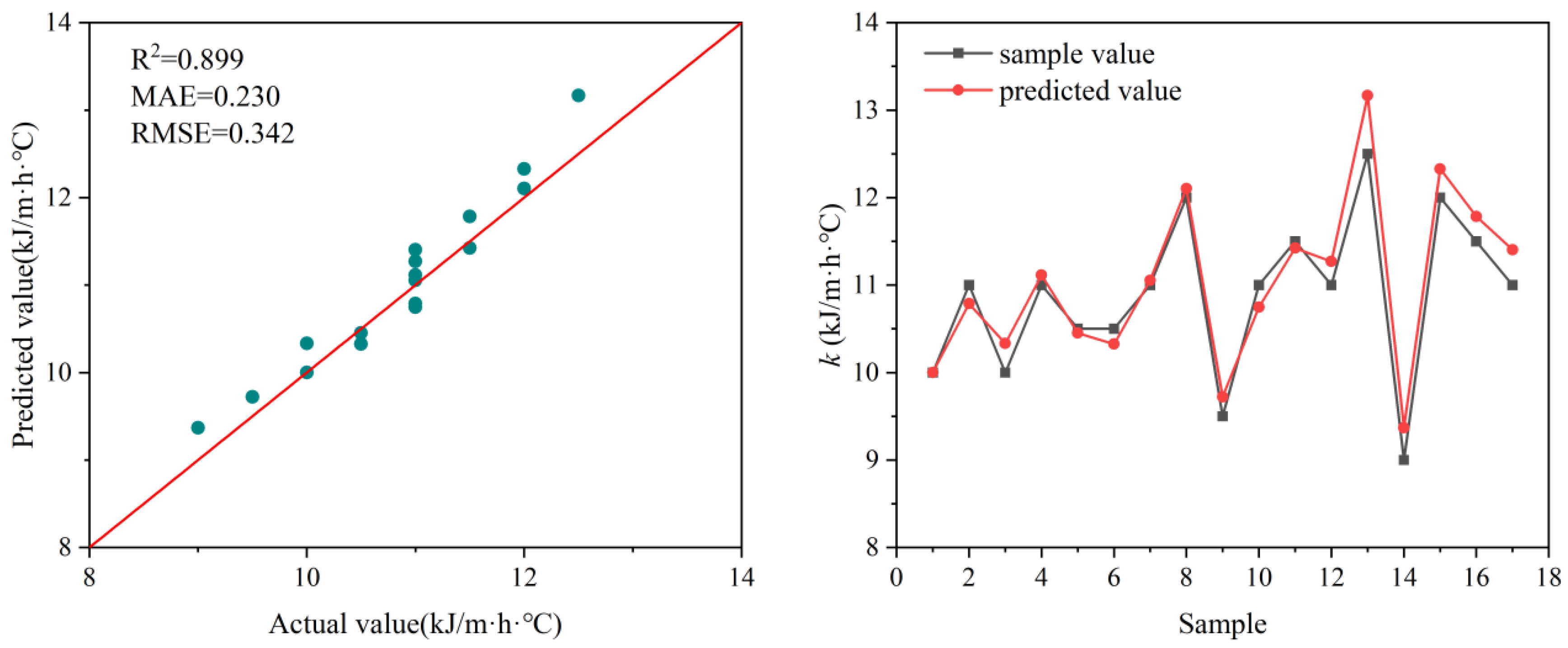
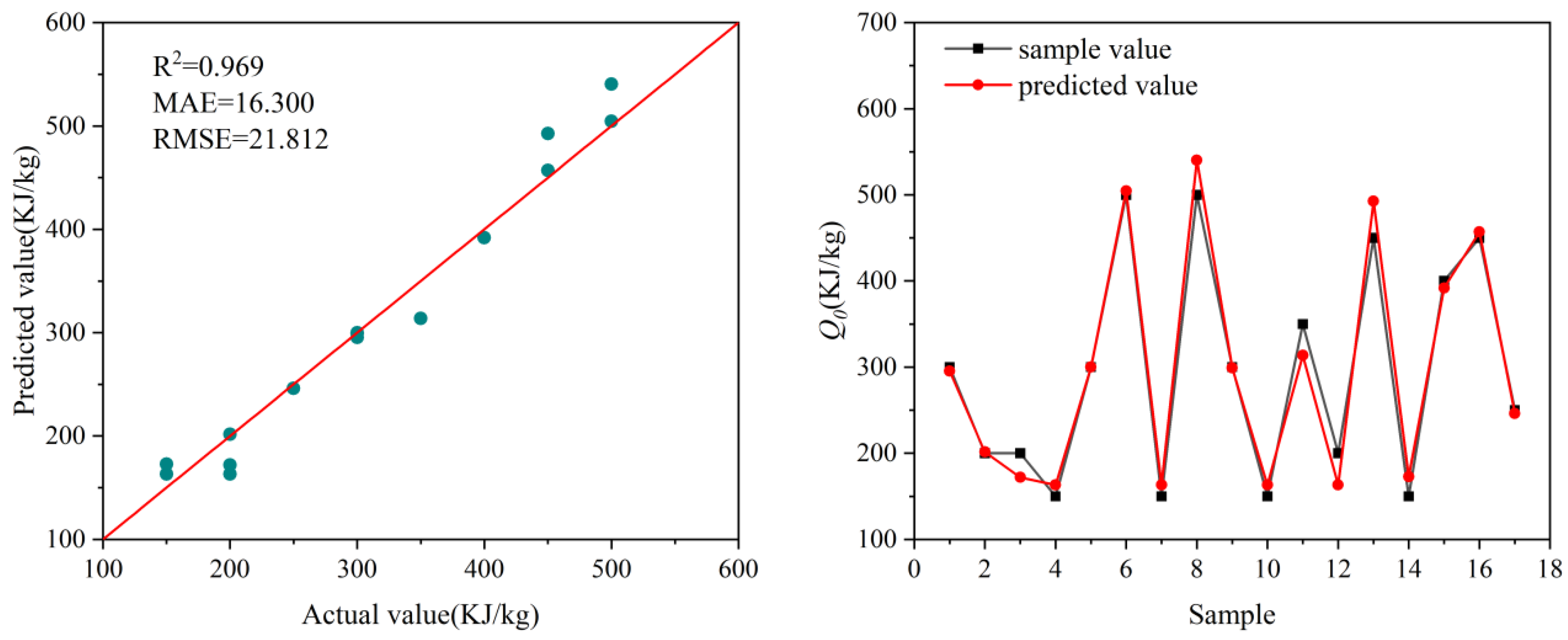
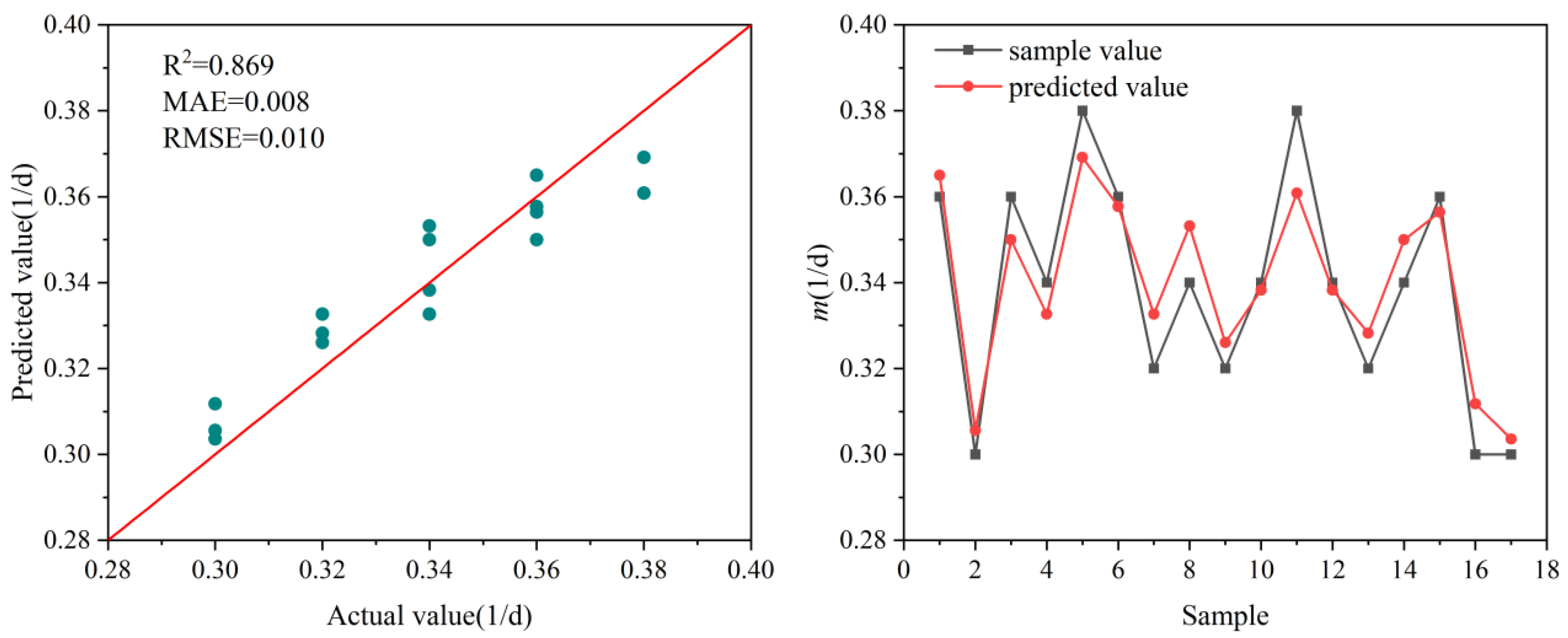
After training the model and completing hyperparameter optimization, the model’s predictive performance was validated using the test set. The test set contained 16 sets of sample data, covering five thermal parameter prediction models. By comparing the predicted values with the actual values, the model’s accuracy and generalization ability were analyzed, as shown in Figure 9, Figure 10, Figure 11, Figure 12 and Figure 13. The figures show the relationship between the predicted values and actual values for each of the five parameter models in the test set, as well as the relative error between the predicted values and actual values in the test set. It can be seen that the hydration heat coefficient model has the highest accuracy and the smallest fluctuation in relative error, followed by the convection coefficient h_top on the upper surface of the top plate and the convection coefficient h_web on the outer surface of the web plate; however, the accuracy of the thermal conductivity coefficient k and the reaction coefficient m is relatively lower, though they still meet engineering requirements. Additionally, the test set data points are almost all near the 1:1 error line, which fully demonstrates its excellent generalization capability. The table shows the evaluation metrics for each parameter model.

5.3. Compared with Traditional Machine Learning Models

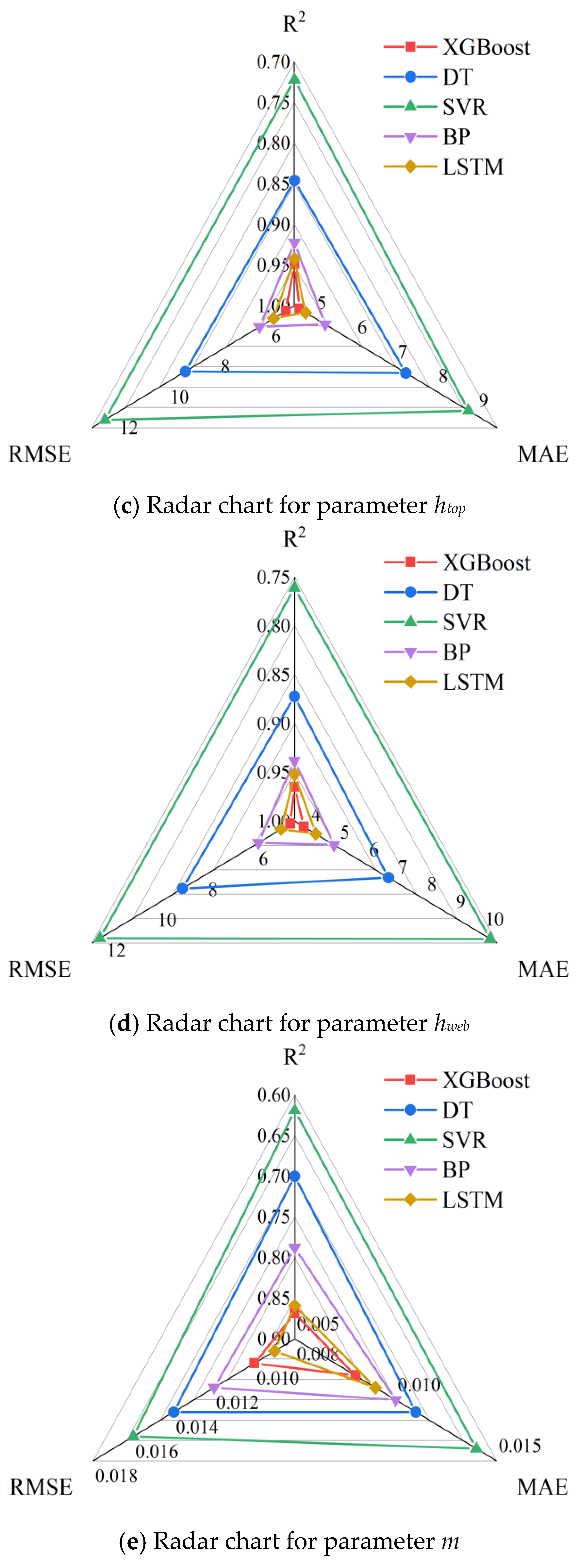
According to the data presented in

Table 5. Comparison with traditional machine learning models.

Model	Evaluation Metrics	Parameters
		k	Q0	htop	hweb	m
XGBoost	R2	0.899	0.969	0.949	0.965	0.869
	MAE	0.230	16.300	4.626	3.828	0.008
	RMSE	0.342	21.812	5.338	4.670	0.010
DT	R2	0.768	0.952	0.846	0.872	0.7
	MAE	0.351	22.710	7.253	6.742	0.011
	RMSE	0.426	27.076	9.307	8.923	0.014
SVR	R2	0.709	0.958	0.722	0.761	0.619
	MAE	0.400	18.897	8.795	10.257	0.014
	RMSE	0.476	25.190	12.486	12.183	0.016
BP	R2	0.815	0.960	0.922	0.938	0.788
	MAE	0.298	18.214	5.259	4.866	0.010
	RMSE	0.388	24.048	6.378	5.924	0.012
LSTM	R2	0.845	0.966	0.942	0.952	0.859
	MAE	0.267	17.122	4.775	4.231	0.009
	RMSE	0.359	22.768	5.822	5.028	0.009

, significant differences can be observed in the performance of various machine learning models for thermal parameter inversion, as further illustrated in the radar chart in Figure 14. Specifically, compared to the DT model, the XGBoost model achieved an improvement in R² ranging from 1.8% to 24%, while reducing MAE by 27.3% to 43.2% and RMSE by 28.6% to 47.7%. Relative to the SVR model, XGBoost showed an increase in R² between 1.1% and 40.4%, along with a reduction in MAE of 42.8% to 62.7% and in RMSE of 37.5% to 61.7%. When compared to the BP model, XGBoost improved R² by 0.3% to 10.3%, decreased MAE by 3.0% to 22.8%, and lowered RMSE by 1.9% to 11.9%. In contrast to the LSTM model, XGBoost attained a gain in R² of 0.3% to 6.4%, a reduction in MAE of 1.2% to 13.9%, and a decrease in RMSE of 0.5% to 5.0%. Although the performance of the LSTM model is competitive with that of XGBoost, its training time is substantially longer. These results fully demonstrate the superior predictive capability and efficiency of the XGBoost model.

5.4. Inverse Modeling of Observed Data

In order to verify the applicability and accuracy of the BO-XGBoost model in actual engineering applications, this study took the construction of pier 0# of a prestressed concrete continuous rigid-frame bridge as an example and performed an inverse analysis of the thermal parameters of the concrete box girder. Through on-site temperature monitoring experiments, measured temperature peak data from five characteristic points were obtained and input into the pre-trained BO-XGBoost model, yielding the inversion values of the thermal parameters. The inversion results are shown in

Table 6. Comparison of parameter inversion values and calculated values.

	Parameters
	k	Q0	htop	hweb	m
calculated value	10.6	350.00	58.18	54.58	0.362
inversion value	10.9	343.69	75.64	24.26	0.377

.

As shown in Table 6, except for the convection coefficient h, the differences between the inversion values of the remaining three parameters and the calculated values obtained using empirical formulas are relatively small. The relative error for the thermal conductivity coefficient k is 2.8%, the relative error for the final hydration heat Q₀ is 1.8%, and the relative error for the reaction coefficient m is 4.1%. However, the error between the inversion value of the convection coefficient and the calculated value based on the empirical formula is relatively large. This is primarily because the empirical formula relies on local average wind speed data and cannot reflect the changes in wind speed in real time at different locations of the box girder. In contrast, inversion analysis can more accurately capture the influence of actual wind speed distribution, thereby obtaining convection coefficient values that better align with actual engineering conditions. This result validates the effectiveness of the inversion method in addressing complex boundary condition problems.

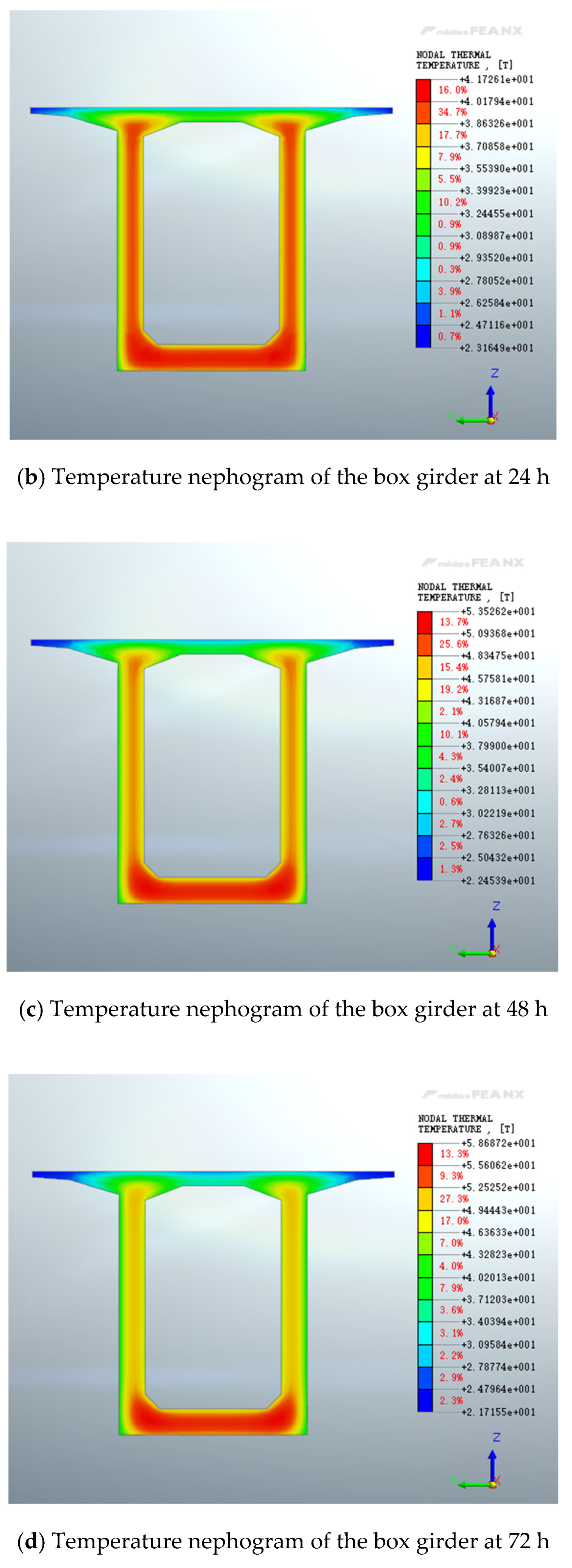
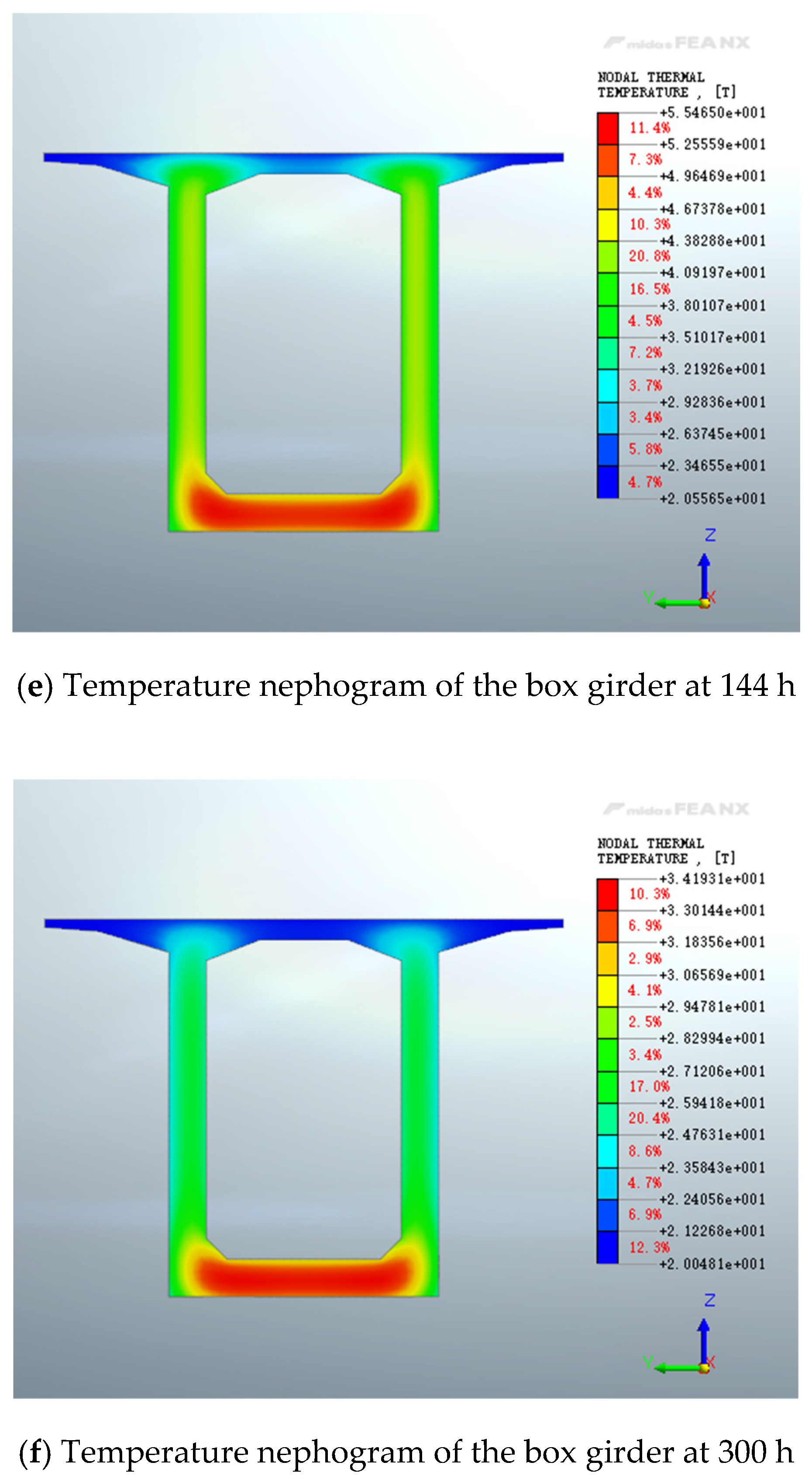
To further validate the reliability of the inversion results, the thermal parameter values obtained from empirical formulas and those derived from inversion were separately input into a finite element model for comparative analysis. Due to space limitations, only the temperature nephograms of the box girder calculated using the inversion parameters are presented, as shown in Figure 15. These correspond to six typical time points: 12 h, 24 h, 48 h, 72 h, 144 h, and 300 h after pouring. It can be observed from the figure that as the hydration reaction proceeds, the internal temperature of the box girder gradually increases, reaches a peak at a certain point, and then gradually decreases until it stabilizes the ambient temperature. The temperature distribution exhibits a clear gradient pattern, with higher temperatures in the central region decreasing toward the surfaces, which aligns with the typical behavior of mass concrete under hydration heat effects.

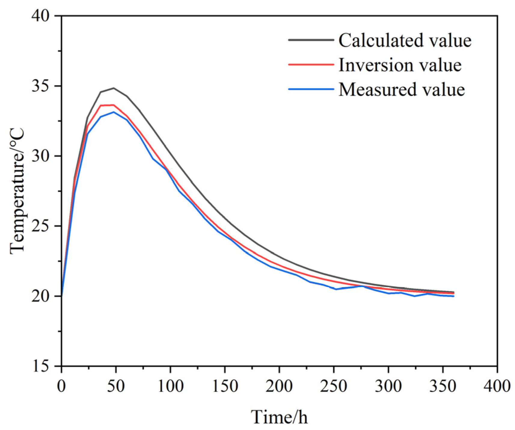
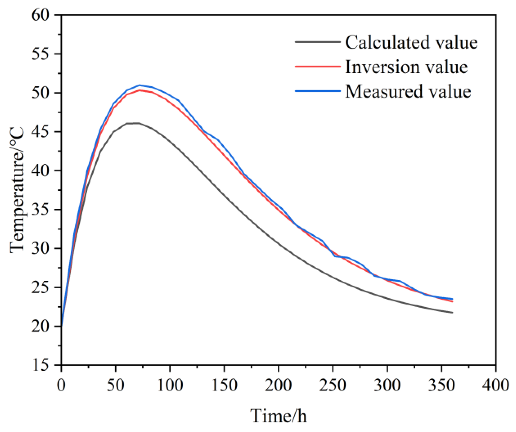
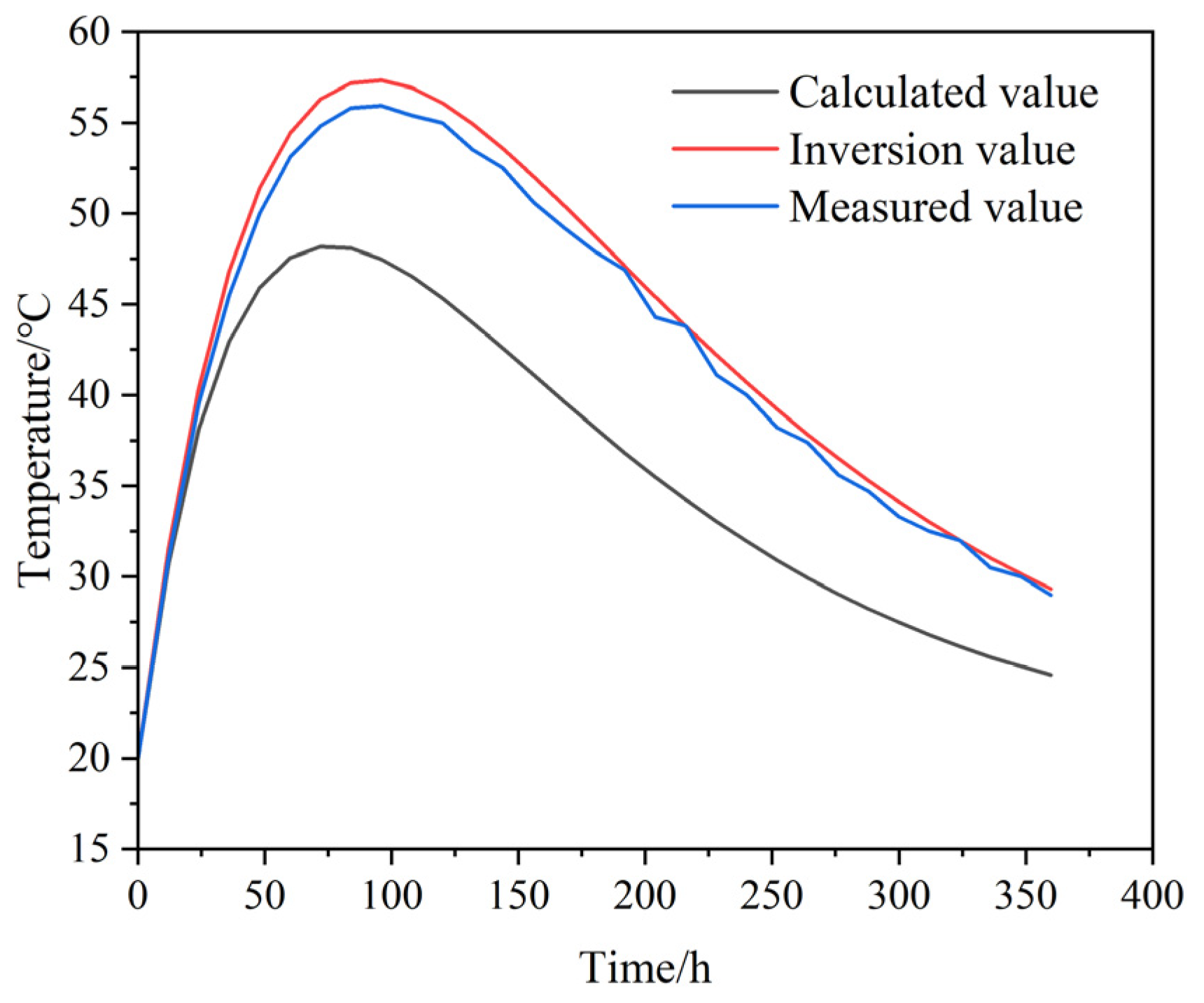
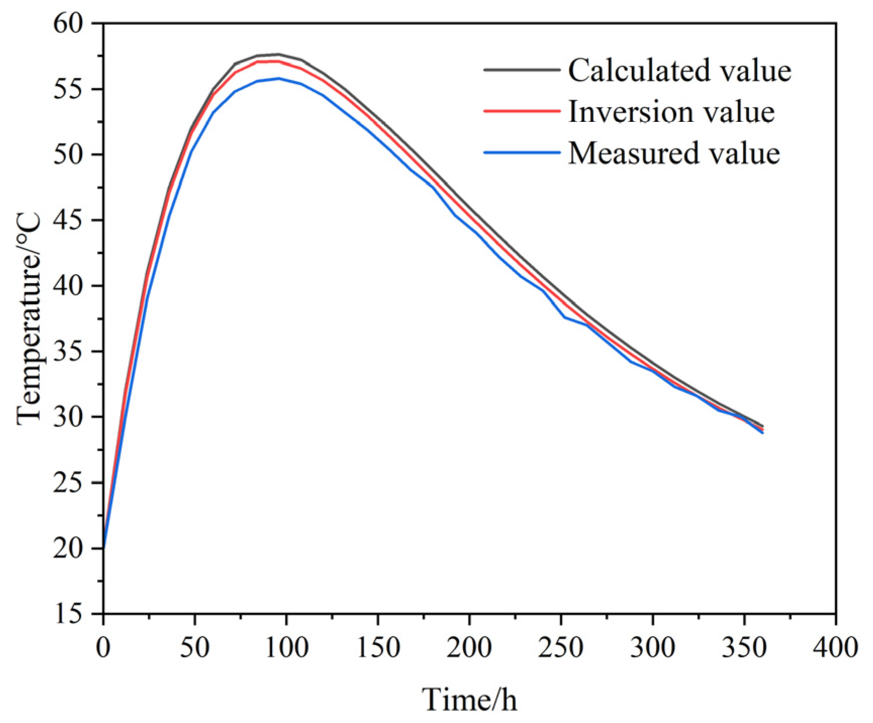
The recalculated temperature variation curves and peak temperatures at the five characteristic points were compared with the actual measured values during the construction process, as shown in Figure 16, Figure 17, Figure 18, Figure 19 and Figure 20 and

Table 7. Comparison of peak temperature results for characteristic points.

	Feature Point Temperature Peak/°C
	1	2	3	4	5
measured value	33.14	38.8	51.61	55.92	55.80
calculated value	34.85	39.69	46.05	48.17	57.62
inversion value	33.62	39.08	50.34	57.32	57.09

. It can be observed that the calculated values based on empirical formulas deviate significantly from the measured values, whereas the inversion values exhibit smaller errors and follow trends similar to the measured data. Specifically, for characteristic point 1, the measured value was 33.14 °C and the inversion value was 33.62 °C, resulting in an error of 0.48 °C. For characteristic point 2, the measured value was 38.8 °C and the inversion value was 39.08 °C, with an error of 0.28 °C. At characteristic point 3, the measured value was 51.61 °C and the inversion value was 50.34 °C, yielding an error of 1.27 °C. For characteristic point 4, the measured value was 55.92 °C and the inversion value was 57.32 °C, resulting in an error of 1.40 °C. At characteristic point 5, the measured value was 55.80 °C and the inversion value was 57.09 °C, with an error of 1.29 °C. The maximum error occurred at characteristic point 4, which was 1.40 °C, corresponding to a relative error of 2.5%. These results indicate that the thermal parameters’ inversion by the BO-XGBoost model align well with the actual construction conditions of the concrete. The inversion values are accurate and reliable, effectively reflecting the internal temperature distribution patterns of the box girder.

6. Conclusions

To address the issue of temperature-induced cracks commonly observed during the construction of concrete box girders, this paper proposed an inverse analysis method integrating orthogonal experimental design with the BO-XGBoost algorithm. The method establishes a nonlinear mapping between temperature peaks at key monitoring points and thermal parameters, enabling accurate inversion of critical thermal properties. Based on the numerical simulations and experimental validation, the following conclusions can be drawn:

(1) The combination of orthogonal experimental design and finite element modeling effectively generated a representative dataset of 81 samples. The BO-XGBoost model successfully captured the complex nonlinear relationships between temperature peaks and thermal parameters, providing a reliable and efficient approach for parameter inversion.

(2) The BO-XGBoost model demonstrated superior performance compared to traditional machine learning models (DT, SVR, BP, and LSTM). It achieved improvements in R² ranging from 0.3% to 40.4%, and reductions in MAE and RMSE by up to 62.7% and 61.7%, respectively. These results confirm the model’s high accuracy, robustness, and efficiency in handling complex nonlinear regression tasks.

(3) Validation through finite element simulations showed that the inversion parameters yielded temperature curves and peak values that were highly consistent with field measurements. The maximum absolute error was 1.40 °C (relative error 2.5%), demonstrating the practical accuracy and engineering applicability of the proposed method. This approach provides a reliable basis for temperature control during construction, effectively mitigating thermal cracking risks.

(4) Although validated on a prestressed concrete continuous rigid-frame bridge, the proposed method exhibits strong generalizability and can be extended to other mass concrete structures such as dams, foundations, and large-scale infrastructure projects, offering broad potential for temperature field analysis and crack prevention.

Despite its promising results, this study has certain limitations. The inversion accuracy for convective heat transfer coefficients remains influenced by empirical wind speed assumptions, which may not fully capture real-time spatial variations. Future research could incorporate real-time environmental monitoring data (e.g., distributed wind speed and solar radiation sensors) to further refine boundary conditions. Additionally, the method could be extended to include time-varying thermal parameters and probabilistic inversion frameworks to enhance robustness under uncertain conditions. Further applications to more complex structural forms and environmental scenarios are also recommended.

References

1. Chen, D.; Guo, W.; Wu, B.; Shi, J. Service life prediction and time-variant reliability of reinforced concrete structures in harsh marine environment considering multiple factors: A case study for Qingdao Bay Bridge. Eng. Fail. Anal. 2023, 154, 107671. [Google Scholar] [CrossRef]
2. Liu, Y.; Pang, B.; Wang, Y.; Shi, C.; Zhang, B.; Guo, X.; Zhou, S.; Wang, J. Life-cycle maintenance strategy of bridges considering reliability, environment, cost and failure probability CO2 emission reduction: A bridge study with climate scenarios. J. Clean. Prod. 2022, 379, 134740. [Google Scholar] [CrossRef]
3. Zhu, Y.; Sun, D.; Guo, H.; Shuang, M. Fine analysis for non-uniform temperature field and effect of railway truss suspension bridge under solar radiation. J. Constr. Steel Res. 2023, 210, 108098. [Google Scholar] [CrossRef]
4. Li, L.; Shan, Y.; Jing, Q.; Yan, Y.; Xia, Z.; Xia, Y. Global temperature behavior monitoring and analysis of a three-tower cable-stayed bridge. Eng. Struct. 2023, 295, 116855. [Google Scholar] [CrossRef]
5. Fan, J.-S.; Li, B.-L.; Liu, C.; Liu, Y.-F. An Efficient Model for Simulation of Temperature Field of Steel-Concrete Composite Beam Bridges; Proceedings of the Structures; Elsevier: Amsterdam, The Netherlands, 2022. [Google Scholar]
6. He, J.; Wang, Z.; Vasdravellis, G.; Wang, L.; Xin, H.; Correia, J.; Berto, F. Fatigue tests and fatigue-life prediction models for hybrid welded-bolted demountable shear connectors. Int. J. Fatigue 2023, 175, 107826. [Google Scholar] [CrossRef]
7. Wei, D.; Du, C.; Lin, Y.; Chang, B. Impact factors of hydration heat of cemented tailings backfill based on multi-index optimization. Case Stud. Therm. Eng. 2020, 18, 100601. [Google Scholar] [CrossRef]
8. Cai, Y.; Wang, F.; Zhao, Z.; Lyu, Z.; Wang, Y.; Zou, P. Early-Hydration Heat and Influencing Factor Analysis of Large-Volume Concrete Box Girder Based on Equivalent Age; Proceedings of the Structures; Elsevier: Amsterdam, The Netherlands, 2023. [Google Scholar]
9. Han, S.; Liu, Y.; Lyu, Y.; Liu, J.; Zhang, N. Numerical simulation investigation on hydration heat temperature and early cracking risk of concrete box girder in cold regions. J. Traffic Transp. Eng. 2023, 10, 697–720. [Google Scholar] [CrossRef]
10. Wang, T.; Cai, J.; Feng, Q.; Jia, W.; He, Y. Experimental Study and Numerical Analysis of Hydration Heat Effect on Precast Prestressed Concrete Box Girder. Buildings 2025, 15, 859. [Google Scholar] [CrossRef]
11. Zhang, P.; Xiong, H.; Wang, R. Measurements and numerical simulations for cast temperature field and early-age thermal stress in zero blocks of high-strength concrete box girders. Adv. Mech. Eng. 2022, 14, 16878132221091514. [Google Scholar] [CrossRef]
12. Kim, M.O.; Bordelon, A.C.; Lee, N.K. Early-age crack widths of thin fiber reinforced concrete overlays subjected to temperature gradients. Constr. Build. Mater. 2017, 148, 492–503. [Google Scholar] [CrossRef]
13. Olajide, O.; Nokken, M.; Sanchez, L. Evaluation of the induced mechanical deterioration of ASR-affected concrete under varied moisture and temperature conditions. Cem. Concr. Compos. 2025, 157, 105942. [Google Scholar] [CrossRef]
14. Du, T.; Cai, Y.; Guo, Y.; Chen, J.; Chen, S.; Yuan, M.; Qu, F. Time-dependent model for in-situ concrete carbonation depth under combined effects of temperature and relative humidity. Case Stud. Constr. Mater. 2025, 22, e04379. [Google Scholar] [CrossRef]
15. Zhang, N.; Mao, T.; Chen, H.; Lv, L.; Wang, Y.; Yan, Y. Temperature prediction for expressway pavement icing in winter based on XGBoost–LSTNet variable weight combination model. J. Transp. Eng. Part A Syst. 2023, 149, 04023062. [Google Scholar] [CrossRef]
16. Kebede, Y.B.; Yang, M.-D.; Huang, C.-W. Real-time pavement temperature prediction through ensemble machine learning. Eng. Appl. Artif. Intell. 2024, 135, 108870. [Google Scholar] [CrossRef]
17. Fard, F.; Sadeghi, N.F.F. Development and utilization of bridge data of the United States for predicting deck condition rating using random forest, XGBoost, and artificial neural network. Remote Sens. 2024, 16, 367. [Google Scholar] [CrossRef]
18. Chen, M.; Xin, J.; Tang, Q.; Hu, T.; Zhou, Y.; Zhou, J. Explainable machine learning model for load-deformation correlation in long-span suspension bridges using XGBoost-SHAP. Dev. Built Environ. 2024, 20, 100569. [Google Scholar] [CrossRef]
19. Guo, Y.; Wang, H.; Guo, Y.; Zhong, M.; Li, Q.; Gao, C. System operational reliability evaluation based on dynamic Bayesian network and XGBoost. Reliab. Eng. Syst. Saf. 2022, 225, 108622. [Google Scholar] [CrossRef]
20. Chen, M.; Park, Y.; Mangalathu, S.; Jeon, J.S. Effect of data drift on the performance of machine-learning models: Seismic damage prediction for aging bridges. Earthq. Eng. Struct. Dyn. 2024, 53, 4541–4561. [Google Scholar] [CrossRef]
21. He, J.; Xin, H.; Wang, Y.; Correia, J.A. Effect of Temperature Loading on the Performance of a Prestressed Concrete Bridge in Oklahoma: Probabilistic Modelling; Proceedings of the Structures; Elsevier: Amsterdam, The Netherlands, 2021. [Google Scholar]
22. Qiao, Y.; Xiong, X. Simultaneous determination of the space-dependent source and initial value for a two-dimensional heat conduction equation. Comput. Math. Appl. 2023, 147, 25–37. [Google Scholar] [CrossRef]
23. Balan, R.; Kaliveeran, V. Thermal buckling of steel tube using finite element method. In Materials Today: Proceedings; Elsevier: Amsterdam, The Netherlands, 2023. [Google Scholar]
24. Zhou, L.; Lv, J.; Cui, M.; Peng, H.; Gao, X. A polygonal element differential method for solving two-dimensional transient nonlinear heat conduction problems. Eng. Anal. Bound. Elem. 2023, 146, 448–459. [Google Scholar] [CrossRef]
25. Jule, L.T.; Krishnaraj, R.; Nagaprasad, N.; Stalin, B.; Vignesh, V.; Amuthan, T. Evaluate the structural and thermal analysis of solid and cross drilled rotor by using finite element analysis. Mater. Today Proc. 2021, 47, 4686–4691. [Google Scholar] [CrossRef]
26. Zhang, J.; Wang, R.R.; Lu, Y.J.; Huang, J.D. Prediction of Compressive Strength of Geopolymer Concrete Landscape Design: Application of the Novel Hybrid RF-GWO-XGBoost Algorithm. Buildings 2024, 14, 591. [Google Scholar] [CrossRef]
27. Lin, N.; Fu, J.; Jiang, R.; Li, G.; Yang, Q. Lithological Classification by Hyperspectral Images Based on a Two-Layer XGBoost Model, Combined with a Greedy Algorithm. Remote Sens. 2023, 15, 3764. [Google Scholar] [CrossRef]
28. Qiu, Y.; Zhou, J.; Khandelwal, M.; Yang, H.; Yang, P.; Li, C. Performance evaluation of hybrid WOA-XGBoost, GWO-XGBoost and BO-XGBoost models to predict blast-induced ground vibration. Eng. Comput. 2022, 38 (Suppl. 5), 4145–4162. [Google Scholar] [CrossRef]
29. Bentéjac, C.; Csörgő, A.; Martínez-Muñoz, G. A comparative analysis of gradient boosting algorithms. Artif. Intell. Rev. 2021, 54, 1937–1967. [Google Scholar] [CrossRef]
30. Xu, B.; Tan, Y.; Sun, W.; Ma, T.; Liu, H.; Wang, D. Study on the Prediction of the Uniaxial Compressive Strength of Rock Based on the SSA-XGBoost Model. Sustainability 2023, 15, 5201. [Google Scholar] [CrossRef]
31. Deng, S.; Su, J.; Zhu, Y.; Yu, Y.; Xiao, C. Forecasting carbon price trends based on an interpretable light gradient boosting machine and Bayesian optimization. Expert Syst. Appl. 2024, 242, 122502. [Google Scholar] [CrossRef]
32. Liu, H.; Wang, N.; Fang, H.; Yu, X.; Du, W. Identification of the number of leaks in water supply pipes based on wavelet scattering network and Bi-LSTM model with Bayesian optimization. Measurement 2025, 243, 116348. [Google Scholar] [CrossRef]
33. Chen, J.; Peng, T.; Qian, S.; Ge, Y.; Wang, Z.; Nazir, M.S.; Zhang, C. An error-corrected deep Autoformer model via Bayesian optimization algorithm and secondary decomposition for photovoltaic power prediction. Applied Energy 2025, 377, 124738. [Google Scholar] [CrossRef]
34. Wang, S.; Ou, W.; Liu, Z.; Du, B.; Wang, R. Competitive multi-task Bayesian optimization with an application in hyperparameter tuning of additive manufacturing. Expert Syst. Appl. 2025, 262, 125618. [Google Scholar] [CrossRef]
35. Kyriakidis, L.; Mendez, M.A.; Baehr, M. A hybrid algorithm based on Bayesian optimization and Interior Point OPTimizer for optimal operation of energy conversion systems. Energy 2024, 312, 133416. [Google Scholar] [CrossRef]
36. Li, Q.; Wang, X. Bayesian optimization of stacking ensemble learning model for HPC compressive strength prediction. Expert Syst. Appl. 2025, 288, 128281. [Google Scholar] [CrossRef]
37. Cervera, M.; Faria, R.; Oliver, J.; Prato, T. Numerical modelling of concrete curing, regarding hydration and temperature phenomena. Comput. Struct. 2002, 80, 1511–1521. [Google Scholar] [CrossRef]
38. Lv, C.; Li, Y.; Wang, G.; Liu, H.; Wu, X.; Cao, S. An efficient method for estimating time-varying convective heat transfer coefficient based on boundary condition transfer technique. Int. Commun. Heat Mass Transf. 2023, 144, 106787. [Google Scholar] [CrossRef]
39. Dogonchi, A.; Ganji, D. Convection–radiation heat transfer study of moving fin with temperature-dependent thermal conductivity, heat transfer coefficient and heat generation. Appl. Therm. Eng. 2016, 103, 705–712. [Google Scholar] [CrossRef]
40. Shen, J.; Xiao, J.; Wen, G.; Xi, Z.; Li, S. Orthogonal test of alkali-activated slag solidified construction spoil, fluidity, compressive strength, water resistance and carbon emission. J. Clean. Prod. 2024, 434, 140201. [Google Scholar] [CrossRef]
41. Chen, M.; Zhang, Z.; Deng, Q.; Feng, Y.; Wang, X. Optimization of underfloor air distribution systems for data centers based on orthogonal test method: A case study. Build. Environ. 2023, 232, 110071. [Google Scholar] [CrossRef]
42. Wang, X.; He, Q.; Huang, Y.; Song, Q.; Zhang, X.; Xing, F. Mechanical characteristics of fiber-reinforced microcapsule self-healing cementitious composites by orthogonal tests. Constr. Build. Mater. 2023, 383, 131377. [Google Scholar] [CrossRef]
43. Pedregosa, F.; Varoquaux, G.; Gramfort, A.; Michel, V.; Thirion, B.; Grisel, O. Scikit-learn: Machine Learning in Python. J. Mach. Learn. Res. 2011, 12, 2825–2830. [Google Scholar]
Figure 1. Diagram of the Bayesian optimization algorithm implementation process.
Buildings 15 03408 g001
Figure 2. Prestressed concrete continuous rigid-frame bridge layout diagram.
Buildings 15 03408 g002
Figure 3. Compressive strength variation curve.
Buildings 15 03408 g003
Figure 4. Semiconductor temperature sensor.
Buildings 15 03408 g004
Figure 5. Temperature data acquisition unit.
Buildings 15 03408 g005
Figure 6. Cross-sectional feature point location diagram.
Buildings 15 03408 g006
Figure 7. Bridge 0# block physical model.
Buildings 15 03408 g007
Figure 8. BO-XGBoost flowchart.
Buildings 15 03408 g008
Figure 9. Thermal conductivity coefficient k.
Buildings 15 03408 g009
Figure 10. Final hydration heat Q0.
Buildings 15 03408 g010
Figure 11. The convection coefficient htop.
Buildings 15 03408 g011
Figure 12. The convection coefficient hweb.
Buildings 15 03408 g012
Figure 13. The reaction coefficient m.
Buildings 15 03408 g013
Figure 14. Radar charts of thermal parameters.
Buildings 15 03408 g014aBuildings 15 03408 g014b
Figure 15. Temperature nephograms of the box girder at specific time points.
Buildings 15 03408 g015aBuildings 15 03408 g015bBuildings 15 03408 g015c
Figure 16. Comparison between inversion and measured temperatures at feature point 1.
Buildings 15 03408 g016
Figure 17. Comparison between inversion and measured temperatures at feature point 2.
Buildings 15 03408 g017
Figure 18. Comparison between inversion and measured temperatures at feature point 3.
Buildings 15 03408 g018
Figure 19. Comparison between inversion and measured temperatures at feature point 4.
Buildings 15 03408 g019
Figure 20. Comparison between inversion and measured temperatures at feature point 5.
Buildings 15 03408 g020