Hierarchical Prediction of Subway-Induced Ground Settlement Based on Waveform Characteristics and Machine Learning with Applications to Building Safety

Abstract

Ground settlement caused by urban subway construction can significantly impact surrounding buildings and underground infrastructure, posing risks to structural safety and long-term performance. Accurate prediction of settlement trends is therefore essential for ensuring building integrity and supporting informed decision-making during construction. This study proposes a hierarchical prediction framework that incorporates waveform-based curve classification and machine learning to forecast ground settlement patterns. Monitoring data from the Urumqi Metro construction project are analyzed, and settlement curve types are identified using Fréchet distance, categorized into five distinct forms: inverse cotangent, exponential, multi-step, one-shaped, and oscillating. Each type is then matched with the most suitable predictive model, including the Autoregressive Integrated Moving Average (ARIMA), Attention Mechanism-enhanced Long Short-Term Memory (AM-LSTM), Genetic Algorithm-optimized Support Vector Regression (GA-SVR), and Particle Swarm Optimization-based Backpropagation neural network (PSO-BP). Results show that AM-LSTM achieves the best performance for inverse cotangent and large-sample exponential curves; ARIMA excels for small-sample exponential curves; PSO-BP is most effective for multi-step curves; and GA-SVR offers superior accuracy for one-shaped and oscillating curves. Validation on a newly excavated section of Urumqi Metro Line 2 confirms the model’s potential in enhancing the safety management of buildings and infrastructure in subway construction zones.

1. Introduction

Subway construction often traverses densely populated urban centers characterized by a complex and dynamic environment, including intensive underground utilities, heavy surface traffic, and closely spaced buildings. These factors substantially increase the construction risks associated with underground engineering, making the surrounding structures more vulnerable to collapse, accidents, and property loss [1,2,3]. Since ground settlement is typically a gradual process, real-time monitoring and prediction are essential for enabling construction teams to detect early warning signs and implement timely risk mitigation measures. Therefore, accurately predicting ground settlement induced by subway construction is crucial for ensuring construction safety and protecting nearby buildings [4,5].

Subway-induced ground subsidence is a highly complex, nonlinear, and high-dimensional deformation process that is difficult to model analytically [4]. Multiple geotechnical and construction-related factors contribute to distinct settlement behaviors at different monitoring locations. Hwang [6] reported that settlement trends during tunnel construction generally follow a hyperbolic pattern. FENG et al. [7] categorized settlement curves near deep excavation sites into four types: arch-shaped, inflection-type, forward-tilted, and kickout deformation curves. While such studies have revealed useful insights, existing classification methods do not fully capture the diversity of settlement behaviors, limiting their ability to reflect the complexity of actual ground movement. This highlights the need for a more comprehensive classification approach to support reliable assessment and prediction of subway-related ground deformation, especially in proximity to buildings.

Current settlement prediction techniques include empirical formulae [8], theoretical analysis [9], numerical simulation [10], and machine learning methods [11]. Empirical models, although widely used in engineering practice due to their simplicity, often lack physical interpretability [12]. Theoretical approaches offer some degree of physical insight through rigorous derivations [13], but the resulting models are typically complex and difficult to apply directly in field conditions [14]. Numerical simulations require simplifying assumptions (e.g., geometry and stratigraphy), and their accuracy often depends on mesh quality and computational resources [15]. In contrast, machine learning methods can autonomously capture nonlinear, dynamic relationships from large datasets [16,17], providing high-quality predictions that are robust to complex geological conditions [11]. As a result, they have gained considerable traction in geotechnical and infrastructure monitoring applications [5,18].

An increasing number of machine learning models have been explored to better characterize the nonlinear and time-dependent nature of settlement data [19]. Backpropagation (BP) neural networks were among the earliest applied to ground settlement prediction [20]. Li et al. [21] optimized BP networks using Particle Swarm Optimization (PSO) and Genetic Algorithms (GAs) to forecast long-term settlement behavior. Yagmur et al. [22] demonstrated the effectiveness of both Autoregressive Integrated Moving Average (ARIMA) and Long Short-Term Memory (LSTM) models for settlement prediction. Cui et al. [23] combined curve fitting with ARIMA to predict long-term tunnel settlement in the Shanghai Metro, achieving accuracy between 0.9 and 1.0. Bao et al. [24] applied LSTM to forecast severe deformation zones at Shanghai Pudong International Airport, showing excellent agreement with monitoring data and strong robustness in irregular deformation regions. LU et al. [17], adopted an optimized Support Vector Regression (SVR) model for shield tunnel settlement, demonstrating both high predictive accuracy and computational efficiency.

In summary, most existing approaches rely on single-model predictions. However, individual machine learning models have limitations and often fail to fully capture the diverse and complex patterns embedded in settlement data. This can reduce the reliability and accuracy of predictions, particularly in heterogeneous urban settings with sensitive buildings and infrastructure. Although the five prototypical settlement curves visually resemble simple mathematical functions—e.g., exponential or inverse cotangent—such closed-form expressions are inherently static and parameter-fixed. They excel at describing historical trends but fail to accommodate the dynamic, nonlinear, and multifactorial nature of real construction environments. Machine learning models, by contrast, automatically learn temporal dependencies from data and continuously update their internal representations, yielding more robust and accurate predictions under uncertain field conditions. This distinctive advantage motivates the hierarchical machine learning framework proposed herein.

To address these research gaps, this study proposes a novel hierarchical prediction model for subway-induced settlement. The model combines a classification module with a prediction module, allowing for waveform-based categorization of settlement curves and the assignment of each category to its most appropriate predictive model. This framework significantly enhances prediction accuracy and provides a more systematic and reliable approach for managing geotechnical risks in urban construction settings.

2. Methodologies

This paper constructs a hierarchical prediction model for metro settlement by establishing a main module and a selective module, based on the intrinsic characteristic information of the settlement curves themselves, as shown in Figure 1. This approach not only enables precise classification of metro settlement curves but also achieves higher prediction accuracy and reliability. The main module, utilizing historical monitoring data and key characteristic parameters of metro settlement curves, captures the fluctuating features hidden within the surface settlement data. It extracts multi-category-specific patterns and trends from the settlement data while simultaneously evaluating and comparing the similarity between different time series datasets designed to accurately determine the category of metro settlement curves. Within the selective module, a CI model is first introduced to reduce data noise and enhance data quality. Further optimization is applied to construct a multi-model prediction framework comprising ARIMA, LSTM, SVR, and Backpropagation (BP) models. This framework aims to achieve optimal prediction performance tailored to the characteristics of each category of metro settlement curve, thereby significantly improving prediction accuracy.

2.1. Evaluation Indices of Model Accuracy

To evaluate the performance of the noise reduction model, the root mean square error ($RMSE$) and Spearman’s correlation coefficient are used [25]. A lower $RMSE$ and a correlation coefficient closer to 1 indicate a better noise reduction effect. For assessing the performance and stability of the prediction model, this paper utilizes $RMSE$, Mean Absolute Error ($MAE$), Mean Absolute Percentage Error ($MAPE$), and the Sample Regression Coefficient of Determination $R^2$) [25,26,27]. $RMSE$, $MAE$, and $MAPE$ reflect the accuracy and stability of the predictions, while $R^2$ measures the strength of the regression relationship between predicted and actual values, with values closer to 1 indicating better prediction performance.

$$\rho ={\displaystyle \frac{{\sum }_{i=1}^n\left(X\left(t\right)-\overline{X}\right)\left(Y\right(t)-\overline{Y})}{{\sum }_{i=1}^n\left(X\right(t)-\overline{X}{)}^2(Y\left(t\right)-\overline{Y}{)}^2}}$$

(1)

$$RMSE=\sqrt{{\displaystyle \frac{1}{n}}\sum _{t=1}^n{\left(Y\right(t)-X(t\left)\right)}^2}$$

(2)

$$MAE={\displaystyle \frac{{\sum }_{t=1}^n\left|Y\left(t\right)-X\left(t\right)\right|}{n}}$$

(3)

$$MAPE={\displaystyle \frac{100\%}{n}}\sum _{i=1}^n\left|{\displaystyle \frac{Y\left(t\right)-X\left(t\right)}{X\left(t\right)}}\right|$$

(4)

$$R^2=1-{\displaystyle \frac{{\sum }_{i=1}^n\left(Y\right(t)-X(t){)}^2}{{\sum }_{i=1}^n\left(X\right(t)-\overline{X}{)}^2}}$$

(5)

Here, $n$ is the number of samples, $Y\left(t\right)$ is the predicted data, $X\left(t\right)$ is the measured data, $\overline{X}$ is the average of the measured data, and $\overline{Y}$ is the average of the predicted data.

2.2. Fréchet Distance

In 1906, French mathematician Maurice René Fréchet [28] introduced a measure of similarity between curves based on the spatial distance between their paths. On this basis, Eiter and Mannila [29] proposed the discrete Fréchet distance in 1994. Fréchet distance can be likened to the shortest distance of the leash when a person walks his dog by controlling the speed through the length of the leash to walk two curved paths, as in Figure 2a. The mathematical definition is as follows: curves $A$ and $B$ are two curves in the metric space $S$, i.e., $A:\left[\mathrm{0,1}\right]\to S,B:\left[\mathrm{0,1}\right]\to S,B:\left[\mathrm{0,1}\right]\to S$. $\alpha$ and $\beta$ are two resampling functions in the unit interval [0, 1], and the formulas are given in Equation (6).

$$F\left(A,B\right)=\underset{\alpha ,\beta }{inf}\underset{t\in \left[\mathrm{0,1}\right]}{max}(d(A(\alpha (t)),B(\beta (t))))$$

(6)

The Fréchet distance takes into account the entire position, order, and shape of curves and is not influenced by the length of the sequences, so it is used to measure the degree of similarity between two curves [30]. Therefore, the Fréchet distance is used in this paper to assess the similarity of settlement curves, which in turn assists in making the judgment of sedimentation curve classes.

Figure 2. Detailed explanation of prediction models: (a) Fréchet distance principle diagram (adapted from reference [31]), (b) the framework of the ARIMA model (adapted from reference [31]), (c) the framework of the AM-LSTM model (adapted from reference [25]), (d) the framework of the GA-SVR model (modified from [32]), and (e) the framework of the PSO-BP model (modified from [33]).

Figure 2. Detailed explanation of prediction models: (a) Fréchet distance principle diagram (adapted from reference [31]), (b) the framework of the ARIMA model (adapted from reference [31]), (c) the framework of the AM-LSTM model (adapted from reference [25]), (d) the framework of the GA-SVR model (modified from [32]), and (e) the framework of the PSO-BP model (modified from [33]).

2.3. Prediction Modules

This study retrieved publications related to metro settlement prediction from the Web of Science (WoS) database, focusing on “Article”-type studies in the literature published between January 2021 and June 2025. The topic search query was as follows: (Settlement OR deformation) AND (prediction OR forecast OR calculate) AND (Subway OR tunnel OR ground OR metro). Following duplicate removal and manual screening to eliminate low-relevance studies from the literature, a final set of 3751 highly relevant papers was included.

We conducted word frequency analysis on topics and paragraphs from the relevant literature using Python 3.9, with particular attention to prediction methods, as shown in Figure 3. The results revealed that BP, LSTM, and SVR appeared most frequently. Current research continues to focus predominantly on these three core methods, which are BP, LSTM, and SVR, with emphasis on model optimization, algorithmic improvements, and comparative analysis of prediction performance. Additionally, ARIMA was selected for this study due to its theoretical maturity and well-established parameter tuning framework in time series forecasting, which offers clarity and interpretability that are advantageous for practical engineering applications. Although it ranked eighth in frequency, ARIMA was included to meet the need for small-sample prediction and model interpretability in engineering contexts. Furthermore, based on settlement data characteristics, word frequency trends, preliminary research, and algorithm testing, AM, GA, and PSO algorithms were chosen. Accordingly, the ARIMA, AM-LSTM, GA-SVR, and PSO-BP models were ultimately adopted to accurately represent the complex nonlinear nature of ground settlement and provide optimized prediction performance tailored to different curve types.

2.3.1. CI Noise Reduction Model

Preprocessing of on-site settlement measurement data is critical to mitigate noise interference arising from instrumental sensitivity, operational variances, and environmental fluctuations. Previous studies [25] have demonstrated the efficacy of the Complete Ensemble Empirical Mode Decomposition with Adaptive Noise coupled with Fast Independent Component Analysis (CEEMDAN-ICA), designated as the CI model, in preserving data trends while effectively suppressing noise in non-stationary signals. Therefore, the present study employs the CI framework for denoising operational settlement monitoring data.

2.3.2. ARIMA Model

The Differential Autoregressive Moving Average (ARIMA) model, which is used for modeling and prediction of time series data, can regressively analyze and predict future trends and changes without admixture of extraneous information by considering only the intrinsic dependent variables [34,35]. ARIMA adds a differencing process to the Autoregressive Moving Average model, which has three important parameters (p, d, and q), where p is the lag order of the data; d is the number of differencing times to become smooth data; and q is the lag order of the prediction error.

The prediction steps begin with a smoothness test of the data to determine the q-value and also include a white noise test, model identification, and estimation of the parameters p and q using followed by model selection based on the Akaike Information Criterion (AIC) and Bayesian Information Criterion (BIC), and, finally, the testing and prediction of the model as shown in Figure 2b.

2.3.3. AM-LSTM Model

Long Short-Term Memory (LSTM), as one of the classical models for modeling time series, optimizes the gating structure on the basis of the traditional Recurrent Neural Network (RNN), which can solve the problems of RNNs, such as gradient vanishing and explosion, effectively capturing the long-term dependencies in the data [36], but it is difficult to identify the correlation features between the samples. An attention mechanism can discover the relevant features of the data itself and reduce the influence of weakly relevant information [37]. The AM-LSTM (AM) model of LSTM, combined with the attention mechanism, can automatically select the important features [19] and pay attention to the complex nonlinear relationships [38], which can effectively improve prediction accuracy. This has been proven by scholars [25,39,40]. The AM-LSTM model has five network layers, as shown in Figure 2c.

2.3.4. GA-SVR Model

A Support Vector Machine (SVM) has been successfully applied to nonlinear geotechnical fields [41], but faces challenges such as difficulty and inefficiency in nonlinear processing [42]. Support Vector Regression (SVR), one of the subdivisions of SVM, has obvious advantages in the prediction of small samples and nonlinear data [43,44], but it is easy to fall into local optimization when finding hyperparameters [17]. The factors affecting the performance of SVR are still the insensitivity coefficient $\epsilon$, the penalty parameter C, and the kernel function variance G.

A Genetic Algorithm (GA) has good global search ability, does not depend on specific domains, and has strong robustness [45]. The GA-SVR (GS) model has two advantages: (1) it is suitable for small-sample data; (2) a GA has a promoting effect on the selection of SVR hyperparameters, reducing the workload of parameter searching [46]. The training process flow of GS is shown in Figure 2d.

2.3.5. PSO-BP Model

BP has good learning ability, a simple structure, and is easy to understand, but it is prone to falling into a local optimum in training. Particle Swarm Optimization (PSO) with good global search and memory capabilities can improve the shortcomings of BP and effectively enhance the training speed and accuracy in prediction [33].

The PSO-BP model of PSO-optimized BP is established, which has strong global search capability, fast convergence speed and robustness, and is suitable for solving time series regression prediction problems [47], whose training process is shown in Figure 2e.

3. Research Overview

3.1. Project Background

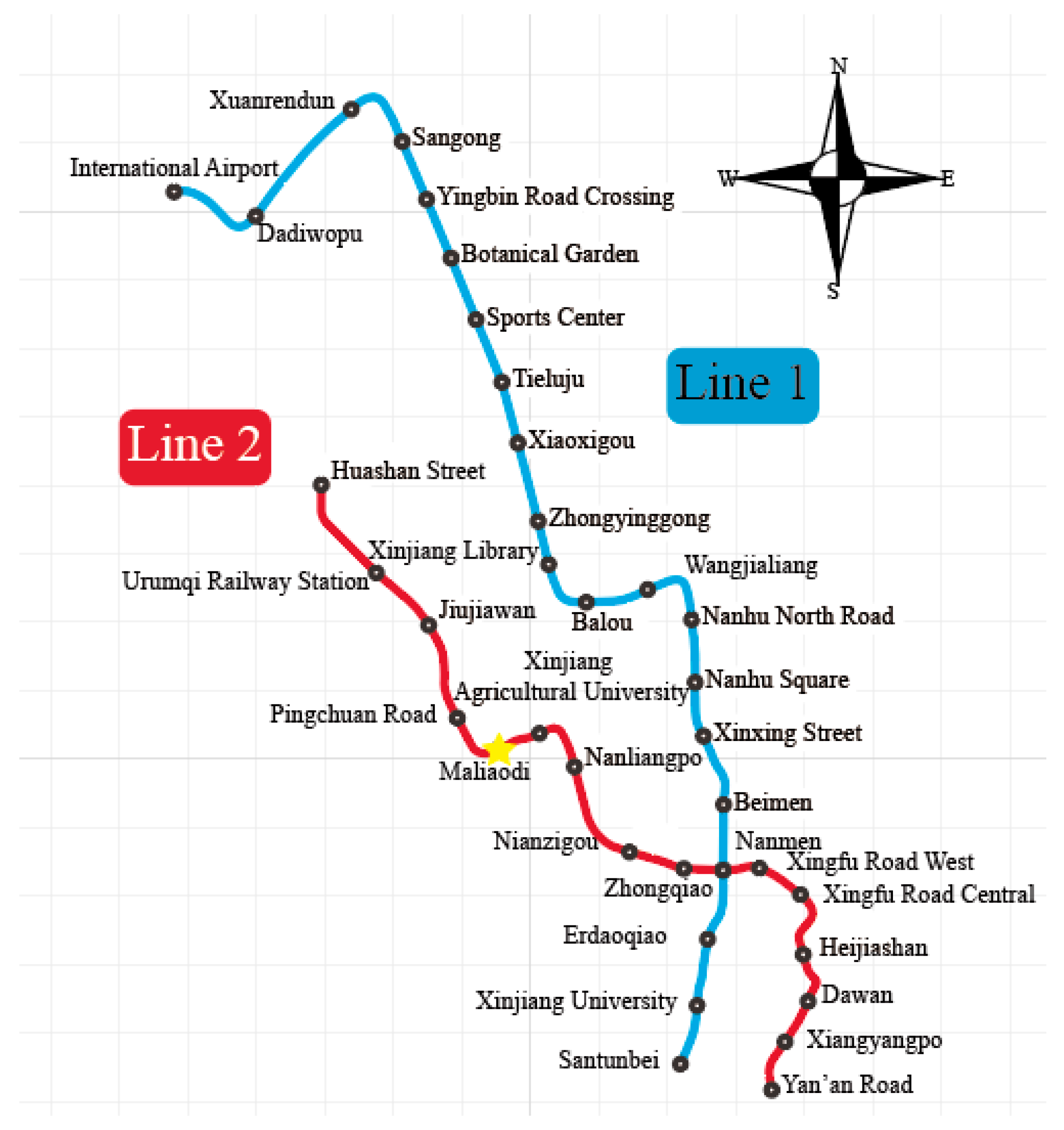
This work is based on the surface settlement monitored during the construction of the rail transit in Urumqi. Urumqi is the capital city of the Xinjiang Uygur Autonomous Region and the core area of the Belt and Road. The terrain is uneven, surrounded by mountains on three sides, high in the south and low in the north. The winter is cold and long, and the geological conditions are complex. Currently, as shown in Figure 4, there are two subway lines in Urumqi: an operating Metro Line 1 runs from north to south, with a total length of approximately 27.6 km and 21 stations, connecting multiple passenger flow gathering and dispersing points; the Metro Line 2 runs from east to west and has a total of 16 stations, including 4 transfer stations. The first phase of the Metro Line 2 project starts from Yan’an Road Station in the south and ends at Huashan Street Station in the north. The total length of the main line is 19.35 km, all of which is beneath the ground.

3.2. Data Source

The monitoring scope covers multiple areas, including surface subsidence and subsidence of underground pipelines such as underground, sewage, gas, water supply, and drainage pipelines around the main body of the station, the main line of the section, vertical shafts, and transverse passages. Based on the different excavation locations, depths, geological conditions, and support structures on site, monitoring was conducted at different frequencies to establish a settlement database for Urumqi Metro between 30 March 2014 and June 2023.

4. Result Analyses

4.1. Classification of Settlement Curves

4.1.1. Fluctuation Characteristics

Fluctuation characteristics describe the fluctuation trend in, shape of, and change in subway settlement curves, including three aspects: trend characteristics, statistical characteristics, and time domain characteristics. Through the extraction of key fluctuation characteristics in the settlement curve, the volatility of the settlement curve can be quantified, and different settlement curve categories can be clearly defined and distinguished.

Trend characteristics describe the overall trend in the subway settlement curve over time, including an upward trend, a downward trend, a stable trend, and an oscillating trend. An oscillating trend does not have an obvious periodicity or regularity, showing randomness and chaos. Statistical characteristics refer to the statistical properties and data distribution of the subway settlement curve data, including maximum value, minimum value, average value, variance, standard deviation, kurtosis, and root mean square value. Time domain characteristics are used to reveal the degree of fluctuation, skewness, and kurtosis of the subway settlement curve by analyzing the numerical fluctuation of the settlement data over time. The main parameters are crag factor $K$ (7), waveform factor $W$ (8), peak factor $C$ (9), pulse factor $I$ (10), and margin factor $L$ (11).

$$K={\displaystyle \frac{{\sum }_1^n\left[x\left(t\right)-\overline{x}\right]}{(n-1){\left\{\sqrt{\frac{1}{n-1}{{\sum }_1^n\left[x\left(t\right)-\overline{x}\right]}^2}\right\}}^4}}$$

(7)

$$W={\displaystyle \frac{\sqrt{\frac{1}{n}{\sum }_1^n{x}^2\left(t\right)}}{\overline{x}}}$$

(8)

$$C={\displaystyle \frac{\mathit{max}\left|x\left(t\right)\right|}{\sqrt{\frac{1}{n}{\sum }_1^n{x}^2\left(t\right)}}}$$

(9)

$$I={\displaystyle \frac{\mathit{max}\left|x\left(t\right)\right|}{\overline{x}}}$$

(10)

$$L={\displaystyle \frac{\mathit{max}\left|x\left(t\right)\right|}{{\left[\frac{1}{n}{\sum }_1^n\sqrt{\left|x\left(t\right)\right|}\right]}^2}}$$

(11)

4.1.2. Classification Results of Subway Settlement Curves

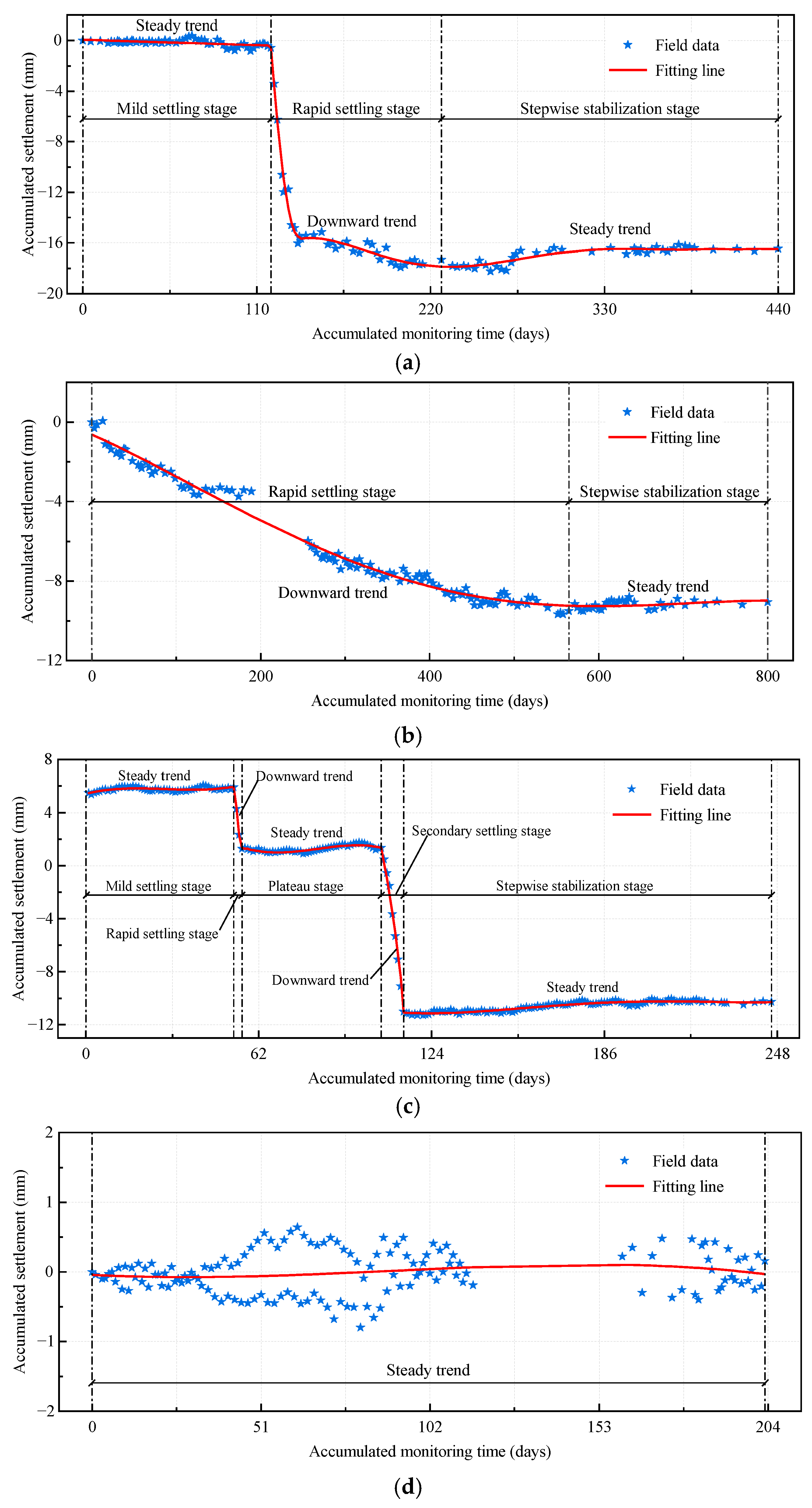
During metro construction, ground settlement manifests as a complex, high-dimensional, and nonlinear deformation process influenced by multiple factors. Settlement curves from different monitoring points exhibit diverse characteristics. Through systematic summarization and analysis of extensive settlement monitoring data from Urumqi Metro, quantitative analysis of fluctuation patterns and comparative validation revealed that these settlement curves can be categorized into five archetypal patterns. There are inverse cotangent curves, exponential curves, multi-step curves, one-shaped curves, and oscillating curves, as shown in Figure 5. Each curve type demonstrates distinctive fluctuation characteristics and evolutionary behaviors. Ultimately, a classification standard for settlement curves was established based on three key features: fluctuation trends, waveform factors, and kurtosis factors.

Figure 5a shows the inverse cotangent curve, whose fitting curves are shaped like inverse cotangent functions, and exhibit three-phase evolution: (1) initial mild settlement (stable trend with minor fluctuations), (2) rapid deformation (pronounced downward trend), and (3) asymptotic stabilization (negligible rate change post-construction). This characteristic may correspond to the gradual disturbance of strata during the initial construction phase, rapid deformation of strata during active construction operations, and progressive stabilization of strata in the final construction stage.

Figure 5b shows the exponential curve, whose fitted curves resemble the exponential function with the base greater than 0 and less than 1. The settling process demonstrates biphasic behavior: (1) accelerated settlement analogous to phase 2 of inverse cotangent-type, followed by (2) progressive stabilization matching phase 3 characteristics.

Figure 5c shows a multi-step curve, and its fitting curve presents the characteristics of multiple stage changes, consisting of several obvious step segments, with obvious jumps between different steps. The settlement process is displayed as a five-stage deformation: sequential transitions between (1) quiescent settlement (near-zero rate), (2) rapid deformation, (3) temporary plateau, (4) secondary settlement, and (5) final stabilization with slight rebound.

Figure 5d shows a one-line curve, which maintains stable deformation (±2 mm range) with gentle fluctuations, typically observed at distal monitoring points. This type of curve usually occurs in areas with relatively uniform geological conditions and weak construction impact.

Figure 5e is the oscillating-type curve, which presents aperiodic random fluctuations, suggesting multifactorial interference mechanisms.

4.1.3. Settlement Curve Classification Criteria

The classification of settlement curves is based on three key characteristics—fluctuation trend, waveform factor (WF), and crag factor (CF)—where the trend exhibits the strongest discriminative power while WF and CF vary across samples. The classification process involves (1) piecewise polynomial fitting to accommodate nonlinear deformation patterns, (2) deterministic categorization by comparing measured WF (≥0) and CF (≥0) against predefined thresholds, and (3) Fréchet distance minimization for ambiguous cases, ensuring robust pattern matching through geometric similarity assessment. Fluctuation characteristics of the five types of settling curves are shown in

Table 1. Results of fluctuation characteristics of five representative types of settlement curves.

Indicator Characteristics	Inverse Cotangent Curve	Exponential Curve	Multi-Step Curve	One-Shaped Curve	Oscillating Curve
Maximum Value/mm	0.062	−0.62	5.913	0.101	4.332
Minimum Value/mm	−17.87	−9.264	−11.137	−0.075	−1.345
Mean/mm	−9.295	−6.837	−3.876	−0.016	1.585
Variance	66.613	8.167	51.254	0.003	2.161
Standard Deviation	8.162	2.858	7.159	0.051	1.47
Root Mean Square	12.370	7.410	8.141	0.053	2.162
Peak/mm	17.932	8.644	17.049	0.176	5.676
Skewness	0.193	0.993	0.229	0.491	0.037
Waveform Factor	1.330	1.084	1.139	1.128	1.19
Peak Factor	0.005	−0.084	0.726	1.903	2.003
Pulse Factor	0.007	−0.091	0.827	2.147	2.383
Margin factor	0.01	−0.097	0.925	2.368	2.658
Cliff Factor	1.822	1.326	1.54	1.611	2.329
Trend Characteristics	Stable–decline–stable trend	Decline–stable trend	Stable–decline–stable–decline–stable trend	Stable trend	Damping trend

.

4.2. Selection of Optimal Module

The CI model is used to reduce the noise of five types of typical settlement curves; the correlation coefficients are all greater than 0.97, and the $RMSE$s are all less than 0.55, which indicates that the noise interference can be effectively reduced. This provides a more reliable database for settlement prediction.

All settlement monitoring records were organized chronologically according to the construction timeline, reflecting the inherently time-dependent and irreversible nature of the settlement process. To simulate a realistic forecasting scenario and strictly prevent data leakage, a temporal validation approach was adopted wherein the initial 87.5 percent of the data was used for model calibration and the subsequent 12.5 percent was reserved as a hold-out test set for performance evaluation. This partitioning ratio was informed by a previous study [25] and empirical validation. It ensures that the training set captures long-term evolutionary trends while the test set remains sufficiently large to permit a meaningful assessment of the model’s multi-step predictive accuracy. Through trial and error, the hyperparameters were set as shown below. In the AL model, the training step is set to 5, the prediction step is set to 1, the optimizer uses Adam’s algorithm, and $RMSE$ is used for the loss function. The GS model has ε ∈ [0, 2], C ∈ [0, 10], and G ∈ [0, 100]. The PB model has 2 nodes in the input layer, 5 nodes in the hidden layer, 1 node in the output layer, and 20 particle swarms for the number of particles. The rest of the parameters are shown in

Table 2. Parameter settings for each model.

Parameter	Inverse Cotangent Curve	Exponential Curve	Multi-Step Curve	One-Shaped Curve	Oscillating Curve
Sample size	132	146	230	144	115
ARIMA (p)	2	0	3	4	1
ARIMA (q)	1	1	1	0	1
ARIMA (d)	1	2	3	0	2
Number of training times for AL	750	800	1200	850	600
Number of particle swarm generations for GS	12	14	20	12	12
Number of particles per generation of GS	11	11	12	12	10
Optimal ε of GS	0.181	0.07	0.574	0.046	0.029
Optimal C of GS	7.929	8.707	2.015	9.065	4.775
Optimal G of GS	3.788	69.884	7.048	4.159	30.505
C1 = C2 of PB	2.05	1.85	2.45	1.9	2
Number of evolutions of PB	5	8	10	7	4
Maximum inertia weight of PB	0.9	0.8	0.9	0.7	0.8
Minimum inertia weight of PB	0.3	0.4	0.3	0.3	0.3

.

Different sequences have their own unique characteristics and patterns, so the most appropriate prediction model needs to be targeted. The distribution of prediction results and the absolute errors for the five types of sedimentation curves are shown in

Table 3. Evaluation results of predictions for five types of settlement curves.

Curve Categories	Predictive Models	$\mathit{R}\mathit{M}\mathit{S}\mathit{E}$	$\mathit{M}\mathit{A}\mathit{E}$	${\mathit{R}}^2$	$\mathit{M}\mathit{A}\mathit{P}\mathit{E}$ (%)
Inverse cotangent curve	ARIMA	0.0430	0.0461	0.9065	0.2794
	AM-LSTM	0.0174	0.0166	0.9888	0.1003
	GA-SVR	0.0895	0.0892	0.7016	0.5407
	PSO-BP	0.0610	0.0600	0.8616	0.3641
Exponential curve	ARIMA	0.0262	0.0214	0.9759	0.2324
	AM-LSTM	0.0396	0.0359	0.9630	0.3911
	GA-SVR	0.0756	0.0733	0.7994	0.8077
	PSO-BP	0.0719	0.0568	0.8186	0.6219
Multi-step curve	ARIMA	0.0844	0.0830	0.2232	0.8106
	AM-LSTM	0.0464	0.0439	0.7652	0.4295
	GA-SVR	0.0296	0.0282	0.9046	0.2765
	PSO-BP	0.0276	0.0230	0.9169	0.2255
One-shaped curve	ARIMA	0.0932	0.0731	0.8029	58.0732
	AM-LSTM	0.0349	0.0271	0.9725	27.3645
	GA-SVR	0.0238	0.0238	0.9871	24.1412
	PSO-BP	0.0991	0.0869	0.7775	85.0881
Oscillating curve	ARIMA	0.2729	0.2216	0.8485	24.7111
	AM-LSTM	0.3248	0.2461	0.7855	21.7981
	GA-SVR	0.0104	0.0099	0.9998	1.5953
	PSO-BP	0.1857	0.1542	0.9299	29.1099

and Figure 6. The absolute error of prediction can be calculated using $AE=\left|predictedvalue-measuredvalue\right|$.

In the prediction of the inverse cotangent curves, the AM-LSTM model performs the best, as shown in Figure 6a. With AE < 0.03 mm, the longitudinal region of the box is narrow, and the data is concentrated near the average value, with a small degree of dispersion and a relative error of less than 0.148%, an $RMSE$ = 0.0174 mm, an $MAE$ = 0.0166 mm, an $MAPE$ = 0.1003%, an $R^2$ = 0.9888, and excellent predictive performance. Therefore, the most suitable prediction model for the inverse cotangent curve is the AM-LSTM model.

In the prediction of exponential curves, the ARIMA model performs most prominently, as in Figure 6b. The relative error of prediction is less than 0.591%, with an $RMSE$ = 0.0262 mm, an $MAE$ = 0.0214 mm, an $MAPE$ = 0.2324%, and an $R^2$ = 0.9759. When AE < 0.06 mm, the data distribution is tight with the lowest mean, median, and plurality. However, the ARIMA model training time will be particularly long when the sample size is large. The AM-LSTM model, which is only second to the ARIMA model in terms of prediction effect, has a smaller difference in prediction effect, but the time is greatly reduced. Therefore, for exponential curves, the ARIMA model is suitable for small-sample data, and the AM-LSTM model is suitable for large-sample data.

In the multi-step curve prediction, the PSO-BP model stands out for its ability to adapt to the multi-step feature changes in the data, as shown in Figure 6c. The relative error of prediction is less than 0.557% with $RMSE$ = 0.0276 mm, $MAE$ = 0.0230 mm, $MAPE$ = 0.2255%, and $R^2$ = 0.9169. The AE is <0.06 mm, and the lower boundary of the box, the mean, the median, and the plurality are at the lowest position. Therefore, the optimal prediction model for the multi-step curve is the PSO-BP model.

The GA-SVR model performs best in the prediction of the oscillating curves, as in Figure 6d. The prediction results are $RMSE$ = 0.0238 mm, $MAE$ = 0.0238 mm, $MAPE$ = 24.1412%, and $R^2$ = 0.9871. With AE < 0.025 mm, the data of box plots are tightly centered around 0, and the prediction performance is the best. Therefore, the optimal prediction model for the oscillating curves is the GA-SVR model.

Among the oscillatory-type curves, the GA-SVR model performs the best, as shown in Figure 6e, and its ability to capture and predict the oscillatory features makes it optimal in all the metrics. Among them, the relative error is less than 4.826%, with an $RMSE$ = 0.0104 mm, an $MAE$ = 0.0099 mm, an $MAPE$ = 1.5953%, and an $R^2$ = 0.9998. The AE is <0.02 mm, which is tightly centered near 0. Therefore, the optimal prediction model for the oscillatory-type curve is also the GA-SVR model.

4.3. Validation of the Subway Settlement Layering Prediction Model

To evaluate the accuracy and stability of the subway settlement layering prediction model proposed in this study, its performance is tested using data from the newly excavated Maliaodi Station, as shown in Figure 4. Critically, this station represents a new, previously unseen case whose data was not involved in either the initial curve classification or the model training phases, ensuring an unbiased assessment of the framework’s performance. The geological conditions of Maliaodi Station are representative of Urumqi’s typical stratigraphy, comprising Quaternary Holocene artificial fill, Upper and Middle Pleistocene alluvial strata, and Jurassic mudstones, sandstones, and conglomerates. The groundwater table is shallow, and the site is surrounded by densely populated buildings, with a fracture zone to the west and a viaduct to the east, making it a complex and challenging construction environment.

In this study, monitoring site DB-09-07 at Maliaodi Station is selected as a case study, with a total monitoring duration of 792 days and 393 monitoring periods. The main module is first applied to preprocess the data, followed by the selective module for prediction. The predicted results are then validated by comparison with measured data to assess model performance.

4.3.1. Main Module Determination

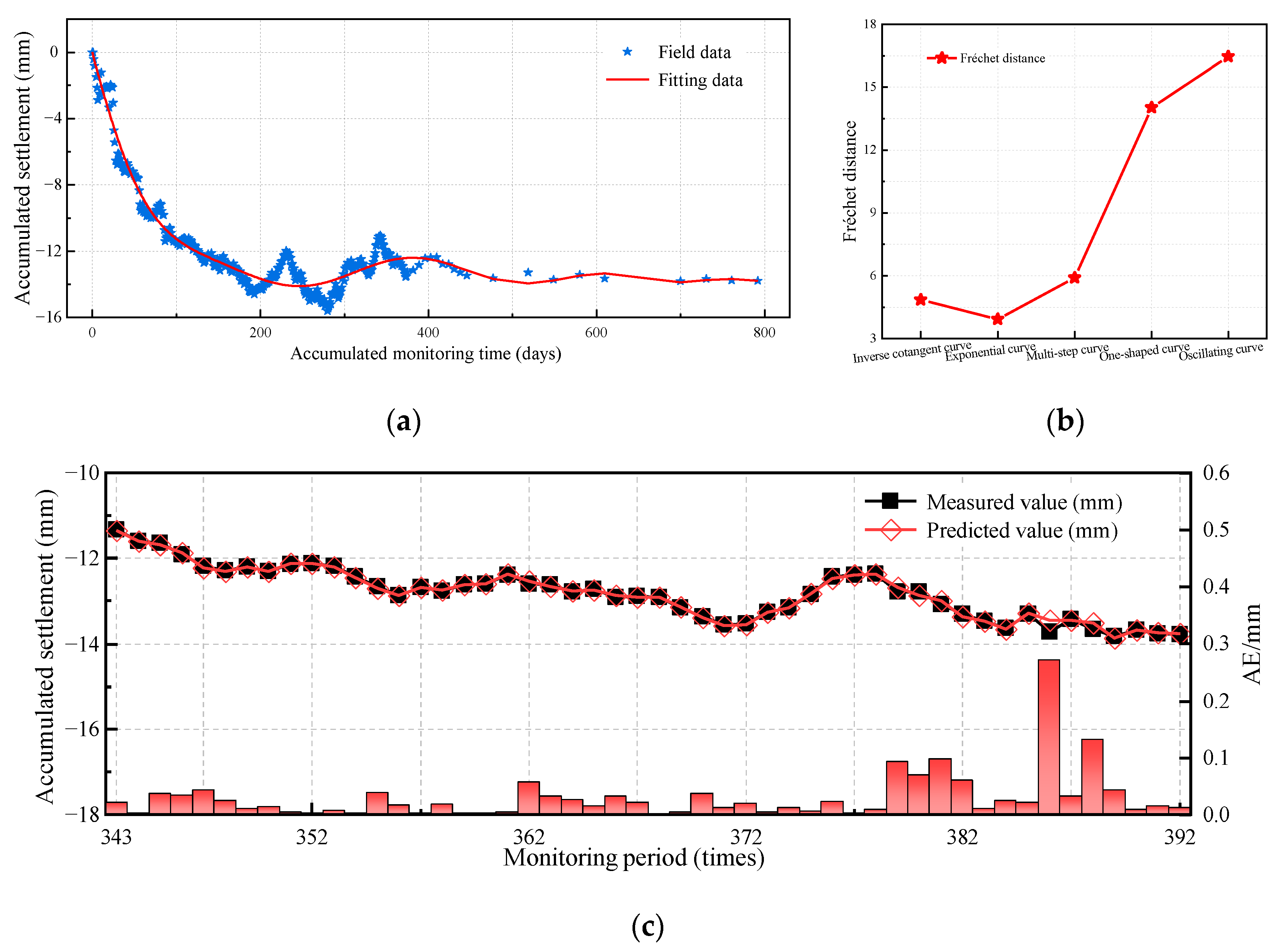
Data fitting was performed on the selected data from monitoring point DB-09-07, with the original data and the corresponding fitted curves presented in Figure 7a. Analysis of the fluctuation characteristics reveals that the fitted curve exhibits a downward-stable trend with slight mid-section fluctuations, a behavior similar to that of the exponential curve. The waveform factor is 3.15, and the crag factor is 0.001, both of which closely match those of the exponential curve, indicating that the curve belongs to the exponential type. For further verification, the Fréchet distances between the fitted curve and the five types of settlement curves were computed. As shown in Figure 7b, the smallest distance was observed with the exponential curve. These consistent findings confirm that the curve should be classified as exponential, thereby guiding its incorporation into the subway settlement hierarchical prediction model’s selective module for optimal prediction.

4.3.2. Selective Module Prediction

As stated in Section 4.3.1, the monitoring curve from point DB-09-07 is determined to be an exponential curve. With approximately 400 records, this dataset is considered relatively extensive within the domain of subway settlement monitoring. In comparative assessments, the AM-LSTM model demonstrates significantly superior performance over the ARIMA model in terms of both computational efficiency and predictive accuracy when handling large-sample data. Consequently, the AM-LSTM framework was selected for subsequent predictive modeling in this study. Firstly, the original observation signal is preprocessed, and then the AM-LSTM model is used for prediction, the number of training is 1500 times, the training step is five steps, the prediction step is one step, the selected optimizer is Adam’s algorithm, and the loss function of the prediction model is the $RMSE$ loss function; the prediction results are shown in Figure 7c. In addition, the AE is < 0.3 mm, with most values being concentrated in the range of 0.1 mm, and $RMSE$ = 0.0524 mm, $MAE$ = 0.0289 mm, $R^2$ = 0.9926, and $MAPE$ = 0.2217%, with high prediction accuracy.

5. Discussion

Settlement monitoring of the construction perimeter is crucial in underground space development and construction. In this paper, by analyzing the settlement data of the Urumqi subway, a hierarchical prediction method for subway settlement curves based on waveform features is proposed, which can more accurately capture and understand the complex relationship behind the data, reduce the prediction error, and significantly improve the prediction accuracy and efficiency.

By analyzing the settlement collation during the excavation of the Urumqi subway in this paper, there is a complex nonlinear relationship between settlement and many uncertain factors, and the surface settlement data from different monitoring points possess different characteristics. Therefore, a single algorithmic model cannot capture all the features hidden in the surface settlement data, and it is equally difficult to make accurate predictions with a single algorithmic model. This is consistent with the features found by Yagmur [22], Yan et al. [48], and Ding et al. [49]. In this paper, a hierarchical prediction model based on the waveform features of subway settlement curves is developed, which can better adapt to the prediction of subway settlement in different regions and overcome the limitations of single-model prediction. To further substantiate the inadequacy of traditional mathematical functions, we took the exponential-type curves as a test case and systematically fitted the monitored series with six families of closed-form functions: exponential, logarithmic, power, hyperbolic, logistic, and rational. The best performer among them—a rational function—achieved an $RMSE$ = 0.2336 mm, an $MAE$ = 0.2032 mm, and an $MAPE$ = 2.24%, which is significantly poorer than the $RMSE$ = 0.0262 mm and $MAPE$ = 0.232% delivered by the ARIMA/AM-LSTM models selected in our framework. This comparative exercise confirms that purely mathematical curve fitting cannot attain acceptable forecasting accuracy in complex engineering scenarios, thereby reinforcing the necessity of adopting machine learning strategies.

The prediction models required for different types of curves also have their own focuses, and the advantages and applicability of different models are also different, so choosing the suitable model according to the characteristics of the curve data is crucial for improving the prediction accuracy. Among the four types of prediction models, the AM-LSTM model can successfully capture the nonlinear changes in inverse coset and large-sample exponential curves; the ARIMA model, as a classical time series prediction method, can effectively capture the trend changes in small-sample exponential curves; the PSO-BP model is highly adaptive and can effectively deal with the sudden changes in the data, and it is suitable for predicting the multi-step curves with complex phase changes; and the GA-SVR model can effectively deal with irregular dynamic changes and can better capture the oscillatory trend characteristics of the oscillatory curve.

In addition, the rapid settling and gradual stabilization phases of the inverse one-shaped curve in this paper have some similarity with the fluctuation characteristics of the exponential curve. As a result, the exponential curve is regarded as a part of the settling process of the inverse one-shaped curve, which can be categorized as the same type of settling curve, and the prediction model is directly selected from the AM-LSTM model. When the cumulative settlement change in the inverse one-shaped curve, exponential curve, multi-step curve, and oscillatory curve is within the range of ±2 mm, all of them can be regarded as oscillating curves, and thus the oscillating curves can be categorized into any of these four types of curves. As shown in Figure 5d, the oscillating curves in this paper have no regular change without considering the amplitude, which is in line with the characteristics of oscillatory curves, and the optimal prediction model is exactly the optimal prediction model for oscillatory curves.

On the other hand, different factors such as geological conditions, construction methods, and monitoring techniques can directly affect the settlement profile. The prediction method in this paper performs well on Urumqi Metro data, but its universal applicability needs to be validated in more areas and environments.

6. Conclusions and Outlook

Based on the settlement monitoring data from the Urumqi subway system, this paper proposes a hierarchical prediction model that integrates a main module and a selective module. The main module, developed by quantifying the waveform characteristics of subway settlement curves, enables the classification of monitoring curves into five categories: inverse cotangent curves, exponential curves, multi-step curves, one-shaped curves, and oscillating curves. The selective module employs multiple prediction models to determine the optimal model for each curve type. Finally, case studies are conducted to verify the method’s effectiveness. The primary research conclusions are as follows.

(1) By quantifying the waveform characteristics, the main module categorizes subway settlement curves into the five aforementioned types, thereby establishing a classification system based on their fluctuating characteristics.

(2) The five types of typical subway settlement curves are predicted using the ARIMA model, AM-LSTM model, GA-SVR model, and PSO-BP model to establish the selective module. When comparing the prediction values and prediction effects of various types of curves, it can be obtained that the most suitable prediction model for the inverse cotangent curve is the AM-LSTM model. The most suitable prediction models for exponential curves are the ARIMA model (small data) and the AM-LSTM model (large data). The most suitable prediction model for multi-step curves is the PSO-BP model. The most appropriate prediction model for one-shaped curves and oscillating curves is the GA-SVR model.

(3) The newly excavated lot data of the Urumqi subway is used to verify the prediction model of this paper as an example, and the prediction accuracy is very high. The results can be applied to the future construction of the Urumqi subway, which has strong engineering significance.

This study provides a novel perspective and methodology for the classification and intelligent prediction of subway settlement curves, significantly enhancing prediction accuracy and efficiency. Future research should explore additional predictive models and develop hybrid or ensemble learning approaches, such as hierarchical clustering [50,51], to address the challenges posed by diverse settlement curve types across varying environments.

References

1. Yang, W.; Hu, Y.; Hu, C.; Yang, M. An Agent-Based Simulation of Deep Foundation Pit Emergency Evacuation Modeling in the Presence of Collapse Disaster. Symmetry 2018, 10, 581. [Google Scholar] [CrossRef]
2. Liu, L.; Wu, R.; Congress, S.S.C.; Du, Q.; Cai, G.; Li, Z. Design Optimization of the Soil Nail Wall-Retaining Pile-Anchor Cable Supporting System in a Large-Scale Deep Foundation Pit. Acta Geotech. 2021, 16, 2251–2274. [Google Scholar]
3. Ma, B.; Xiao, Y.; Lan, T.; Zhang, C.; Wang, Z.; Xiang, Z.; Li, Y.; Zhao, Z. Predicting Soft Soil Settlement with a FAGSO-BP Neural Network Model. Buildings 2025, 15, 1343. [Google Scholar] [CrossRef]
4. Su, J.; Wang, Y.; Niu, X.; Sha, S.; Yu, J. Prediction of Ground Surface Settlement by Shield Tunneling Using XGBoost and Bayesian Optimization. Eng. Appl. Artif. Intell. 2022, 114, 105020. [Google Scholar] [CrossRef]
5. Zhang, J.; Jiang, H.; Wang, J.; Feng, J. A Model Based on Neural Network to Predict Surface Settlement During Subway Station Construction: A Case Study of the Dongba-Zhongjie Station in Beijing, China. Buildings 2025, 15, 1823. [Google Scholar] [CrossRef]
6. Hwang, R.N.; Moh, Z.-C. Prediction of Long-Term Settlements Induced by Shield Tunneling. J. Geoengin. 2006, 1, 63–70. [Google Scholar]
7. Feng, S.; Liu, J. Deformation Monitoring and Control of Geotechnical Engineering Based on Intelligent Optimal Algorithms. In Proceedings of the 2019 11th International Conference on Measuring Technology and Mechatronics Automation (ICMTMA), Qiqihar, China, 28–29 April 2019; IEEE: New York, NY, USA, 2019; pp. 341–344. [Google Scholar]
8. Wang, F.; Du, X.; Li, P. Predictions of Ground Surface Settlement for Shield Tunnels in Sandy Cobble Stratum Based on Stochastic Medium Theory and Empirical Formulas. Undergr. Space 2023, 11, 189–203. [Google Scholar] [CrossRef]
9. Zhong, K.; Ma, J.; Han, M. Online Prediction of Noisy Time Series: Dynamic Adaptive Sparse Kernel Recursive Least Squares from Sparse and Adaptive Tracking Perspective. Eng. Appl. Artif. Intell. 2020, 91, 103547. [Google Scholar] [CrossRef]
10. Hu, L.; Kasama, K.; Wang, G.; Takahashi, A. Assessing the Influence of Geotechnical Uncertainty on Existing Tunnel Settlement Caused by New Tunneling Underneath. Tunn. Undergr. Space Technol. 2025, 155, 106189. [Google Scholar] [CrossRef]
11. Kim, D.; Kwon, K.; Pham, K.; Oh, J.-Y.; Choi, H. Surface Settlement Prediction for Urban Tunneling Using Machine Learning Algorithms with Bayesian Optimization. Autom. Constr. 2022, 140, 104331. [Google Scholar] [CrossRef]
12. Zhou, Z.; Ding, H.; Miao, L.; Gong, C. Predictive Model for the Surface Settlement Caused by the Excavation of Twin Tunnels. Tunn. Undergr. Space Technol. 2021, 114, 104014. [Google Scholar] [CrossRef]
13. Moon, J.; Hossain, M.B.; Chon, K.H. AR and ARMA Model Order Selection for Time-Series Modeling with ImageNet Classification. Signal Process. 2021, 183, 108026. [Google Scholar] [CrossRef]
14. Cao, L.; Chen, X.; Lu, D.; Zhang, D.; Su, D. Theoretical Prediction of Ground Settlements Due to Shield Tunneling in Multi-Layered Soils Considering Process Parameters. Undergr. Space 2024, 16, 29–43. [Google Scholar] [CrossRef]
15. Li, C.; Li, J.; Shi, Z.; Li, L.; Li, M.; Jin, D.; Dong, G. Prediction of Surface Settlement Induced by Large-Diameter Shield Tunneling Based on Machine-Learning Algorithms. Geofluids 2022, 2022, 4174768. [Google Scholar] [CrossRef]
16. Zhang, W.; Zhang, R.; Wu, C.; Goh, A.T.C.; Lacasse, S.; Liu, Z.; Liu, H. State-of-the-Art Review of Soft Computing Applications in Underground Excavations. Geosci. Front. 2020, 11, 1095–1106. [Google Scholar] [CrossRef]
17. Lu, D.; Xu, B.; Kong, F.; Ma, Y. Intelligent Prediction Method for Settlement Curves of Shield Tunnel Based on Machine Learning Algorithms. J. Beijing Univ. Technol. 2024, 50, 1285–1300. [Google Scholar] [CrossRef]
18. Casado-Vara, R.; Martin Del Rey, A.; Pérez-Palau, D.; de-la-Fuente-Valentín, L.; Corchado, J.M. Web Traffic Time Series Forecasting Using LSTM Neural Networks with Distributed Asynchronous Training. Mathematics 2021, 9, 421. [Google Scholar] [CrossRef]
19. Noor, F.; Haq, S.; Rakib, M.; Ahmed, T.; Jamal, Z.; Siam, Z.S.; Hasan, R.T.; Adnan, M.S.G.; Dewan, A.; Rahman, R.M. Water Level Forecasting Using Spatiotemporal Attention-Based Long Short-Term Memory Network. Water 2022, 14, 612. [Google Scholar] [CrossRef]
20. Sun, J.; Yuan, J. Soil Disturbance and Ground Movement under Shield Tunnelling and Its Intelligent Prediction by Using ANN Technology. Chin. J. Geotech. Eng. 2001, 23, 261–267. [Google Scholar]
21. Li, P.P.; Li, J.P.; Liu, G.Y.; Zhou, P. Prediction of Dredged Soil Settlement Based on Improved BP Neural Network. IOP Conf. Ser. Earth Environ. Sci. 2024, 1337, 012013. [Google Scholar] [CrossRef]
22. Yagmur, N.; Musaoglu, N. The Comparison of ARIMA and LSTM in Forecasting of Long-Term Surface Movements Derived from PSINSAR. In Proceedings of the Earth Observing Systems XXVIII, San Diego, CA, USA, 20–25 August 2023; p. 31. [Google Scholar]
23. Cui, Z.-D.; Hua, S.-S.; Yan, J.-S. Long-Term Settlement of Subway Tunnel and Prediction of Settlement Trough in Coastal City Shanghai. In Proceedings of the GeoShanghai 2018 International Conference: Multi-physics Processes in Soil Mechanics and Advances in Geotechnical Testing, Shanghai, China, 27–30 May 2018; Hu, L., Gu, X., Tao, J., Zhou, A., Eds.; Springer: Singapore, 2018; pp. 458–467, ISBN 978-981-13-0094-3. [Google Scholar]
24. Bao, X.; Zhang, R.; Shama, A.; Li, S.; Xie, L.; Lv, J.; Fu, Y.; Wu, R.; Liu, G. Ground Deformation Pattern Analysis and Evolution Prediction of Shanghai Pudong International Airport Based on PSI Long Time Series Observations. Remote Sens. 2022, 14, 610. [Google Scholar] [CrossRef]
25. Zhu, S.; Qin, Y.; Meng, X.; Xie, L.; Zhang, Y.; Yuan, Y. Prediction Model of Land Surface Settlement Deformation Based on Improved LSTM Method: CEEMDAN-ICA-AM-LSTM (CIAL) Prediction Model. PLoS ONE 2024, 19, e0298524. [Google Scholar] [CrossRef] [PubMed]
26. Qiu, P.; Liu, F.; Zhang, J. Land Subsidence Prediction Model Based on the Long Short-Term Memory Neural Network Optimized Using the Sparrow Search Algorithm. Appl. Sci. 2023, 13, 11156. [Google Scholar] [CrossRef]
27. Zhang, W.-S.; Yuan, Y.; Long, M.; Yao, R.-H.; Jia, L.; Liu, M. Prediction of Surface Settlement around Subway Foundation Pits Based on Spatiotemporal Characteristics and Deep Learning Models. Comput. Geotech. 2024, 168, 106149. [Google Scholar] [CrossRef]
28. Fréchet, M. Sur Quelques Points Du Calcul Fonctionnel. Rend. Circ. Matem. Palermo 1906, 22, 1–72. [Google Scholar] [CrossRef]
29. Eiter, T.; Mannila, H. Computing Discrete Fréchet Distance. 1994. Available online: https://api.semanticscholar.org/CorpusID:16010565 (accessed on 15 September 2025).
30. Gudmundsson, J.; Van Renssen, A.; Saeidi, Z.; Wong, S. Translation Invariant Fréchet Distance Queries. Algorithmica 2021, 83, 3514–3533. [Google Scholar] [CrossRef]
31. Weise, J.; Mostaghim, S. Many-Objective Pathfinding Based on Fréchet Similarity Metric. In Evolutionary Multi-Criterion Optimization; Ishibuchi, H., Zhang, Q., Cheng, R., Li, K., Li, H., Wang, H., Zhou, A., Eds.; Lecture Notes in Computer Science; Springer International Publishing: Cham, Switzerland, 2021; Volume 12654, pp. 375–386. ISBN 978-3-030-72061-2. [Google Scholar]
32. Luo, Z.; Hasanipanah, M.; Bakhshandeh Amnieh, H.; Brindhadevi, K.; Tahir, M.M. GA-SVR: A Novel Hybrid Data-Driven Model to Simulate Vertical Load Capacity of Driven Piles. Eng. Comput. 2021, 37, 823–831. [Google Scholar] [CrossRef]
33. Cai, H.; Wang, Y.; Song, C.; Wang, T.; Shen, Y. Prediction of Surface Subsidence Based on PSO-BP Neural Network. J. Phys. Conf. Ser. 2022, 2400, 012046. [Google Scholar] [CrossRef]
34. Duan, C.; Hu, M.; Zhang, H. Comparison of ARIMA and LSTM in Predicting Structural Deformation of Tunnels during Operation Period. Data 2023, 8, 104. [Google Scholar] [CrossRef]
35. Yang, H.; Yue, J.; Zhou, Q. Dam Deformation Prediction Using SVM and ARIMA Combined Model. Bull. Surv. Mapp. 2021, 13, 5160. [Google Scholar] [CrossRef]
36. Zhang, T.; Wang, Z. Improve the LSTM Trajectory Prediction Accuracy through an Attention Mechanism. In Proceedings of the 2022 IEEE Transportation Electrification Conference & Expo (ITEC), Anaheim, CA, USA, 15–17 June 2022; IEEE: New York, NY, USA, 2022; pp. 190–195. [Google Scholar]
37. Yuan, Y.; Zhang, D.; Cui, J.; Zeng, T.; Zhang, G.; Zhou, W.; Wang, J.; Chen, F.; Guo, J.; Chen, Z.; et al. Land Subsidence Prediction in Zhengzhou’s Main Urban Area Using the GTWR and LSTM Models Combined with the Attention Mechanism. Sci. Total Environ. 2024, 907, 167482. [Google Scholar] [CrossRef]
38. Guo, S.; Lin, Y.; Feng, N.; Song, C.; Wan, H. Attention Based Spatial-Temporal Graph Convolutional Networks for Traffic Flow Forecasting. In Proceedings of the AAAI Conference on Artificial Intelligence, Honolulu, HI, USA, 27 January–1 February 2019; Volume 33, pp. 922–929. [Google Scholar]
39. Han, Y.; Li, Z.; Hu, X.; Wang, Y.; Geng, Z. Novel Long Short-Term Memory Model Based on the Attention Mechanism for the Leakage Detection of Water Supply Processes. IEEE Trans. Syst. Man Cybern Syst. 2024, 54, 2786–2796. [Google Scholar] [CrossRef]
40. Bharathi, A.; Sanku, R.; Sridevi, M.; Manusubramanian, S.; Chandar, S.K. Real-Time Human Action Prediction Using Pose Estimation with Attention-Based LSTM Network. SIViP 2024, 18, 3255–3264. [Google Scholar] [CrossRef]
41. Vapnik, V.N.; Vapnik, V. Statistical Learning Theory; John Wiley & Sons: Chichester, UK, 1998. [Google Scholar]
42. Feng, X.-T.; Zhao, H.; Li, S. Modeling Non-Linear Displacement Time Series of Geo-Materials Using Evolutionary Support Vector Machines. Int. J. Rock Mech. Min. Sci. 2004, 41, 1087–1107. [Google Scholar] [CrossRef]
43. Cai, W.; Wen, X.; Li, C.; Shao, J.; Xu, J. Predicting the Energy Consumption in Buildings Using the Optimized Support Vector Regression Model. Energy 2023, 273, 127188. [Google Scholar] [CrossRef]
44. Huang, Z.; Huang, J.; Zhang, J.; Li, X.; Zheng, H.; Liu, X. The Collapse Deformation Control of Granite Residual Soil in Tunnel Surrounding Rock: A Case Study. KSCE J. Civ. Eng. 2024, 28, 2034–2052. [Google Scholar] [CrossRef]
45. Jiang, C.-S.; Chen, X.; Jiang, B.-Y.; Liang, G.-Q. Hybrid Genetic Algorithm and Support Vector Regression for Predicting the Shear Capacity of Recycled Aggregate Concrete Beam. Soft Comput 2024, 28, 1023–1039. [Google Scholar] [CrossRef]
46. Yu, B.; Li, Q.; Zhao, T. Deformation Extent Prediction of Roadway Roof during Non-Support Period Using Support Vector Regression Combined with Swarm Intelligent Bionic Optimization Algorithms. Tunn. Undergr. Space Technol. 2024, 145, 105585. [Google Scholar] [CrossRef]
47. Li, X.; Jia, C.; Zhu, X.; Zhao, H.; Gao, J. Investigation on the Deformation Mechanism of the Full-Section Tunnel Excavation in the Complex Geological Environment Based on the PSO-BP Neural Network. Env. Earth Sci 2023, 82, 326. [Google Scholar] [CrossRef]
48. Yan, K.; Dai, Y.; Xu, M.; Mo, Y. Tunnel Surface Settlement Forecasting with Ensemble Learning. Sustainability 2019, 12, 232. [Google Scholar] [CrossRef]
49. Ding, Y.; Hang, D.; Wei, Y.-J.; Zhang, X.-L.; Ma, S.-Y.; Liu, Z.-X.; Zhou, S.-X.; Han, Z. Settlement Prediction of Existing Metro Induced by New Metro Construction with Machine Learning Based on SHM Data: A Comparative Study. J. Civ. Struct. Health Monit. 2023, 13, 1447–1457. [Google Scholar] [CrossRef]
50. Huang, X.; Han, M.; Deng, Y. A Hybrid GAN-Inception Deep Learning Approach for Enhanced Coordinate-Based Acoustic Emission Source Localization. Appl. Sci. 2024, 14, 8811. [Google Scholar] [CrossRef]
51. Sapidis, G.M.; Naoum, M.C.; Papadopoulos, N.A.; Golias, E.; Karayannis, C.G.; Chalioris, C.E. A Novel Approach to Monitoring the Performance of Carbon-Fiber-Reinforced Polymer Retrofitting in Reinforced Concrete Beam–Column Joints. Appl. Sci. 2024, 14, 9173. [Google Scholar] [CrossRef]
Figure 1. Layered prediction model of subway settlement.
Buildings 15 03390 g001
Figure 3. Word frequency statistics of papers related to subway settlement prediction from 2021 to 2025. (a) Word frequency cloud map. (b) Word frequency statistics chart.
Buildings 15 03390 g003
Figure 4. The Urumqi Metro Line map.
Buildings 15 03390 g004
Figure 5. Fluctuation characteristics of five types of settlement curves: (a) characteristics of inverse cotangent curve, (b) characteristics of exponential curve, (c) characteristics of multi-step curve, (d) characteristics of one-shaped curve, and (e) characteristics of oscillating curve.
Buildings 15 03390 g005aBuildings 15 03390 g005b
Figure 6. Prediction results of five types of settlement curves: (a) prediction results for inverse cotangent curve, (b) prediction results for exponential curve, (c) prediction results for multi-step curve, (d) prediction results for one-shaped curve, and (e) prediction results for oscillating curve.
Buildings 15 03390 g006
Figure 7. Case study of measuring point DB-09-07: (a) fitting results for DB-09-07, (b) Fréchet distance, and (c) forecast results for DB-09-07.
Buildings 15 03390 g007