A Hybrid Prediction Model for Wind–Solar Power Generation with Hyperparameter Optimization and Application in Building Heating Systems

Abstract

Accurate prediction of photovoltaic and wind power generation is essential for maintaining stable energy supply in integrated energy systems. However, the strong stochasticity and complex fluctuations in these energy sources pose significant challenges to forecasting. Traditional methods often fail to handle the non-stationary characteristics of the generation series effectively. To address this, we propose a novel hybrid prediction framework that integrates variational mode decomposition, the Pearson correlation coefficient, and a benchmark prediction model. Experimental results demonstrate the outstanding performance of the proposed method, achieving an R² value exceeding 0.995 along with minimal MAE and RMSE. The approach effectively mitigates hysteresis issues during prediction. Furthermore, the model shows strong adaptability; even when substituting different benchmark models, it maintains an R² above 0.99. When applied in a building heating system, accurate predictions help reduce indoor temperature fluctuations, enhance energy supply stability, and lower energy consumption, highlighting its practical value for improving energy efficiency and operational reliability.

1. Introduction

Currently, global energy consumption is still predominantly reliant on traditional energy sources, and by 2019, renewable energy had accounted for just over 20% of global electricity generation [1]. While the utilization of traditional energy sources generated significant economic income for nations, it simultaneously posed challenges such as environmental pollution. The extensive development and utilization of fossil fuels emit substantial amounts of harmful gases, including sulfur dioxide (SO₂), nitrogen oxides (NO_x), soot, and other pollutants, which adversely impact the natural environment and contribute to environmental degradation [2,3]. Given the escalating issue of global warming, people are endeavoring to reduce conventional energy consumption by embracing renewable energy sources, which are environmentally friendly and sustainable compared with traditional energy sources. Moreover, renewable energy can foster job creation and further economic development [4]. As the world’s energy transition deepens, the significance of renewable energy has grown, and various forms of renewable energy, including solar, geothermal, wind, and biomass energy, have become an integral part of the global energy supply system [5].

To address the global energy crisis, mitigate climate change, and minimize air pollution, countries worldwide are actively investing in the development and utilization of renewable energy [6]. Currently, research in renewable energy primarily focuses on wind, solar, biomass, geothermal, and nuclear energy, with photovoltaic and wind power generation being the most prominent [7]. Notably, solar and wind energy, due to their renewability and environmental friendliness, have garnered significant attention globally [8]. Wind and solar power generation are highly influenced by natural environmental factors, exhibiting strong randomness, volatility, and discontinuity. These characteristics result in unstable power generation, which in turn seriously affects the stability of grid operation. This further impacts the operation of the integrated energy system, hinders the development of effective scheduling plans, and ultimately reduces the reliability of energy supply within the integrated energy system [9,10]. Achieving effective use of renewable energy sources, realizing the coupling and complementarity between wind and solar energy, and developing a low-carbon integrated energy system are effective ways to address energy problems [11]. In order to solve these problems, predicting. the power generation of photovoltaic and wind power is one of the most effective methods to improve the efficiency of renewable energy utilization and ensure the stability of power supply [12]. Currently, wind and photovoltaic power generation prediction methods are mainly classified into three categories: physical prediction, statistical prediction, and machine learning, with physical prediction methods requiring an understanding of the laws of physics [13]. Because of the need to understand the detailed underlying principles of physical prediction methods, these principles can be complex. If equipment and human errors lead to inaccurate parameter measurements, this will directly reduce the performance of the entire model. In addition, the complex physical modeling process, slow computation speed, parameter inaccuracy, and other disadvantages may also cause certain prediction biases [14]. Statistical prediction methods primarily predict power by analyzing the evolutionary patterns of historical data. However, this method is not adept at capturing the inherent uncertainty of wind and photovoltaic power generation, which is marked by nonlinear dynamics [13]. With the advancements in artificial intelligence technology, machine learning methods have proven effective in extracting nonlinear and irregular features, demonstrating remarkable performance in predicting photovoltaic and wind power generation [15]. Commonly used machine learning methods include regression trees, support vector machines and artificial neural networks [16]. Among these, random forests (RFs) [17], BP neural networks [18] and support vector machines (SVMs) [19] have excellent predictive capabilities in the renewable energy sector. Nevertheless, a standalone machine learning model may suffer from overfitting and low convergence rates, while traditional shallow models rely on predefined nonlinear structures that are unable to delve into the deeper features of the data, thereby limiting the enhancement of prediction accuracy [20,21].

Due to the limitations of single prediction models in handling complex linear and nonlinear problems, their predictive performance tends to be unstable. Therefore, combined models integrating multiple algorithms are often employed for forecasting. By leveraging the strengths of different techniques, such hybrid approaches compensate for the limitations of single models, ultimately constructing a method that demonstrates greater robustness and accuracy. For instance, data preprocessing algorithms are combined with optimization algorithms. Additionally, the prediction of photovoltaic and wind power (WP) often involves utilizing variational modal decomposition (VMD) to disaggregate the data, followed by the performance of power prediction [22,23]. For example, Liu et al. employed the VMD method to decompose historical data during the prediction process and integrated it with a hybrid prediction model to predict solar radiation intensity. Their results demonstrated that VMD effectively addressed issues of high noise and volatility in the data, ultimately enhancing the model’s prediction accuracy [24]. Similarly, Wang et al. utilized VMD for data processing and adopted a context-embedded causal convolutional transformer (CCTrans) structure to predict subsequences. The accuracy and generalization of their model were validated through real-world cases [25]. Some studies used VMD to decompose the eigenvalues of predictor variables, for instance, Liu et al. constructed a hybrid prediction model for photovoltaic power generation, utilizing VMD to decompose the most relevant eigenvariables for model training. This approach enabled the mining of spatio-temporal characteristics from the data, and the results indicated that the model could serve as a reliable reference for grid operation and planning [26].

As can be seen above, VMD can effectively address issues such as modal aliasing. To achieve better prediction results, it is crucial to select an appropriate number of decomposed modes and penalty factors [27]. For instance, Li et al. employed a genetic algorithm to optimize the hyperparameters of VMD and experimentally demonstrated that this optimization could better manage the data [28]. Similarly, Li et al. utilized an artificial hummingbird algorithm to optimize VMD’s hyperparameters, confirming that different datasets require tailored hyperparameters to yield decomposition results suitable for the current data [29]. However, the aforementioned studies solely focused on optimizing VMD’s hyperparameters and predicting its intrinsic mode function (IMF), neglecting the potential relationship between these components and weather parameters. However, the aforementioned studies generally suffer from two shortcomings: On the one hand, they employ a single-algorithm approach to optimize the hyperparameters of VMD without designing tailored optimization objectives that account for the intermittent and discontinuous nature of wind and solar power generation. On the other hand, most of the IMF obtained from VMD are directly used for prediction without undergoing correlation analysis to filter out the IMF most critical to forecasting and least correlated with the original data. This results in subsequent models still being affected by noise and irrelevant information. These limitations constrain the improvement in prediction accuracy for wind and solar power generation.

Current research primarily focuses on optimizing the penalty factor and the number of modes in VMD through algorithmic approaches, while neglecting the correlation between the IMFs derived from VMD and meteorological parameters. The frequency characteristics of IMFs are directly influenced by meteorological conditions, and ignoring this correlation results in the loss of critical predictive information. Existing hybrid models merely achieve a simplistic “decomposition + prediction” combination without filtering redundant IMFs through correlation analysis or optimizing the parameters of the prediction models, leading to insufficient accuracy and generalization capability. Moreover, current studies mainly concentrate on improving prediction accuracy without integrating the prediction results with practical energy systems. Factors such as indoor temperature fluctuations and energy consumption control during heating seasons require a stable supply from wind and solar power generation. The neglect of combining prediction with real-world applications confines the research to a theoretical stage.

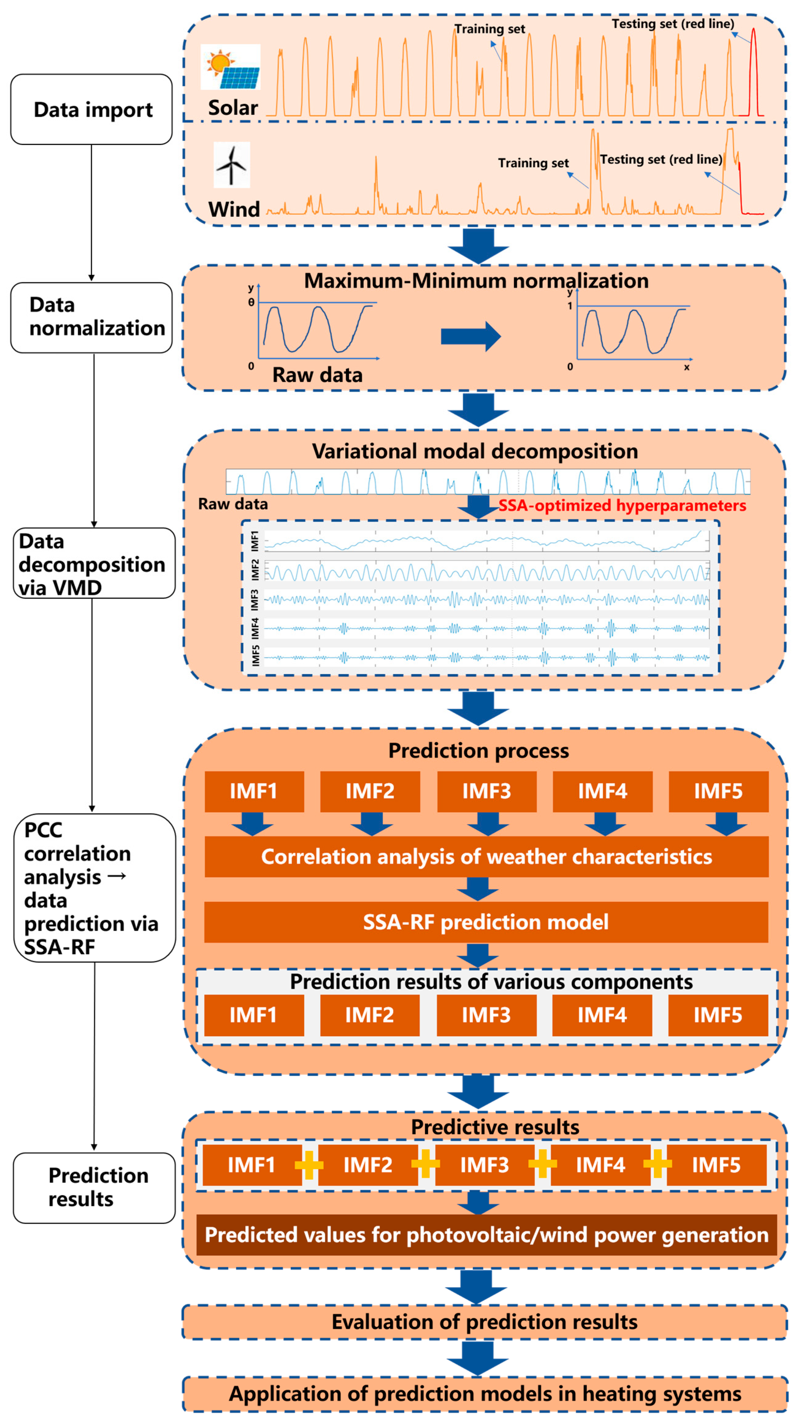
Therefore, this study investigates the correlation between the raw data and the IMF of power generation to elucidate the significance of weather characteristic parameters in predicting the IMF of power generation. Firstly, this study verified the accuracy of the power generation data and weather parameters. Subsequently, the dataset was normalized, and the Pearson correlation coefficient method (PCC) was employed to test the correlation between raw data and IMF variables. Finally, the Sparrow Search Algorithm (SSA) was used to optimize the random forest (RF) model for predicting the IMF of photovoltaic and wind power generation. This article performed predictions for some IMFs both with and without the inclusion of weather characteristic parameters and compared the prediction performance to demonstrate the effectiveness of the prediction method. Next, a brief description of the main contributions of this paper are as follows:

• A hybrid prediction framework was constructed: Most current hybrid prediction models adopt a “decomposition + prediction” approach without processing the decomposed IMF. Therefore, this study proposes a novel framework that innovatively integrates VMD, SSA, PCC, and prediction models. This framework is specifically designed to address issues such as intermittency and discontinuity in wind–solar power generation. The key finding is that IMFs with the weakest correlation to the original data contain insufficient feature information and must be predicted in conjunction with meteorological parameters to achieve high accuracy.
• Benchmark model and prediction performance validation: This study experimentally demonstrates that the proposed VMD-PCC framework is highly adaptable and does not rely on specific prediction models, fully illustrating that the proposed prediction framework possesses generalizability and robustness while delivering high-precision prediction performance.
• Practical application of the prediction model: A key contribution of this study lies in applying the prediction model to the operation of building energy systems, simulating a building heating system powered by wind–solar generation. The results show that the high-precision predictions of the proposed hybrid method significantly reduce indoor temperature fluctuations, lower energy consumption, and enhance comfort and operational stability.
• Resolution of the hysteresis issue in prediction: A common problem in renewable energy forecasting is the hysteresis in prediction curves. The hybrid prediction method proposed in this study effectively mitigates this hysteresis phenomenon. The results indicate that the model’s prediction curves closely align with the actual data at extreme points and during rapid changes.

2. Methods

2.1. Multi-Model Fusion Approach for Prediction

Based on SSA, PCC, VMD, and RF, this study proposes a hybrid prediction method for wind and photovoltaic power generation (VMD-PCC-SSA-RF). The prediction model is applied to a heating system to explore the impact of the model’s prediction accuracy on indoor temperature changes. The flowchart of this method is shown in Figure 1:

(1)

Select 20 days of photovoltaic/wind power generation data as experimental data. In this study, data from the first 19 days are used as the training set to train the model, while data from the 20th day are used as the test set.

(2)

Normalize the historical dataset of photovoltaic/wind power generation and fill in missing values to facilitate the subsequent prediction task.

(3)

Choose the minimum envelope entropy as the fitness function, which can characterize the sparse properties of different component signals. Then, the SSA performs an optimization search on the parameters of VMD (modal component K and penalty factor α). Input the optimal solution for modal component K and penalty factor α into VMD for data decomposition. The data is decomposed into K IMFs, with each IMF having distinct features and frequencies.

(4)

Utilize PCC to analyze the correlation between IMFs and raw data.

(5)

Predict the IMFs screened by PCC in conjunction with weather characteristic parameters, while performing time series prediction for the remaining IMFs. Combine these predictions to obtain the predicted power generation value for photovoltaic/wind power.

(6)

Evaluate the predictive performance of the model using root mean square error (RMSE), mean absolute error (MAE), and coefficient of determination (R²) as evaluation metrics.

(7)

With wind and photovoltaic power generation as the main energy input and an air-source heat pump as the heating equipment to supply heat to the user side, this study aims to determine the impact of wind–photovoltaic power generation prediction results on fluctuations in indoor temperature on the user side.

2.2. Data Preprocessing

In prediction tasks, data normalization can accelerate the convergence speed of the model, ensure the accuracy of prediction, and bring the data to the same order of magnitude. In this paper, the Min-Max method is used to normalize the data, and the normalization formula is shown in Equation (1):

$$x^{*}={\displaystyle \frac{x_i-x_{\max }}{x_{\max }-x_{\min }}}$$

(1)

where $x^{*}$ is the normalized data, $x_i$ is the input data, $x_{\max }$ is the maximum value in the data, and $x_{\min }$ is the minimum value in the data.

2.3. VMD

VMD is used to decompose wind and solar power generation data into signals sorted by different frequencies. VMD is a signal-adaptive data decomposition method, and its decomposition process is guided by mathematical theory. It has the advantages of fast convergence and robustness [30]. Compared with improved models such as empirical modal decomposition (EMD), VMD determines the center frequency and bandwidth by iteratively searching for the optimal solution. This approach can overcome the problems of modal aliasing, endpoint effects, and difficult stopping conditions [31,32]. VMD enhances the prediction performance of hybrid prediction methods by analyzing the energy and frequency distributions of different modal components within a signal [33].

The analytical value of a mode function after a Hilbert transform:

$$\left(\delta \left(t\right)+{\displaystyle \frac{j}{\pi t}}\right)\ast u_k\left(t\right)$$

(2)

The spectral distribution of the mode function shifts towards the corresponding frequency baseband, and the analytical representation of this shift is given by the following:

$$\left[\left(\delta \left(t\right)+{\displaystyle \frac{j}{\pi t}}\right)\ast u_k\left(t\right)\right]e^{-j{\omega }_{k}t}$$

(3)

The construction formula for the constrained variational problem is as follows:

$$\left\{\begin{array}{c}{\min }_{\left\{u_k\right\},\left\{{\omega }_k\right\}}\left\{{\displaystyle {\sum }_{k=1}^K{‖{\partial }_t\left[\left(\delta \left(t\right)+j{\pi }^{-1}{t}^{-1}\right)\ast u_k\left(t\right)\right]e^{-j{\omega }_{k}t}‖}_2^2}\right\}\\ s.t.{\displaystyle {\sum }_{k=1}^K{u}_k\left(t\right)=x\left(t\right)}\end{array}\right.$$

(4)

where $x\left(t\right)$ is the original signal sequence, $u_k$ and ${\omega }_k$ are the VMD modal components and the corresponding center frequency, $\ast$ is the convolution operator, $\delta \left(t\right)$ is the Dirac function, $j$ is the imaginary unit, and $K$ is the number of modal components.

The introduction of a quadratic penalty factor $\alpha$ and a Lagrange multiplier $\lambda$ transforms the aforementioned constrained variational problem into an unconstrained variational problem, which is formulated as follows:

$$\begin{array}{l}L\left(\left\{u_k\right\},\left\{{\omega }_k\right\},\lambda \right)=\alpha {\displaystyle {\sum }_{k=1}^K{‖{\partial }_t\left[\left(\delta \left(t\right)+j{\pi }^{-1}{t}^{-1}\right)\ast u_k\left(t\right)\right]e^{-j{\omega }_{k}t}‖}_2^2}\\ +{‖x\left(t\right)-{\displaystyle {\sum }_{k=1}^K{u}_k\left(t\right)}‖}_2^2+〈\lambda \left(t\right),x\left(t\right)-{\displaystyle {\sum }_{k=1}^K{u}_k\left(t\right)}〉\end{array}$$

(5)

where $〈\cdot 〉$ is the solved inner product.

To derive the Kth modal component, the values of $u_k$ and ${\omega }_k$ are iteratively computed employing the alternating direction method of multipliers, utilizing the specific set of equations outlined below as follows:

$$u_k^{n+1}\left(\omega \right)={\displaystyle \frac{f\left(\omega \right)-{\displaystyle {\sum }_{i=1,j<k}^K{u}_i^{n+1}\left(\omega \right)}-{\displaystyle {\sum }_{i=1,j>k}^K{u}_i^n\left(\omega \right)}+\frac{{\lambda }^n\left(\omega \right)}{2}}{1+2\alpha {\left(\omega -{\omega }_k^n\right)}^2}}$$

(6)

$${\omega }_k^{n+1}={\displaystyle \frac{{\displaystyle {\int }_0^{\infty }\omega {\left|u_i^{n+1}\left(\omega \right)\right|}^{2}d\omega }}{{\displaystyle {\int }_0^{\infty }{\left|u_i^{n+1}\left(\omega \right)\right|}^{2}d\omega }}}$$

(7)

where $n$ is the number of iterations and $f\left(\omega \right)$, $u_i^n\left(\omega \right)$, and ${\lambda }^n\left(\omega \right)$ are the Fourier transforms of $f\left(t\right)$, $u_k\left(t\right)$, and $\lambda \left(t\right)$, respectively.

The VMD of the historical dataset is completed using the above formula. However, the optimal modal component K and the penalty factor α have a direct impact on the performance of the VMD. Specifically, the optimal modal component K determines the number of IMFs, while the penalty factor α influences the center frequency. Inaccurate values for these two parameters can lead to issues such as modal aliasing and information loss during the VMD process. To better determine the optimal values for the modal component K and the penalty factor α, this study employs SSA to optimize the parameter combination in the VMD.

2.4. SSA-VMD

Hyperparameters in the model are optimized through optimization algorithms, so that the model’s performance reaches the optimal state. The Sparrow Search Algorithm (SSA) is an optimization algorithm that is based on the foraging and antipredator behavior of sparrow populations. It involves updating the finder position, updating the follower position, and detecting warnings [34]. SSA has a powerful global optimization capability, a fast convergence speed, and stability [35]. The formula for SSA is as follows:

$$X_{i,j}^{t+1}=\left\{\begin{array}{c}{X}_{i,j}^t\cdot \exp \left({\displaystyle \frac{-i}{\alpha \cdot iteratio{n}_{\max }}}\right),R_2<ST\\ X_{i,j}^t+QL,R_2\ge ST\end{array}\right.$$

(8)

$$X_{i,j}^{t+1}=\left\{\begin{array}{c}Q\cdot \exp \left({\displaystyle \frac{X_{worst}^t-X_{i,j}^t}{i^2}}\right),i>{\displaystyle \frac{n}{2}}\\ X_P^{t+1}+\left|X_{i,j}^t-X_p^{t+1}\right|\cdot A^{+}\cdot L,other\end{array}\right.$$

(9)

where $X_{i,j}^t$ represents the position of the $i$ sparrow in the $j$ dimension during the $t$ iteration, $Q$ is a random number drawn from a normal distribution, $\alpha$ is a random number between 0 and 1, $iteratio{n}_{\max }$ denotes the maximum number of iterations, $ST$ is the safety value, $X_{worst}$ is the global worst position, $L$ is a matrix of $1\ast j_{\max }$ with element 1, and $R_2$ is the alarm value.

$$X_{i,j}^{t+1}=\left\{\begin{array}{c}{X}_{best}^t+\beta \cdot \left|X_{i,j}^t-X_{best}^t\right|,f_i>f_g\\ X_{i,j}^t+k\cdot \left({\displaystyle \frac{\left|X_{i,j}^t-X_{worst}^t\right|}{\left(f_i-f_w\right)+\epsilon }}\right),f_i=f_g\end{array}\right.$$

(10)

where $X_{best}$ is the global optimal position, $K$ is a random number from −1 to 1, $\beta$ is the step control parameter, $f_g$ and $f_w$ are the optimal and worst fitness values of the authority, $f_i$ is the current fitness value, and $\epsilon$ is an infinitesimal quantity.

In summary, the modal component K and penalty factor α of the VMD are optimized using SSA, but at the same time, a suitable fitness function needs to be devised to ensure the data decomposition capability of the VMD. In this study, the envelope entropy is employed as the fitness function, which is capable of responding to the randomness and complexity of the signal and achieving the optimal decomposition effect. Additionally, the magnitude of the envelope entropy signifies the sparse characteristics of the modal components [36]. The formula for envelope entropy is as follows:

$$\left\{\begin{array}{c}{E}_p=-{\displaystyle {\sum }_{t=1}^N{p}_t\lg p_t}\\ p_t={\displaystyle \frac{a\left(t\right)}{{\displaystyle {\sum }_{t=1}^{N}a\left(t\right)}}}\\ a\left(t\right)=\sqrt{x^2\left(t\right)+x{’}^2\left(t\right)}\end{array}\right.$$

(11)

where $E_p$ is the envelope entropy, $a\left(t\right)$ is the combination of the original signal $x\left(t\right)$ and the Hilbert transform result $x’\left(t\right)$, $p_t$ is the normalized form of $a\left(t\right)$, and $N$ is the signal length.

The Hilbert demodulation formula is as follows:

$$x’\left(t\right)={\displaystyle \frac{1}{\pi }}{\displaystyle \underset{-\infty }{\overset{\infty }{\int }}\frac{x\left(\tau \right)}{t-\tau }d\tau }$$

(12)

The local minimum envelope entropy formula can be expressed as follows:

$$\min \left\{E_p\right\}=\min \left\{E_{p1},E_{p2},\dots ,E_{pK}\right\}$$

(13)

where $K$ is the number of IMFs and $E_{pK}$ is the size of the envelope entropy of the Kth IMF.

2.5. Pearson Correlation Coefficient

By identifying the correlation between different IMFs and the original data, the IMFs that require combining weather characteristic parameters for prediction are screened out. The Pearson correlation coefficient (PCC) provides a measure of the degree of correlation between the characteristic variable and the target variable, taking values within the range of [−1, 1] [37]. The formula for its calculation is as follows:

$$r_{xy}={\displaystyle \frac{{\displaystyle {\sum }_{i=1}^n\left(x_i-\stackrel{-}{x}\right)\left(y_i-\stackrel{-}{y}\right)}}{\sqrt{{\displaystyle {\sum }_{i=1}^n{\left(x_i-\stackrel{-}{x}\right)}^2}}\sqrt{{\displaystyle {\sum }_{i=1}^n{\left(y_i-\stackrel{-}{y}\right)}^2}}}}$$

(14)

where $r_{xy}$ is the correlation coefficient between two random sequences, $\stackrel{-}{x}$ and $\stackrel{-}{y}$ are the mean values of the characteristic variable $x$ and the target variable $y$, respectively, $x_i$ and $y_i$ are the i-th characteristic and target variables, and $n$ is the number of data.

The larger the absolute value of the PCC, the stronger the correlation between the characteristic variable and the target variable. Conversely, the smaller the absolute value of the PCC, the weaker the correlation. The specific relationship is illustrated in

Table 1. Correlation between random sequences.

PCC	Correlation Between Variables
1	Perfect positive correlation
−1	Perfect negative correlation
$0\le \left|r_{xy}\right|\le 0.2$	Low or no correlation
$0.2\le \left|r_{xy}\right|\le 0.4$	Weak correlation
$0.4\le \left|r_{xy}\right|\le 0.6$	Moderate correlation
$0.6\le \left|r_{xy}\right|\le 0.8$	Strong correlation
$0.8\le \left|r_{xy}\right|\le 1$	Extremely strong correlation

.

2.6. SSA-RF

2.6.1. Random Forest Algorithm

The random forest (RF) algorithm aggregates predictions from multiple decision trees by first dividing the input data into multiple subsets, feeding these subsets into a model comprising multiple decision trees for training, and finally combining the predictions from the multiple decision trees. The final result is an average of the predictions from each individual decision tree [38].

The specific steps and formulas for RF are as follows:

(1)

Training set $D\left\{\left(x_1,y_1\right),\left(x_2,y_2\right),\dots ,\left(x_m,y_m\right)\right\}$, where $x$ represents the input features, $y$ is the generated final result, and $m$ is the size of the training set.

(2)

Define the tree of decision trees as $T$. The different decision trees have put-backs of $m$ times selected from $D$ to generate a new training set $D_t$.

(3)

The t-th decision tree is trained on the training set $D_t$, and the decision tree nodes are split based on certain features. The output of each different decision tree is denoted as $h_t\left(x\right)$.

The output result expression is as follows:

$$H\left(x\right)={\displaystyle \frac{1}{T}}{\displaystyle \sum _1^T{h}_t\left(x\right)}$$

(15)

2.6.2. Prediction Process of the SSA-RF Model

In order to improve prediction accuracy, the hyperparameters of RF are optimized using SSA, and the specific process is illustrated in Figure 2.

(1)

Input the dataset.

(2)

Initialize the relevant parameters of SSA.

(3)

Calculate the fitness value.

(4)

Update the sparrow positions.

(5)

Judge whether the stopping condition of the algorithm is satisfied.

(6)

Input the optimal parameters calculated by SSA into RF.

(7)

Split the dataset into a number of samples for model training and prediction and aggregate all the predicted data.

(8)

Complete the prediction for the entire dataset.

2.7. Evaluation Index

In this study, the coefficient of determination (R²), mean absolute error (MAE), and root mean square error (RMSE) were chosen as evaluation metrics to assess the prediction performance of the hybrid prediction method, with the corresponding evaluation formulas given as follows:

$$R^2={\displaystyle \frac{{\left[{\displaystyle \sum _{t=1}^n\left(P_t-\stackrel{-}{P_t}\right)}\left(Y_t-\stackrel{-}{Y_t}\right)\right]}^2}{{\displaystyle \sum _{t=1}^n\left(P_t-\stackrel{-}{P_t}\right)}{\displaystyle \sum _{t=1}^n\left(Y_t-\stackrel{-}{Y_t}\right)}}}$$

(16)

$$MAE={\displaystyle \frac{1}{n}}{\displaystyle \sum _{t=1}^n\left|P_t-Y_t\right|}$$

(17)

$$RMSE=\sqrt{{\displaystyle \frac{1}{n}}{\displaystyle \sum _{t=1}^n{\left(P_t-Y_t\right)}^2}}$$

(18)

where $n$ is the number of samples, $Y_t$ is the actual value, and $P_t$ is the predicted value.

2.8. Load Calculation and Energy Consumption Calculation

In this study, the thermal load calculation takes into account outdoor temperature, solar radiation intensity, and wind speed. The thermal load formula is expressed as follows:

$$Q\_hp(t)=Q\_transmission+Q\_\inf iltration-Q\_solar-Q\_\mathrm{int}ernal$$

(19)

$$Q\_transmission=U\times A\times \left(T\_set\left(t\right)-T\_out\left(t\right)\right)$$

(20)

The formula for calculating heat pump energy consumption is as follows:

$$P\_hp\left(t\right)={\displaystyle \frac{Q\_hp(t)}{COP\left(t\right)}}$$

(21)

where $Q\_hp(t)$ is the thermal load (kW), $Q\_transmission$ is the heat loss through building envelopes (kW), $Q\_\inf iltration$ is the heat loss due to cold air infiltration (kW), $Q\_solar$ is the solar heat gain (kW), $Q\_\mathrm{int}ernal$ is the internal heat gain (kW), $U\times A$ is the overall heat transfer coefficient of the building (kW/°C), $T\_set$ is the overall heat transfer coefficient of the building (kW/°C), $T\_out$ is the overall heat transfer coefficient of the building (kW/°C), $P\_hp\left(t\right)$ is the electrical power consumed by the heat pump (kW), and $COP\left(t\right)$ is the coefficient of performance (COP).

3. Results and Discussion

3.1. Data Presentation

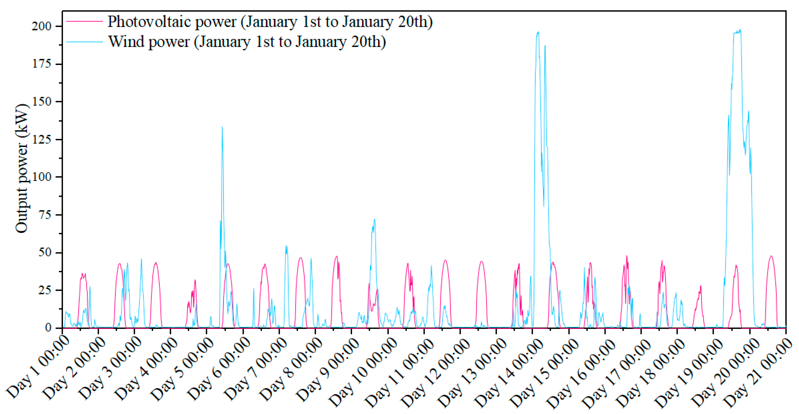
In this paper, the actual generation power data from photovoltaic and wind in northern China are selected for model training, as shown in

Table 2. Summary of the experimental dataset.

Category	Variable Name	Unit	Number of Data Points	Source
Power Generation	Photovoltaic Power	kW	1920	Actual monitoring records
	Wind Power	kW	1920	Actual monitoring records
Meteorological Data	Solar Radiation Intensity	W/m2	1920	Actual monitoring records
	Wind Speed	m/s	1920	Actual monitoring records
	Ambient Temperature	°C	1920	Actual monitoring records
	Wind Direction	° (degrees)	1920	Actual monitoring records
Temporal Resolution	Sampling Interval	/	15 min	/
Total Duration	/	/	20 days	/

. The data primarily encompasses wind direction, wind speed, solar radiation intensity, and other characteristic variables. Notably, the generation power data for both wind power and photovoltaic are shown in Figure 3. The skewness and peaks of photovoltaic within the same time period are relatively small and the data distribution is much uniform. Conversely, the data for wind power show a wider range of variation, indicating that wind power is more prone to fluctuations and has a higher likelihood of extreme values. This is primarily attributed to the fact that wind speed can fluctuate significantly over short periods, whereas solar radiation intensity remains more stable. The photovoltaic data during its output period after sunrise exhibits skewness and kurtosis values both close to zero, indicating a more uniform and symmetric distribution. In contrast, the wind power data demonstrates significantly higher skewness and kurtosis, suggesting a higher probability of extreme high values. This confirms that wind power exhibits larger variations and more intense fluctuations. These characteristics primarily stem from the rapid and substantial short-term variations in wind speed, while solar radiation intensity remains relatively stable. There is a significant difference in the degree of fluctuation between photovoltaic and wind power, and both exhibit strong stochasticity and nonlinearity, thereby increasing the complexity of prediction. Traditional prediction methods often suffer from low temporal resolution and prediction accuracy, making it challenging to accurately predict renewable energy generation.

Although the time span of the data is relatively short, this choice is primarily based on technical reasons and experimental considerations, aiming to verify the core performance of the proposed hybrid prediction model in short-term, high-volatility scenarios. In practical engineering applications, long-term, high-frequency wind and solar power generation data that include complete meteorological characteristics (such as wind speed and radiation intensity) are usually difficult to obtain. The 20-day dataset adopted in this study provides continuous, complete high-quality samples, which are sufficient to capture the typical fluctuation patterns of wind and solar power generation (e.g., daily cycles and sudden weather changes), thus offering effective support for verifying the model’s ability to handle non-stationarity and intermittency. The experimental design focuses on the horizontal comparison of performance differences between different prediction methods (time series, multivariate, and post-decomposition prediction) based on the same dataset. Verifying the superiority of the proposed method within a limited but representative data period, the conclusions of this study hold clear reference values for short-term prediction scenarios.

3.2. Data Decomposition

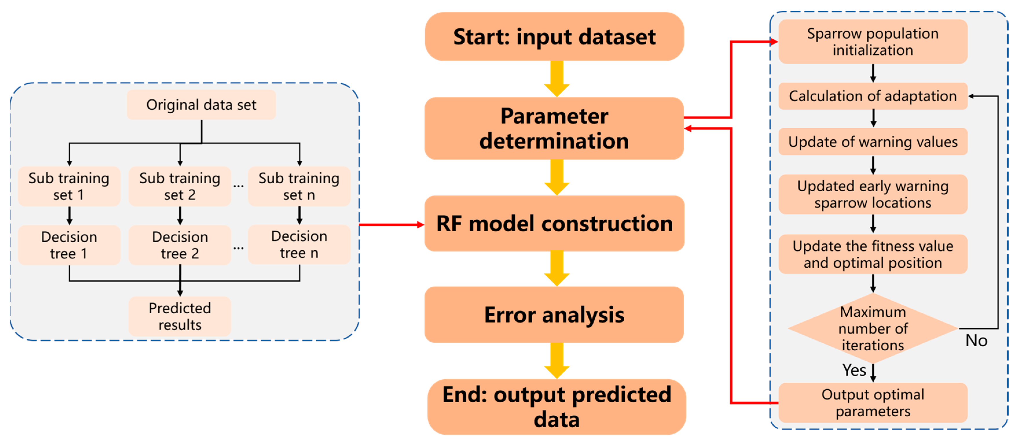
Before performing the VMD data decomposition, the SSA is used to optimize the minimum envelope entropy and determine the corresponding optimal modal component K and penalty factor α. The optimization intervals for the modal component K and the penalty factor α are set to [3, 10] and [100, 2500]. The main parameter settings of the SSA are as follows: the number of optimization variables is 2, the number of iterations is 15, and the population size is 10.

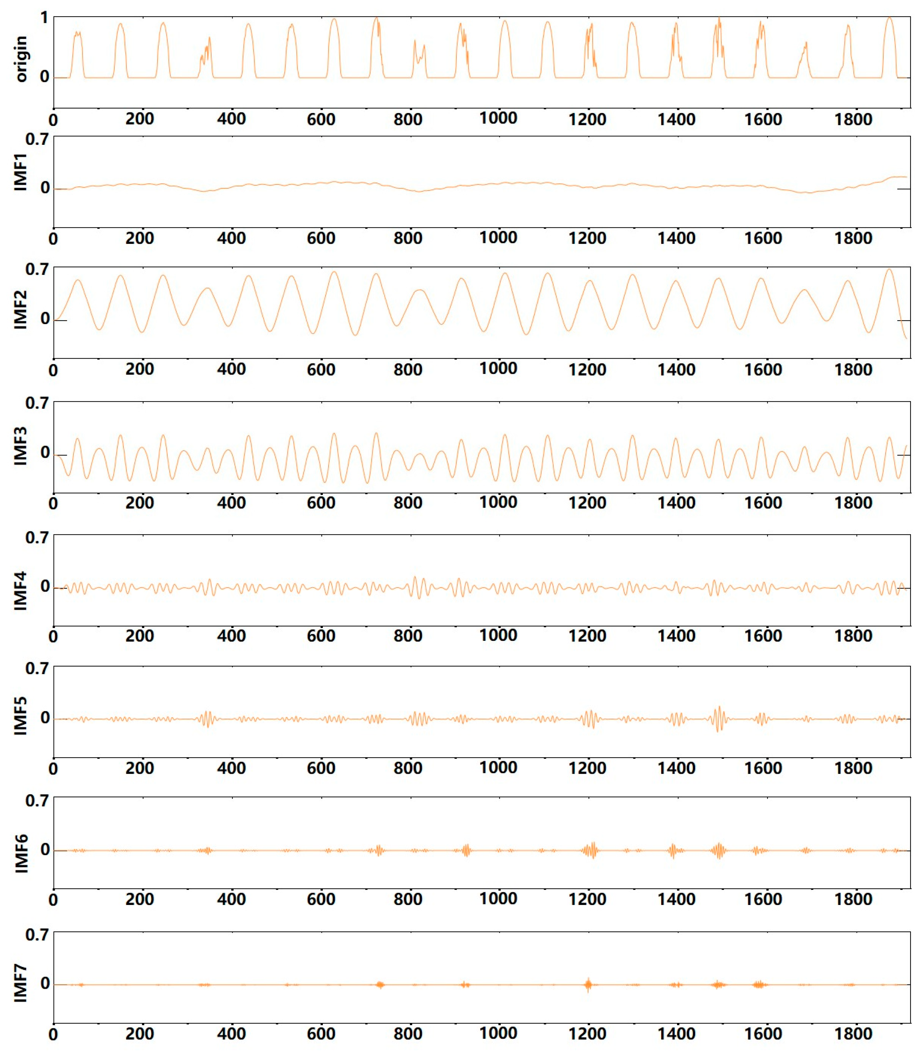
The optimization results show that the minimum envelope entropy of photovoltaic is 6.27, corresponding to an optimal modal component K of 7, and a penalty factor α of 302. This indicates that the data of photovoltaic is decomposed by VMD into seven decomposed signals. Similarly, the minimum envelope entropy of wind power is 6.67, corresponding to an optimal modal component K of 4 and a penalty factor α of 100. This means that the data of wind power is decomposed to obtain four decomposition signals. 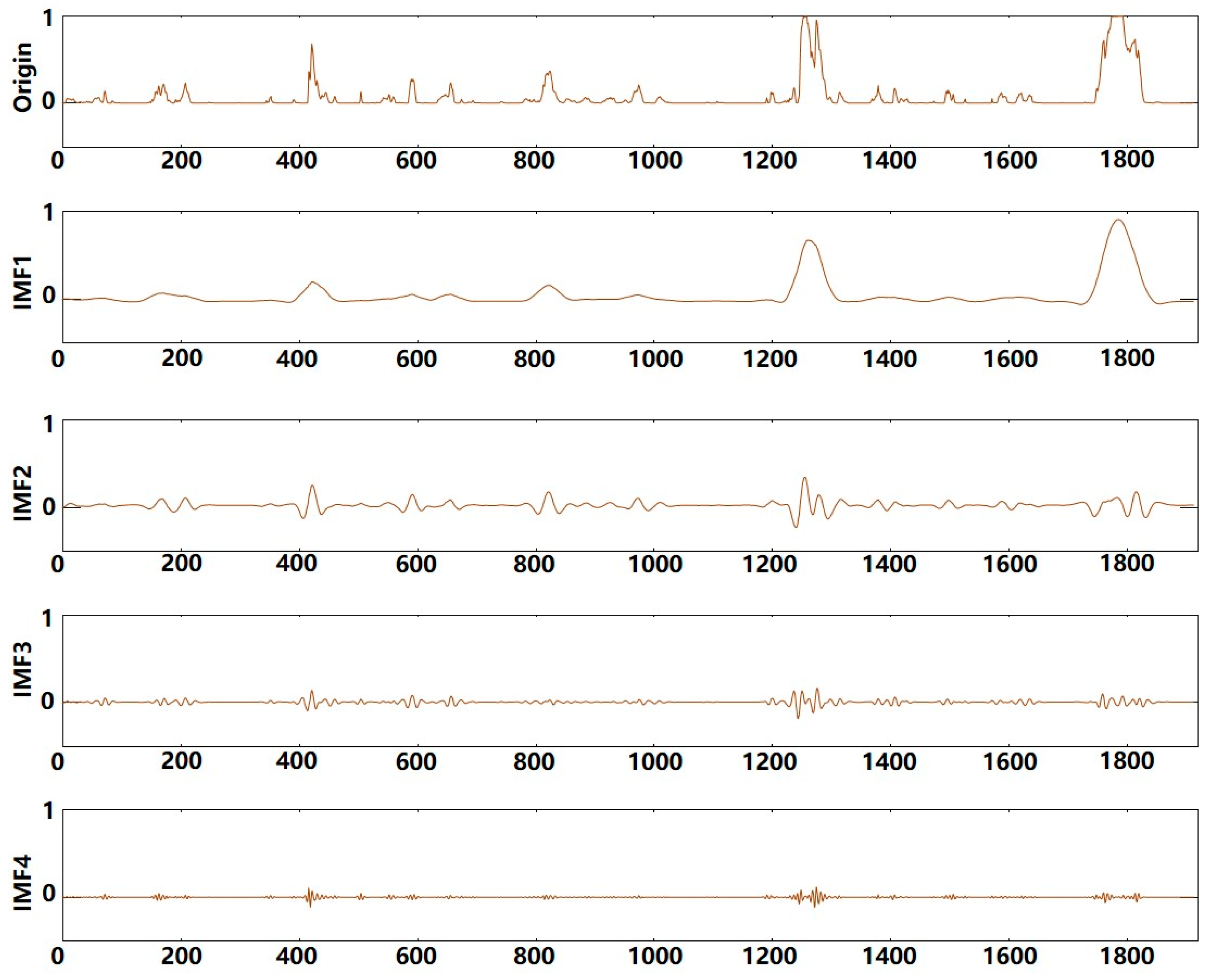Figure 4 and Figure 5 show the decomposition results. Notably, the prediction process excludes the residual sequences, as they are considered noise [23].

3.3. Pearson Correlation Analysis

The correlation test between raw data and IMFs using the PCC is presented in

Table 3. Photovoltaic power IMF correlation analysis results.

Name	IMF1	IMF2	IMF3	IMF4	IMF5	IMF6	IMF7
PCC	0.193	0.789	0.599	0.216	0.131	0.079	0.047

and

Table 4. Wind power IMF correlation analysis results.

Name	IMF1	IMF2	IMF3	IMF4
PCC	0.942	0.441	0.227	0.106

. The results of the PCC values for the photovoltaic power IMFs with respect to the raw data indicate that the most strongly correlated intrinsic modal function is IMF2, with a value of 0.789, signifying a strong correlation. Following this is IMF3, with a PCC value of 0.599, indicating moderate correlation. The least correlated intrinsic modal function is IMF7, with a value of 0.047, classified as low or no correlation.

In the case of wind power, the intrinsic modal function that exhibits the strongest correlation with the raw data is IMF1, with a PCC value of 0.942, which represents an extremely strong correlation. The least correlated intrinsic mode function is IMF4, with a value of 0.106, falling into the category of low or no correlation. Again, it is shown that IMF4 has the worst linear correlation with the original data and that changes in the original data have the least effect on IMF4.

In summary, due to the insufficient feature information extracted from the raw signals for photovoltaic power IMF7 and wind power IMF4, it is necessary to combine these IMFs with weather feature parameters for simultaneous prediction in order to enhance prediction accuracy. On the other hand, IMFs with high PCC values do not require the consideration of weather characteristic parameters.

3.4. Predictive Results and Error Analysis

In order to verify the superiority of the hybrid prediction method presented in this study for predicting photovoltaic and wind power generation, firstly, each IMF combined with weather characteristic parameters is predicted individually, while the remaining IMFs are predicted using a time series approach (abbreviation: IMF_wN). Then, all predictive results are integrated to derive the final predictive results. This allows for a comparison to determine which IMF, when combined with weather characteristic parameters, yields the most effective prediction performance. Secondly, the superiority of the proposed hybrid prediction method is further validated by contrasting its results with those of other methods, namely, time series prediction, multivariate prediction (considering weather characteristic parameters), and the combination of VMD with a prediction model. Finally, by substituting different benchmark models, comparative analysis is conducted to ascertain which benchmark model is most compatible with the hybrid prediction method proposed in this study.

3.4.1. Analysis of Prediction Results for SSA-RF

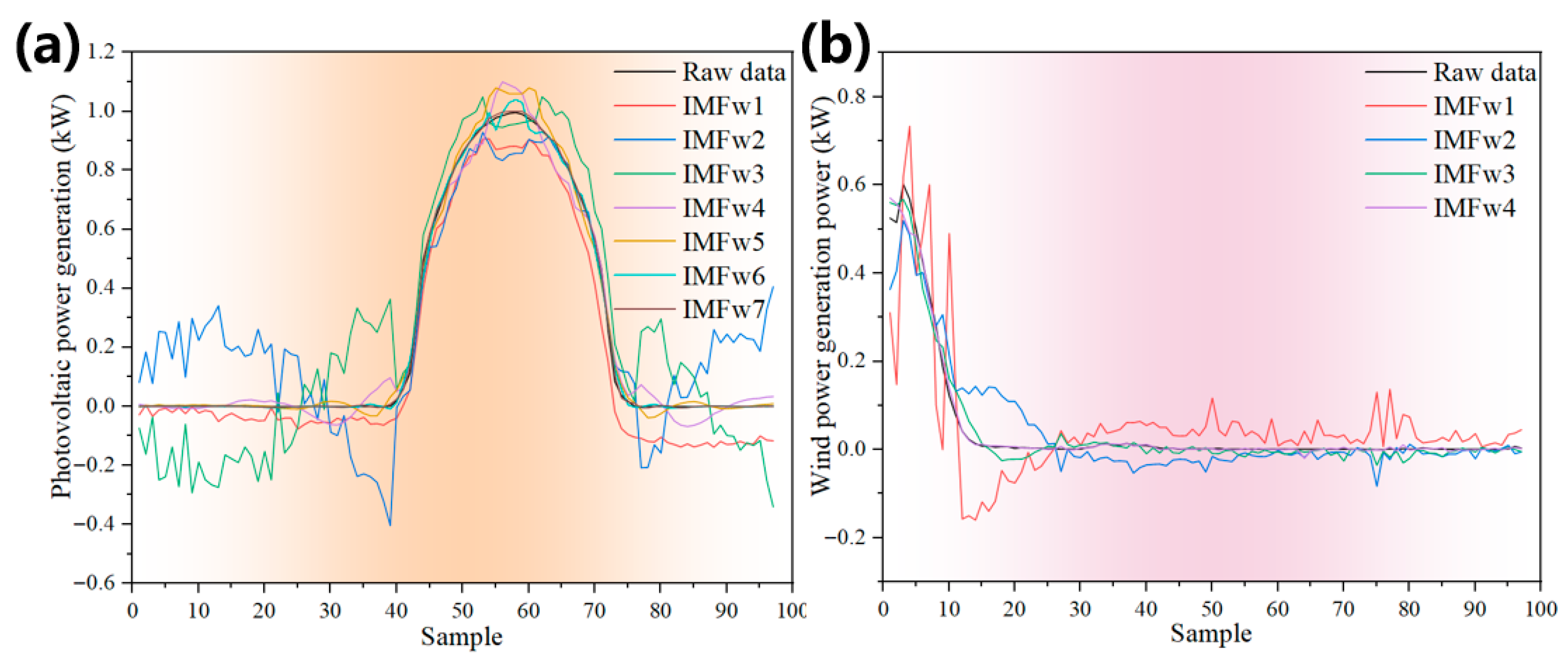
Figure 6a,b shows the prediction results for photovoltaic and wind power using the VMD-PCC-SSA-RF method. The prediction results for photovoltaic indicate that IMF_w7 exhibits the best performance among IMF_w1–IMF_w7, fitting outliers effectively. In contrast, the predicted values for IMF_w1–IMF_w6 show significant fluctuations at extreme points and varying degrees of hysteresis.

Table 5. Results of predicted performance evaluation indicators.

Category	Intrinsic Mode Function	MAE	RMSE	R2
Photovoltaic power	IMFw1	0.075	0.086	0.988
	IMFw2	0.137	0.169	0.812
	IMFw3	0.138	0.164	0.869
	IMFw4	0.033	0.043	0.987
	IMFw5	0.021	0.032	0.995
	IMFw6	0.009	0.016	0.998
	IMFw7	0.004	0.007	0.999
Wind power	IMFw1	0.06	0.091	0.627
	IMFw2	0.036	0.053	0.843
	IMFw3	0.014	0.02	0.979
	IMFw4	0.005	0.012	0.991

presents the prediction results for photovoltaic and wind power IMF_wN using the VMD-PCC-SSA-RF approach, revealing that IMF_w7 for photovoltaic has the lowest MAE and RMSE, along with the highest R², compared with IMF_w1–IMF_w6. Specifically, MAE is reduced by 55.56% to 97.1% and RMSE by 56.25% to 95.86%, and R² exceeds 0.999. For wind power generation, the predicted values of IMF_w4, when combined with weather characteristics, align more closely with the actual values than those of IMF_w1–IMF_w3. This results in a reduction in MAE by 64.29% to 91.67% and RMSE by 40% to 86.81%, and an R² closest to 1. Overall, the results demonstrate that the VMD-PCC-SSA-RF method yields the best prediction results for photovoltaic IMF_w7 and wind IMF_w4.

Combined with the analysis of the above results, it can be seen that the prediction performance enhances as the PCC value of the IMF decreases. This underscores the effectiveness of combining IMF with low PCC values and weather characteristic parameters in improving prediction accuracy. The rationale behind this is that a low PCC value for an IMF suggests a weak correlation with the original data, incomplete feature information extraction, necessitating the integration of additional features to enhance prediction accuracy. Conversely, IMF with high PCC values inherently possess more comprehensive feature information about the original data and may not require external predictors [39].

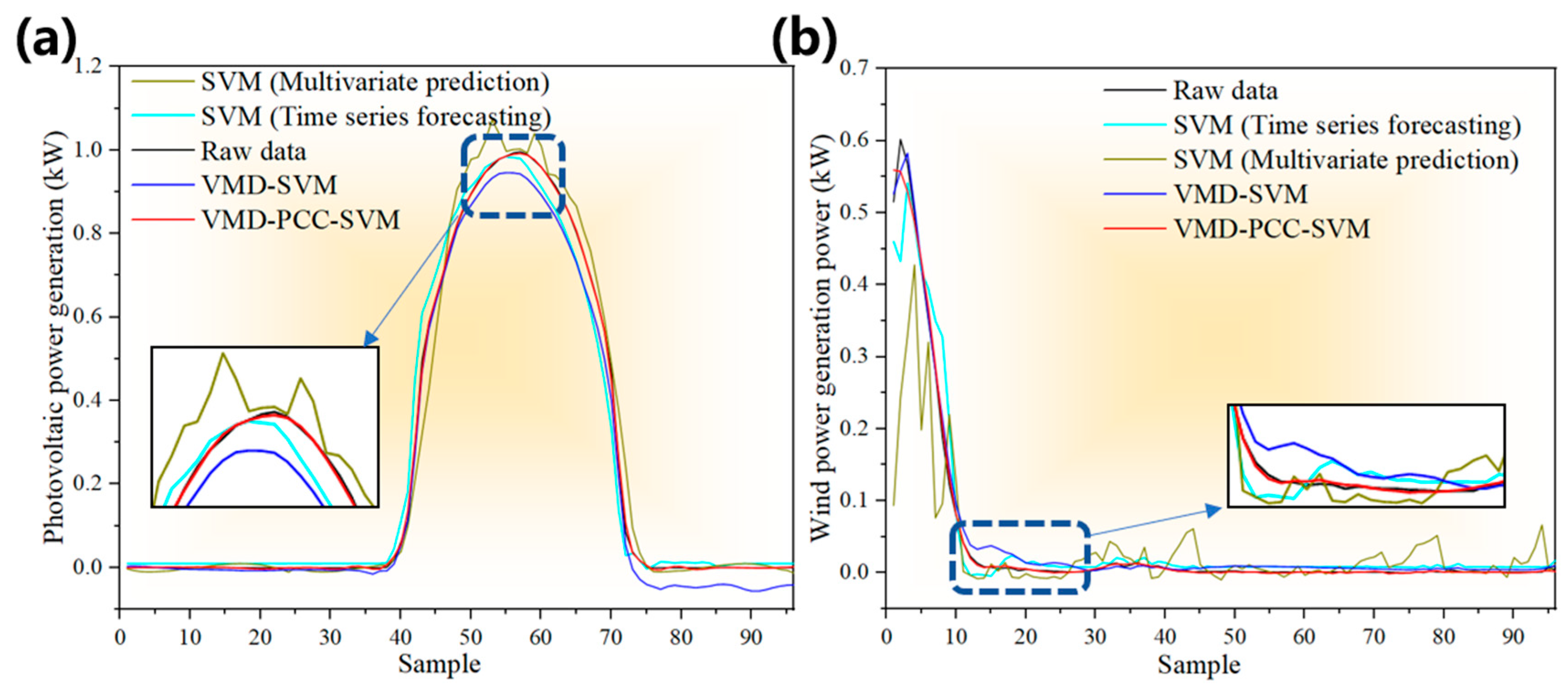
To better comprehend the accuracy of the prediction methods introduced in this study, this section focuses on predicting the generation power of photovoltaic and wind power using various methods: SSA-RF time series prediction, SSA-RF multivariate prediction (incorporating weather characteristic parameters), VMD-SSA-RF prediction, and the novel VMD-PCC-SSA-RF method proposed herein, as illustrated in Figure 7.

The prediction results for both photovoltaic and wind power generation are shown in Figure 7a,b. Notably, the VMD-PCC-SSA-RF method exhibits the most optimal fitting effect. Specifically, for photovoltaic, the prediction method presented in this study effectively mitigates the hysteresis issues encountered by other methods and demonstrates superior performance at extreme points when compared with other prediction curves. Similarly, for wind power, the VMD-PCC-SSA-RF method aligns more closely with the actual data than other methods, while the other methods exhibit varying degrees of lag. In summary, the prediction method proposed in this study has smaller prediction fluctuations, higher stability and higher reliability.

Table 6. Results of accuracy evaluation indicators for different prediction methods.

Category	Methods	MAE	RMSE	R2
Photovoltaic power	SSA-RF (Time series prediction)	0.022	0.021	0.982
	SSA-RF (Multivariate prediction)	0.03	0.065	0.975
	VMD-PCC-SSA-RF	0.004	0.007	0.999
	VMD-SSA-RF	0.045	0.062	0.984
Wind power	SSA-RF (Time series prediction)	0.012	0.038	0.948
	SSA-RF (Multivariate prediction)	0.029	0.079	0.655
	VMD-PCC-SSA-RF	0.005	0.012	0.991
	VMD-SSA-RF	0.012	0.025	0.974

presents the results of the accuracy evaluation metrics for various prediction methods. For photovoltaic, compared with SSA-RF (Time series prediction), SSA-RF (Multivariate prediction), and VMD-SSA-RF, the VMD-PCC-SSA-RF method reduces MAE by 81.74%, 86.67%, and 91.11%, respectively. Similarly, RMSE decreases by 66.67%, 89.23%, and 88.71%, respectively. However, the range of variation in R² is not significant. Turning to wind power, the VMD-PCC-SSA-RF method also outperforms others, compared with SSA-RF (Time series prediction), SSA-RF (Multivariate prediction), and VMD-SSA-RF, the VMD-PCC-SSA-RF method reduces the MAE by 58.33%, 82.76%, and 58.33%. The RMSE was reduced by 68.42%, 84.81%, and 52%, respectively. Notably, the results of the evaluation metrics proved that the hybrid prediction method proposed in this study can effectively improve the prediction accuracy.

3.4.2. Analysis of Prediction Results for BP Neural Network

This study proposes a prediction method grounded in the VMD-PCC model, utilizing SSA-RF as the benchmark model. To validate the reliability of the proposed prediction approach, this section employs the representative BP neural network of feed-forward neural networks to test the method and assess the prediction performance through error evaluation indices.

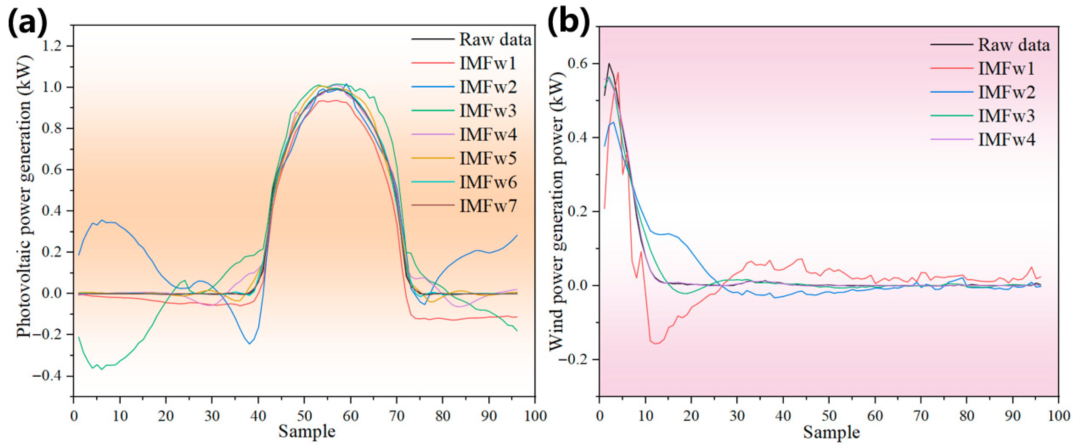
A comparison is made of the prediction results achieved by different IMFs in conjunction with weather feature parameters, as illustrated in Figure 8a,b. The results of the evaluation metrics are presented in

Table 7. Results of predicted performance evaluation indicators.

Category	Intrinsic Mode Function	MAE	RMSE	R2
Photovoltaic power	IMFw1	0.081	0.094	0.986
	IMFw2	0.123	0.153	0.857
	IMFw3	0.134	0.15	0.903
	IMFw4	0.036	0.046	0.956
	IMFw5	0.025	0.037	0.994
	IMFw6	0.006	0.011	0.999
	IMFw7	0.003	0.005	0.9998
Wind power	IMFw1	0.048	0.068	0.769
	IMFw2	0.034	0.05	0.837
	IMFw3	0.011	0.016	0.984
	IMFw4	0.003	0.008	0.996

. For photovoltaic power prediction, IMF_w7 exhibits superior predictive capabilities when compared with IMF_w1–IMF_w6, as evidenced by the evaluation index results. In particular, when compared with IMF_w1–IMF_w6, IMF_w7 reduces the MAE by 50–97.76%, decreases the RMSE by 54.55–96.73%, and achieves an R² closest to 1. For wind power prediction, IMF_w4 demonstrates strong predictive abilities, with the MAE reduced by 72.73–93.75%, the R decreased by 50–88.24%, and the R² improved by 1.22–29.52% when compared with IMF_w1–IMF_w3. The BP neural network predictions further confirm that the IMF with the lowest PCC value, when combined with weather feature parameters, can demonstrate excellent predictive abilities, aligning with the findings presented in Section 3.4.1.

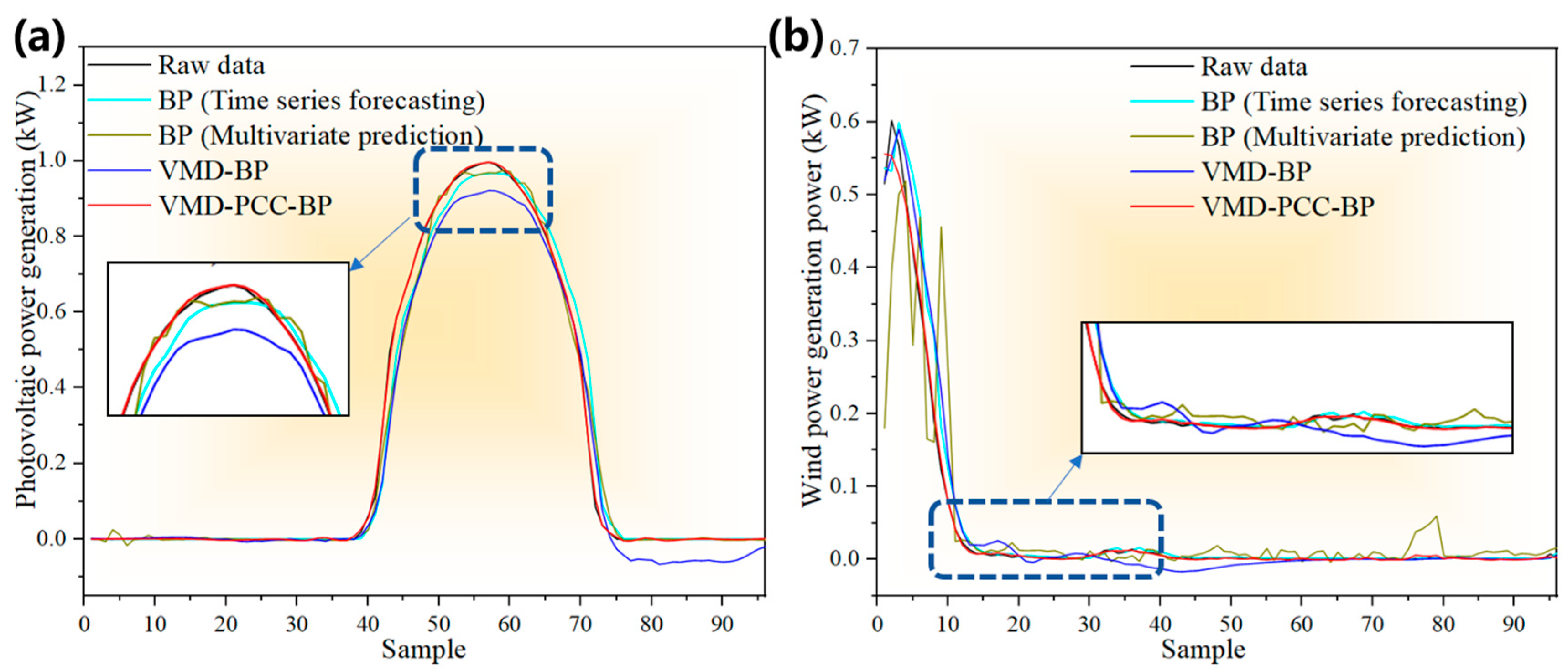
To further investigate whether the prediction accuracy of the methods proposed in this study is related to the benchmark model, the following research will employ BP time series prediction, BP multivariate prediction, VMD-BP prediction, and VMD-PCC-BP methods to predict the generation power of photovoltaic and wind power, as depicted in Figure 9a,b. Although the various methods exhibit distinct prediction effects during the prediction process, the VMD-PCC-BP curves demonstrate a closer fit to the raw data curves. This addresses the hysteresis issues present in other prediction methods, thereby underscoring the superiority of the prediction methods introduced in this study.

Table 8. Results of accuracy evaluation indicators for different prediction methods.

Category	Methods	MAE	RMSE	R2
Photovoltaic power	BP (Time series prediction)	0.021	0.045	0.986
	BP (Multivariate prediction)	0.019	0.04	0.989
	VMD-PCC-BP	0.003	0.005	0.999
	VMD-BP	0.036	0.052	0.988
Wind power	BP (Time series prediction)	0.009	0.026	0.975
	BP (Multivariate prediction)	0.023	0.061	0.757
	VMD-PCC-BP	0.003	0.008	0.996
	VMD-BP	0.013	0.026	0.97

presents the error evaluation results. For photovoltaic, the MAE of VMD-PCC-BP decreases by 84.21% to 91.67%, while the RMSE decreases by 87.5% to 90.38%. The overall R² remains relatively stable. For wind power, the MAE of VMD-PCC-BP decreases by 66.67% to 86.96%, the RMSE decreases by 69.23% to 86.89%, and the R² improves by 2.15% to 31.57%. These results underscore the high prediction accuracy of the method proposed in this study.

3.4.3. Analysis of Prediction Results for SVM

In this section, SVM is employed as a benchmark model to validate the prediction method introduced in this paper. The results of predicting each IMF of photovoltaic and wind power generation, combined with weather parameters, and summed with the time series prediction of their remaining IMF, are presented in Figure 10a and Figure 10b, respectively. These results are further analyzed in conjunction with

Table 9. Results of predicted performance evaluation indicators.

Category	Intrinsic Mode Functions	MAE	RMSE	R2
Photovoltaic power	IMFw1	0.067	0.077	0.99
	IMFw2	0.123	0.163	0.854
	IMFw3	0.116	0.151	0.909
	IMFw4	0.023	0.033	0.992
	IMFw5	0.016	0.021	0.997
	IMFw6	0.006	0.012	0.999
	IMFw7	0.003	0.005	0.9998
Wind power	IMFw1	0.048	0.071	0.68
	IMFw2	0.034	0.053	0.817
	IMFw3	0.009	0.016	0.984
	IMFw4	0.003	0.008	0.996

. Notably, photovoltaic IMF7 and Wind IMF4 exhibit the highest R² and the lowest MAE and RMSE, which align with the findings from the previous two sections. The IMF with the lowest PCC demonstrates the best prediction performance when combined with weather parameters.

Subsequently, the prediction efficacy of various prediction methods is compared. As illustrated in Figure 11a,b and analyzed alongside in

Table 10. Results of accuracy evaluation indicators for different prediction methods.

Category	Methods	MAE	RMSE	R2
Photovoltaic power	SVM (Time series prediction)	0.294	0.466	0.988
	SVM (Multivariate prediction)	0.025	0.044	0.989
	VMD-PCC- SVM	0.003	0.005	0.9998
	VMD- SVM	0.028	0.037	0.997
Wind power	SVM (Time series prediction)	0.013	0.028	0.953
	SVM (Multivariate prediction)	0.031	0.073	0.724
	VMD-PCC- SVM	0.003	0.008	0.996
	VMD- SVM	0.008	0.011	0.995

, VMD-PCC-SVM effectively addresses the hysteresis issue inherent in other prediction methods, achieving the highest R² and the lowest MAE and RMSE. This comprehensively validates the exceptional prediction performance of VMD-PCC-SVM.

3.4.4. Comparison of Prediction Results of Different Benchmark Models

Currently, the prevalent renewable energy prediction models include RFs, BP neural networks, and SVMs. In this section, the prediction performance of these three models is compared to determine the most suitable benchmark model when combined with VMD-PCC, as shown in

Table 11. Results of evaluation indicators for different benchmark models.

	Evaluation Indicators	SSA-RF	BP Neural Network	SVM
Photovoltaic power	R2	0.999	0.9998	0.9998
	RMSE	0.007	0.0055	0.0053
	MAE	0.004	0.0031	0.0029
Wind power	R2	0.991	0.9958	0.9957
	RMSE	0.012	0.0082	0.0082
	MAE	0.005	0.0031	0.0031

. Upon observation, it is evident that the evaluation indices of the prediction results for the three benchmark models are relatively close, which underscores the versatility of the VMD-PCC prediction method.

For photovoltaic prediction, the benchmark model with the optimal prediction performance is SVM, exhibiting the R² closest to 1 and the smallest MAE and RMSE, both of which are lower than those of SSA-RF. Similarly, for wind power prediction, SVM remains the benchmark model with the best prediction performance, with MAE and RMSE comparable to those of BP neural network but with an R² closest to 1. Therefore, the most appropriate benchmark model for VMD-PCC, the research method proposed in this paper, is SVM.

In summary, the hybrid prediction method proposed in this study has excellent prediction performance in predicting renewable energy generation, and the prediction performance does not change significantly after replacing the benchmark model, which proves the universality of the hybrid prediction method. In order to better improve the prediction performance of the hybrid prediction method, the benchmark model that is more suitable for the hybrid prediction method is SVM, as shown by the results in this section. Compared with current studies, for instance, the studies in References [23,33] also used VMD but did not perform IMF selection. In contrast, the method in this study selects key IMFs via the PCC, which has achieved better results in terms of reducing lag.

3.5. Analysis of Room Temperature Fluctuations

Accurate prediction results can effectively enhance the economic efficiency and operational reliability of energy supply systems, which is mainly reflected in optimizing energy scheduling, reducing energy consumption, and proactively addressing load fluctuations to mitigate equipment overload. According to the research findings, the most suitable benchmark model for VMD-PCC is identified as SVM. Therefore, this section applies the VMD-PCC-SVM model and other different research methods (SVM-single variable prediction, SVM-multivariate prediction, and VMD-SVM) to the heating system. Prediction errors directly cause issues such as insufficient or excessive heating in the system, leading to fluctuations in room temperature.

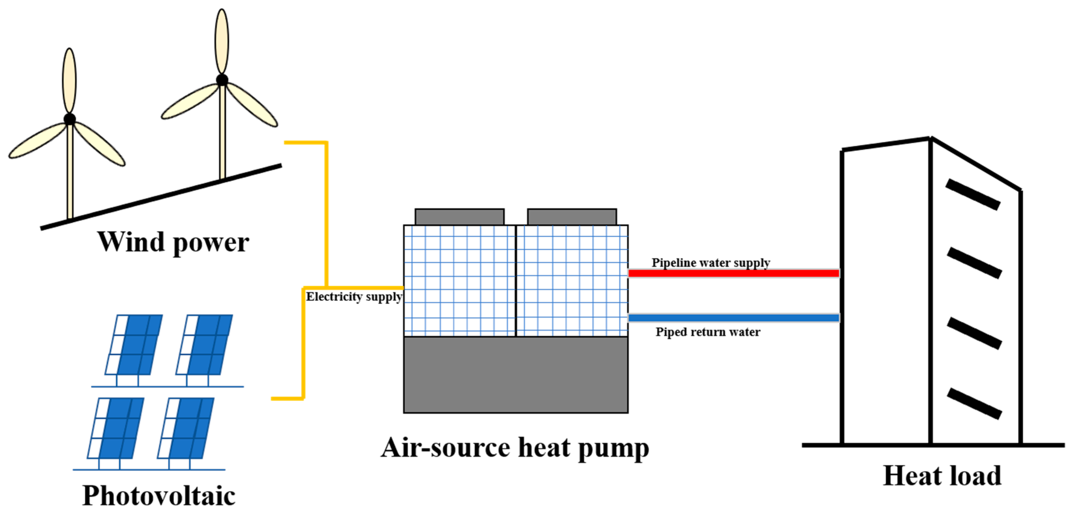
In this study, a room with dimensions of 1 m (length) × 1 m (width) × 2 m (height) is selected as the research object, where the heating is provided by embedded pipelines in the interior walls for heat dissipation. Based on cluster analysis, a typical winter day was selected as a case study for the research. Photovoltaic and wind power serve as the primary energy inputs to supply electricity to an air-source heat pump, which acts as the heating equipment. The air-source heat pump supplies hot water to the user side via pipelines, as illustrated in Figure 12. The heating system is designed to supply heat 24 h a day. The indoor temperature corresponding to the original data used in the prediction model is set as the baseline scenario, while the prediction results of different models serve as control groups. The operation status of the heating system is adjusted based on prediction errors, and the indoor temperatures of the baseline scenario are compared with those of other prediction models.

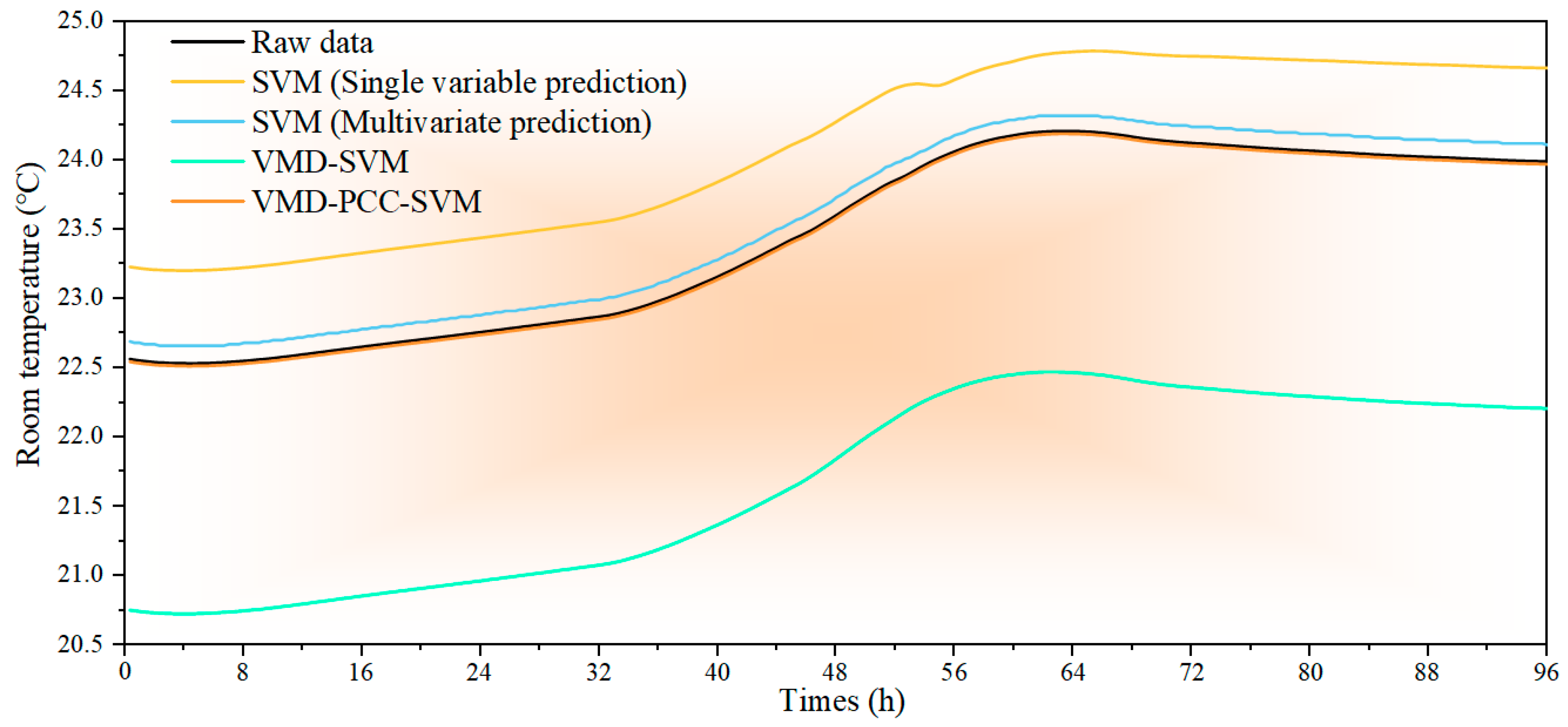
Figure 13 shows the indoor temperature changes corresponding to different prediction methods, and

Table 12. Quantitative results.

	Raw Data	SVM-Single Variable Prediction	SVM-Multivariate Prediction	VMD-SVM	VMD-PCC-SVM
MAE	0	0.652	0.124	1.775	0.019
RMSE	0	0.654	0.124	1.776	0.019

presents the quantitative results of indoor temperature variations. Compared with the original data, VMD-SVM exhibits the largest room temperature fluctuations, with MAE and RMSE values of 1.775 and 1.776, respectively. Followed by SVM-single variable prediction, where MAE and RMSE decrease by 63.27% and 63.18%, respectively, compared with VMD-SVM. Next is SVM-multivariate prediction, with MAE and RMSE decreasing by 93.01% and 93.02%, respectively, relative to VMD-SVM. VMD-PCC-SVM shows the smallest room temperature fluctuations, with the lowest MAE and RMSE values. Compared with other prediction methods, it has the highest consistency with the original data, enabling the heating system to adjust according to demand, avoid excessive or insufficient heating, and effectively reduce energy consumption.

In terms of energy consumption, taking the entire heating season as an example, the power consumption of the heating system corresponding to the original data is 76.58 kWh. SVM-single variable prediction has the highest power consumption at 80.08 kWh, followed by SVM-multivariate prediction at 77.68 kWh. VMD-SVM reduces the power consumption to 73.71 kWh, while VMD-PCC-SVM consumes 76.47 kWh, which is closest to the original data’s power consumption. Analyzing in combination with room temperature fluctuations, although VMD-SVM has the lowest energy consumption, its significant room temperature fluctuations fully demonstrate large prediction errors, leading to unstable operation of the heating system. While energy consumption is reduced, room temperature comfort is compromised. SVM-single variable prediction has the highest energy consumption, where prediction errors may cause frequent operational adjustments or excessive heating in the system, leading to energy waste and equipment damage. VMD-PCC-SVM’s energy consumption is very close to the original data, with the smallest room temperature fluctuations, indicating that the proposed prediction method in this study has excellent predictive performance. It maintains a stable room temperature and avoids unnecessary energy consumption, achieving a good balance between energy consumption and heating stability. SVM-multivariate prediction has slightly higher energy consumption than the original data and relatively smaller temperature fluctuations, but its stability is not as good as VMD-PCC-SVM.

These research results indicate that accurate prediction results directly impact the energy consumption of heating systems and room temperature control effects. The prediction results of VMD-PCC-SVM have small errors and are very close to the actual power generation, achieving dual advantages of reasonable energy consumption and stable room temperature. This provides an important basis for selecting prediction methods in practical heating systems and fully demonstrates the critical role of precise prediction in improving energy utilization efficiency and heating comfort.

4. Conclusions

This study has presented a hybrid prediction method that integrated VMD and PCC to address the inherent characteristics of photovoltaic and wind power generation, notably volatility and discontinuity. The proposed method initially tackled complex data by adopting envelope entropy as the fitness function and utilizing SSA to optimize VMD’s parameters, thereby enhancing data decomposition performance. Subsequently, the PCC was employed to conduct a correlation analysis between the IMFs and the original data, facilitating the filtering of the least relevant IMFs. These least relevant IMFs, in conjunction with weather feature parameters, make predictions, which then add up the predict derived from the remaining IMFs to yield the final prediction results. To substantiate the prediction performance of this method, actual photovoltaic and wind power generation data were utilized for verification. The conclusions drawn from this verification are as follows:

(1)

In comparison with other prediction methods, this prediction method demonstrates superior performance for photovoltaic and wind power generation prediction, effectively mitigating the issue of prediction lag and exhibiting greater stability. R² can be as high as 0.999 or more.

(2)

By incorporating the IMF with the lowest PCC value relative to the original data, along with weather feature parameters, into the prediction process, a notable improvement in prediction accuracy is achieved. Furthermore, this approach remains accurate even in the presence of abnormal data.

(3)

This prediction method excels at predicting both photovoltaic and wind power generation with remarkable accuracy. Notably, altering the benchmark model does not significantly impact the prediction accuracy, the R² was all greater than 0.99, the RMSE was all in the range of 0.0053–0.012, and the MAE was all in the range of 0.0029–0.005, underscoring the stability and effectiveness of this prediction method, as evidenced by the experiments conducted.

(4)

In heating systems, accurate prediction models play a crucial role in regulating indoor temperature on the load side. Experimental results show that the prediction method proposed in this study exhibits the best performance in terms of energy consumption and room temperature stability, with its energy consumption close to the original data and minimal room temperature fluctuations. Thus, it is evident that precise predictive performance is essential for balancing energy consumption and comfort in heating systems.

This study still has certain limitations: First, model training and validation are based on short-term data (20 days), and its long-term generalization ability—especially its adaptability to different seasonal patterns—needs to be further verified. Second, the current research is focused on a simulation environment and has not yet undergone engineering tests in large-scale actual building energy systems. Although the hybrid forecasting method proposed in this study demonstrates excellent performance in wind and solar power prediction, there remain areas worthy of further exploration and refinement, including validation of reliability, research on prediction uncertainty quantification, and expansion of prediction targets and application domains.