Article

Does the Multi-Scale Built Environment Impact on Residents’ Subjective Well-Being?

1
Architecture and Civil Engineering Institute, Guangdong University of Petrochemical Technology, Maoming 525000, China
2
Faculty of Innovation and Design, City University of Macau, Macau 999078, China
3
Faculty of Fine and Applied Art, Suan Sunandha Rajabhat University, Bangkok 10700, Thailand
*
Authors to whom correspondence should be addressed.
These authors contributed equally to this work.
Buildings 2025, 15(18), 3311; https://doi.org/10.3390/buildings15183311
Submission received: 29 July 2025 / Revised: 5 September 2025 / Accepted: 10 September 2025 / Published: 12 September 2025

Abstract

Previous studies have demonstrated that the built environment has a significant impact on individual subjective well-being (SWB). However, the majority of these studies primarily examined the impacts of community-level environments on subjective well-being, with limited exploration of the influence of multi-scale environments. This study addresses this gap by utilizing questionnaire surveys and built environment data to examine the effects of built environments at the housing, neighborhood, and community scales on subjective well-being through a multiple regression model (specifically, a hierarchical regression). The results show that environmental variables at the housing scale, neighborhood scale, and community scale can significantly improve the explanatory power of life satisfaction (LS). The findings reveal that the explanatory power of environmental variables on life satisfaction exhibits a diminishing trend from proximate to distal scales. It was found that, in terms of the housing scale, the housing construction environment and quality and the increase in per capita housing area positively contribute to residents’ life satisfaction. At the neighborhood scale, a comfortable environment and enhanced facilities are conducive to improving residents’ life satisfaction, whereas the evaluation of property management and services is linked to reduced life satisfaction. At the community scale, the increase in building density (BD), functional mix density (FMD), road intersection density (RID), and bus stop density (BSD) is not conducive to enhancing residents’ life satisfaction. However, higher bus line density (BLD) is positively correlated with the improvement of residents’ life satisfaction. These findings suggest that in urban community planning and management, attention should be paid not only to housing-scale environmental elements but also to neighborhood-scale environmental elements, and they emphasize the rational planning of community scale environments to enhance residents’ subjective well-being.

1. Introduction

The pursuit of sustainable and healthy cities has become a central goal of global development, with enhancing residents’ subjective well-being (SWB) recognized as a key objective [1]. As an important dimension of subjective well-being (SWB), life satisfaction refers to people’s overall cognitive evaluation of life [2]. A high level of life satisfaction contributes to enhancing SWB, maintaining health, and extending lifespan [3]. However, China’s long-term strategy of prioritizing development has led to economic prosperity and improved living conditions, but also resulted in a range of urban challenges [4]. Although urbanization has historically aimed to improve living standards, it has not consistently enhanced residents’ happiness and may even reduce it in some contexts [5]. Continuously enhancing residents’ subjective well-being has become an important task for China’s high-quality development, and the construction of healthy and happy cities [6]. Therefore, identifying how environmental quality can be improved to enhance life satisfaction is a critical issue in geographical and urban planning research [1,7].
Research on subjective well-being involves multiple disciplines with different focuses, and related research in geography and urban planning disciplines started relatively late [6,8]. Existing studies have established that the built environment significantly influences individual SWB [9], with specific features at the housing, neighborhood, and community levels playing crucial roles [10,11]. Methodologically, researchers commonly employ correlation analysis, regression models, and ordered response models to examine these relationships [12,13,14,15]. However, much of this work remains siloed within single spatial scales, examining either macro-level community factors or micro-level housing attributes, without integrating multiple scales [1,6,7,13,16]. Only a limited number of studies adopt a multi-scale or multi-dimensional perspective [6,17,18,19], and even fewer simultaneously incorporate both objective and subjective measures of the built environment [8,20]. This is a significant limitation, as relying solely on one type of data may lead to biased or incomplete conclusions [8,20].
Given these gaps, this study aims to provide a more integrated examination of how built environments at multiple scales—housing, neighborhood, and community—affect life satisfaction, using both subjective perceptions and objective spatial data. Specifically, we address the following research question: Do environmental factors at different scales (housing, neighborhood, and community) significantly enhance the predictive power of life satisfaction models? By doing so, this research contributes to the literature by offering a holistic understanding of the multi-scale mechanisms influencing SWB, thereby providing an empirical basis for targeted urban planning and policy interventions aimed at enhancing residents’ quality of life.

2. Literature Review and Model Development

2.1. Subjective Well-Being

Subjective well-being (SWB), a central concept in positive psychology and social sciences, refers to individuals’ multifaceted evaluations of their lives and emotional experiences. These evaluations encompass both cognitive judgments of life satisfaction and affective experiences related to emotions and moods [1]. SWB is characterized by its subjective nature, relying on personal criteria rather than objective conditions, and its relative stability over time [3,21]. The study of SWB typically distinguishes between two primary philosophical traditions and their corresponding components: the hedonic perspective and the eudaimonic perspective [22]. The hedonic tradition, often synonymous with SWB itself, focuses on the pursuit of pleasure and avoidance of pain. It is operationally defined as comprising three distinct yet related components: (1) Life satisfaction (LS)—The cognitive component, involving a global judgment of one’s life as a whole according to self-selected standards [23]. (2) Positive affect (PA)—The experience of frequent pleasant emotions such as joy, contentment, and happiness. (3) Negative affect (NA)—The experience of infrequent unpleasant emotions such as sadness, anger, and anxiety. The eudaimonic tradition, in contrast, emphasizes living in accordance with one’s true self (daimon), and focuses on meaning, self-realization, and the fulfillment of human potential [24]. While related, eudaimonic well-being (often measured through concepts like psychological well-being) is considered a distinct construct.
Given its cognitive, evaluative, and relatively stable nature, life satisfaction is particularly relevant for studies investigating the long-term impact of contextual factors, such as the built environment [7]. Individuals can deliberately assess how their living conditions align with their aspirations, making LS a crucial indicator for urban planning and policy interventions aimed at improving the quality of life. Consequently, this study focuses specifically on the life satisfaction dimension of SWB, acknowledging its sensitivity to the external environmental factors under investigation. Moreover, a comprehensive understanding of SWB necessitates an examination of its myriad influencing factors, which range from internal personality traits to external socioeconomic and environmental conditions. These factors will be reviewed in detail in a latter section.

2.2. Built Environment

In the field of urban planning, in recent years, domestic and international empirical research results on the impact of built environments on subjective well-being have been gradually enriched. Numerous studies have established a strong correlation between life satisfaction and the built environment. The housing environment mostly comprises the housing building and its indoor environment. The neighborhood built environment refers to the built environment of closed or semi-closed neighborhood areas [11,25,26,27]. The neighborhood environment is closely related to the community environment and living environment in connection, and is mostly centered on residents, examining the overall situation of related infrastructure, service facilities, and psychological feelings [11].
The built environment typically encompasses various physical elements, such as land use, transportation systems, infrastructure, and spatial components [28]. Cervero and Kockelman initially proposed the “3D” model, emphasizing density, diversity, and design [29]. Subsequently, Ewing and Cervero expanded this model by incorporating Destination Accessibility and Distance to Transit, resulting in the widely acknowledged “5D” model [30]. However, both believe that the 5D model is still not rigorous enough, but that there is no better alternative model [31]. Therefore, this study also adopts the “5D” model as its framework. Moreover, regarding the complexity of the built environment, to fully understand its impact on humans, it is necessary to adopt community, multi-level, and interdisciplinary research methods [31,32].

2.3. The Factors Influencing Subjective Well-Being

A detailed review of the literature shows that research on factors affecting subjective well-being is mainly distributed in traditional disciplines such as economics and psychology, as well as emerging disciplines such as public health, geography, and urban planning [33]. Studies have shown that numerous factors affect subjective well-being, including demographic characteristics such as age and gender [34,35], socio-economic characteristics such as income, employment, and education [36], and family characteristics such as marital status [37]. In addition, optimists are better able to adapt to changes in life and show higher happiness [38]. Optimism is considered an important factor in predicting post-migration life satisfaction [39].
On the relationship between living environment and satisfaction, Campbell et al. proposed a theoretical model to illustrate the mechanism of community satisfaction [40]. The model proposes that attributes and evaluations at different scales, such as community, neighborhood, and housing, are closely related to satisfaction in related fields. Sirgy et al. linked neighborhoods, housing, families, communities, and life satisfaction, forming a framework for the impact of neighborhood characteristics on life satisfaction [41]. In summary, both models provide theoretical support for the study of multi-scale environments and life satisfaction. In terms of the built environment, in the specific context of China, in addition to the community built environment, housing and neighborhood areas, as the most important living and behavioral spaces for people, have a significant impact on residents’ life satisfaction [11,42]. It is worth noting that due to individual attribute differences, residents may have different perceptions and evaluations of the same community, neighborhood, and housing environment attributes, which may lead to differentiated impacts [43]. Therefore, considering both objective and subjective built environments in the study may be more conducive to research.
In terms of housing environment, studies have confirmed that housing newness, area size, age, housing natural environment (e.g., ventilation, lighting), and housing quality are related to subjective well-being [42,44,45]. In terms of neighborhood environment, studies have demonstrated that the green landscape, facilities, and comfort of neighborhood areas impact residents’ sense of place and life satisfaction [11]. Furthermore, exposure to the built environment and external surroundings plays a role in individuals’ well-being, with air quality and noise identified as notable factors affecting life satisfaction in some research [1].
In terms of community built environment, several studies have proven that higher urban density is beneficial to the environment [43] and helps enhance residents’ SWB. However, higher population density can reduce residents’ SWB [7,45,46,47]. Studies have shown that factors such as land use mix, diverse food acquisition methods, and various entertainment facilities have been shown to positively influence residents’ SWB [48], although they may also have adverse effects [7]. Additionally, reductions in road traffic dead ends can increase residents’ life satisfaction, while the increase in road connectivity may also reduce life satisfaction [7]. The accessibility of stores, educational facilities, public service facilities, and green parks is positively correlated with residents’ life satisfaction [1]. Furthermore, the availability of public transit stations and rail facilities can significantly improve public transport accessibility, thereby enhancing residents’ life satisfaction [49,50,51,52]. Lastly, improved destination accessibility has been found to positively impact subjective well-being [52,53,54].
Limited research has investigated the impact of multi-scale environments on well-being. Previous studies have indicated a significant correlation between residents’ SWB and the built environments of urban areas with over 50% urbanization [18]. Both housing and community environments significantly impact residents’ subjective well-being [11,42]. A study in China has demonstrated that various built environments at different scales, including neighborhoods, communities, and cities, collectively influence the leisure activities of the elderly [17]. Despite these findings, there remains a scarcity of studies examining the role of multi-scale, multi-dimensional environmental factors in subjective well-being [6]. Building upon the gaps and insights from existing literature, this study aims to further explore the impact of multi-scale built environments on life satisfaction.

2.4. Model Hypotheses

Based on the literature review and related theoretical analyses, this study attempts to examine the relationship between life satisfaction and the multi-scale built environment, namely, the housing scale, the neighborhood scale, and the community scale. The study uses data from social surveys conducted in China from 2021 to 2022 and built environment data obtained by geocoding, and employs a hierarchical regression model to examine the impact of multi-scale environments on life satisfaction (LS) (Figure 1). This study focuses on addressing the following three hypotheses:
Hypothesis 1.
The built environment at the housing scale can significantly improve the explanatory power of LS.
Hypothesis 2.
The built environment at the neighborhood scale can significantly improve the explanatory power of LS.
Hypothesis 3.
The built environment at the community scale can significantly improve the explanatory power of LS.

3. Methodology

3.1. Data Collection

Before data collection, the questionnaire was designed. The questionnaire primarily consists of three parts: a cover letter with consent form, the main questionnaire, and an acknowledgments section. The main questionnaire includes the following sections: Part 1 focuses on basic living conditions and housing evaluation; Part 2 assesses the perception and evaluation of the neighborhood; Part 3 evaluates life satisfaction, measuring residents’ living conditions, ideals, achievements, etc.; Part 4 is the Life Orientation Test—Revised (LOT-R) for measuring optimistic personality traits; and Part 5 collects personal socio-economic attributes. The questionnaire was refined through a pilot test and subsequent revisions before the formal survey was conducted.
The survey process was divided into three parts and administered on-site in both electronic and paper formats. First, before the survey began, respondents were asked to read the cover letter and sign the Informed Consent Form. Second, during the survey process, respondents with normal abilities independently completed the questionnaire, with researchers present to address any questions; for respondents with visual impairments or other vulnerabilities, researchers read the questions aloud and recorded oral responses. When respondents had questions or did not understand an item, survey personnel provided further explanations. The entire survey process took approximately 30–45 min to complete. Third, after the survey, questionnaires were collected, and respondents were thanked for their participation.
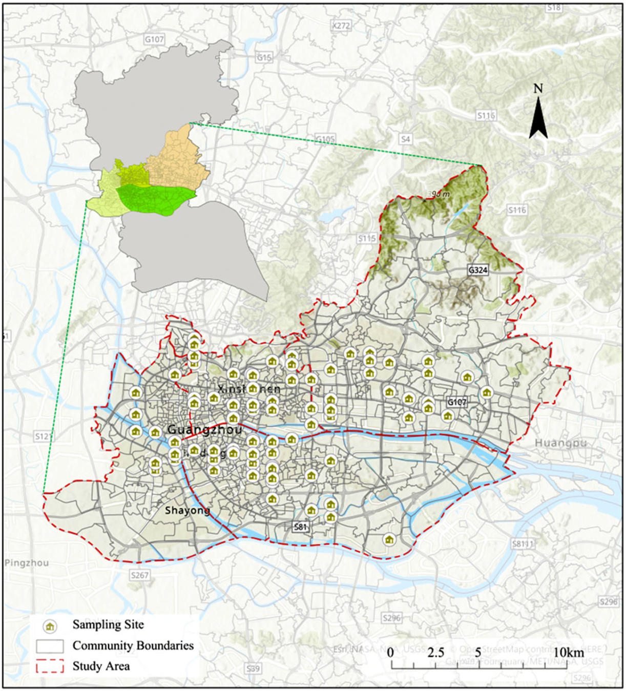
The central urban area of Guangzhou was selected as the study area due to its representativeness and relevance for examining the relationship between multi-scale built environments and subjective well-being. As a premier first-tier city and a key economic hub, Guangzhou embodies the rapid urbanization, high density, and complex urban fabric typical of major Chinese metropolises. It also exhibits pronounced socio-spatial diversity, encompassing varied residential forms—from urban villages and traditional neighborhoods to modern high-rise estates and new towns—enabling a robust analysis of built environment effects across scales. To empirically investigate this relationship, a sampling survey was conducted by the research team in the central urban area of Guangzhou City from June 2021 to August 2022, yielding sample data (Figure 2) focused on residents aged 18 and above residing in the city. A multi-stage stratified sampling and probability sampling method were used in the survey. Before sampling, the administrative districts were stratified according to the administrative areas to refine the sampling frame and improve representativeness. The administrative districts, streets, and neighborhood committees were sorted according to the permanent population size, and then randomly and equally selected administrative districts, streets, and neighborhood committees. Finally, within the selected neighborhood committees, random probability sampling of neighborhood areas was conducted, and households were surveyed according to the population ratio. A total of 621 questionnaires were collected, with 568 valid questionnaires, resulting in an efficiency rate of approximately 91.47%.

3.2. Variables and Measurement

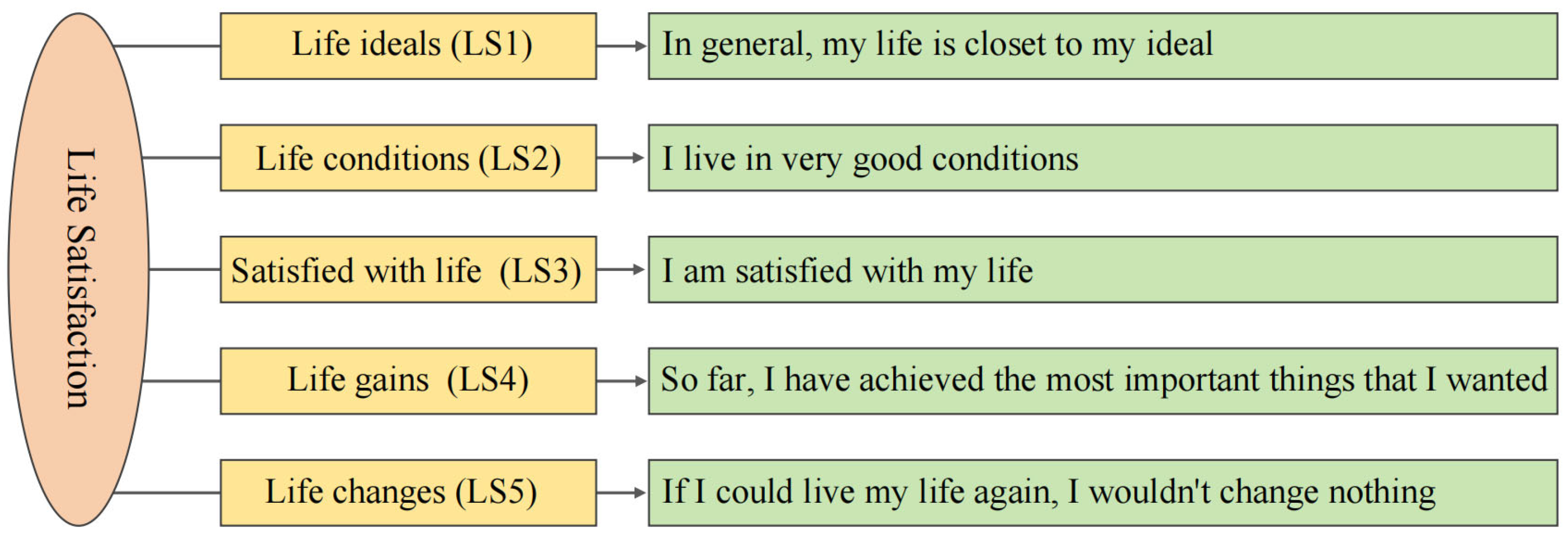
Based on the constructed analysis model, this study mainly includes two types of variables—life satisfaction as the dependent variable, and the independent variables, which encompass the housing environment, neighborhood environment, community environment characteristics, as well as demographic and socio-economic characteristics, and optimistic personality. Table 1 reports the characteristics of demographic and socio-economic attributes (Table 1). It is worth noting that literature research has proven that an optimistic personality has an impact on life satisfaction [38,39]. However, this relationship is seldom explored in urban planning research, so this study incorporates the concept of optimism. The measurement of the optimistic personality trait uses the revised Life Orientation Test, LOT-R [55], which is a widely accepted measure known for its reliability and validity. The literature research divides this scale into optimistic and pessimistic factors [56] or a single optimistic factor [57]. This study focuses solely on three items representing the optimistic factor from the aforementioned literature: “Under uncertain circumstances, I often expect the best results (LOTR1)”, “I am optimistic about my future (LOTR2)”, “Overall, I expect good things rather than bad things to happen to me (LOTR3)”. The dependent variable, life satisfaction, is measured using the Satisfaction with Life Scale (SWLS) developed by Diener [58], which is a widely utilized tool known for its robust reliability and validity [59]. The SWLS comprises five items that primarily measure “Life ideals (LS1)”, “Life conditions (LS2)”, “Satisfied with life (LS3)”, “Life gains (LS4) “, and “Life changes (LS5)” (Figure 3).
The first dimension of the variable is the evaluation of the neighborhood housing environment, aimed at examining the respondents’ real perception and evaluation of the housing environment. This part includes six items: “Degree of satisfaction with the ventilation conditions of the current housing (HE1)”, “Degree of satisfaction with the lighting conditions of the current housing (HE2)”, “Degree of satisfaction with the corridor environment of the current housing (HE3)”, “Degree of satisfaction with the construction quality of the current housing (HE4)”, “Degree of satisfaction with the appearance of the current housing construction (HE5)”, and “Degree of satisfaction with the layout of the current housing (HE6)”; the higher the score of each item, the better the evaluation of the residents of the housing environment aspect.
The second dimension of the variable is the evaluation of the neighborhood environment, aimed at examining the respondents’ real perception and evaluation of the neighborhood environment where they live. This part includes six items: “Degree of satisfaction with the quietness of the neighborhood area (no noise) (NE1)”, “Degree of satisfaction with the sanitation environment of the neighborhood area (NE2)”, “Degree of satisfaction with the leisure sports and fitness facilities of the neighborhood area (NE3)”, “Degree of satisfaction with the parking facilities of the neighborhood area (NE4)”, “Degree of satisfaction with the landscape and road lighting facilities of the neighborhood area (NE5)”, and “Degree of satisfaction with the property management services of the neighborhood area (NE6)”. The higher the score for each item, the better the evaluation of the residents of the neighborhood environment aspect. The variables mentioned above, including optimistic personality, life satisfaction, housing scale, and neighborhood scale environment, were assessed using a Likert scale ranging from “1-strongly disagree” to “7-strongly agree” to gauge the respondents’ perceptions of each item.
The third dimension of the variable is the community’s built environment. After the survey is completed, according to common practices, the spatial information is reverse-coded, and the neighborhood community is converted into geographical coordinates for objective data collection [60], such that the samples with spatial association in the processing of built environment and subjective well-being data can derive better estimates [61]. The study refers to the design of related studies and sets a buffer zone with a radius of 1000 m as the range of the surveyed community for objective built environment measurement calculation (Table 2), including variables reflecting density characteristics such as population density (PD) and building density (BD), functional mix diversity (FMD), road intersection density (RID), bus line density (BLD), bus stop density (BSD) and POI point density (POID). The basic data used in the study mainly come from websites such as Worldpop, Open Street Map, Amap, and Baidu maps.

3.3. Reliability and Validity Testing

Before empirical research, it is essential to assess the reliability and validity of the research instruments to ensure that they accurately capture the intended concepts and content [62]. Reliability focuses on the stability and consistency of the tool’s measurement concepts, facilitating the evaluation of the measurement’s goodness [63]. According to previous research, a Cronbach’s α coefficient above 0.8 indicates good tool reliability, and above 0.7 indicates acceptable reliability, which can be used for further analysis [64].
This study initially conducts factor analysis on the dependent variable, life satisfaction. The Bartlett spherical test yielded a significant chi-square value of approximately 1359.509, and the KMO value is 0.881, indicating good validity and allowing for the following factor analysis. Extracting a single factor accounted for 67.358% of the total variance [64], which meets the relevant standards. After reliability testing, the Cronbach’s α of LS was revealed to be 0.877. The Cronbach’s α of optimistic personality was 0.813, indicating the good internal consistency of the scale. The Bartlett spherical test revealed a statistically significant chi-square value of approximately 2136.103, with a KMO value of 0.916 for evaluating the housing environment. Similarly, the significant chi-square value of approximately 1805.207 and a KMO value of 0.883 for evaluating the neighborhood environment indicate suitability for factor analysis [64,65]. In order to more clearly understand the relationship between housing and neighborhood environment variables and life satisfaction, three factors were extracted separately, with a total explanation of the variation of 84.528% and 82.987%. This indicates that the information in the problem can be extracted effectively, and the validity is good. Consequently, the variables of the housing environment evaluation are divided into three factors—Housing Natural Environment Evaluation (HNEE), Housing Construction Environment and Quality Evaluation (HCEQE), and Housing Layout and Design Evaluation (HLDE)—demonstrating high reliability with a Cronbach’s α of 0.801. The variables of the neighborhood environment evaluation are divided into three factors—Neighborhood Environment Comfort Evaluation (NECE), Neighborhood Facilities Evaluation (NFE), and Neighborhood Property Management and Service Evaluation (NPMSE)—demonstrating high reliability with a Cronbach’s α of 0.795.

3.4. Model Specification

To examine the incremental contribution of built environment variables at different scales, we employed a hierarchical multiple regression analysis. Life satisfaction (LS) served as the dependent variable across all models. The general form of the hierarchical regression model is as follows:
L S i = β 0 + β 1 O P T i + s = 1 S β s S E s , i + e = 1 E β e B E e , i + ϵ i
Here, S E denotes the socio-economic control vector and B E denotes the built-environment vector measured at the housing, neighborhood, or community scale. Specifically:
L S i represents the life satisfaction score for individual i ;
β 0 represents the intercept term;
O P T i represents the optimistic personality score for individual i as a control variable;
S E s , i represents a vector of control variables ( s = 1 , , S ) including age, gender, marital status, occupation, education level, and monthly income for individual i ;
B E e , i represents a vector of built environment variables ( e = 1 , , E ) at the housing, neighborhood, or community scale for individual i ;
β 1 , β s , and β e represent the regression coefficients to be estimated;
ϵ i represents the random error term.
The models were constructed in the following sequence to isolate the effects of variables from proximate to distal scales.
Model 1 (individual and housing scale):
L S i = β 0 + β 1 O P T i + s = 1 6 β s S E s , i + h = 1 4 β h ( H ) H E h , i + ϵ i
In this model, H E h , i represents the vector of housing-scale variables (denoted by superscript ( H ) ). Model 1 controls for respondents’ socio-economic characteristics ( S E s , i ) and optimistic personality ( O P T i ), while introducing all housing-scale environmental variables. The housing scale variables include Housing Natural Environment Evaluation (HNEE), Housing Construction Environment and Quality Evaluation (HCEQE), Housing Layout and Design Evaluation (HLDE), and Per Capita Housing Area (HAPC).
Model 2 (adding neighborhood scale):
L S i = β 0 + β 1 O P T i + s = 1 6 β s S E s , i + h = 1 4 β h ( H ) H E h , i + n = 1 3 β n ( N ) N E n , i + ϵ i
In this model, N E n , i represents the vector of neighborhood scale variables (denoted by superscript ( N ) ). Building upon Model 1, Model 2 adds the neighborhood-scale variables. The neighborhood variables include Neighborhood Environmental Comfort Evaluation (NECE), Neighborhood Facilities Evaluation (NFE), and Neighborhood Property Management and Service Evaluation (NPMSE).
Model 3 (adding community scale):
L S i = β 0 + β 1 O P T i + s = 1 6 β s S E s , i + h = 1 4 β h ( H ) H E h , i + n = 1 3 β n ( N ) N E n , i + c = 1 7 β c ( C ) C E c , i + ϵ i
In this model, C E c , i represents the vector of community-scale variables (denoted by superscript ( C ) ). Finally, Model 3 incorporates all previous variables and further adds the objective community scale variables. The community scale variables include population density (PD), building density (BD), functional mix diversity (FMD), road intersection density (RID), bus line density (BLD), bus stop density (BSD), and point of interest density (POID).
All environmental variables at the housing, neighborhood, and community scales are defined in detail in Table 2. This hierarchical approach enables the examination of whether adding each subsequent set of environmental variables (from housing to neighborhood to community) provides a statistically significant improvement in explaining the variance in life satisfaction beyond the previous model. The improvement in model fit was assessed by examining the change in R-squared (ΔR2) and its associated F-test significance level.

4. Results

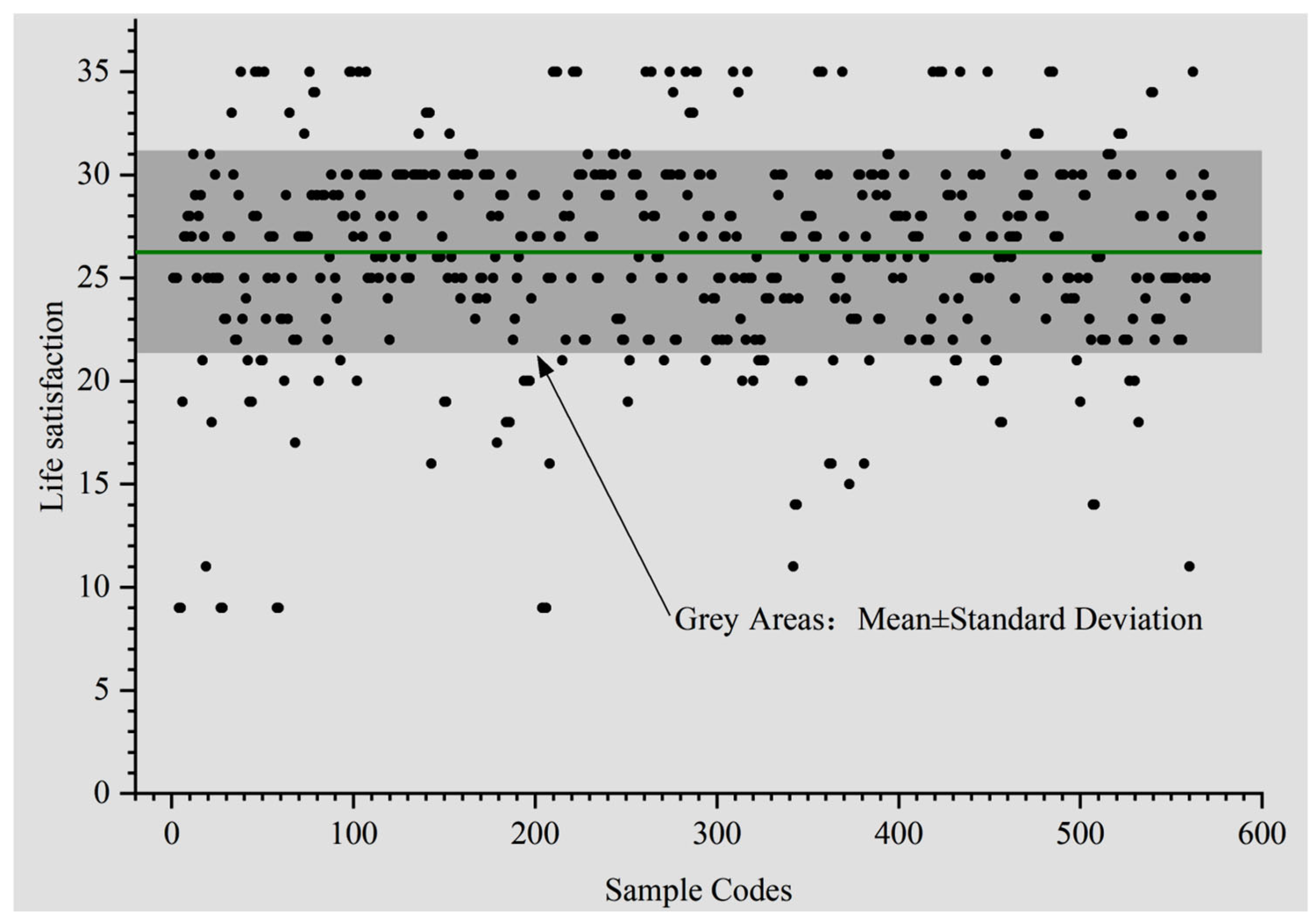
Before model testing, the life satisfaction measurement results are here presented. The cumulative score of the 5 items is 26.283, suggesting a predominantly positive assessment of life satisfaction among the residents (Figure 4). The item means range from 4.910 to 5.520, with skewness ranging from −1.216 to −0.594, and kurtosis ranging from 0.218 to 1.740. These values indicate that the distribution of scores approximates a normal distribution [62], supporting the subsequent model analysis [66].
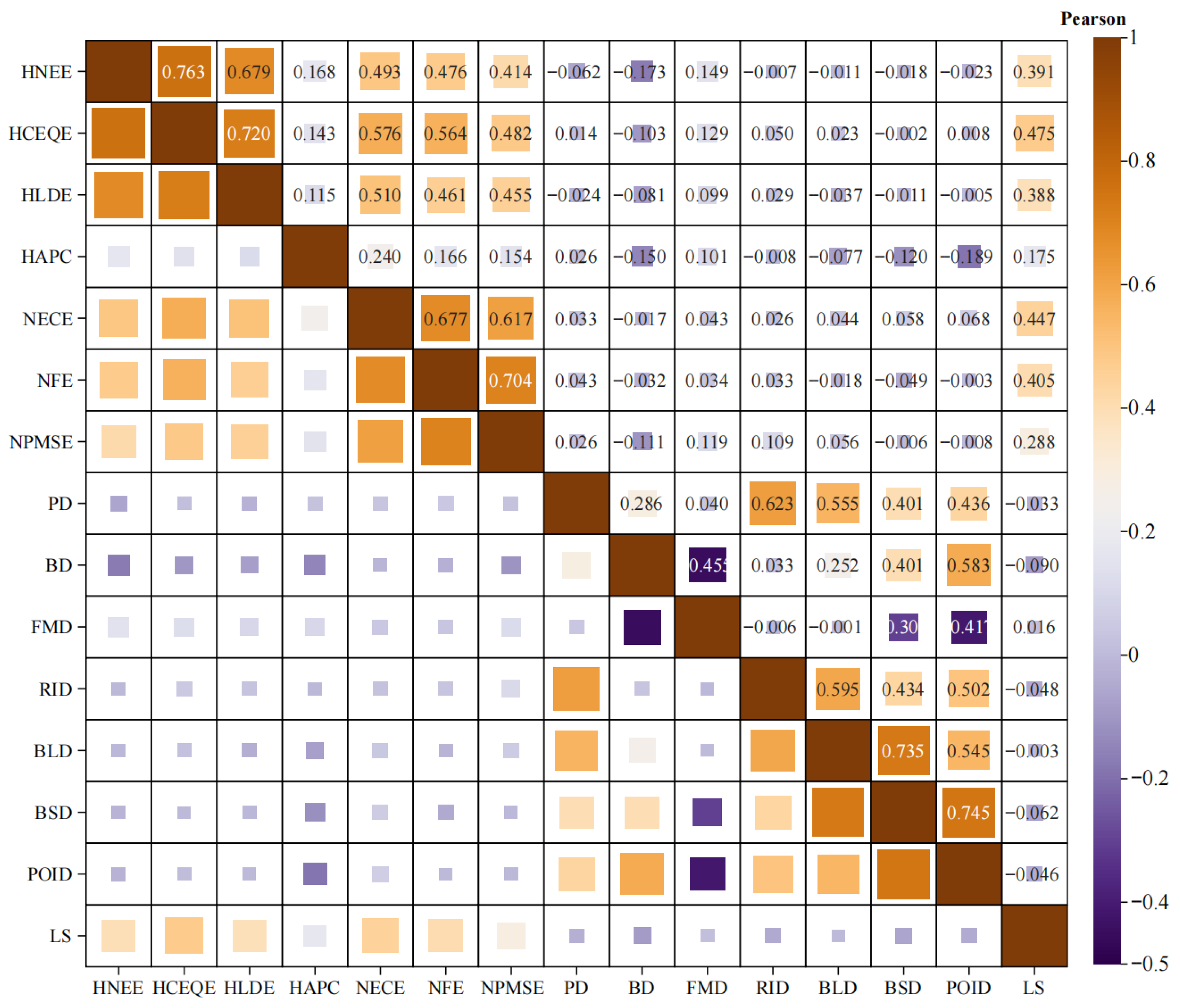
The study uses hierarchical regression analysis to explore the impact of multi-scale environments on LS. Before conducting the model analysis, the study examined the correlation between the primary independent variables and life satisfaction. Additionally, Figure 5 shows the correlation heat map analysis of the relationship between the factors at the housing, neighborhood and community scales, and LS. Furthermore, prior to the analysis, the study assesses the fundamental assumptions of the regression model. The study has successively tested the linear correlation assumption, zero mean assumption, and normality assumption of the model, and the results show that there is no obvious violation of the aforementioned assumptions.
The results of the hierarchical regression analysis, constructed as specified in Section 3.4, are presented in Table 3. Model 1, which includes socio-economic characteristics, optimistic attitude, and housing-scale environmental variables, explains a significant proportion of variance in life satisfaction (LS) (R2 = 0.381, Adjusted R2 = 0.368). The sequential addition of neighborhood-scale variables in Model 2 and community-scale (“5D”) variables in Model 3 significantly improved model fit, as evidenced by the increases in Adjusted R2 (to 0.384 and 0.398, respectively) and significant ΔR2 values (0.018 and 0.014, both p < 0.01). This progressive enhancement confirms that multi-scale environmental factors collectively strengthen the explanatory power for LS.
Specifically, in Model 1, both Housing Construction Environment and Quality Evaluation (HCEQE) (β = 0.332, p < 0.001) and Per Capita Housing Area (HAPC) (β = 0.090, p < 0.05) exerted significant positive effects on LS, supporting Hypothesis 1. The standardized coefficients indicate a greater contribution of HCEQE than HAPC. Model 2 introduced neighborhood-scale variables. Among these, Neighborhood Environmental Comfort Evaluation (NECE) (β = 0.112, p < 0.05) and Neighborhood Facilities Evaluation (NFE) (β = 0.142, p < 0.01) were positively associated with LS, whereas Neighborhood Property Management and Service Evaluation (NPMSE) (β = −0.128, p < 0.01) exhibited a significant negative impact. The contribution of NFE was substantially greater than that of NECE and NPMSE. Model 3 incorporated community-scale built environment factors. Bus line density (BLD) (β = 0.177, p < 0.01) showed a significant positive effect on LS. In contrast, building density (BD) (β = −0.091, p < 0.10), functional mix diversity (FMD) (β = −0.085, p < 0.05), road intersection density (RID) (β = −0.136, p < 0.01), and bus stop density (BSD) (β = −0.134, p < 0.05) were negatively associated with LS. The contribution of BLD was substantially greater than that of other community-scale factors.
Overall, the results demonstrate the robust and multifaceted impact of the built environment on LS across three spatial scales. Given that Model 3 offers the most comprehensive explanation, the following discussion will focus on its results. In summary, the results substantiate all three hypotheses of this study. Given that Model 3 demonstrates the highest explanatory power, the following section focuses on the results of Model 3 for detailed analysis and discussion.

5. Discussion

This study employed a hierarchical regression model to systematically examine the differential effects of the built environment on residents’ life satisfaction (LS) across three spatial scales: housing, neighborhood, and community. Our findings reveal that the explanatory power of environmental variables on life satisfaction exhibits a diminishing trend from proximate to distal scales (housing → neighborhood → community). This observed scaling pattern intriguingly resonates with the theoretical propositions of fractal urban theory. Cities are recognized as complex systems exhibiting fractal characteristics, with structural and functional patterns repeating across scales [67,68]. Our results align with this view, suggesting that the built environment elements influencing residents’ subjective well-being also demonstrate significant scale-dependent effects, where the immediate, micro-scale personal living domain (housing) exerts a far greater influence than the macro-scale community structural features. Several specific findings warrant in-depth interpretation.
First, the observed negative association between the evaluation of property management services (NPMSE) and LS, though counterintuitive, can be explained through integrated theoretical lenses. Drawing on Expectation Confirmation Theory [69], higher service fees can elevate residents’ expectations. A perceived shortfall between expected and actual service quality can generate significant disappointment, thereby negatively impacting overall life evaluations. Furthermore, from a behavioral economics perspective, the financial burden imposed by high service costs can act as a strain on household budgets, potentially diminishing the positive utility derived from disposable income and adversely affecting life satisfaction [70]. Additionally, socio-economic heterogeneity within communities can lead to divergent perceptions of value fairness. If residents perceive a mismatch between high costs and the services received, which may not align with their specific needs, a sense of inequity can arise, ultimately influencing overall life appraisal [71].
Second, the identified negative correlation between bus stop density (BSD) and LS contrasts with the conventional planning wisdom that increased accessibility invariably enhances well-being. A plausible explanation lies in the environmental externalities concomitant with high-density bus stop density, including noise, air pollution, visual clutter, and safety risks, which may outweigh the benefits of accessibility [7]. Critically, the simultaneous inclusion of both bus stop density (BSD) and bus line density (BLD) in the model introduces a statistical challenge—multicollinearity. While the Variance Inflation Factor (VIF) was within acceptable limits, it remains difficult to entirely disentangle their independent effects [72]. BSD likely serves as a more direct proxy for localized nuisances (e.g., passenger congregation, frequent vehicle idling and acceleration), whereas BLD reflects the broader environmental load of the traffic corridor. Consequently, the negative coefficient for BSD may capture the environmental negatives associated with high-density bus stops. This finding suggests that the traditional ‘5D’ framework might need refinement to better disentangle the ‘benefit’ (accessibility) and ‘cost’ (environmental burden) dimensions of transit density.
Furthermore, our study contributes to a growing body of literature seeking to understand the perceptual and cognitive mechanisms through which residents evaluate the built environment. Emerging methodologies, such as eye-tracking, are being employed to uncover the attentional mechanisms underpinning environmental perception [73,74,75]. Research in this area suggests that individuals may exhibit rapid ‘vigilance–avoidance’ patterns toward negative environmental cues (e.g., disorder, crowding), while demonstrating sustained attention toward positive features (e.g., greenery, engaging urban furniture). This neuroscientific perspective provides a plausible mechanistic underpinning for our findings: negative evaluations of property services (potentially triggered by vigilance toward negative cues) and the perception of potentially adverse features in high-density transit environments could influence overall life satisfaction judgments through automated, subconscious cognitive pathways.

6. Conclusions and Recommendations

6.1. Conclusions

To examine the impact of multi-scale environments on LS, this study employed a hierarchical regression analysis to assess the explanatory power of LS following the incorporation of housing, neighborhood, and community environments. The study found that built environments at different scales affect life satisfaction, and reached the following conclusions:
(1)
The explanatory power of the model for the dependent variable gradually increases with the increase in environmental variables such as housing, neighborhood, and community, after controlling the other variables. Notably, the results demonstrate that the explanatory ability has a hierarchical structure, and the housing environment shows the largest increase in explanatory ability, followed by the neighborhood environment, and finally the community environment;
(2)
In terms of the housing environment, the Housing Construction Environment and Quality Evaluation (HCEQE) and per capita housing area (HAPC) have a significant impact on residents’ life satisfaction, after controlling for other variables;
(3)
In terms of the neighborhood environment, the comfortable evaluation of the neighborhood environment (NECE) and facility evaluation (NFE) at the neighborhood scale significantly affect life satisfaction, while the property management and service evaluation (NPMSE) have significant negative impacts.
(4)
In terms of the community environment, building density (BD), functional mix density (FMD), road intersection density (RID), bus stop density (BSD), and bus line density (BLD) all significantly affect life satisfaction.

6.2. Theoretical and Practical Implications

Theoretically, this study not only validates the effectiveness of a multi-scale analytical framework for understanding the relationship between the built environment and resident well-being, but also, by engaging with fractal urban theory and environmental perception research, emphasizes the need for future research to pay greater attention to the scalar interconnections of urban form and the psychological mechanisms of the attentional processing of environmental information.
Practically, this research offers the following insights for urban planning and design aimed at enhancing residents’ life satisfaction:
(1)
Housing Scale—Greater emphasis should be placed on construction quality, architectural aesthetics, and interior layout design in housing development. Real estate policies should be optimized to guide housing prices within a reasonable range and increase per capita living space;
(2)
Neighborhood Scale—Planning and design should prioritize neighborhood environmental comfort (e.g., noise reduction, sanitation) and optimize the allocation of facilities such as leisure sports and fitness facilities, landscape and road lighting facilities, and parking facilities. Particular attention must be paid to carefully assessing the alignment between the content of property services and their fees. Enhancing service transparency and perceived fairness is crucial to avoid undermining resident well-being due to excessive financial burdens or perceived lack of value;
(3)
Community Scale—The urban planners and managers should focus on optimizing building density, reasonably planning functional configurations, and strengthening road intersection design. The planning of mixed-use developments and the deployment of public transport infrastructure must involve meticulous environmental impact assessment and urban design. The focus should be on mitigating potential negative externalities—such as noise, pollution, and safety risks—through design interventions (e.g., sound barriers, green buffer zones, rational stop layout). The goal is to realize the true life-enhancing benefits of Transit-Oriented Development (TOD) models, moving beyond merely pursuing density metrics. In addition, considering the important role of personality, it is necessary to establish a multi-dimensional propaganda system of “government–community–school–family” to promote the formation of an optimistic personality, and to enhance the subjective well-being and life satisfaction level of residents.

6.3. Research Limitions and Future Research Directions

This study examined the effects of the built environment on life satisfaction at three spatial scales—housing, neighborhood, and community—and yielded valuable findings, while also revealing limitations and directions for future research. First, the use of multiple regression methods allows us to identify associations between independent variables and life satisfaction, but prevents causal inference. Second, due to data constraints, the built environment was analyzed only at the housing, neighborhood, and community scales, omitting potential effects at the city scale. Moving forward, future research could be enhanced by expanding the measures of the built environment—such as perceived walkability, fine-grained spatial connectivity, or accessibility to specific types of services—and studies should adopt longitudinal or natural experimental designs to strengthen causal claims regarding the impact of built environments on subjective well-being. Furthermore, integrating more objective measurement techniques—such as eye-tracking, virtual reality experiments, and mobile sensors—could capture real-time physiological and behavioral responses, helping to elucidate underlying mediating mechanisms. Furthermore, while this study provides insights from a major Chinese city undergoing rapid urbanization, the generalizability of the findings to other cities with different developmental stages, cultural contexts, or urban forms (both within China and internationally) may be limited. Research should also expand to macro-scale urban structures (e.g., polycentricity, city size) and examine how they interact with local features to influence resident well-being. Finally, interdisciplinary approaches combining urban planning, environmental psychology, public health, and complexity science (e.g., fractal and network analysis) are needed to develop more comprehensive theoretical models of human–environment interactions and well-being.

Author Contributions

H.L., conceptualization; writing—original draft; writing—review and editing. C.P., writing—original draft; validation; investigation. N.Q., writing—review and editing; visualization. J.G., writing—review; supervision; validation; data curation; resources. J.W., writing—review and editing; software. All authors have read and agreed to the published version of the manuscript.

Funding

This research was funded by (1) Guangdong Philosophy and Social Science Planning Project (GD24XSH06, GD24XYS018), (2) Projects of Talents Recruitment of GDUPT (2023rcyj2015), (3) Projects of PhDs’ Start-up Research of GDUPT (2023bsqd1008, 2022bsqd2004), (4) Science and Technology Programme of Maoming of Guangdong Province of China (2023398, 2023411, 2024055, 2024061).

Data Availability Statement

The datasets used and/or analyzed during the current study are available from the corresponding author on reasonable request.

Conflicts of Interest

The authors declare no potential conflicts of interest with respect to the research, authorship, and/or publication of this article.

References

  1. Yang, J.; Tao, Y.; Liu, Z.; Li, M.; Liu, J. The impact of neighborhood effects on community interaction and life satisfaction: A multi-level path analysis based on 26 community residents in Beijing. Hum. Geogr. 2021, 36, 27–34. [Google Scholar]
  2. Diener, E. (Ed.) The Science of Well-Being: The Collected Works of Ed Diene; Springer Science & Business Media: Berlin/Heidelberg, Germany, 2009; Volume 37. [Google Scholar]
  3. Diener, E.; Chan, M.Y. Happy people live longer: Subjective well-being contributes to health and longevity. Appl. Psychol. Health Well-Being 2011, 3, 1–43. [Google Scholar] [CrossRef]
  4. Zhan, D.; Zhang, W.; Yu, J.; Miao, C.; Liu, C. The spatial characteristics and mechanisms of urban livability based on objective evaluation: A case study of Beijing. Reg. Res. Dev. 2016, 35, 68–73. [Google Scholar]
  5. Brockmann, H.; Delhey, J.; Welzel, C.; Yuan, H. The China puzzle: Falling happiness in a rising economy. J. Happiness Stud. 2009, 10, 387–405. [Google Scholar] [CrossRef]
  6. Ma, J.; Liu, G.; Rao, J. Progress in the study of the impact of geographical environment and spatiotemporal behavior on subjective well-being. Prog. Geogr. 2022, 41, 718–730. [Google Scholar] [CrossRef]
  7. Cao, X.J. How does neighborhood design affect life satisfaction? Evidence from Twin Cities. Travel Behav. Soc. 2016, 5, 68–76. [Google Scholar] [CrossRef]
  8. Yuan, Y.; Ding, K.; Cao, X.; Zhu, Y.; Zhang, Y. A review of research methods on community satisfaction and influencing factors. Urban Dev. Stud. 2018, 25, 105–111. [Google Scholar]
  9. Mouratidis, K. Rethinking how built environments influence subjective well-being: A new conceptual framework. J. Urban. Int. Res. Placemaking Urban Sustain. 2018, 11, 24–40. [Google Scholar] [CrossRef]
  10. Fried, M. The structure and significance of community satisfaction. Popul. Environ. 1984, 7, 61–86. [Google Scholar] [CrossRef]
  11. Liu, X.; Wang, Z.; Song, J.; Liu, C.; Deng, M. The impact of residential environment on residents’ subjective well-being: An example from mixed residential communities in Shenzhen. Prog. Geogr. 2022, 41, 2099–2107. [Google Scholar] [CrossRef]
  12. Lee, S.M.; Conway, T.L.; Frank, L.D.; Cain, K.L.; Sallis, J.F. The relation of perceived and objective environment attributes to neighborhood satisfaction. Environ. Behav. 2017, 49, 136–160. [Google Scholar] [CrossRef]
  13. Kang, L.; Zhang, W. Influence of neighborhood social environment on residents’ well-being: A case study of typical low-income communities in Beijing city. Areal Res. Dev. 2021, 40, 50–55. [Google Scholar]
  14. Batson, C.D.; Monnat, S.M. Distress in the desert: Neighborhood disorder, resident satisfaction, and quality of life during the Las Vegas foreclosure crisis. Urban Aff. Rev. 2015, 51, 205–238. [Google Scholar] [CrossRef] [PubMed]
  15. Friedman, D.; Parikh, N.S.; Giunta, N.; Fahs, M.C.; Gallo, W.T. The influence of neighborhood factors on the quality of life of older adults attending New York City senior centers: Results from the Health Indicators Project. Qual. Life Res. 2012, 21, 123–131. [Google Scholar] [CrossRef]
  16. Huang, Y.; He, L. Urbanization, environmental pollution and subjective well-being: An empirical study on China. China Soft Sci. 2013, 12, 82–93. [Google Scholar]
  17. Sun, B.; Yin, C. Relationship between multi-scale urban built environments and body mass index: A study of China. Appl. Geogr. 2018, 94, 230–240. [Google Scholar] [CrossRef]
  18. Han, H.; Yang, K.; Yang, C.; Yang, G.; Xu, L. Influence and Mechanism of a Multi-Scale Built Environment on the Leisure Activities of the Elderly: Evidence from Hefei City in China. Int. J. Environ. Res. Public Health 2022, 19, 9237. [Google Scholar] [CrossRef]
  19. Yin, C.; Shao, C.; Dong, C.; Wang, X. Happiness in urbanizing China: The role of commuting and multi-scale built environment across urban regions. Transp. Res. Part D Transp. Environ. 2019, 74, 306–317. [Google Scholar] [CrossRef]
  20. Cao, X.; Wu, X.; Yuan, Y. Examining built environmental correlates of neighborhood satisfaction: A focus on analysis approaches. J. Plan. Lit. 2018, 33, 419–432. [Google Scholar] [CrossRef]
  21. Diener, E. Subjective well-being: The science of happiness and a proposal for a national index. Am. Psychol. 2000, 55, 34–43. [Google Scholar] [CrossRef] [PubMed]
  22. Ryan, R.M.; Deci, E.L. On happiness and human potentials: A review of research on hedonic and eudaimonic well-being. Annu. Rev. Psychol. 2001, 52, 141–166. [Google Scholar] [CrossRef]
  23. Pavot, W.; Diener, E. The satisfaction with life scale and the emerging construct of life satisfaction. J. Posit. Psychol. 2008, 3, 137–152. [Google Scholar] [CrossRef]
  24. Ryff, C.D. Happiness is everything, or is it? Explorations on the meaning of psychological well-being. J. Personal. Soc. Psychol. 1989, 57, 1069. [Google Scholar] [CrossRef]
  25. Kennes, A.; Peeters, S.; Janssens, M.; Goedhart, R.; Myin-Germeys, I.; Bastiaansen, T. Optimism and mental health in adolescence: A prospective validation study of the Dutch Life-Orientation Test-Revised (LOT-RA) for adolescents. Psychol. Belg. 2021, 61, 104–115. [Google Scholar] [CrossRef] [PubMed]
  26. Oishi, S. The psychology of residential mobility: Implications for the self, social relationships, and well-being. Perspect. Psychol. Sci. 2010, 5, 5–21. [Google Scholar] [CrossRef]
  27. Lin, X.; Yang, J. A review of the relationship between built environment and public health in North American metropolitan areas and its implications. Planner 2015, 31, 12–19. [Google Scholar]
  28. Uppal, S. Impact of the timing, type and severity of disability on the subjective well-being of individuals with disabilities. Soc. Sci. Med. 2006, 63, 525–539. [Google Scholar] [CrossRef]
  29. Jivraj, S.; Nazroo, J.; Vanhoutte, B.; Chandola, T. Aging and subjective well-being in later life. J. Gerontol. Ser. B Psychol. Sci. Soc. Sci. 2014, 69, 930–941. [Google Scholar] [CrossRef]
  30. Lamu, A.N.; Olsen, J.A. The relative importance of health, income and social relations for subjective well-being: An integrative analysis. Soc. Sci. Med. 2016, 152, 176–185. [Google Scholar] [CrossRef]
  31. Stutzer, A.; Frey, B.S. Recent advances in the economics of individual subjective well-being. Soc. Res. Int. Q. 2010, 77, 679–714. [Google Scholar] [CrossRef]
  32. Mhaoláin, A.M.N.; Gallagher, D.; Connell, H.O.; Chin, A.V.; Bruce, I.; Hamilton, F.; Teehee, E.; Coen, R.; Coakley, D.; Cunningham, C.; et al. Subjective well-being amongst community-dwelling elders: What determines satisfaction with life? Findings from the Dublin Healthy Aging Study. Int. Psychogeriatr. 2012, 24, 316–323. [Google Scholar] [CrossRef]
  33. Yu, Y.; Hu, Y. International research progress on the health impact of community built environment based on physical activity research perspective: A literature review and thoughts. Archit. J. 2017, 2, 33–38. [Google Scholar]
  34. Cervero, R.; Kockelman, K. Travel demand and the 3Ds: Density, diversity, and design. Transp. Res. Part D Transp. Environ. 1997, 2, 199–219. [Google Scholar] [CrossRef]
  35. Ewing, R.; Cervero, R. Travel and the built environment: A meta-analysis. J. Am. Plan. Assoc. 2010, 76, 265–294. [Google Scholar] [CrossRef]
  36. Srinivasan, S.; O’fallon, L.R.; Dearry, A. Creating healthy communities, healthy homes, healthy people: Initiating a research agenda on the built environment and public health. Am. J. Public Health 2003, 93, 1446–1450. [Google Scholar] [CrossRef] [PubMed]
  37. Dang, Y.; Yu, J.; Zhang, W.; Gao, S.; Wang, J. Evaluation and influencing factors of urban residential environment satisfaction in the Bohai Rim region. Prog. Geogr. 2016, 35, 184–194. [Google Scholar]
  38. Wei, Z.; Zhen, F.; Qin, X. Study on the quality of living environment and institutional influencing factors in Guangzhou’s affordable housing communities. Geogr. Sci. 2020, 40, 89–96. [Google Scholar]
  39. Arellana, J.; Saltarín, M.; Larrañaga, A.M.; González, V.I.; Henao, C.A. Urban walkability considering pedestrians’ perceptions of the built environment: A 10-year review and a case study in a medium-sized city in Latin America. Transp. Rev. 2020, 40, 183–203. [Google Scholar] [CrossRef]
  40. Campbell, A.; Converse, P.E.; Rodgers, W.L. The Quality of American Life: Perceptions, Evaluations, and Satisfactions; Russell Sage Foundation: New York, NY, USA, 1976. [Google Scholar]
  41. Sirgy, M.J.; Cornwell, T. How neighborhood features affect quality of life. Soc. Indic. Res. 2002, 59, 79–114. [Google Scholar] [CrossRef]
  42. Liu, Y.; Pan, Z.; Feng, J.; Li, Y.; He, S. Factors affecting emotional well-being of residents in low-rent housing in metropolises in China: A case study of Guangzhou. Trop. Geogr. 2019, 39, 180–187. [Google Scholar] [CrossRef]
  43. Li, Z. A study on residential satisfaction in “new immigrant” settlements in Chinese cities: A case study of Beijing, Shanghai, and Guangzhou. Urban Plan. 2011, 35, 75–82. [Google Scholar]
  44. Dekker, K.; De Vos, S.; Musterd, S.; Van Kempen, R. Residential satisfaction in housing estates in European cities: A multi-level research approach. Hous. Stud. 2011, 26, 479–499. [Google Scholar] [CrossRef]
  45. Liu, X.; Yu, Y. The impact of community built environment on the health of the elderly under high-density living conditions and intervention pathways. Urban Dev. Stud. 2023, 30, 35–42. [Google Scholar]
  46. Han, S. Social capital and subjective happiness: Which contexts matter? J. Happiness Stud. 2015, 16, 241–255. [Google Scholar] [CrossRef]
  47. Lin, J.; Sun, B. The impact of the built environment on the subjective well-being of urban residents: Evidence from the China Labor Dynamics Survey. Urban Dev. Stud. 2017, 24, 69–75. [Google Scholar]
  48. Melis, G.; Gelormino, E.; Marra, G.; Ferrero, G.; Costa, G. The effects of the urban built environment on mental health: A cohort study in a large northern Italian city. Int. J. Environ. Res. Public Health 2015, 12, 14898–14915. [Google Scholar] [CrossRef]
  49. Mason, S.G. Can community design build trust? A comparative study of design factors in Boise, Idaho neighborhoods. Cities 2010, 27, 456–465. [Google Scholar] [CrossRef]
  50. Cao, J. The association between light rail transit and satisfactions with travel and life: Evidence from Twin Cities. Transportation 2013, 40, 921–933. [Google Scholar] [CrossRef]
  51. Ma, J.; Dong, G.; Chen, Y.; Zhang, W.; Li, T. Does a satisfactory neighborhood environment lead to a satisfying life? An investigation of the association between neighborhood environment and life satisfaction in Beijing. Cities 2018, 74, 229–239. [Google Scholar] [CrossRef]
  52. Bardo, A.R. A life course model for a domains-of-life approach to happiness: Evidence from the United States. Adv. Life Course Res. 2017, 33, 11–22. [Google Scholar] [CrossRef]
  53. Su, L.; Zhou, S. The impact of neighborhood environment on happiness under the background of residential mobility: Differences across life course stages. Prog. Geogr. 2021, 40, 1344–1354. [Google Scholar] [CrossRef]
  54. Liu, Y.; Xiao, T.; Liu, Y.; Song, Y.; Li, Z. The impact of urban built environment on the happiness of residents in Guangzhou City: An analysis based on 15-min walkable range. Prog. Geogr. 2020, 39, 1270–1282. [Google Scholar] [CrossRef]
  55. Scheier, M.F.; Carver, C.S.; Bridges, M.W. Distinguishing optimism from neuroticism (and trait anxiety, self-mastery, and self-esteem): A reevaluation of the Life Orientation Test. J. Pers. Soc. Psychol. 1994, 67, 1063–1078. [Google Scholar] [CrossRef] [PubMed]
  56. Wen, Z. The reliability and validity of the Life Orientation Test in college students. Chin. J. Ment. Health 2012, 26, 305–309. [Google Scholar]
  57. Gu, H.; Wang, C. Statistical control of item wording effects: An example of the Chinese version of the Life Orientation Test. Psychol Sci. 2012, 35, 1247–1253. [Google Scholar]
  58. Diener, E.; Emmons, R.A.; Larsen, R.J.; Griffin, S. The satisfaction with life scale. J. Pers. Assess. 1985, 49, 71–75. [Google Scholar] [CrossRef]
  59. Feng, J.; Tang, S.; Chuai, X. The impact of neighborhood environments on the quality of life of elderly people: Evidence from Nanjing, China. Urban Stud. 2018, 55, 2020–2039. [Google Scholar] [CrossRef]
  60. Johnson, B.T.; Cromley, E.K.; Marrouch, N. Spatiotemporal meta-analysis: Reviewing health psychology phenomena over space and time. Health Psychol. Rev. 2017, 11, 280–291. [Google Scholar] [CrossRef] [PubMed]
  61. Grafström, A.; Tillé, Y. Doubly balanced spatial sampling with spreading and restitution of auxiliary totals. Environmetrics 2013, 24, 120–131. [Google Scholar] [CrossRef]
  62. Hair, J.F.; Money, A.H.; Samouel, P.; Page, M. Research methods for business. Educ. + Train. 2007, 49, 336–337. [Google Scholar] [CrossRef]
  63. Sekaran, U.; Bougie, R. Research Methods for Business: A Skill Building Approach, 7th ed.; John Wiley & Sons: Hoboken, NJ, USA, 2016. [Google Scholar]
  64. Hair, J.F., Jr.; Black, W.C.; Babin, B.J.; Anderson, R.E. Multivariate Data Analysis, 7th ed.; Prentice Hall: Upper Saddle River, NJ, USA, 2010. [Google Scholar]
  65. Kline, R.B. Principles and Practice of Structural Equation Modeling; Guilford Publications: New York, NY, USA, 2023; pp. 48–52. [Google Scholar]
  66. Neter, J.; Wasserman, W.; Kutner, M.H. Applied Linear Statistical Models: Regression, Analysis of Variance, and Experimental Designs, 3rd ed.; Irwin: Homewood, IL, USA, 1990. [Google Scholar]
  67. Batty, M.; Longley, P.A. Fractal Cities: A Geometry of Form and Function; Academic Press: Cambridge, MA, USA, 1994. [Google Scholar]
  68. Batty, M. The size, scale, and shape of cities. Science 2008, 319, 769–771. [Google Scholar] [CrossRef]
  69. Oliver, R.L. A cognitive model of the antecedents and consequences of satisfaction decisions. J. Mark. Res. 1980, 17, 460–469. [Google Scholar] [CrossRef]
  70. Kahneman, D.; Deaton, A. High income improves evaluation of life but not emotional well-being. Proc. Natl. Acad. Sci. USA 2010, 107, 16489–16493. [Google Scholar] [CrossRef] [PubMed]
  71. Hur, M.; Morrow-Jones, H. Factors that influence residents’ satisfaction with neighborhoods. Environ. Behav. 2008, 40, 619–635. [Google Scholar] [CrossRef]
  72. Graham, M.H. Confronting multicollinearity in ecological multiple regression. Ecology 2003, 84, 2809–2815. [Google Scholar] [CrossRef]
  73. Sussman, A.; Hollander, J.B. Cognitive Architecture: Designing for How We Respond to the Built Environment; Routledge: Oxfordshire, UK, 2021. [Google Scholar]
  74. Lavdas, A.A.; Salingaros, N.A.; Sussman, A. Visual attention software: A new tool for understanding the “subliminal” experience of the built environment. Appl. Sci. 2021, 11, 6197. [Google Scholar] [CrossRef]
  75. Lavdas, A.A. Eye-tracking applications in architecture and design. Encyclopedia 2024, 4, 1312–1323. [Google Scholar] [CrossRef]
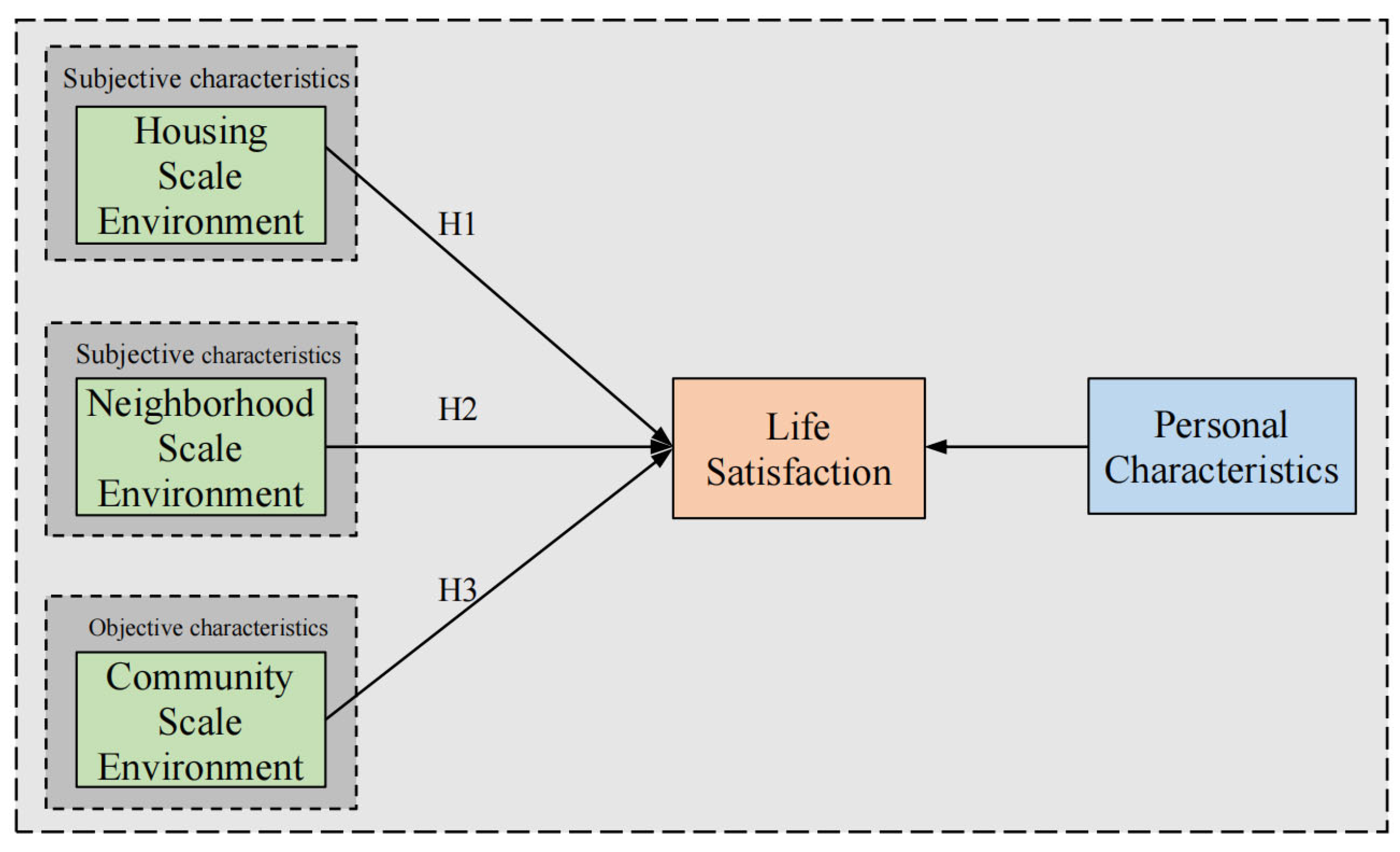
Figure 1. The theoretical framework of the relationship among the housing scale environment, the neighborhood scale environment, the community scale environment, and LS.
Buildings 15 03311 g001
Figure 2. Study areas and the distribution of sample communities.
Buildings 15 03311 g002
Figure 3. The five items of the SWLS.
Buildings 15 03311 g003
Figure 4. The distribution of the total score of life satisfaction.
Buildings 15 03311 g004
Figure 5. Correlation heatmap between variables.
Buildings 15 03311 g005
Table 1. Description of sample characteristics.
VariableTypeFrequencyPercentage (%)
Age18–2919233.803
30–3911420.070
40–497713.556
50–599717.077
≥608815.494
GenderMale29151.232
Female27748.768
MarriageMarried34360.387
Single17731.162
Divorced122.113
Other366.338
OccupationGovernment, Institutions, or Public Service Workers6912.148
Company Employees15927.993
Freelancers14725.880
Retired Persons7913.908
Students315.458
Other8314.613
Education LevelJunior High School or Below12922.711
High School or Technical School14926.232
College or University24643.310
Postgraduate or Above447.747
Monthly Income (RMB)≤500021437.676
5001–800015326.937
8001–10,0007312.852
10,001–13,0006611.620
≥13,0016210.915
Table 2. Description and characteristic statistics of main independent variables.
VariableScaleDescriptionMeanSD
HNEEHousingAverage score of two measurement items for ventilation and lighting conditions of the house5.6761.102
HCEQEHousingAverage score of three measurement items for construction environment, construction quality, and appearance of the building5.4111.147
HLDEHousingScore for the evaluation of the house layout and design5.4171.299
HAPCHousingPer capita housing area 2.7121.625
NECENeighborhoodAverage score of two measurement items for quietness and sanitation environment within the neighborhood area5.1521.303
NFENeighborhoodAverage score of three measurement items for sports and fitness facilities, parking facilities, and landscape lighting facilities5.0601.327
NPMSENeighborhoodScore for the evaluation of property management and services5.1061.495
PDCommunityAverage population number within a 1000 m buffer zone (10,000 people/km2)4.3182.305
BDCommunityRatio of the sum of building base areas to the occupied area within a 1000 m buffer zone0.3110.074
FMDCommunityDiversity of facilities such as hospitals, restaurants, convenience stores, shopping malls, schools, banks, entertainment facilities, tourism facilities, government and institutional facilities, and postal facilities within a 1000 m radius buffer zone, calculated as
M I X = i = 1 n S i   l n S i
In the provided formula, the variable S i represents the proportion of POI belonging to category i relative to the total number of POI within the 1000 m radius buffer. The parameter n represents the total count of unique POI categories encompassed by this buffer.
0.7300.058
RIDCommunityRatio of the number of main road intersections to the geographical unit area within a 1000 m buffer zone (km/km2)143.22472.379
BLDCommunityRatio of the total length of bus lines to the geographical unit area within a 1000 m buffer zone (km/km2)8.4893.169
BSDCommunityRatio of the number of bus stops and subway stations to the geographical unit area within a 1000 m buffer zone (units/km2)9.9182.916
POIDCommunityRatio of the total number of ten types of POI points such as accommodation, catering, shopping, leisure and entertainment, tourism, scientific research and education, government institutions, large shopping, financial services facilities to the geographical unit area within a 1000 m buffer zone (units/km2)361.799211.412
Note: SD represents standard deviation. OPT represents optimistic personality; HNEE represents Housing Natural Environment Evaluation; HCEQE represents Housing Construction Environment and Quality Evaluation; HLDE represents Housing Layout and Design Evaluation; HAPC represents per capita housing area; NECE represents Neighborhood Environmental Comfort Evaluation; NFE represents Neighborhood Facilities Evaluation; NPMSE represents Neighborhood Property Management and Service Evaluation; PD represents population density; BD represents building density; FMD represents functional mix diversity; RID represents road intersection density; BLD represents bus line density; BSD represents bus stop density; POID represents POI density.
Table 3. Results of hierarchical regression analyses.
123
B
(SD)
βB
(SD)
βB
(SD)
β
Housing Scale
HNEE−0.046
(0.049)
−0.052−0.050
(0.048)
−0.056−0.067
(0.049)
-0.076
HCEQE0.282 ***
(0.049)
0.3320.225 ***
(0.051)
0.2650.225 ***
(0.051)
0.265
HLDE0.030
(0.038)
0.0390.028
(0.038)
0.0380.044
(0.039)
0.059
HAPC0.054 *
(0.021)
0.0900.047 *
(0.021)
0.0780.047 *
(0.022)
0.078
Neighborhood Scale
NECE 0.084 *
(0.038)
0.1120.089 *
(0.039)
0.120
NFE 0.104 **
(0.039)
0.1420.102 *
(0.040)
0.139
NPMSE −0.084 **
(0.032)
−0.128−0.082 *
(0.032)
−0.126
Community Scale
PD 0.005
(0.020)
0.011
BD −1.203 #
(0.650)
−0.091
FMD −1.431 *
(0.718)
−0.085
RID −0.002 **
(0.001)
−0.136
BLD 0.059 **
(0.020)
0.177
BSD -0.041 *
(0.021)
−0.134
POID 0.000
(0.000)
0.014
Individual and Socioeconomic Characteristics (Control Variable)
OPT0.370 ***
(0.034)
0.4050.340 ***
(0.035)
0.3720.334 ***
(0.036)
0.365
Age0.008 *
(0.003)
0.1250.008 *
(0.003)
0.1280.006 *
(0.003)
0.103
Gender0.037
(0.067)
0.0190.049
(0.066)
0.0250.039
(0.065)
0.020
Married−0.179 #
(0.093)
−0.090−0.131
(0.093)
−0.066−0.076
(0.094)
−0.038
Occupation0.210 *
(0.089)
0.1020.220 *
(0.088)
0.1070.222 *
(0.088)
0.108
Education level−0.036
(0.045)
−0.034−0.031
(0.044)
−0.029−0.047
(0.044)
−0.044
Monthly Income
(RMB)
0.004
(0.032)
0.0060.000
(0.032)
0.000−0.011
(0.032)
−0.016
constant1.369 ***
(0.274)
1.306 ***
(0.271)
2.822 ***
(0.671)
R20.381 0.400 0.418
Adj R20.368 0.384 0.398
Note: B represents the unstandardized coefficient, β represents the standardized coefficient, and SD represents the standard deviation. *** indicates p < 0.001, ** indicates p < 0.01, * indicates p < 0.05, and # indicates p < 0.1.
Disclaimer/Publisher’s Note: The statements, opinions and data contained in all publications are solely those of the individual author(s) and contributor(s) and not of MDPI and/or the editor(s). MDPI and/or the editor(s) disclaim responsibility for any injury to people or property resulting from any ideas, methods, instructions or products referred to in the content.