Article

The Impact of Built Environment on Urban Vitality—A Multi-Scale Geographically Weighted Regression Analysis in the Case of Shenyang, China

1
School of Architecture and Urban Planning, Shenyang Jianzhu University, Shenyang 110168, China
2
Shenyang Urban Planning & Design Institute Co., Ltd., Shenyang 110004, China
*
Author to whom correspondence should be addressed.
Buildings 2025, 15(17), 2989; https://doi.org/10.3390/buildings15172989
Submission received: 4 July 2025 / Revised: 17 August 2025 / Accepted: 20 August 2025 / Published: 22 August 2025

Abstract

Urban vitality acts as a key driver of sustainable urban development, while the built environment serves as its physical foundation. However, spatial heterogeneity in urban landscapes leads to imbalanced impacts of economic, social, and environmental factors on vitality. Therefore, it is essential to investigate the underlying principles governing vitality impacts imposed by diverse components of the built environment at the spatial level. This study synthesized multi-source remote sensing data alongside geospatial datasets aiming to quantify vitality and built environment indicators across Shenyang, China. We applied Ordinary Least Squares (OLS) regression for collinearity diagnosis and Multi-scale Geographically Weighted Regression (MGWR) to model spatial heterogeneity impacts at the planning-unit level. The regression factor analysis yielded three primary conclusions: (1) Functional Mixture Degree, Bus Stop Density, and Subway Station Density demonstrated a statistically significant positive correlation with urban vitality. (2) FAR (Floor Area Ratio), Vegetation Coverage, Commercial Facility Density, and Road Density exhibited differentiated effects in core areas versus peripheral areas. (3) Public Facility Density and Bus Stop Density showed a negative correlation trend with vitality levels in Industrial Functional Zones. We propose a geospatial analysis framework that leverages remote sensing to decode spatially heterogeneous built environment–vitality linkages. This approach supports precision urban renewal planning by identifying location-specific interventions. Geospatial big data and MGWR offer replicable tools for analyzing urban sustainability. Future work should integrate real-time sensor data to track vitality dynamics.

1. Introduction

Within the framework of the New Urban Agenda, vitality emerges as a critical indicator of sustainable city characteristics [1]. The challenges of urban development during urbanization demonstrate the necessity to improve urban vitality. Currently, the urbanization rate of inhabitants in China surpasses 60% [2]. The rapid advancement of urbanization consistently gives rise to urban issues and disputes. Recently, major cities are experiencing a rise in “ghost towns” within new districts, paralleling the decline of older urban centers. Some cities are facing traffic congestion, working–residential segregation and socioeconomic inequality [3]. This causes considerable waste of resources. Urban vitality attracts investment and talent, enhances competitiveness and creativity, and is considered a crucial catalyst in the urban renewal process [4]. Urban vitality, functioning as a driving force for urban development, serves as a critical indicator of development quality [5,6].
Urban vitality originates from human–environment interaction [7], with human aggregation endowing cities with biological attributes [8]. Vitality characterizes the extent to which urban environments support diversity and creativity in human activities across economic, social, and cultural dimensions.
Urban vitality encompasses three dimensions: social, economic, and cultural vitality [9]. These components collectively indicate the overall level of urban vitality [10]. Social vitality acts as a concrete expression of urban vitality, which is directly evident in the degree of human aggregation, activity patterns, and behavioral characteristics in urban space. Manifests through the combination of population spatial distribution and resident–environment interaction intensity, which reflect population aggregation and spatial interaction, respectively. Economic vitality serves as the foundational pillar of urban vitality, serving as an indicator of economic systems’ functional efficiency, material abundance, and economic spatial dynamics of the city. It indicated by the spatial distribution patterns of GDP. Cultural vitality functions as an intrinsic attribute and essential criterion of urban vitality, shaping its cultural depth and qualitative standards, reflecting urban style and the pursuit of people’s spirit and quality of life. It is evidenced through the spatial configuration patterns of cultural facilities on behalf of the humanistic nature of the facilities.
The urban built environment acts as a concrete manifestation of the area’s development status [11]. Built environment variables have a high degree of explanation of urban vitality through complex networks, location characteristics and cluster effects [12,13]. Numerous studies confirmed the linkage between urban vitality and several multidimensional factors including form, function, transportation, population, and economy. Key spatial determinants highlighted in existing research encompass distance, accessibility, density, typology, and diversity [14,15].
In recent years, the main methods to investigate the impact mechanism linking between built environment and urban vitality have included linear regression [11,16], multivariate logistic regression [17,18], and OLS [19]. Moreover, several scholars have introduced cross-disciplinary approaches into the study of this problem, such as the SHAP model based on gradient decision trees [13] and the projection-seeking model refined via accelerated genetic algorithms employing real-number coding [20], which have provided new perspectives and tools for the study of this problem.
However, unlike traditional problems, urban built-up space was characterized by significant spatial heterogeneity [21]. Thus, depending on the geographical location, the existence of inequalities was evident, whether of an economic, social, or other nature [22]. The intensity of the associative linkage between many influences and urban vitality was affected by geographic proximity [23,24]. Several regression models that take into account spatial heterogeneity were applied to vitality [25,26], such as geographically weighted regression models [27], Geoprobe model [11,28], spatial error models, and spatial lag models [29]. In spite of that, the drivers of urban vitality are highly intricate and require multi-scale validation methods [30].
Consequently, geographical theories are progressively integrated into urban vitality study. With the application of spatial auto-correlation theory [31], there is a transition from conventional regression to spatial analysis. Furthermore, several researchers utilized MGWR to examine the effects of the built environment on urban vitality [32]. MGWR is one of the leading methods for addressing geographical imbalances in regression problems, offering a more flexible and extensible framework for understanding the factors that contribute to different degrees [33].
This study used multi-source data (such as population density spatial distribution, night light, GDP, POI, building, road, normalized difference vegetation index data) to assess urban vitality and built environment characteristics. It utilized diverse spatial methodologies from the spatial perspective to thoroughly investigate the influence mechanisms. This study assessed urban vitality along three dimensions: social, economic, and cultural vitality. It achieved this by employing data crawling and processing techniques from multi-source data. We evaluated built environment factors across five dimensions: Land-use Mixed Degree, Development Intensity, Functional Facilities Supporting, Road Traffic Configuration, and Ecological Greening Environment. This study applied OLS regression for the diagnosis of factor collinearity in order to eliminate collinear relationships. We conducted specific analyses on the built environment across different spatial scales and types, using MGWR. By spatially analyzing the outcomes of component regression, we dissected the intricate interplay between the built environment and urban vitality. This study investigated the distinct characteristics of spatial heterogeneity to provide scientific evidence and insightful guidance for urban renewal and management practices.
This study’s major contributions include:
  • Offering a thorough and practical strategy at the planning unit level to achieve the objective of influencing urban characteristics. This study presents a strategy that could be applied in real-world planning scenarios to shape urban features.
  • Developing a multifaceted, composite, and integrative framework within the indicator system that manifests urban vitality. This approach was more representative compared to the typical methods that usually depended on a single data source for assessing vitality.
  • Using MGWR to reveal the varied influences of built environment elements on urban vitality and making advancements in terms of spatial scale and statistical significance. This study employs MGWR to gain new insights into how different built-environment elements impacted urban vitality.
  • Based on the summary of contributing elements, analyzing additional spatial characteristics and the mechanisms behind various spatial heterogeneity impacts. This study explores in depth the spatial aspects and the reasons for different spatial patterns of influence.

2. Literature Review

2.1. Urban Vitality

Urban vitality has complex and diverse significance, without a definitive or standardized interpretation. Jane Jacobs posited that urban vitality emerges through the dynamic synergy between human activities and spatial contexts [7]. Lynch Kevin asserted that living processes, ecological systems, and human activities require an environment. In this context, vitality represented the settlement form’s ability to embrace these aspects [34]. Gehl claimed that the vitality of urban public spaces is manifested through individuals’ behaviors within those areas [35].
Traditional approaches often measure urban vitality based on the degree of population aggregation. While population aggregation might somewhat indicate urban social environment, an excessive focus on population aggregation restricts a comprehensive understanding of urban vitality. Jiang (2007) believed that urban vitality reflects a city’s capacity to cultivate environments centered on human experiences and further posits that the human congregations gave the city the attributes of a living creature, making it a source of vitality [8]. Urban vitality encompassed more than a capacity for fostering population density [36], economic expansion [37], social progress [38], and cultural enrichment [39]. Moreover, it depicted the extent to which the city supported the variety and creativeness of people’s activities in economic, social, and cultural dimensions. The cultivation of a holistic conceptual framework encompassing urban vitality’s multidimensional drivers and their interdependent mechanisms constitutes a prerequisite for sustainable urban development [40].
Commonly, urban vitality was evaluated via a mixed-methods approach, integrating field observations, semi-structured interviews, and standardized questionnaire administrations. Currently, research on urban vitality frequently encounters a data-hungry dilemma, which hinders the advancement of urban vitality research [11]. With the ongoing development and widespread application of computer network technology and the continuous progress of information technology, spatio-temporal data [41], location data [42], and other new forms of data are gradually emerging and have started to deeply penetrate into various research fields. In urban spatial research, they are being utilized to a greater extent. These diversified data resources offer unprecedented convenience and stronger scientific support for urban-related research, making the spatial measurement of urban vitality feasible [43].

2.2. Built Environment Factors

Urban vitality captures the diversity and dynamism of human activities in a city, and the built environment, serving as the spatial foundation of urban space, plays a vital role in shaping it [44]. Urban vitality relied on human activity density, with the built environment exerting a direct influence on this relationship [11]. The role of population density, employment density, POI density, and road density on urban vitality was confirmed by a large number of studies. For population density, Yue et al. (2017) stated that appropriate density promotes communication and interaction and business opportunities [45]. In terms of employment density, Tu (2020) argued that high employment density brings more job opportunities, attracts population concentration, and promotes the development of the economy and related industries [43]. In terms of POI density, Li et al. (2021) found that high POI density meets diversified needs and promotes activities, but the impacts of different types of POIs are different [46]. In terms of road density, Yang et al. (2021) showed that reasonable density can improve transportation accessibility and promote regional connectivity and business development [47].
Diversity serves as a critical determinant for urban vitality, measured by land use or POI mix, that promotes diverse purposes of human activities. The positive effect of land use mix on urban vitality was confirmed by most studies; Chen et al.’s (2019) study on Shenzhen found that it met diverse needs and promotes mixed symbiosis of activities [48], and Lu et al.’s (2019) study on Chengdu demonstrated that POI mix also had a positive impact on the issues [49]. However, a few scholars, such as Tu (2020), questioned the positive correlation, arguing that complex combinations may have led to functional confusion and affect vitality [43].
In addition to density and diversity, there are many other factors related to urban vitality. In terms of street morphology, street form [50], street width [46], and building height [50] affected spatial form and visual perception, and appropriate proportions could create comfortable spaces and attract residents’ activities. Street greening [46] improved ecology, beautified the landscape, provided recreational places, and enhanced vitality. In terms of transportation, access to major destinations [51] and transportation accessibility [50] affected regional connections and scope of activities. Regional location [51] also had an impact, with higher vitality in areas near urban centers or transportation hubs.

3. Data and Method

3.1. Research Basis

3.1.1. Research Area

The study subject is the detailed planning units in the central urban area of Shenyang. The research scope encompasses summing up to 153 detailed planning units, covering 9 municipal districts (Figure 1).
Shenyang, located in the center region of Liaoning Province in Northeast China, serves as the capital of Liaoning Province. As a principal city in Northeast China, Shenyang is essential to numerous urban functions, including politics, economy, culture, and commercial trade. Historically, Shenyang has been regarded as the birthplace of the Qing Dynasty, reflecting its enormous cultural heritage. Shenyang functions as a heavy industrial hub in China. It focuses primarily on the manufacturing of equipment. From the perspective of the central urban area structure, the “Master Plan” (Shenyang Urban Spatial Master Plan (2021–2035) has designed a spatial structure of “one primary and three secondary Urban structure” and “One River, Two Banks” develop priorities. The former refers to establishing buffer zones between the main city and the three sub-cities in the west, north, and east. The latter refers to using the Hunhe River as the central axis, with both banks selected as the major zones of development.
Shenyang, as an old industrial base, contains extensive industrial districts. The response patterns of these concentrated industrial land parcels to vitality differ markedly from other functional zones. Therefore, Shenyang serves as a research subject with distinct regional characteristics, making it highly relevant to the scope of this study.

3.1.2. Data Acquisition

Before conducting spatial analysis, we first describe the sources and reliability of the multi-source data used in this study (Table 1).

3.1.3. Data Processing

Due to difference in statistical standards among the multi-source data, data preparation is necessary. The procedure mainly consists of three steps: data cleansing, standardization and normalization, and data transformation. This study exemplifies the process using population density data, with similar methods applied to other data.
Taking the 2025 population density spatial distribution data as an example, the process is divided into four steps: Raster Clipping, Feature to Polygon, Create Fishnet, and Join Data Spatial. First, we use “Raster Clipping” to extract data within the study area and calculate values. Next, we convert the floating-point raster data to integers and then perform “Feature to Polygon”. Then, we create kilometer grids and spatially enable the data using “Join Data Spatial”. Finally, we obtain the quantitative data on the spatial distribution of the population within each research unit in the 2025 study scope. Other data processing methods are analogous and will not be detailed here (Figure 2).

3.2. Factor Quantization

3.2.1. Urban Vitality and Quantifying Factor Measures

According to the theory of urban vitality presented on relevant studies [8], it comprises three components: social vitality, economic vitality, and cultural vitality. These elements depict and mirror the degree of urban vitality from various angles. After spatial quantification of social, economic, and cultural vitality, considering that the scoring system for each aspect is different, it is necessary to normalize each index. The CRITIC weighting method serves to calculate the weights of each indicator, and the spatial quantification and characterization of comprehensive urban vitality is carried out according to the weighting results (Table 2).

3.2.2. Quantification of the Built Environment

From the perspective of the urban built environment, this research constructs a framework of factors influencing urban vitality, relying on five key indicators. We utilized urban vitality is designated as the dependent variable, with adjusted built environment factors serving as explanatory variables to develop an OLS model (Table 3). Land-use Mixed Degree indicates the diversity and complexity of urban functions; Development Intensity signifies the density of urban development and the efficiency of space utilization; Functional Facilities Supporting constitutes a vital component of the urban built environment; Road Traffic Configuration represents flows within the built environment; Ecological Greening Environment serves as the green foundation. The corresponding estimation equation is:
Table 3. Table of index system for factors influencing urban vitality.
Primary IndicatorSecondary IndicatorIndicator MeaningCalculation Method
CodeNameCodeNameFormulaCode
X1Land-Use Mixed DegreeX11Functional Mixture DegreeReflects land use diversity H i = j = 1 n P ij log P ij
where Hi represents the entropy value of the i-th research unit, which indicates the degree of functional mixing, and Pij represents the proportion of the j-th type of functional facility within the i-th research unit.
X2Development IntensityX21Building DensityReflects building coverage D = i = 1 n B i S
where D represents the building density, n is the total number of buildings, Bi represents the projection area of the i-th building, and S represents the total area of the research unit.
X22FARReflects land use intensity P = i = 1 n B i × H i S
where P represents the plot ratio, n represents the total number of buildings, Bi represents the projection area of the i-th building, Hi represents the number of floors of the i-th building, and S represents the total area of the study unit.
X3Functional Facilities SupportingX31Commercial Facility DensityReflects the distribution density of commercial facilities
X32Business Facility DensityReflects the distribution density of business office facilities
X33Public Facility DensityReflects the distribution density of public service facilities f = N i S i
X34Living Facility DensityReflects the distribution density of life service facilitieswhere f represents the functional density of the study unit, Ni is the number of functional facility points of a certain category, and Si represents the area of the study unit.
X35Leisure facility densityReflects the distribution density of leisure and entertainment facilities
X4Road Traffic ConfigurationX41Bus Stop DensityReflects the distribution density of bus stops D = n i S i
X42Subway Station DensityReflects the distribution density of subway stationswhere D represents the density of bus/subway stations, ni represents the number of bus/subway stations within the buffer zone of the i-th study unit, and Si is the area of the buffer zone of the study unit.
X43Road DensityReflects the distribution density of roads within units R = i = 1 n L i S
where R represents the road density of the study unit, n represents the total number of roads within the study unit, Li represents the length of the ith road within the study unit, and S represents the area of the study unit.
X44Road Intersection DensityReflects the distribution density of road intersections within units D = n S
where D represents the road intersections of the study unit, n represents the number of road intersections coverage area within the study unit, and S represents the area of the study unit.
X5Ecological Greening EnvironmentX51Park Square DensityReflects the distribution density of parks and squares within units D = n S
X52Vegetation CoverageReflects the degree of vegetation coverage within unitswhere D represents the parks/vegetation coverage of the study unit, n represents the number of parks/vegetation coverage area within the study unit, and S represents the area of the study unit.

3.3. Methods of Spatial Analysis

3.3.1. Ordinary Least Squares Regression Model

Ordinary Least Squares (OLS), as a fundamental method of linear regression analysis, is pivotal in revealing linear relationships among variables. This model’s fundamental premise aims to minimize the sum of the squared of residual errors in regression by repeated calculations, thereby deriving the function that most accurately represents the actual data. Using OLS for comprehensive control of influencing elements facilitates the examination of collinearity concerns among these components and the significance of their impacts. The corresponding estimation equation is:
y = β o + i = 1 n β i x i + ε
where y represents the dependent variable, xi represents the explanation variables, I represents the regression coefficient, n represents the number of explanation variables, o represents the constant, and represents the error term.

3.3.2. Multi-Scale Geographic Weighted Regression

Multi-Scale Geographically Weighted Regression (MGWR) is an enhancement of the Geographically Weighted Regression model. It is designed to tackle the problem of overlooked spatial geographical locations in the OLS model. It accounts for spatial data non-stationarity by simultaneously considering spatial effects at both global and local dimensions, thus capturing regional disparities. It allows multiple factors to have independent indicators of effect, thus enhancing model reliability. The corresponding estimation equation is:
Y i = β 0 ( u i , v i , s i ) + j = 1 k β j ( u i , v i , s i ) x ij j + ε i
where Yi represents the dependent variable for observation I; β0(ui,vi) and βj(ui,vi) are location-specific coefficients; xij is the value of the j-th independent variable for observation I; εi is the error term; (ui,vi) are the spatial coordinates for observation I; and si is the scale parameter for observation i.

4. Results

4.1. Vitality Spatial Pattern

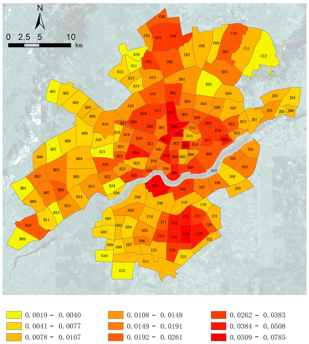
This study uses standard deviation model to assess the vitality level characteristics. It helps evaluate the degree of change in vitality. Low values signify little variation, and conversely, a high standard deviation suggests greater variability (Figure 3). Shenyang’s urban vitality exhibits the following spatial characteristics:
The distribution of urban vitality demonstrates a high degree of alignment with the spatial layout of urban master planning. High standard deviation values tend to be found along Qingnian Street and both banks of the Hunhe River, creating a distinctive “cross” spatial configuration. This phenomenon indirectly revealed the practical impact of the “One River, Two Banks” development strategy.
The identified high-vitality areas are predominantly concentrated around district economic centers. Regions displaying high deviation values are predominantly located in research units serving as commercial centers, cultural centers, transit hubs, business office complexes, industrial parks, and high-tech industrial parks.
Additionally, urban vitality exhibits a dynamic development momentum in newly developed urban districts. In Shenyang’s urban expansion, units showing significant progress in urban environmental conditions show high standard deviation values. This was maybe due to the outward growth of urban structures. New regions had been aggressively built, infrastructure had been consistently upgraded, functions had progressively diversified, and spatial quality had been continually improved. These changes drew the population to gather in the center of the city, consequently propelling the continuous improvement of urban vitality.

4.2. Built Environment Impact Factors

4.2.1. Factors Quantitative

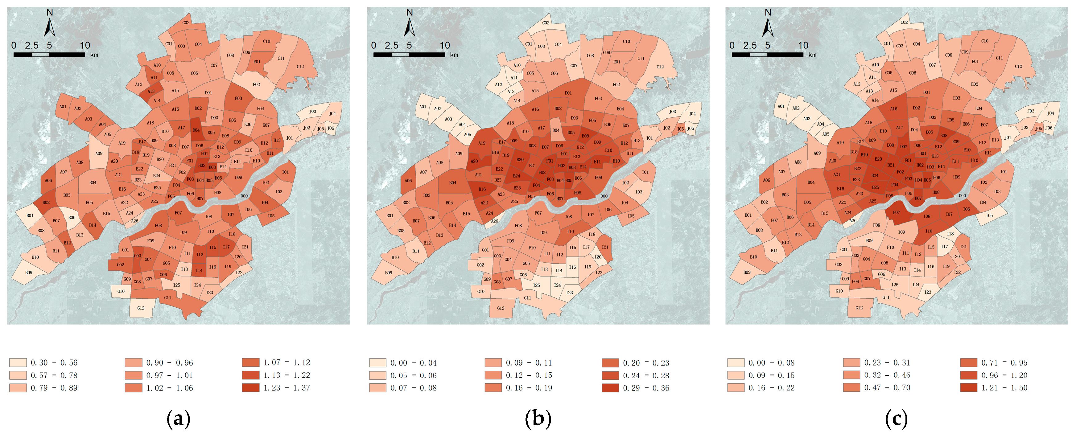
A quantitative system was developed for the urban built environment, which included five primary indicators: Land-use Mixed Degree, Development Intensity, Functional Facilities Supporting, Road Traffic Configuration, and Ecological Greening Environment, along with 14 secondary indicators (Figure 4).

4.2.2. Factors Collinearity Diagnosis

Before using MGWR, geographical variables were excluded, and then OLS was applied to evaluate collinearity among built environment factors.
The collinearity diagnosis revealed that X21 Building Density and X22 FAR exhibited collinearity problems under X2 Development Intensity. This may have been due to the fact that both factors were extracted from building outline data. FAR more effectively reflected development intensity than Building Density. Consequently, this study eliminated X21 Building Density while preserving X22 FAR. Other aspects had analogous procedures, which will not be detailed here. After adjusting (Table 4), the VIF values for all built environment factors were below 10, and the tolerance values were above 0.1, achieving the fundamental criteria for collinearity assessments, so enabling the establishment of OLS.

4.2.3. Coefficient of Factors Regression

We employed urban vitality as the dependent variable, with modified built environment factors employed as explanatory variables, to construct an OLS model. When Robust_Pr < 0.05, it signified a statistically significant association. In the regression results, the majority of the explanatory variables showed considerable significance (Table 5). R2 and Adjusted R2 represented the precision before and after adjustment, respectively. Both R2 and Adjusted R2 approximated 0.90, indicating that the regression model accounted for almost 90% of the results, proving a strong match.
The scatter plot showcases the relationship between the explanatory variables and the dependent variable. The direction of the slope indicates a positive or negative relationship. Only X52 vegetation coverage shows a negative connection with urban vitality. The correlations between the rest of the factors and urban vitality are positive. Regression analysis reveals that different built-environment factors have varying degrees of impact on urban vitality. X41 Bus Stop Density has consistently maintained the highest level. X33 Public Facility Density remains extremely stable. The regression coefficients of the other explanatory variables exhibit significant instability.

4.3. Spatial Heterogeneity

4.3.1. Spatial Auto-Correlation

The foundation for creating MGWR is that the variables show spatial auto-correlation; thus, the Moran’s I index is used to measure the spatial auto-correlation of influence mechanisms of built environment on urban vitality. The Moran I index ranges from −1 to 1, with higher absolute value representing a stronger spatial auto-correlation. The results indicate that the probability of influence mechanisms of built environment on urban vitality being randomly distributed in space is less than 1%. Influence mechanisms of built environment on urban vitality in space and exhibits spatial clustering characteristics. This suggests that influence mechanisms of built environment on urban vitality has spatial auto-correlation features, allowing to build an MGWR model (Table 6).

4.3.2. Multi-Scale Geographically Weighted Regression

In general, neither trend fitting nor average calculations will conceal essential geographical, social, and economic components. Since OLS treats the study area as a whole and neglects to consider spatial heterogeneity, further spatial regression analysis is needed. Comparing the results of MGWR and OLS (Table 7), it can be seen that the AICc of MGWR is significantly smaller than that of OLS. This indicates that MGWR performs better in terms of accuracy in data interpretation and future value prediction. R2 and Adjusted R2 are approximately 0.97, showing that MGWR can account for about 97% of the total data.
MGWR not only indicates the direction of the link between the dependent variable and explanatory variables but also demonstrates the degree of this effect by its absolute value. A positive coefficient suggests that the explanatory variable has a favorable effect on the dependent variable, with a bigger value denoting a stronger influence. A negative coefficient indicates that the explanatory variable has a limiting influence, with a bigger absolute value indicating a stronger restricting effect. MGWR analysis shows that the coefficient of the influence mechanisms of built environment on urban vitality fluctuates with location. Consequently, the correlation between the influence mechanisms of built environment on urban vitality and spatial dimensions is studied. The degree of influence can be measured by the MGWR correction coefficients (Table 8).

4.3.3. Regression Factor Results

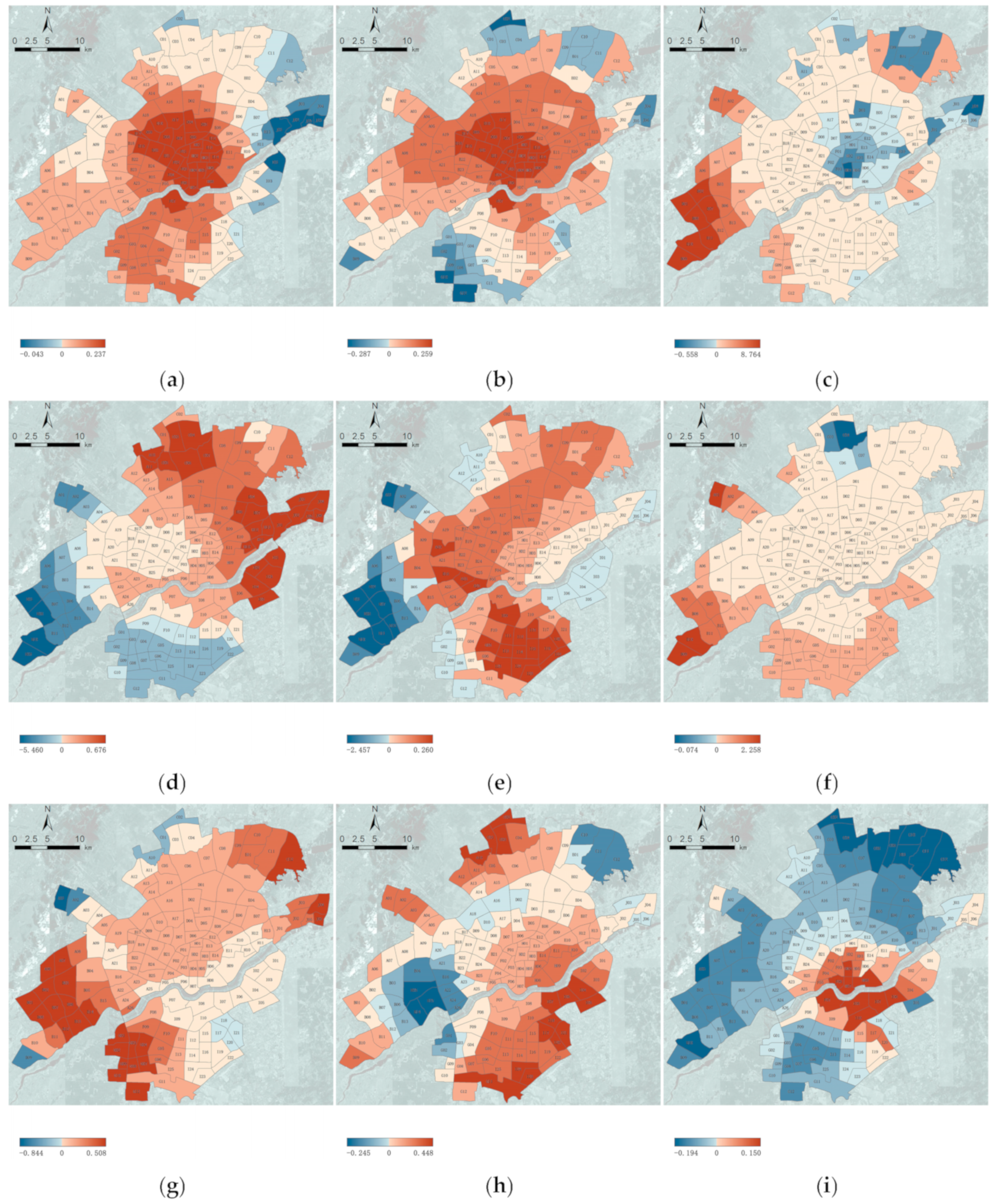
To clearly observe the spatial distribution, the regression coefficients for each unit were plotted on the map to explore how the built environment influences urban vitality. The value of “0” was established as the boundary for the built environment’s positive or negative influence on urban vitality. Warm colors were chosen to mark research units with positive coefficients and cool colors for those with negative coefficients. In positive units, the deeper the warm color, the more positive the impact of these explanatory variables on urban vitality. In negative regions, a deeper cool color correlated with a greater effect of these variables on urban vitality.
(1)
Land-use Mixed Degree
From the perspective of spatial distribution, the positively impacted area is centered around the urban core, showing a distribution pattern that gradually diminishes and spreads outward in concentric layers (Figure 5a). The coefficients in the eastern units generally exhibit negative values. The eastern region was far from the city center, maintaining excellent ecological resources, mainly serving as a natural scenic area and a villas residential community. X1 (Land-use Mixed Degree) was not the primary determinant influencing urban vitality in eastern region.
(2)
Development Intensity
The regression results of the X22 FAR show notable centripetal agglomeration characteristics in terms of geographical location (Figure 5b). The positive coefficients are predominantly located in the city center. As the distance from the central increases, the coefficients gradually decrease, demonstrating a significant decline.
(3)
Functional Facilities Supporting
The density of X31 Commercial Facilities, in contrast to other impacting factors, demonstrates a significantly diverse pattern (Figure 5c). An almost entirely negative correlation is observed in the research units located within the urban core area. This may have been due to a capacity limit for business facilities in that district. Exceeding the limit not only ceased to enhance urban vitality but may also have exerted a negative influence. Conversely, enhancing the density of commercial facilities in the urban peripheral regions might have substantially fostered the advancement in these places, serving as a beneficial driver for the district’s prosperity.
Regarding X33 (Public Facility Density), around 80% of the research units exhibit positive regression coefficients (Figure 5d). This notable phenomenon clearly showed that public facilities benefited the city’s overall vitality.
The differences concerning X35 (Leisure Facility Density) lie in the formation of multiple aggregation centers in spatial distribution (Figure 5e). Furthermore, these aggregation centers do not coincide with the city’s single center. When planning the layout of leisure facilities, greater emphasis should be placed on the spatial role of centers within each district rather than simply concentrating on an individual leisure center in the city.
(4)
Road Traffic Configuration
From X41 (Bus Stop Density) perspective, the positive research units count almost 90% of the total (Figure 5f). This notable phenomenon suggested that bus stops usually enhanced urban vitality. In the research area, there existed a single negatively related zone at the northern periphery. It was characterized by the new district center with a primary function of industry. The speedy development of infrastructure had not resulted in an enhancement of population vitality, indicating a negative correlation.
X42 (Subway Station Density) has a homogeneous beneficial effect (Figure 5g). The majority of the urban peripheral units demonstrated higher coefficient values, emphasizing the essential function of subway transportation in linking urban and suburban regions and promoting population mobility. In some rural and rarely inhabited regions, there was a necessity for economically feasible transportation alternatives, leading to a lowered demand for the subway.
Uniquely, not all regions experience enhanced urban vitality with the increase in X43 (Road Intersection density) (Figure 5h). In some study units where industry and manufacturing have a major presence, the increase in road density does not result in an improvement in urban vitality; rather, it presents adverse effects. The unique characteristics of industrial zones, including heavy freight transportation and industrial operations, contributed to increased traffic and noise pollution, which in turn blocked urban vitality.
(5)
Ecological Greening Environment
Concerning X52 (Vegetation Coverage), it shows a central positive correlation and a peripheral negative correlation trend (Figure 5i), similar to X11 (Functional Mixture Degree) and X22 (FAR). Interestingly, the center of X52 (Vegetation Coverage) slightly shifts to the south on the map, moving to the southern bank of the river. This phenomenon may have been attributed to the southern bank of the river being a newly built residential region, characterized by an enhanced living environment and ecological landscape. In comparison to the old city center, it possessed considerable ecological benefits, thereby resulting in the southerly shift of the concentration center.

5. Discussion

The spatial heterogeneity of MGWR-derived regression coefficients revealed that the impacts of various built environment determinants on urban vitality demonstrated significant spatial heterogeneity across observational units.

5.1. Land-Use Mixed Degree

The Land-use Mixed Degree exhibited a negative correlation in the ecological low-density areas of Shenyang, while demonstrating positive correlations in other regions. This study posited that for peripheral areas distant from the urban core, which maintain excellent ecological resources, increasing land-use mixture is not an effective means to enhance vitality. Conversely, excessive development may suppress vitality improvement to some extent. Tu (2020) indicated that not all functional mixtures contribute to vitality enhancement, as complex combinations could lead to functional disorder affecting urban vitality [43]. The experimental results of this study partially validate Tu’s perspective. This finding implies that in urban fringe ecological zones, enhancing Land-use Mixed Degree cannot be utilized as a strategy for urban vitality promotion.

5.2. Development Intensity

The Development Intensity in Shenyang presented a spatial pattern of positive correlation in the center and negative correlation in the periphery, with stronger central relevance. This study suggested that FAR effectively promotes vitality enhancement in urban centers, while inhibiting vitality improvement in fringe areas. This is attributed to the dense population aggregation in central areas requiring larger building spaces to accommodate activities, whereas low-density urban environments in peripheral regions contribute more significantly to vitality enhancement. Li et al. (2021) argued that high density satisfies diversified demands and facilitates human activities, though impacts vary across urban space types [46]. Xiao et al. (2021) noted nonlinear relationships between spatial morphology and urban vitality [50]. The experimental results partially validate these perspectives. This finding indicates that FAR’s impact on urban vitality exhibits spatial heterogeneity, necessitating context-specific FAR configurations to achieve vitality enhancement.

5.3. Functional Facilities Supporting

The three indicators under Functional Facilities Supporting (Commercial Facility Density, Public Facility Density, Leisure Facility Density) demonstrated distinct spatial characteristics in Shenyang. First, Commercial Facility Density showed negative correlation in the core area and weak correlations elsewhere, indicating commercial service facilities in urban centers have become redundant and constrain vitality enhancement. Second, Public Facility Density exhibited positive correlation in the northeast and negative correlation in the southwest, suggesting enhanced Public Facility Density promotes development in residential areas but has adverse effects in industrial zones. Third, Leisure Facility Density demonstrated significant positive correlation in Hunnan New Town (southern Shenyang) and weak/negative correlations elsewhere, reflecting urgent resident demand for leisure facilities in new urban areas. Li et al. (2021) emphasized differential impacts of POI types on vitality [46], while Lu et al. (2019) highlighted significant effects of POI combinations [49]. Wang et al. (2022) demonstrated that proximity to urban centers enhances regional vitality [51]. The experimental results partially validate these findings. This implies spatial heterogeneity in Functional Facilities’ impacts, with potential compound effects from facility combinations requiring holistic consideration.

5.4. Road Traffic Configuration

The two representative indicators under Road Traffic Configuration (Bus Stop Density and Subway Station Density) exhibited marked spatial disparities in Shenyang. Bus Stop Density showed negative correlation only in the northern emerging industrial district and positive correlations elsewhere, indicating rapid infrastructure development fails to enhance vitality in this area. Subway Station Density demonstrated significant positive correlation in rapidly developing fringe industrial zones and generally positive correlations citywide, likely due to job–housing imbalances where metro access mitigates traffic congestion impacts. Li et al. (2021) identified road width as critical for historic district revitalization [46], Yang (2021) emphasized metro accessibility impacts on Shenzhen’s vitality [47], and Xiao et al. (2021) linked street morphology (particularly traffic accessibility) to resident activity attraction [50]. Wang et al. (2022) highlighted destination accessibility’s role in regional connectivity and activity ranges [51]. The experimental results partially validate these perspectives. This finding underscores Road Traffic Configuration’s pivotal role in industrial city revitalization, particularly requiring emphasis on traffic factors in industrial area vitality studies.

5.5. Ecological Greening Environment

The Ecological Greening Environment in Shenyang demonstrated positive correlation in the center and negative correlation in peripheral areas. Notably, the “center” shifts southward to both banks of the Hun River rather than the geometric urban core, likely due to gentrification in Hunnan New District attracting residents with superior landscape quality. In contrast, Vegetation Coverage is not a vitality determinant in well-established old dist. Li et al. (2021) proposed that street greenery enhances vitality through ecological improvement, landscape beautification, and recreational space provision [46]. The experimental results partially validate this perspective. This finding suggests that urban vitality enhancement requires balancing demographic demands with built environment conditions.

6. Conclusions

This study took Shenyang as an example, introducing a methodology for built environment factors to thoroughly examine the influence mechanisms of urban vitality within certain planning units.
On one hand, the results corroborate that Shenyang’s vitality in the urban core area exhibits three main characteristics: policy-driven urban planning contributes significantly to boosting urban vitality; the agglomeration economy is a crucial factor influencing urban vitality; and the structural evolution is also an indispensable factor affecting urban vitality.
On the other hand, MGWR reveals three impacts: overall influences, location influences, and specific influences on the influence mechanisms in Shenyang’s central urban region.
(1)
Overall influences: Functional Mixture Degree, Bus Stop Density, and Subway Station Density all positively influenced the central urban area of Shenyang.
(2)
Location influences: FAR and Vegetation Coverage significantly enhanced the center area (exhibiting a diametrically opposite effect in peripheral area), whereas Commercial Facility Density and Road Density notably influenced the periphery region (exhibiting an opposite effect in center area).
(3)
Specific influences: Public Facility Density and Bus Stop Density exerted a substantial favorable influence on the industrial functional area.
There are two limitations in this study. Firstly, considering the spatial heterogeneity characteristics of the research object, this study adopts MGWR as the research method. The correlation between built environment and urban vitality is not a simple linear relationship, but there exist some non-equilibrium associations. In the future, improvements should be made in methodology to explore the trends and optimal thresholds. Secondly, this study only investigates an independent time period, ignoring the dynamic changes of many elements during the urban development process. In the future, it is planned to take the temporal dynamics into account.

Author Contributions

Conceptualization, X.L.; methodology, S.H.; software, S.H.; validation, W.X.; formal analysis, S.H.; investigation, S.H.; resources, W.X.; data curation, W.X.; writing—original draft preparation, S.H.; writing—review and editing, S.H.; visualization, Y.S.; supervision, X.L.; project administration, X.L.; funding acquisition, X.L. All authors have read and agreed to the published version of the manuscript.

Funding

This research received no external funding.

Conflicts of Interest

The authors W.X. are employed by Shenyang Urban Planning & Design Institute Co., Ltd. The remaining authors declare that the research was conducted in the absence of any commercial or financial relationships that could be construed as potential conflicts of interest.

References

  1. Caprotti, F.; Cowley, R.; Datta, A.; Broto, V.C.; Gao, E.; Georgeson, L.; Joss, S. The New Urban Agenda: Key Opportunities and Challenges for Policy and Practice. Urban Res. Pract. 2017, 10, 367–378. [Google Scholar] [CrossRef]
  2. National Bureau of Statistics. Statistical Bulletin of People’s Republic of China’s National Economic and Social Development in 2020; People’s Publishing House: Beijing, China, 2021.
  3. Zhang, Y.C.; Tu, T.Q.; Long, Y. Inferring Ghost Cities on the Globe in Newly Developed Urban Areas Based on Urban Vitality with Multi-Source Data. Habitat Int. 2025, 158, 103350. [Google Scholar] [CrossRef]
  4. Landry, C. Urban Vitality: A New Source of Urban Competitiveness; Archis Foundation: Amsterdam, The Netherlands, 2000; pp. 8–13. [Google Scholar]
  5. Pakoz, M.Z.; Isik, M. Rethinking Urban Density, Vitality and Healthy Environment in the Post-Pandemic City: The Case of Istanbul. Cities 2022, 124, 103598. [Google Scholar] [CrossRef]
  6. Tang, S.; Ta, N. How the Built Environment Affects the Spatiotemporal Pattern of Urban Vitality: A Comparison Among Different Urban Functional Areas. Comput. Urban Sci. 2022, 2, 39. [Google Scholar] [CrossRef] [PubMed]
  7. Jacobs, J. The Death and Life of Great American Cities; Random House: New York, NY, USA, 1961. [Google Scholar]
  8. Jiang, D.F. The Theory of City Form Vitality; Southeast University Press: Nanjing, China, 2007. [Google Scholar]
  9. Zhe, C.; Ma, S. Research on the Vitality of Urban Streets. Archit. J. 2009, S2, 121–126. [Google Scholar]
  10. Jiang, D.F.; Li, J.X. Several Thoughts About the Making of Vitality in Contemporary Cities. New Archit. 2016, 26, 21–25. [Google Scholar]
  11. Chen, Y.; Yu, B.; Shu, B.; Yang, L.; Wang, R. Exploring the Spatiotemporal Patterns and Correlates of Urban Vitality: Temporal and Spatial Heterogeneity. Sustain. Cities Soc. 2023, 91, 104440. [Google Scholar] [CrossRef]
  12. Doan, Q.C.; Ma, J.; Chen, S.; Zhang, X. Nonlinear and Threshold Effects of the Built Environment, Road Vehicles and Air Pollution on Urban Vitality. Landsc. Urban Plan. 2025, 253, 105204. [Google Scholar] [CrossRef]
  13. Li, X.; Li, Y.; Jia, T.; Zhou, L.; Hijazi, I.H. The Six Dimensions of Built Environment on Urban Vitality: Fusion Evidence from Multi-Source Data. Cities 2022, 121, 103482. [Google Scholar] [CrossRef]
  14. Boessen, A.; Hipp, J.R.; Butts, C.T.; Nagle, N.N.; Smith, E.J. The Built Environment, Spatial Scale, and Social Networks: Do Land Uses Matter for Personal Network Structure? Environ. Plan. B Urban Anal. City Sci. 2018, 45, 400–416. [Google Scholar] [CrossRef]
  15. Gong, H.; Wang, X.; Wang, Z.; Liu, Z.; Li, Q.; Zhang, Y. How Did the Built Environment Affect Urban Vibrancy? A Big Data Approach to Post-Disaster Revitalization Assessment. Int. J. Environ. Res. Public Health 2022, 19, 12178. [Google Scholar] [CrossRef]
  16. Jia, J.Y.; Song, J.F. Identifying the Relationship Between Urban Vitality and the “3D” Characteristics of Built Environment: A Case Study of Wuhan, China. Mod. Urban Res. 2020, 8, 59–66. [Google Scholar]
  17. Cao, Z.M.; Zhen, F.; Li, Z.X.; Lobsang, T. Urban Temporal Vibrancy Mode and Its Influencing Factors Based on Mobile Signaling Data: A Case Study of Nanjing, China. Hum. Geogr. 2022, 37, 109–117. [Google Scholar] [CrossRef]
  18. Sung, H.; Lee, S. Residential Built Environment and Walking Activity: Empirical Evidence of Jane Jacobs’ Urban Vitality. Transp. Res. Part D Transp. Environ. 2015, 41, 318–329. [Google Scholar] [CrossRef]
  19. Ta, N.; Zeng, Y.T.; Zhu, Q.Y.; Wu, J. Relationship Between Built Environment and Urban Vitality in Shanghai Downtown Area Based on Big Data. Sci. Geogr. Sin. 2020, 40, 60–68. [Google Scholar] [CrossRef]
  20. Yu, L.; Sheng, Y.H.; Liu, X.Y. A Method for Evaluating Urban Vitality Using the RAGA-PPM Model: A Case Study of Central Nanjing. J. Geo-Inf. Sci. 2024, 26, 2567–2582. [Google Scholar]
  21. Arbia, G. Spatial Econometrics: Statistical Foundations and Applications to Regional Convergence; Springer Science & Business Media: Berlin, Germany, 2006. [Google Scholar]
  22. Piketty, T.; Saez, E. Income Inequality in the United States, 1913–1998. Q. J. Econ. 2003, 118, 1–41. [Google Scholar] [CrossRef]
  23. Lee, S.; Kang, J.E. Impact of Particulate Matter and Urban Spatial Characteristics on Urban Vitality Using Spatiotemporal Big Data. Cities 2022, 131, 104030. [Google Scholar] [CrossRef]
  24. Mouratidis, K.; Poortinga, W. Built Environment, Urban Vitality and Social Cohesion: Do Vibrant Neighborhoods Foster Strong Communities? Landsc. Urban Plan. 2020, 204, 103951. [Google Scholar] [CrossRef]
  25. Chen, Y.; Yang, J.; Yu, W.; Ren, J.; Xiao, X.; Xia, J.C. Relationship Between Urban Spatial Form and Seasonal Land Surface Temperature Under Different Grid Scales. Sustain. Cities Soc. 2023, 89, 104374. [Google Scholar] [CrossRef]
  26. Yang, Y.; Wang, H.; Qin, S.; Li, X.; Zhu, Y.; Wang, Y. Analysis of Urban Vitality in Nanjing Based on a Plot Boundary-Based Neural Network Weighted Regression Model. ISPRS Int. J. Geo-Inf. 2022, 11, 624. [Google Scholar] [CrossRef]
  27. Zhang, A.; Li, W.; Wu, J.; Lin, J.; Chu, J.; Xia, C. How Can the Urban Landscape Affect Urban Vitality at the Street Block Level? A Case Study of 15 Metropolises in China. Environ. Plan. B Urban Anal. City Sci. 2021, 48, 1245–1262. [Google Scholar] [CrossRef]
  28. Zhang, A.; Li, W.; Wu, J.; Lin, J.; Chu, J.; Xia, C. Spatial Features of Urban Vitality and the Impact of Built Environment on Them Based on Multi-Source Data: A Case Study of Shenzhen. Trop. Geogr. 2021, 41, 1280–1291. [Google Scholar]
  29. Shi, Y.; Zheng, J.; Pei, X. Measurement Method and Influencing Mechanism of Urban Subdistrict Vitality in Shanghai Based on Multisource Data. Remote Sens. 2023, 15, 932. [Google Scholar] [CrossRef]
  30. Portugali, J. What Makes Cities Complex? In Complexity, Cognition, Urban Planning and Design; Portugali, J., Stolk, E., Eds.; Springer International Publishing: Cham, Switzerland, 2016; pp. 3–19. [Google Scholar] [CrossRef]
  31. Zhu, T.T.; Tu, W.; Le, Y.; Zhong, C.; Zhao, T.; Li, Q.; Li, Q. Sensing Urban Vibrancy Using Geo-Tagged Data. Acta Geod. Cartogr. Sin. 2020, 49, 365–374. [Google Scholar]
  32. Sun, H.H.; Jiang, Y.P. Spatial Heterogeneity of the Impact of Built Environment on Urban Vitality: A Case Study of the Central Urban Area of Nanjing. Geogr. Res. 2024, 43, 1700–1714. [Google Scholar]
  33. Wang, X.; Zhang, Y.; Yu, D.; Qi, J.; Li, S. Investigating the Spatiotemporal Pattern of Urban Vibrancy and Its Determinants: Spatial Big Data Analyses in Beijing, China. Land Use Policy 2022, 119, 106162. [Google Scholar] [CrossRef]
  34. Lynch, K. Good City Form; MIT Press: Cambridge, MA, USA, 1984. [Google Scholar]
  35. Gehl, J. Life Between Buildings: Using Public Space; Island Press: Washington, DC, USA, 2011. [Google Scholar]
  36. Tong, M. How Urban Fabric Can Help Sustain the Vitality of Cities. Urban Plan. Forum 2014, 21, 85–96. [Google Scholar]
  37. Jin, Y.J. Study on Urban Economic Vitality Index in China. Sci. Geogr. Sin. 2007, 27, 9–16. [Google Scholar]
  38. Della Spina, L. Multidimensional Assessment for “Culture-Led” and “Community-Driven” Urban Regeneration as Driver for Trigger Economic Vitality in Urban Historic Centers. Sustainability 2019, 11, 7237. [Google Scholar] [CrossRef]
  39. Wu, W.; Dang, Y.; Zhao, K.; Chen, Z.; Niu, X. Spatial Nonlinear Effects of Urban Vitality Under the Constraints of Development Intensity and Functional Diversity. Alex. Eng. J. 2023, 77, 645–656. [Google Scholar] [CrossRef]
  40. Wang, Z.; Wang, X.; Liu, Y.; Zhu, L. Identification of 71 Factors Influencing Urban Vitality and Examination of Their Spatial Dependence: A Comprehensive Validation Applying Multiple Machine-Learning Models. Sustain. Cities Soc. 2024, 108, 105491. [Google Scholar] [CrossRef]
  41. Kim, Y.L. Seoul’s Wi-Fi Hotspots: Wi-Fi Access Points as an Indicator of Urban Vitality. Comput. Environ. Urban Syst. 2018, 72, 13–24. [Google Scholar] [CrossRef]
  42. Meng, Y.; Xing, H. Exploring the Relationship Between Landscape Characteristics and Urban Vibrancy: A Case Study Using Morphology and Review Data. Cities 2019, 95, 102389. [Google Scholar] [CrossRef]
  43. Tu, W.; Zhu, T.; Xia, J.; Zhou, Y.; Lai, Y.; Jiang, J.; Li, Q. Portraying the Spatial Dynamics of Urban Vibrancy Using Multisource Urban Big Data. Comput. Environ. Urban Syst. 2020, 80, 101428. [Google Scholar] [CrossRef]
  44. Guo, J.; Wang, J.; Xu, C.; Song, Y. Modeling of spatial stratified heterogeneity. GISci. Remote Sens. 2022, 59, 1660–1677. [Google Scholar] [CrossRef]
  45. Yue, Y.; Zhuang, Y.; Yeh, A.G.O.; Xie, J.-Y.; Ma, C.-L.; Li, Q.-Q. Measurements of POI-Based Mixed Use and Their Relationships with Neighbourhood Vibrancy. Int. J. Geogr. Inf. Sci. 2017, 31, 658–675. [Google Scholar] [CrossRef]
  46. Li, M.; Liu, J.; Lin, Y.; Xiao, L.; Zhou, J. Revitalizing Historic Districts: Identifying Built Environment Predictors for Street Vibrancy Based on Urban Sensor Data. Cities 2021, 117, 103305. [Google Scholar] [CrossRef]
  47. Yang, J.; Cao, J.; Zhou, Y. Elaborating Non-Linear Associations and Synergies of Subway Access and Land Uses with Urban Vitality in Shenzhen. Transp. Res. Part A Policy Pract. 2021, 144, 74–88. [Google Scholar] [CrossRef]
  48. Chen, T.; Hui, E.C.M.; Wu, J.; Lang, W.; Li, X. Identifying Urban Spatial Structure and Urban Vibrancy in Highly Dense Cities Using Georeferenced Social Media Data. Habitat Int. 2019, 89, 102005. [Google Scholar] [CrossRef]
  49. Lu, S.; Huang, Y.; Shi, C.; Yang, X. Exploring the Associations Between Urban Form and Neighbourhood Vibrancy: A Case Study of Chengdu, China. ISPRS Int. J. Geo-Inf. 2019, 8, 165. [Google Scholar] [CrossRef]
  50. Xiao, L.; Lo, S.; Liu, J.; Zhou, J.; Li, Q. Nonlinear and Synergistic Effects of TOD on Urban Vibrancy: Applying Local Explanations for Gradient Boosting Decision Tree. Sustain. Cities Soc. 2021, 72, 103063. [Google Scholar] [CrossRef]
  51. Wang, B.; Lei, Y.; Xue, D.; Liu, J.; Wei, C. Elaborating Spatiotemporal Associations Between the Built Environment and Urban Vibrancy: A Case of Guangzhou City, China. Chin. Geogr. Sci. 2022, 32, 480–492. [Google Scholar] [CrossRef]
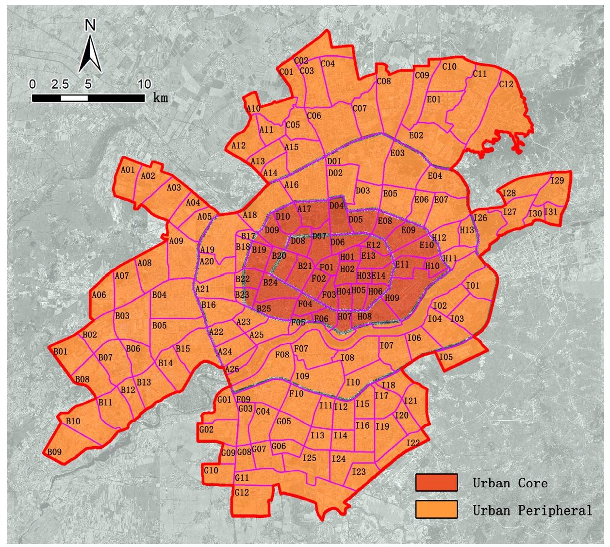
Figure 1. Study scope map.
Buildings 15 02989 g001
Figure 2. Data processing diagram. (a) Population density—Raster Clipping. (b) Population density—Feature to Polygon. (c) Population density—Create Fishnet. (d) Population density—Join Data Spatially.
Buildings 15 02989 g002
Figure 3. Spatial distribution map of standard deviation of urban vitality.
Buildings 15 02989 g003
Figure 4. Built environment factors distribution map. (a) Functional Mixture Degree. (b) Building Density. (c) FAR. (d) Commercial Facility Density. (e) Business Facility Density. (f) Public Facility Density. (g) Living Facility Density. (h) Leisure Facility Density. (i) Bus Stop Density. (j) Subway Station Density. (k) Road Density. (l) Road Intersection Density. (m) Park Square Density. (n) Vegetation Coverage.
Buildings 15 02989 g004aBuildings 15 02989 g004b
Figure 5. Factor Regression Distribution Diagram. (a) Functional Mixture Degree. (b) FAR. (c) Commercial Facility Density. (d) Public Facility Density. (e) Leisure Facility Density. (f) Bus Stop Density. (g) Subway Station Density. (h) Road Density. (i) Vegetation Coverage.
Buildings 15 02989 g005
Table 1. Data source table.
Name of DataSource of DataRemarks
Spatial Distribution Data on Population DensityOak Ridge National Laboratory (ORNL)The spatial resolution is 1 km.
Night Light DataNational Oceantic and Atmospheric AdministrationThis study used DMSP/OLS and NPP/VIIRS Night Light Data
GDP Kilometric Grid DataGeographical Information Monitoring Cloud PlatformUtilizing diverse spatial data, including height and topography, it produces 1 km × 1 km GDP raster data for each industry
POI dataamapData encompassing 23 primary categories, numerous secondary categories, and myriad tertiary categories.
Building DataamapThe data includes raster boundaries of building outlooks and height features
Road DataOpen street mapThe data includes details regarding road location, layout, and length.
Normalized Difference Vegetation IndexNASAThe spatial resolution of the data is 250 m.
Table 2. Factor quantization table.
ItemWeights
Social VitalityDegree of population agglomeration 0.2258
Intensity of spatial interaction between residents and the urban environment 0.217
Economic Vitality Spatial distribution of GDP 0.317
Cultural VitalityDistribution of cultural facilities0.2402
Table 4. Statistical table of collinearity test for built environment factors.
Primary IndicatorSecondary IndicatorBefore TestAfter Test
CodeNameCodeNameVIF ValueToleranceVIF ValueTolerance
X1Land-use Mixed DegreeX11Functional Mixture Degree1.3630.7331.2760.783
X2Development IntensityX21Building Density10.0120.1----
X22FAR12.0440.0833.6250.276
X3Functional Facilities SupportingX31Commercial Facility Density17.7350.0568.4240.119
X32Business Facility Density3.7860.264----
X33Public Facility Density10.4370.0966.3370.158
X34Living Facility Density26.3160.038----
X35Leisure Facility Density20.7450.0489.160.109
X4Road Traffic ConfigurationX41Bus Stop Density7.6980.136.2640.16
X42Subway Station Density4.1230.2433.310.302
X43Road Density18.0230.0554.9910.2
X44Road Intersection Density23.8250.042----
X5Ecological Greening EnvironmentX51Park Square Density1.7140.584----
X52Vegetation Coverage4.6880.2133.8930.257
Table 5. Statistical table of OLS results for urban vitality.
X11X22X31X33X35X41X42X43X52
Functional Mixture DegreeFARCommercial Facility DensityPublic Facility DensityLeisure Facility DensityBus Stop DensitySubway Station DensityRoad Intersection DensityVegetation Coverage
Robust_Pr0.0482 *0.0000 *0.3365 0.0052 *0.0759 0.0000 *0.0302 *0.0342 *0.6934
Coefficient0.08480.1789 −0.0798 0.1705 0.1210 0.2802 0.0854 0.1275 0.0228
Buildings 15 02989 i001Buildings 15 02989 i002Buildings 15 02989 i003Buildings 15 02989 i004Buildings 15 02989 i005Buildings 15 02989 i006Buildings 15 02989 i007Buildings 15 02989 i008Buildings 15 02989 i009
Note: R2 = 0.900181, Adjust R2 = 0.893898, AICc = −394.477622. * indicates that the coefficient is statistically significant (p < 0.01).
Table 6. Statistical table of spatial auto-correlation test results.
Moran IZ Valuep Value
0.601134.99720.0000
Table 7. Table of comparison between OLS and MGWR.
FactorsMGWR ResultsOLS Results
AICc−1384.51−394.477622
R20.9702550.900181
Adjust R20.9696630.893898
Table 8. Table of MGWR correction coefficients.
Explanation VariablesMeanMinimumLower Quartile MedianUpper QuartileMaximum
CODENAME
X11Functional Mixture Degree0.098−0.0510.040.0840.1480.355
X22FAR0.049−0.431−0.0340.0730.1430.372
X31Commercial facility density0.364−3.437−0.0510.1040.4068.764
X33Public facility density0.079−5.460.060.1880.3441.462
X35Leisure facility density−0.079−6.905−0.0410.0540.1160.496
X41Bus stop density0.258−0.8060.1640.2340.3092.258
X42Subway station density0.135−0.8440.0580.0930.1781.542
X43Road Intersection density0.122−0.2450.0420.1090.1990.755
X52Vegetation coverage−0.067−0.283−0.121−0.072−0.0080.156
Disclaimer/Publisher’s Note: The statements, opinions and data contained in all publications are solely those of the individual author(s) and contributor(s) and not of MDPI and/or the editor(s). MDPI and/or the editor(s) disclaim responsibility for any injury to people or property resulting from any ideas, methods, instructions or products referred to in the content.