Article

Revealing Nonlinear and Spatial Interaction Effects of Built Environment on Ride-Hailing Demand in Nanjing, China

1
College of Automobile and Traffic Engineering, Nanjing Forestry University, Nanjing 210037, China
2
College of Civil and Transportation Engineering, Hohai University, Nanjing 210098, China
*
Authors to whom correspondence should be addressed.
Buildings 2025, 15(16), 2967; https://doi.org/10.3390/buildings15162967
Submission received: 25 June 2025 / Revised: 30 July 2025 / Accepted: 11 August 2025 / Published: 21 August 2025
(This article belongs to the Section Building Energy, Physics, Environment, and Systems)

Abstract

Numerous machine learning models are viewed as an important means for evaluating the built environment (BE) features and travel behavior. However, most of them ignore the interaction effects of the BE and geographic locations. To strengthen their spatial interpretability, the study combines the random forest and GeoShapley method to scrutinize the nonlinear and spatial interaction effects of the BE features on ride-hailing demand using multi-source data from Nanjing, China. The results indicate that the land use mixture, the interaction between the distance to city center and geographic locations, and geographic locations are the most essential factors influencing ride-hailing demand. All BE features exhibit nonlinear effects on ride-hailing demand. Moreover, Among the BE features, distance to city center, land use mixture, and distance to metro stop demonstrate significant interaction effects with geographic locations. The findings indicate the necessity of incorporating geospatial analysis into the relationships and offer implications for implementing location-specific strategies.

1. Introduction

Because of their flexibility and convenience, ride-hailing services have become an essential component of the urban transportation system [1]. For example, as a main sharing economy market, China has more than 400 million ride-hailing users as of 2024. On the one hand, urban planners are seeking to address existing mobility disparities and enhance multimodal accessibility in regions underserved by public transportation systems. Conversely, the proliferation of ride-hailing services often causes concerns regarding traffic congestion and safety. Hence, numerous studies have scrutinized the contributors to ride-hailing demand [2,3], among which the built environment (BE) usually plays an important role.
Although the literature has examined the connection between the BE and ride-hailing demand, two main research gaps remain. First, because transportation network companies tend to be unwilling to share their data [4], prior studies have mainly analyzed data of a certain transportation network company. However, the data from one certain company may not reflect the demand of the overall population. In particular, the connection between the BE and ride-hailing demand remains inconclusive in the literature [1,5]. This inconsistent phenomenon may be partially explained by the fact that different pricing strategies of transportation network companies may make them attract different groups and primarily serve in different areas [6]. In this regard, the above limitation may cause biased estimations and inappropriate policy recommendations. Second, prior studies have applied machine learning methods combined with the Shapley additive explanation (SHAP) to scrutinize the nonlinear connections of the BE with ride-hailing demand [7,8]. Although SHAP strengthens the interpretability of machine learning methods, it cannot accommodate the spatial effects within a unified framework [9,10]. This omission of the spatially varying effects of the BE features may weaken the effectiveness of planning strategies. However, it is unclear whether and how the BE has spatial interaction effects on ride-hailing demand. Moreover, traditional spatial models, such as Geographically Weighted Regression (GWR), are typically based on linear assumptions, which limit their ability to capture the potential nonlinear relationships between BE features and ride-hailing demand. As a result, they may overlook threshold effects and complex interactions that are commonly observed in real-world urban systems.
To address the limitations, the research scrutinizes the spatial interaction effects of the BE features on ride-hailing demand by integrating the random forest (RF) model with the GeoShapley method. It contributes to the literature in the following ways: (1) it explores ride-hailing order data of all transportation network platforms within an entire city. Such a dataset not only better reflects the distribution of ride-hailing demand but also makes the study the first to explore its connection with the BE features from the perspective of the overall demand; (2) it scrutinizes the interaction effects of the BE and geographic locations on ride-hailing demand based on the GeoShapley method, which is a spatially explicit adaptation of the SHAP paradigm. The nonlinear effects of the BE features are also revealed within the unified framework. The findings not only deepen our understanding of their connections but also offer insights for promoting location-specific strategies.

2. Literature Review

2.1. BE and Ride-Hailing Demand

The BE refers to the man-made surroundings that support human activities, often measured by the “5Ds” framework, i.e., density, design, diversity, destination accessibility, and distance to transit [11,12,13]. Due to its long-term effect on urban transport, the BE and its interaction with travel behavior have received extensive research interest [14,15,16,17,18].
As a crucial element of urban transportation, ride-hailing and its connection with the BE have been extensively investigated within the “5Ds” framework [19,20,21]. For example, Wang and Noland analyzed the link of ride-hailing demand with spatial characteristics in Chengdu, China, finding a significant positive correlation between ride-hailing demand and population density (PD) as well as road density. Additionally, there exists significant spatial heterogeneity in the effect of PD [22]. This aligns with findings from Sabouri et al.’s and Ghaffar et al.’s studies [5,23]. In terms of diversity, the relationship of land use mixture (LUM) with ride-hailing demand has not reached a consensus across different regions. A negative connection between the two issues is observed in Chengdu, where residents in areas with higher LUM tend to prefer walking or biking to reach their destinations [22]. Conversely, in Texas, USA, studies show that ride-hailing demand increases significantly with LUM [24]. These differences highlight the critical role of land use characteristics in shaping travel demand. In areas with high functional integration, residents’ daily activities are more concentrated, enabling travel needs to be met through walking or biking. Meanwhile, in some regions or city centers, the diversity of demand, combined with the limitations of public transit, results in high ride-hailing demand. In addition, Sabouri et al. observed that Uber demand shows positive connections with proximity to transit stops but is negatively linked to intersection density and destination accessibility [23]. Li et al. employed a GWR model to investigate the influential variables across different periods and trip distances. Their findings reveal significant spatial and temporal heterogeneity in the influence of bus stops [25].
In addition to the aforementioned BE features, studies have confirmed that demographic factors and demand management strategies also play a role in affecting ride-hailing demand. From a demographic perspective, research has found that individuals with higher education levels and residing in areas with higher housing price (HP) prefer ride-hailing services [5,26]. Siddiq and Taylor further examined the influence of gender on ride-hailing usage in the Los Angeles area, revealing that women use ride-hailing services more frequently than men for family-related trips [27]. Moreover, Gomez et al. [28] identified that environmental awareness significantly affects ride-hailing usage in Madrid, Spain, whereas this effect is less pronounced in American cities. Individuals with higher environmental awareness tend to reduce their utilization of ride-hailing services. From a demand management perspective, studies have shown that factors, such as limited parking availability, high parking fees, travel distance, and travel time, can significantly influence ride-hailing demand [5,29].

2.2. Related Models

Various models have been employed in the literature, such as regression models and machine learning models. For instance, several types of regression models are frequently employed to identify key factors influencing ride-hailing demand [30]. Yet, these approaches cannot capture the spatial heterogeneity in their connections. To address this limitation, researchers have incorporated spatial econometric models into studies on their relationships [31,32,33,34,35,36]. Cao et al. [35] constructed a multiscale geographically weighted regression (MGWR) model using ride-hailing trip data across different periods to analyze the spatiotemporal heterogeneity of the BE’s impact on ride-hailing demand. Their findings show that during peak hours, PD and HP significantly affect ride-hailing demand, while commercial and residential land uses exhibit significant spatial heterogeneity. The MGWR model also demonstrates better performance compared to the ordinary least squares regression.
In recent years, machine learning approaches have been increasingly applied to ride-hailing research due to their powerful learning capabilities and adaptability to complex nonlinear relationships [33,34,35,36,37,38,39]. Differing from conventional regression models based on linear assumptions, machine learning approaches can uncover potential nonlinear relationships between the BE and travel behavior. For example, Li et al. [40] used urban data from Haikou to construct gradient boosting trees to scrutinize their potential relationships. The results show that the top three most influential variables are restaurant density, educational institution density, and distance to city center (DCC). Additionally, some studies have focused on the interactions among variables, further enriching the understanding of their combined effects [41,42]. However, while machine learning models overcome the limitations of linear assumptions, they typically cannot capture the interactions among spatial units.
In sum, although the literature has offered evidence on the BE and ride-hailing demand, most of them use data from a certain transportation network company. Moreover, it is largely unknown whether the BE has spatial interaction effects on ride-hailing. To address these limitations, this study attempts to integrate an RF approach with the GeoShapley method to capture both nonlinear and spatial interaction effects of the BE on ride-hailing demand using order data from all transportation network companies in Nanjing.

3. Methodology

3.1. Study Region and Ride-Hailing Demand

Nanjing is a key central city and comprehensive transportation hub in eastern China, covering 6587.04 square kilometers across 11 administrative districts. With its high PD, developed transportation system, and supportive urban policies, Nanjing provides a typical urban context for examining the spatial and nonlinear impacts of the BE on ride-hailing demand. This study concentrates on Nanjing’s central urban areas, a hotspot for ride-hailing trips, as the study region. The study region includes Xuanwu, Gulou, Jianye, Qinhuai, Qixia, and Yuhuatai districts (Figure 1). To capture the effect of the BE on ride-hailing demand, the study region is divided into 500 m × 500 m grids [43]. After excluding grids with zero ride-hailing demand and areas without human activity (e.g., water bodies and mountain peaks), a total of 1677 grids are obtained for the analysis.
The ride-hailing demand is sourced from the official platform of the Nanjing Municipal Transportation Bureau, encompassing order data from all 10 transportation network companies. Given variations in user composition, market share, and spatial distribution across platforms, this study integrates all of the aforementioned transportation network companies’ data to reduce bias and improve the accuracy and robustness of the analysis of the link between BE features and ride-hailing demand. The order data on a typical workday (20 April 2022) are used for this analysis. The dataset includes various attributes, such as the pick-up and drop-off coordinates, the times passengers board and alight, and total trip mileage. After error-checking and clearing the data, a total of 116,475 valid ride-hailing records are retained in the study region.

3.2. Independent Variable

The study considers the effects of the BE and demographic features. The BE features are measured based on the “5Ds” framework [44,45]. Related data are sourced from the LandScan Global Population Database, AMAP, and OpenStreetMap. Population size within each grid is used to represent the dimension of density, while road length (RL) and DCC are selected to represent design and destination accessibility. The dimension of distance to transit is characterized by four variables: bus stop density (BSD), metro stop density (MSD), distance to metro station (DMS), and distance to bus stop (DBS). Diversity is captured through LUM, derived from seven categories of points of interest (POIs) provided by AMAP, including restaurant facilities, business establishments, education and culture facilities, tourist attractions, residential and commercial areas, recreation and entertainment facilities, and healthcare facilities. LUM is assessed through the entropy index [46], calculated as follows:
E j = A j p ln A j p ln P j
where E j represents the mixed entropy index of grid j. A j p denotes the proportion of the p t h type of POI in grid j. P j indicates the number of POI categories in grid j.
We consider HP to be a demographic factor in the study. The data are crawled from LIANJIA, one of the largest real estate platforms in China. The average HP within each grid is calculated based on the data from various residential communities. For grids with missing HP data, the Empirical Bayesian Kriging method is used for interpolation to estimate the variable values at unknown locations [47]. Geographic locations are represented by UTM_X and UTM_Y, which correspond to the longitude and latitude of the grid centroid point. The specific descriptive statistics of variables are shown in Table 1.

3.3. Methods

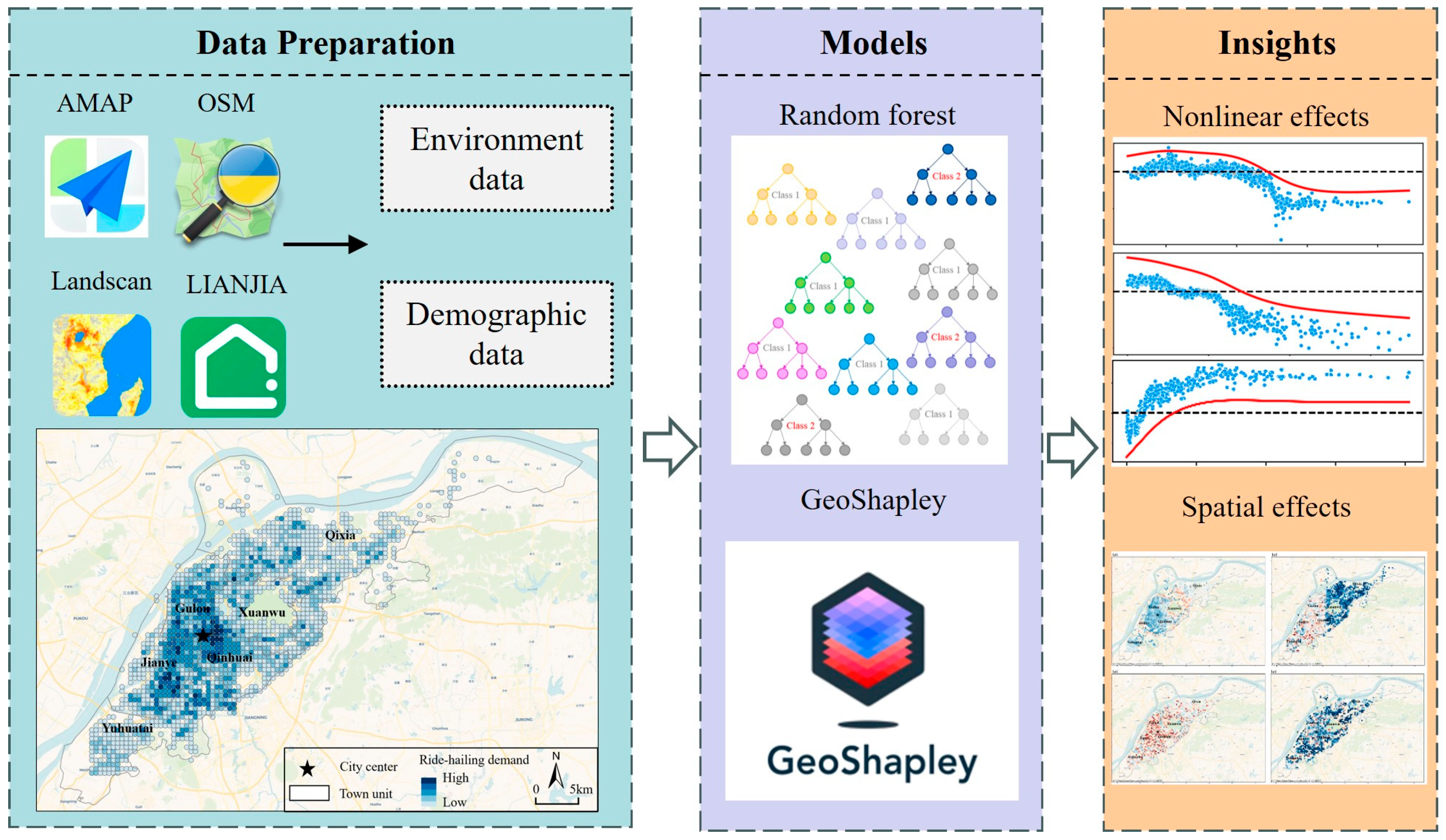
This study follows the research framework illustrated in Figure 2 and consists of three main stages. The data preparation involves the collection of BE, demographic, and ride-hailing data. In the model construction stage, RF and GeoShapley method are employed to develop predictive models. Finally, the result analysis stage examines the nonlinear effects of BE variables on ride-hailing demand, as well as their spatial interaction dynamics.

3.3.1. RF Model

RF is a typical ensemble learning algorithm. It learns each decision tree using bootstrapped random sampling with replacement, generates predictions based on the continuous outputs of each tree, and integrates the final result by averaging or weighted average. Compared to other machine learning models, RF is well-suited for high-dimensional datasets, offering both high robustness and interpretability. The model can effectively uncover the nonlinear relationships between variables, and, thus, it has been widely used in transport planning [48,49]. In the study, the ride-hailing demand in a log format is the dependent variable. BE features and geographic locations are treated as independent variables. The RF model is constructed as follows:
y ^ ( x ) = 1 N n = 1 N y ( x ; θ n )
where y ^ ( x ) represents the final predicted value of the response. N refers to the number of decision trees. y ( x ; θ n ) denotes the predicted values of the independent variables in the n t h tree. θ n represents the random variables that are independent and identically distributed.

3.3.2. GeoShapley Method

RF demonstrates superior predictive performance but struggles to intuitively explain the specific contributions of independent variables and their spatial effects. To address this, the GeoShapley method, a spatially explicit adaptation of the SHAP paradigm, is introduced to incorporate geographic longitude and latitude as joint features for the analysis.
The traditional Shapley value assumes that features are independent of each other and quantifies each feature’s contribution to the response. The contribution of each feature is calculated as the weighted average of all marginal contributions as follows:
φ j = S M \ j s ! ( p s 1 ) ! p ! ( f ( S j ) f ( S ) )
where φ j is the contribution of variable j to the response. p represents the set of all variables. s denotes a subset of variables. M \ j refers to the set obtained by removing variables j from M . f ( S j ) indicates the predicted response after adding variable j . f ( S ) represents the prediction result based solely on subset s .
GeoShapley, based on the SHAP framework from game theory, extends machine learning models to incorporate geospatial data. It integrates geographic coordinates as joint features into model predictions, enabling the quantification and interpretation of spatial effects within machine learning models. Furthermore, it analyzes the linear or nonlinear effects of the BE features as non-spatial features. GeoShapley decomposes complex prediction outcomes into the contributions of spatial effects, non-spatial feature effects, and the interaction between geographic locations and non-spatial factors, thereby uncovering the underlying mechanisms of black-box models [50]. The mathematical expression for the GeoShapley value is as follows:
y ^ = ϕ 0 + ϕ G E O + j = 1 p ϕ j + j = 1 p ϕ ( G E O , j )
where y ^ represents the estimated ride-hailing demand. ϕ 0 denotes the average predicted value across all samples, serving as the global intercept. ϕ G E O is the marginal contribution of geographic locations (longitude and latitude) to the prediction results, which is used to measure spatial effects within the model. p denotes the total count of non-location features in the model. ϕ j represents the contribution of a non-spatial feature j to the prediction results, which quantifies the global linear or nonlinear spatial effects of non-spatial features. ϕ ( G E O , j ) indicates the contribution of the interaction between geographic locations and each non-spatial feature j to the prediction results, which is used to measure the spatial effects of individual features. The expressions for ϕ G E O , ϕ j and ϕ ( G E O , j ) are as follows:
ϕ G E O = S M \ \ { G E O } s ! ( p s g ) ! ( p g + 1 ) ! ( f ( S { G E O } ) f ( S ) )
ϕ j = S M \ \ { j } s ! ( p s g ) ! ( p g + 1 ) ! ( f ( S { j } ) f ( S ) )
ϕ ( G E O , j ) = S M \ \ { G E O , j } s ! ( p s g 1 ) ! ( p g + 1 ) ! Δ { G E O , j }
Δ { G E O , j } = f ( S { G E O , j } ) f ( S { G E O } ) f ( S { j } ) + f ( S )
where G E O represents a set of geographical locations defined by geographic coordinates (longitude and latitude), with g taking a value of 2 in this study. The set p includes all features, encompassing both geographical locations and non-spatial features. The variable j denotes an individual non-spatial feature, while s represents a subset of features. The notations M \ \ j , M \ \ G E O and M \ \ G E O , j refer to subsets of p with specific exclusions, i.e., excluding the non-spatial feature j , excluding all geographical features, and excluding both geographical features and the non-spatial feature j , respectively. The function f ( S ) indicates the model’s prediction based on the subset s while f ( S j ) and f ( S G E O ) represent the predictions when the subset s is expanded to include the non-spatial feature j or all geographical features, respectively. Finally, the interaction term Δ G E O , j quantifies the contribution of the interaction effect between geographical and non-spatial feature j to the model’s prediction.
To capture the interaction effects of the BE and geographic locations, a spatially varying parameter is calculated in the GeoShapley method. Similarly to the regression coefficients in GWR models, the parameter can reflect the spatial distribution pattern and neighborhood variations in the interaction effects. The parameter can be represented as follows:
β j = ϕ j + ϕ ( G E O , j ) x j E ( x j )
where β j represents the spatially varying parameter. x j represents the actual value of feature j in the sample. E ( x j ) denotes the mean value of feature j .

4. Results

4.1. Collinearity Test and Model Performance

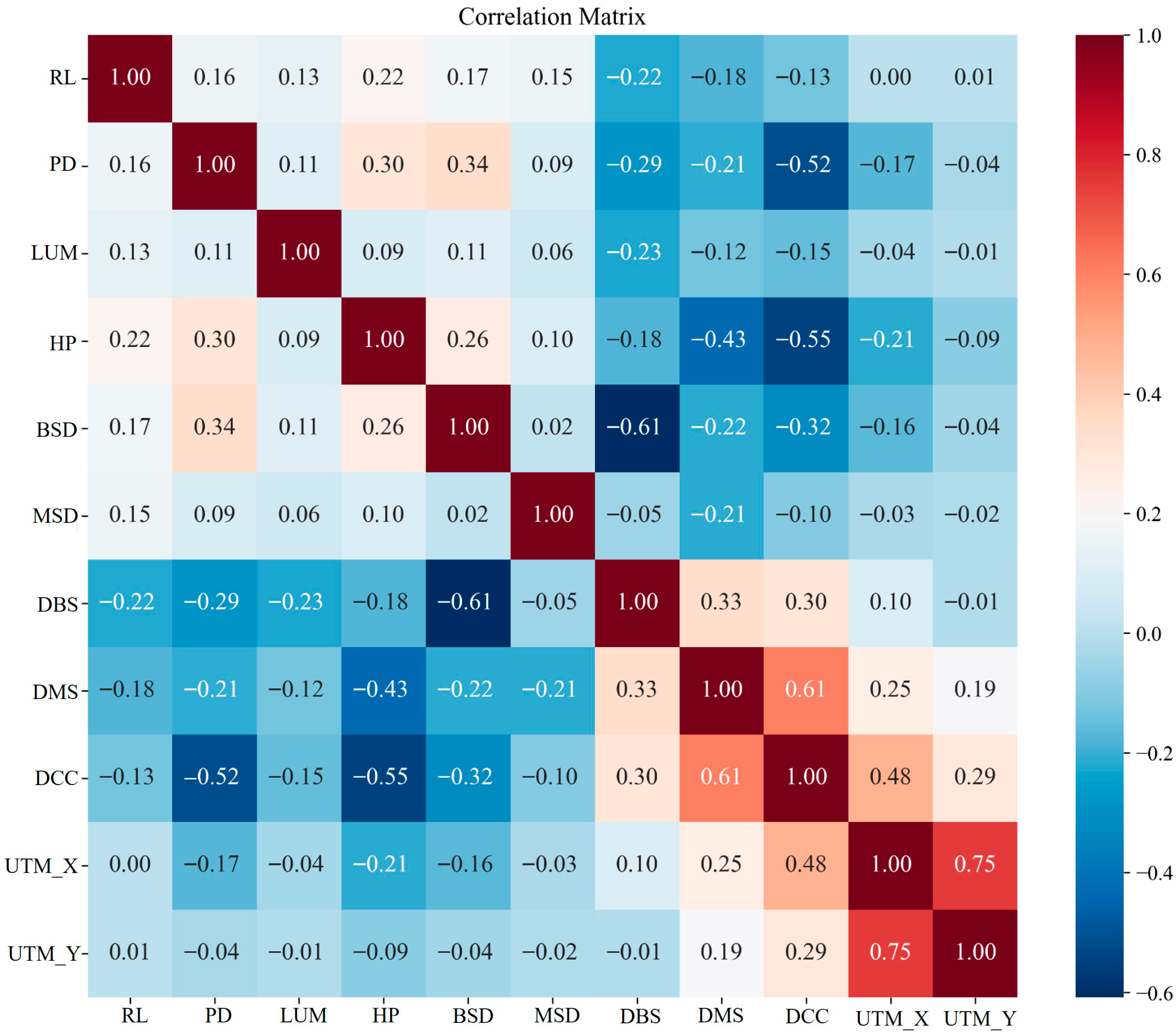
To ensure the stability and reliability of estimated results, a collinearity test for all independent variables is conducted. Figure 3 presents the estimated correlation coefficients of the variables. Except for the longitude and latitude, the correlation coefficients of other variables display relatively low correlations [50]. The significant correlation between the longitude and latitude is reasonable because the study region is divided into 500 m × 500 m grids.
To further validate the fitting performance, two benchmark models were constructed for comparison, including an extreme gradient boosting tree (XGBoost) model and a GWR model. The performance of the three models is summarized in Table 2. The RF model demonstrates better performance according to the estimations, compared to the XGBoost and GWR models. Therefore, the results of the RF model are presented and analyzed in the following sections.

4.2. Importance and Nonlinear Effects

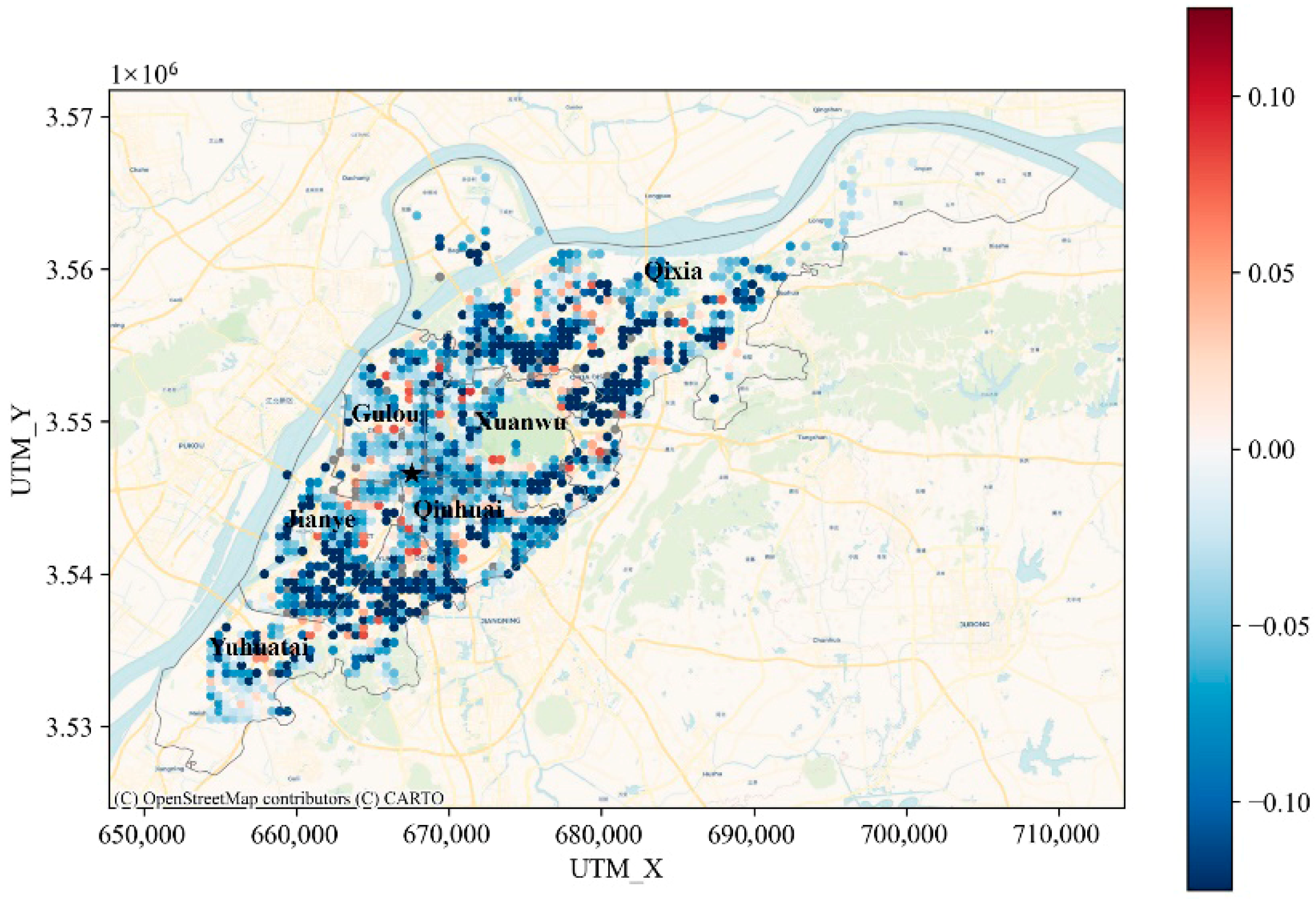
The summary statistics for the GeoShapley values can be found in Appendix A. Figure 4 presents the effects of the BE, geographic locations, and their interactions on ride-hailing demand. In the figure, GEO is the geographic location, which is represented by the combined x and y coordinates. Its interaction with one specific BE feature is represented by the BE feature × GEO. The three types of features are ranked from highest importance to lowest importance. Among the features, LUM ranks first in terms of importance, indicating that LUM is the most influential factor. Specifically, LUM features with larger values are concentrated in the positive range of the GeoShapley values, while samples with smaller feature values are concentrated in the negative range, indicating a positive relationship between the two issues. The interaction between the DCC and geographic locations ranks second in explaining ride-hailing demand. The interaction is primarily distributed in the positive range of the GeoShapley values. The effect of geographic locations on ride-hailing demand varies, indicating that differences in demand are shaped by the varying locational conditions across the city. DCC exhibits a negative effect on ride-hailing demand, with its contribution less significant than the interaction between DCC and geographic locations. In contrast, the interactions between the other BE features and geographic locations show relatively lower importance than corresponding BE features. DMS and HP exhibit negative effects on ride-hailing demand. RL and PD demonstrate a positive relationship with the response, indicating that areas with better road connectivity and higher population densities attract more ride-hailing trips, consistent with previous studies [23]. The effects of BSD and MSD are relatively weak.
Figure 5 visualizes the nonlinear effects of the BE and demographic features on ride-hailing demand by providing the marginal contribution of each feature to ride-hailing demand while holding other features constant. The figure shows that most BE factors exhibit nonlinear effects on ride-hailing demand, with varying effective ranges and threshold effects. RL and PD both follow a trend of initially increasing and then stabilizing. RL exhibits a threshold effect of around 2 km, indicating that ride-hailing platforms need to consider RL when scheduling services. Beyond this threshold, ride-hailing demand levels decrease as RL increases. PD influences ride-hailing demand significantly up to a threshold of 15,000 persons, after which the effect becomes minimal, suggesting that beyond a certain level, the impact of PD on demand is limited. LUM first increases, then decreases, with a positive correlation to ride-hailing demand between 0.3 and 0.8. However, beyond a threshold of 0.8, the effect turns negative, indicating that continuous increases in mixed land use do not necessarily lead to sustained increases in ride-hailing demand. HP exhibits fluctuations between 0 and 40,000 yuan/m2, with an effect on ride-hailing demand that is generally positive. In lower-priced areas, residents often live further from commercial centers and workplaces, leading to longer travel and commuting distances. In the absence of sufficient public transit supplies, residents tend to rely more on ride-hailing services. Between 40,000 and 55,000 yuan/m2, HP shows a slight decline in their effect, stabilizing after reaching 55,000 yuan/m2. This indicates that in higher-priced areas, car ownership is more prevalent, and residents tend to prefer private cars for commuting. Moreover, these areas are often located in city centers with well-developed public transit systems, thus offering more travel options and reducing ride-hailing demand. The number of bus and metro stops, when exceeding 2 and 1, respectively, positively affects ride-hailing demand, with demand gradually increasing as the number of stations rises. Conversely, DMS, DBS, and DCC all show negative correlations with ride-hailing demand, exhibiting threshold effects at 0.8 km, 5 km, and 20 km, respectively. Once these thresholds are reached, the effects stabilize.

4.3. Spatial Interaction Effects of the BE

The GeoShapley method can visualize the spatial interaction effects of the BE features on ride-hailing demand. As illustrated in Figure 4, the geographic locations and their interactions with DCC, LUM, and DMS have significant effects on the response. The interaction effects indicate that the three BE features show spatially varying effects on ride-hailing demand. Thus, these spatial interaction effects are discussed in this section.
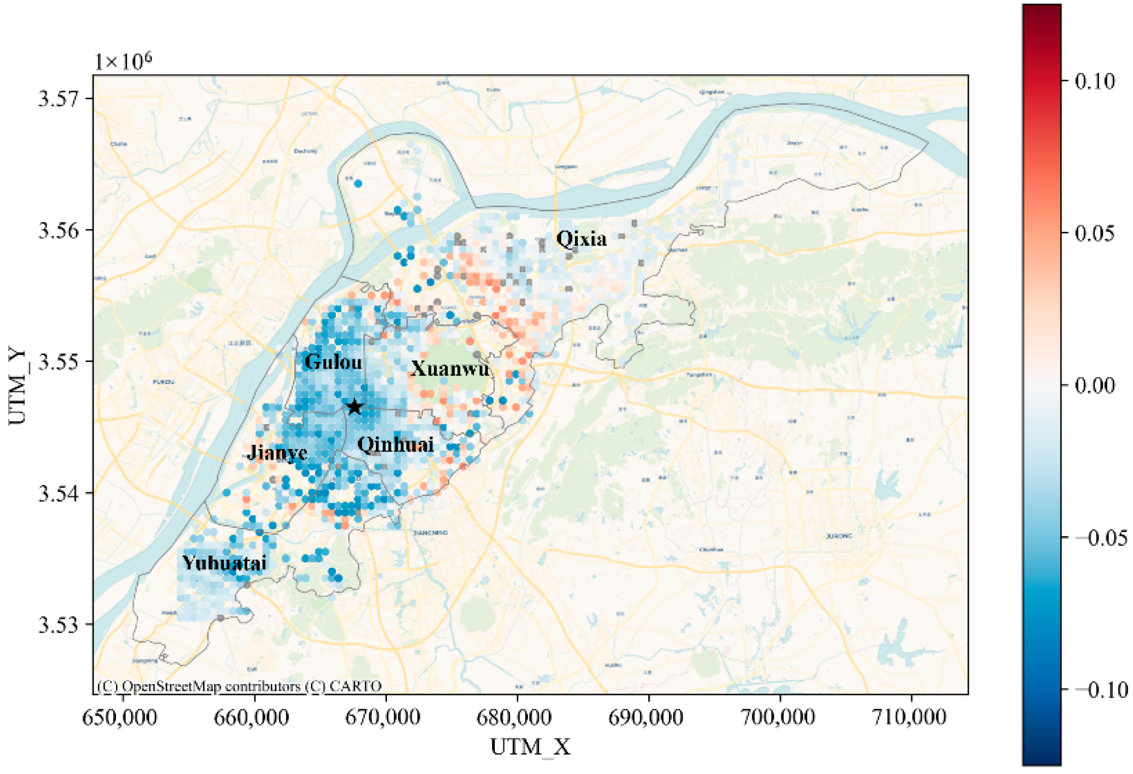
Figure 6 shows the interaction effects of DCC and geographic locations on ride-hailing. In Jianye, Gulou, and Qinhuai districts, the effects of DCC are significantly negative in general, indicating that ride-hailing demand increases as DCC increases. In the southern part of the Yuhuatai district and the northern part of the Qixia district, DCC exhibits a negative correlation with ride-hailing demand. This is likely caused by the lack of appeal for travel in these areas, somewhat reducing travel demand. In the southern part of the Qixia district, DCC positively impacts ride-hailing demand, meaning that as DCC increases, ride-hailing demand also increases. This is because the area has many educational and cultural institutions but has poor public transit systems, which in turn stimulates an increase in ride-hailing demand.
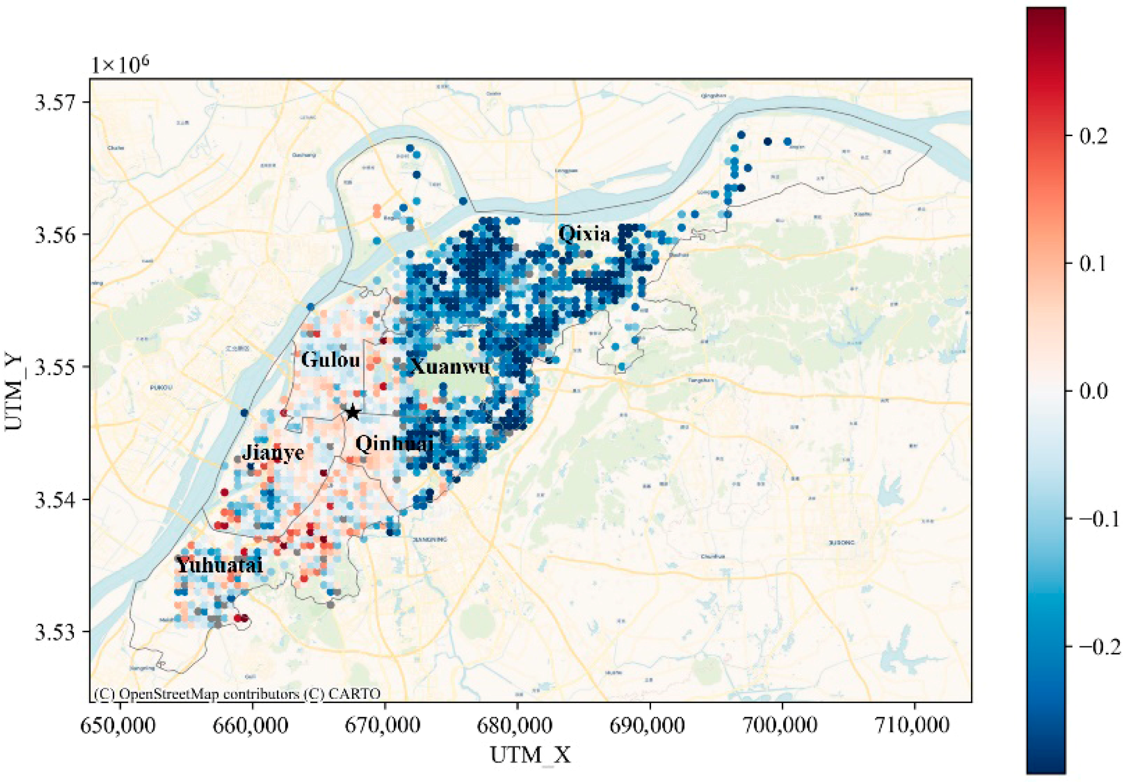
Figure 7 shows the effects of geographic locations on ride-hailing. In the boundary areas between the Jianye and Yuhuatai districts, as well as areas around the city center, the effects of geographic locations are positive. These areas feature by relatively dense population and higher LUM. The well-developed transport infrastructure in these areas offers favorable conditions for ride-hailing services, thereby enhancing the geographic values of these regions. Conversely, most areas in the Qixia district, as well as the peripheral areas of the Xuanwu and Qinhuai districts, significantly decrease ride-hailing demand.
Figure 8 shows the interaction effects of LUM and geographic locations on ride-hailing demand. The effects of LUM are generally negative in the peripheral areas (e.g., Yuhuatai and Qixia districts). In contrast, LUM positively influences ride-hailing demand in areas closer to the city center, such as Gulou, Jianye, and Qinhuai districts, indicating that higher land use diversity increases the usage of ride-hailing services. Additionally, it is observed that in some areas with relatively low LUM in the Yuhuatai district, there exists a positive relationship between the two issues. This finding can be attributed to the following reason: these areas are primarily a high-tech industrial zone with relatively single-function areas and insufficient transport infrastructure, and, thus, provide limited travel options.
Figure 9 shows the interaction effects of DMS and geographic locations. In most areas of the study region, a negative effect of DMS is observed. This finding may be explained by the competition and cooperative relationships between metro and ride-hailing services. In the core areas (e.g., Gulou district), due to the dense population, two transport modes have to cooperate to meet the travel needs. Thus, a large demand for ride-hailing services is generated although there exists higher subway accessibility. In contrast, in peripheral areas (e.g., Yuhuatai and Qixia districts), poorer metro accessibility forces people to use ride-hailing services to connect to the metro systems.

5. Conclusions

This study applies RF combined with GeoShapley to evaluate the effects of the BE on ride-hailing demand. It enriches the literature by examining the nonlinear and spatial interaction effects of the BE using ride-hailing order data from all transportation network companies in an entire city. The study offers several research and policy implications.
First, the study enriches the literature by quantifying the effects of the BE features on ride-hailing demand and examining their nonlinear patterns. The findings indicate that the LUM, interaction between DCC and geographic locations, and geographic locations rank the first three places in explaining ride-hailing demand. Additionally, all BE features exhibit nonlinear effects on ride-hailing demand and some of them show significant threshold effects. Specifically, RL and PD exhibit threshold effects at approximately 2 km and 15,000 persons, respectively, beyond which their effects on ride-hailing demand stabilize. LUM shows an inverted U-shaped relationship with ride-hailing demand, and the inflection point is at approximately 0.8. These findings offer implications for refined planning strategies.
Second, the study adds to prior research by capturing the interaction effects of the BE and geographic locations on ride-hailing demand. The GeoShapley method allows for incorporating geographic locations as a joint feature and demonstrates the spatial heterogeneity in ride-hailing demand. Additionally, the results of the interaction effects suggest that the effects of the BE features spatially vary across the city. Specifically, the effects of LUM are generally negative in the peripheral areas, whereas it positively influences ride-hailing demand in areas closer to the city center. This aligns with the results of prior studies [24]. The DCC only has positive effects in limited areas with many educational and cultural institutions and poor public transit systems. In most other areas, its effects are negative. These findings offer implications for implementing location-specific strategies.
Third, in terms of policy implications, the findings suggest that one-size-fits-all planning strategies may be ineffective. On the one hand, the findings indicate the necessity of optimizing the BE according to their importance and nonlinear effects. Planners and practitioners should prioritize improving key determinants within their most effective ranges. On the other hand, the effects of the BE features differ among geographic locations. The spatial varying effects indicate the importance of designing location-specific strategies tailored to local characteristics. In this regard, it is of importance for planners and practitioners to understand their complex relationships and design more refined planning strategies.
Some limitations should be acknowledged. First, the connection between the BE and ride-hailing may be sensitive to contexts. Thus, the findings based on data from a single city are difficult to generalize to other cities. More cross-city investigations should be considered in future work. Second, the study explores the short-term relationship between two issues, which restricts the ability to inform long-term BE planning strategies. In addition, the current study relies on a single-day dataset, which may not fully capture temporal variations in ride-hailing demand. This limitation calls for more investigations based on long-term data. Meanwhile, future research will further incorporate dynamic variables, such as real-time traffic congestion and weather conditions, to better identify the key factors influencing ride-hailing demand.

Author Contributions

Conceptualization, Y.G., Z.X., C.Y. and X.W.; Methodology, C.Y.; Validation, Y.G. and C.Y.; Formal analysis, Y.G., Z.X., C.Y. and X.W.; Investigation, Y.G. and Z.X.; Data curation, Y.G.; Writing—original draft, C.Y.; Writing—review and editing, X.W.; Supervision, Y.G. and X.W. All authors have read and agreed to the published version of the manuscript.

Funding

This work was sponsored by the National Natural Science Foundation of China (72204114, 52072025, 52202388) and the Humanities, Social Sciences Fund of the Ministry of Education of China (22YJC630191).

Data Availability Statement

The authors have no right to share the data because they belong to the research group, not only the authors.

Conflicts of Interest

The authors declare that they have no conflicts of interest.

Appendix A. Summary Statistics of GeoShapley Values

Min25%50%75%MaxMeanStdabs. Mean
LUM−0.863−0.222 0.122 0.177 0.254 −0.024 0.278 0.221
DCC × GEO−0.464 0.029 0.117 0.208 0.467 0.116 0.123 0.138
GEO−0.516 −0.204 −0.079 0.004 0.410 −0.095 0.135 0.129
DCC−0.312 −0.160 −0.066 0.045 0.294 −0.058 0.124 0.115
RL−0.473 −0.078 0.059 0.076 0.125 −0.003 0.127 0.100
DMS−0.275 −0.081 −0.006 0.074 0.227 −0.003 0.097 0.084
LUM × GEO−0.400 0.002 0.048 0.088 0.496 0.048 0.088 0.076
PD−0.100 −0.047 −0.032 0.050 0.160 −0.004 0.060 0.053
DBS−0.260 −0.009 0.011 0.038 0.075 −0.001 0.057 0.039
DMS × GEO−0.176 −0.019 0.004 0.034 0.153 0.006 0.047 0.035
RL × GEO−0.318 −0.014 0.004 0.029 0.320 0.006 0.046 0.032
PD × GEO−0.251 −0.017 0.002 0.026 0.262 0.008 0.046 0.030
HP−0.186 −0.005 0.005 0.012 0.065 −0.003 0.030 0.018
HP × GEO−0.172 −0.004 0.008 0.019 0.076 0.006 0.022 0.017
DBS × GEO−0.164 −0.009 0.002 0.013 0.152 0.001 0.025 0.017
BSD−0.012 −0.006 −0.001 0.006 0.058 0 0.007 0.006
BSD × GEO−0.040 −0.003 0 0.002 0.057 0 0.005 0.003
MSD−0.002 −0.001 −0.001 00.025 0 0.003 0.001
MSD × GEO−0.009 0000.019 0 0.001 0.001

References

  1. Lesteven, G.; Samadzad, M. Ride-hailing, a new mode to commute? Evidence from Tehran, Iran. Travel Behav. Soc. 2021, 22, 175–185. [Google Scholar] [CrossRef]
  2. Chung, J.; Namkung, O.S.; Ko, J.; Yao, E. Cycling distance and detour extent: Comparative analysis of private and public bikes using city-level bicycle trajectory data. Cities 2024, 151, 105134. [Google Scholar] [CrossRef]
  3. Wang, X.; Yin, C.; Zhang, J.; Shao, C.; Wang, S. Nonlinear effects of residential and workplace built environment on car dependence. J. Transp. Geogr. 2021, 96, 103207. [Google Scholar] [CrossRef]
  4. Zhao, F.; Ma, J.; Yin, C.; Tang, W.; Wang, X.; Yin, J. Spatiotemporal heterogeneous effects of built environment and taxi demand on ride-hailing ridership. Appl. Sci. 2024, 14, 142. [Google Scholar] [CrossRef]
  5. Ghaffar, A.; Mitra, S.; Hyland, M. Modeling determinants of ridesourcing usage: A census tract-level analysis of Chicago. Transp. Res. Part C Emerg. Technol. 2020, 119, 102769. [Google Scholar] [CrossRef]
  6. Zhao, D.; Yuan, Z.; Chen, M.; Yang, S. Differential pricing strategies of ride-sharing platforms: Choosing customers or drivers? Int. Trans. Oper. Res. 2022, 29, 1089–1131. [Google Scholar] [CrossRef]
  7. Yin, J.; Zhao, F.; Tang, W.; Ma, J. The Nonlinear and Threshold Effect of Built Environment on Ride-Hailing Travel Demand. Appl. Sci. 2024, 14, 4072. [Google Scholar] [CrossRef]
  8. Si, R.; Lin, Y.; Yang, D.; Guo, Q. Interpretable machine learning insights into the factors influencing residents’ travel distance distribution. ISPRS Int. J. Geo-Information 2025, 14, 39. [Google Scholar] [CrossRef]
  9. Yin, C.; Gui, C.; Xu, Z.; Shao, C.; Wang, X. Revisiting built environment and vehicle kilometer traveled: Does car ownership matter? Transp. Res. Part D Transp. Environ. 2025, 144, 104798. [Google Scholar] [CrossRef]
  10. Yin, C.; Shao, C. Revisiting commuting, built environment and happiness: New evidence on a nonlinear relationship. Transp. Res. Part D Transp. Environ. 2021, 100, 103043. [Google Scholar] [CrossRef]
  11. Ewing, R.; Cervero, R. Travel and the built environment: A meta-analysis. J. Am. Plan. Assoc. 2010, 76, 265–294. [Google Scholar] [CrossRef]
  12. Yin, C.; Zhang, J.; Shao, C.; Wang, X. Commute and built environment: What matters for subjective well-being in a household context? Transp. Policy 2024, 154, 198–206. [Google Scholar] [CrossRef]
  13. Wang, X.; Han, J.; Yin, C.; Shao, C.; Zhang, J. Built environment and travel satisfaction revisited: Differences between consonant and dissonant travelers. Transp. Res. Part A Policy Pract. 2025, 192, 104375. [Google Scholar] [CrossRef]
  14. Ding, C.; Wang, Y.; Tang, T.; Mishra, S.; Liu, C. Joint analysis of the spatial impacts of built environment on car ownership and travel mode choice. Transp. Res. Part D Transp. Environ. 2018, 60, 28–40. [Google Scholar] [CrossRef]
  15. Du, Q.; Zhou, Y.; Huang, Y.; Wang, Y.; Bai, L. Spatiotemporal exploration of the non-linear impacts of accessibility on metro ridership. J. Transp. Geogr. 2022, 102, 103380. [Google Scholar] [CrossRef]
  16. Newman, P. The environmental impact of cities. Environ. Urban. 2006, 18, 275–295. [Google Scholar] [CrossRef]
  17. Yin, C.; Wang, X.; Shao, C.; Ma, J. Exploring the relationship between built environment and commuting mode choice: Longitudinal evidence from China. Int. J. Environ. Res. Public Health 2022, 19, 14149. [Google Scholar] [CrossRef]
  18. Du, M.; Li, Z.; Li, X.; Xu, J.; Liu, D.; Kwan, M.P. Understanding the Spatial Variation of Integrated Use of Ride-Hailing Services With the Metro. J. Adv. Transp. 2024, 2024, 9210901. [Google Scholar] [CrossRef]
  19. Liu, Z.; Chen, H.; Sun, X.; Chen, H. Data-driven real-time online taxi-hailing demand forecasting based on machine learning method. Appl. Sci. 2020, 10, 6681. [Google Scholar] [CrossRef]
  20. Liu, Z.; Chen, H.; Li, Y.; Zhang, Q. Taxi demand prediction based on a combination forecasting model in hotspots. J. Adv. Transp. 2020, 2020, 1302586. [Google Scholar] [CrossRef]
  21. Liu, Z.; Chen, H. Short-term online taxi-hailing demand prediction based on the multimode traffic data in metro station areas. J. Transp. Eng. Part A Syst. 2022, 148, 05022003. [Google Scholar] [CrossRef]
  22. Wang, S.; Noland, R.B. Variation in ride-hailing trips in Chengdu, China. Transp. Res. Part D Transp. Environ. 2021, 90, 102596. [Google Scholar] [CrossRef]
  23. Sabouri, S.; Park, K.; Smith, A.; Tian, G.; Ewing, R. Exploring the influence of built environment on Uber demand. Transp. Res. Part D Transp. Environ. 2020, 81, 102296. [Google Scholar] [CrossRef]
  24. Yu, H.; Peng, Z.-R. Exploring the spatial variation of ridesourcing demand and its relationship to built environment and socioeconomic factors with the geographically weighted Poisson regression. J. Transp. Geogr. 2019, 75, 147–163. [Google Scholar] [CrossRef]
  25. Li, X.; Xu, J.; Du, M.; Liu, D.; Kwan, M.-P. Understanding the spatiotemporal variation of ride-hailing orders under different travel distances. Travel Behav. Soc. 2023, 32, 100581. [Google Scholar] [CrossRef]
  26. Alemi, F.; Circella, G.; Handy, S.; Mokhtarian, P. What influences travelers to use Uber? Exploring the factors affecting the adoption of on-demand ride services in California. Travel Behav. Soc. 2018, 13, 88–104. [Google Scholar] [CrossRef]
  27. Siddiq, F.; Taylor, B.D. A gendered perspective on ride-hail use in Los Angeles, USA. Transp. Res. Interdiscip. Perspect. 2024, 23, 100938. [Google Scholar] [CrossRef]
  28. Gomez, J.; Aguilera-García, Á.; Dias, F.F.; Bhat, C.R.; Vassallo, J.M. Adoption and frequency of use of ride-hailing services in a European city: The case of Madrid. Transp. Res. Part C Emerg. Technol. 2021, 131, 103359. [Google Scholar] [CrossRef]
  29. Yan, X.; Liu, X.; Zhao, X. Using machine learning for direct demand modeling of ridesourcing services in Chicago. J. Transp. Geogr. 2020, 83, 102661. [Google Scholar] [CrossRef]
  30. Zhang, B.; Chen, S.; Ma, Y.; Li, T.; Tang, K. Analysis on spatiotemporal urban mobility based on online car-hailing data. J. Transp. Geogr. 2020, 82, 102568. [Google Scholar] [CrossRef]
  31. Huang, G.; Qiao, S.; Yeh, A.G.-O. Spatiotemporally heterogeneous willingness to ridesplitting and its relationship with the built environment: A case study in Chengdu, China. Transp. Res. Part C Emerg. Technol. 2021, 133, 103425. [Google Scholar] [CrossRef]
  32. Dean, M.D.; Kockelman, K.M. Spatial variation in shared ride-hail trip demand and factors contributing to sharing: Lessons from Chicago. J. Transp. Geogr. 2021, 91, 102944. [Google Scholar] [CrossRef]
  33. Shen, X.; Zhou, Y.; Jin, S.; Wang, D. Spatiotemporal influence of land use and household properties on automobile travel demand. Transp. Res. Part D Transp. Environ. 2020, 84, 102359. [Google Scholar] [CrossRef]
  34. Liu, F.; Gao, F.; Yang, L.; Han, C.; Hao, W.; Tang, J. Exploring the spatially heterogeneous effect of the built environment on ride-hailing travel demand: A geographically weighted quantile regression model. Travel Behav. Soc. 2022, 29, 22–33. [Google Scholar] [CrossRef]
  35. Cao, Y.; Tian, Y.; Tian, J.; Liu, K.; Wang, Y.; Ustaoglu, E. Impact of built environment on residential online car-hailing trips: Based on MGWR model. PLoS ONE 2022, 17, e0277776. [Google Scholar] [CrossRef] [PubMed]
  36. Luo, Y.; Huang, A.; He, Z.; Zeng, J.; Wang, D. Exploring competitiveness of taxis to ride-hailing services from a multidimensional spatio-temporal perspective: A case study in Beijing, China. J. Transp. Geogr. 2024, 118, 103936. [Google Scholar] [CrossRef]
  37. Bi, H.; Ye, Z.; Zhu, H. Examining the nonlinear impacts of built environment on ridesourcing usage: Focus on the critical urban sub-regions. J. Clean. Prod. 2022, 350, 131314. [Google Scholar] [CrossRef]
  38. Li, W.; Zhao, S.; Ma, J.; Nielsen, O.A.; Jiang, Y. Book-ahead ride-hailing trip and its determinants: Findings from large-scale trip records in China. Transp. Res. Part A Policy Pract. 2023, 178, 103875. [Google Scholar] [CrossRef]
  39. Lai, J.; Wang, Y.; Yang, Y.; Wu, X.; Zhang, Y. Exploring the built environment impacts on Online Car-hailing waiting time: An empirical study in Beijing. Comput. Environ. Urban Syst. 2025, 115, 102205. [Google Scholar] [CrossRef]
  40. Li, W.; Ma, J.; Cai, H.; Chen, F.; Qin, W. The role of built environment in shaping reserved ride-hailing services: Insights from interpretable machine learning approach. Res. Transp. Bus. Manag. 2024, 56, 101173. [Google Scholar] [CrossRef]
  41. Ji, S.; Wang, X.; Lyu, T.; Liu, X.; Wang, Y.; Heinen, E.; Sun, Z. Understanding cycling distance according to the prediction of the XGBoost and the interpretation of SHAP: A non-linear and interaction effect analysis. J. Transp. Geogr. 2022, 103, 103414. [Google Scholar] [CrossRef]
  42. Peng, B.; Zhang, Y.; Li, C.; Wang, T.; Yuan, S. Nonlinear, threshold and synergistic effects of first/last-mile facilities on metro ridership. Transp. Res. Part D Transp. Environ. 2023, 121, 103856. [Google Scholar] [CrossRef]
  43. Wu, J.; Jia, P.; Feng, T.; Li, H.; Kuang, H. Spatiotemporal analysis of built environment restrained traffic carbon emissions and policy implications. Transp. Res. Part D Transp. Environ. 2023, 121, 103839. [Google Scholar] [CrossRef]
  44. Yin, C.; Zhang, J.; Shao, C. Relationships of the multi-scale built environment with active commuting, body mass index, and life satisfaction in China: A GSEM-based analysis. Travel Behav. Soc. 2020, 21, 69–78. [Google Scholar] [CrossRef]
  45. Wang, X.; Wang, W.; Yin, C.; Shao, C.; Luo, S.; Liu, E. Relationships of life satisfaction with commuting and built environment: A longitudinal analysis. Transp. Res. Part D Transp. Environ. 2023, 114, 103513. [Google Scholar] [CrossRef]
  46. Wang, X.; Shao, C.; Yin, C.; Guan, L. Built environment, life events and commuting mode shift: Focus on gender differences. Transp. Res. Part D Transp. Environ. 2020, 88, 102598. [Google Scholar] [CrossRef]
  47. Ewing, R.; Cervero, R. Travel and the built environment: A synthesis. Transp. Res. Rec. J. Transp. Res. Board 2001, 1780, 87–114. [Google Scholar] [CrossRef]
  48. Agarwal, S.; Charoenwong, B.; Cheng, S.-F.; Keppo, J. The impact of ride-hail surge factors on taxi bookings. Transp. Res. Part C: Emerg. Technol. 2022, 136, 103508. [Google Scholar] [CrossRef]
  49. Yang, L.; Yu, B.; Liang, Y.; Lu, Y.; Li, W. Time-varying and non-linear associations between metro ridership and the built environment. Tunn. Undergr. Space Technol. 2023, 132, 104931. [Google Scholar] [CrossRef]
  50. Li, Z. GeoShapley: A Game Theory Approach to Measuring Spatial Effects in Machine Learning Models. Ann. Assoc. Am. Geogr. 2024, 114, 1365–1385. [Google Scholar] [CrossRef]
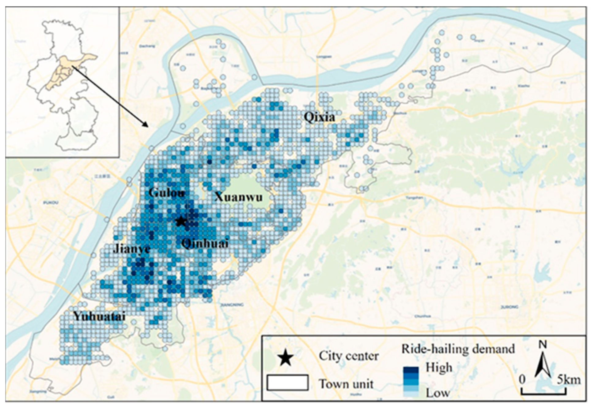
Figure 1. Ride-hailing demand in the study region.
Buildings 15 02967 g001
Figure 2. Research framework.
Buildings 15 02967 g002
Figure 3. Correlation matrix of features.
Buildings 15 02967 g003
Figure 4. Feature importance ranking and GeoShapley values.
Buildings 15 02967 g004
Figure 5. Nonlinear effects of the BE on ride-hailing demand.
Buildings 15 02967 g005
Figure 6. Interaction effects of DCC and geographic locations.
Buildings 15 02967 g006
Figure 7. Effects of geographic locations.
Buildings 15 02967 g007
Figure 8. Interaction effects of LUM and geographic locations.
Buildings 15 02967 g008
Figure 9. Interaction effects of DMS and geographic locations.
Buildings 15 02967 g009
Table 1. Descriptive characteristics of variables.
VariablesDescriptionMeanSt. Dev.
Dependent variables
Ride-hailing demandRide-hailing travel demand of all transportation network companies within each grid (count)69.4599.74
Independent variable
Density
Population density (PD)The population size within the grid (persons)29804737
Design
Road length (RL)The road length within the grid (km)2.491.39
Diversity
Land use mixture (LUM)The entropy index of the 7 types of POIs within the grid0.770.25
Destination accessibility
Distance to city center (DCC)Euclidean distance from the city center (km)10.556.03
Distance to transit
Distance to bus stop (DBS)Euclidean distance from the nearest bus stop (km)0.330.25
Distance to metro stop (DMS)Euclidean distance from the nearest metro stop (km)1.571.62
Bus stop density (BSD)The number of bus stops within the grid (count)0.931.11
Metro stop density (MSD)The number of metro stops within the grid (count)0.060.24
Demographic
Housing price (HP)The average residential HP within the grid (ten thousand yuan)3.321.17
Geographic location
UTM_XThe longitude of the grid centroid point671,093.748648.63
UTM_YThe latitude of the grid centroid point3,547,446.487896.26
Table 2. Model results.
R2RMSEMAE
RF0.6250.4980.395
XGBoost0.5760.5300.415
GWR0.5770.5030.401
Disclaimer/Publisher’s Note: The statements, opinions and data contained in all publications are solely those of the individual author(s) and contributor(s) and not of MDPI and/or the editor(s). MDPI and/or the editor(s) disclaim responsibility for any injury to people or property resulting from any ideas, methods, instructions or products referred to in the content.