Article

Machine Learning-Based Surrogate Ensemble for Frame Displacement Prediction Using Jackknife Averaging

1
School of Statistics, Capital University of Economics and Business, Beijing 100070, China
2
Tongzhou Campus Construction Department, Renmin University of China, Beijing 100872, China
3
School of Economics, Capital University of Economics and Business, Beijing 100070, China
*
Author to whom correspondence should be addressed.
Buildings 2025, 15(16), 2872; https://doi.org/10.3390/buildings15162872 (registering DOI)
Submission received: 30 June 2025 / Revised: 10 August 2025 / Accepted: 12 August 2025 / Published: 14 August 2025

Abstract

High-fidelity finite element analysis (FEA) plays a key role in structural engineering by enabling accurate simulation of displacement, stress, and internal forces under static loads. However, its high computational cost limits applicability in real-time control, iterative design, and large-scale uncertainty quantification. Surrogate modeling provides a computationally efficient alternative by learning input–output mappings from precomputed simulations. Yet, the performance of individual surrogates is often sensitive to data distribution and model assumptions. To enhance both accuracy and robustness, we propose a model averaging framework based on Jackknife Model Averaging (JMA) that integrates six surrogate models: polynomial response surfaces (PRSs), support vector regression (SVR), radial basis function (RBF) interpolation, eXtreme Gradient Boosting (XGB), Light Gradient Boosting Machine (LGBM), and Random Forest (RF). Three ensembles are formed: JMA1 (classical models), JMA2 (tree-based models), and JMA3 (all models). JMA assigns optimal convex weights using cross-validated out-of-fold errors without a meta-learner. We evaluate the framework on the Static Analysis Dataset with over 300,000 FEA simulations. Results show that JMA consistently outperforms individual models in root mean squared error, mean absolute error, and the coefficient of determination, while also producing tighter, better-calibrated conformal prediction intervals. These findings support JMA as an effective tool for surrogate-based structural analysis.

1. Introduction

Structural static analysis is a foundational technique of civil and mechanical engineering, playing a vital role in assessing the safety, stability, and performance of load-bearing structures. Static finite element analysis (FEA) has become the principal methodology for computing structural responses under static load or equivalent static load effects—such as internal forces, displacements, and stresses [1,2]. This simulation technique allows detailed modeling of complex geometries and heterogeneous material behavior, making it indispensable for modern structural analysis and design.
However, high-fidelity FEA models can involve thousands to millions of degrees of freedom (DOF), especially when fine meshing or complex physics is considered. As a result, repeated simulations required for design optimization, uncertainty quantification, or real-time monitoring often become computationally intractable [3,4].
To address this challenge, surrogate modeling has emerged as a practical and scalable solution. Surrogate models aim to approximate the input–output behavior of FEA solvers using data-driven learning techniques based on a limited number of simulations. Classical surrogate approaches, including polynomial response surfaces (PRSs) [5,6], radial basis function (RBF) interpolation [7,8], and support vector regression (SVR) [9,10], are widely applied in engineering due to their simplicity and interpretability. At the same time, tree-based ensemble methods such as eXtreme Gradient Boosting (XGB) [11], Light Gradient Boosting Machine (LGBM) [12], and Random Forests (RFs) [13] have shown strong performance by offering nonlinear modeling capabilities, robustness to noise, and automated feature selection.
Nonetheless, in complex simulation settings with high-dimensional sparse inputs and localized nonlinearities, the predictive performance of a single model can vary significantly across tasks. Model instability, overfitting, and structural misspecification remain key challenges. This motivates the use of ensemble strategies that can combine the strengths of different models to improve generalization and reduce variance.
Model averaging is a promising strategy that provides a theoretically grounded framework for combining multiple candidate models through convex weighting. Jackknife Model Averaging (JMA), proposed by [14], determines model weights by minimizing the leave-one-out cross-validation error. It enjoys strong theoretical properties, including asymptotic optimality even in the presence of model misspecification and heteroskedasticity [15]. A key advantage of JMA lies in its flexibility; unlike traditional tree ensembles, it is not limited to models of the same type. Instead, it can integrate a wide variety of models, including linear models, kernel-based approaches, tree-based methods, and neural networks. This flexibility makes JMA especially well-suited for hybrid surrogate modeling.
JMA has been successfully applied in various domains, including economic forecasting [16], dependent time series [17], high-dimensional regression [18], quantile modeling [19], and medical prognosis [20]. Nevertheless, its use in structural engineering remains limited, particularly in the context of surrogate modeling for FEA.
In this work, we bridge this gap by applying JMA to predict the maximum displacement response in static structural analysis. We conduct extensive experiments using the Static Analysis Dataset (StAnD) [21], which contains over 300,000 finite element simulations of frame structures subjected to static loads such as gravity, lateral forces, and uniformly distributed loads. The dataset provides a diverse and realistic testbed for evaluating surrogate models in complex structural settings.
To assess the benefits of JMA under different ensemble configurations, we consider the following three model combinations:
  • JMA1: Classical surrogates—PRS, RBF, and SVR.
  • JMA2: Tree-based models—XGB, LGBM, and RF.
  • JMA3: Hybrid combination—all six models.
Our contributions are summarized as follows:
  • We benchmark the predictive performance of six representative surrogate models on a large-scale, realistic structural simulation dataset.
  • We design and compare three model averaging strategies (JMA1, JMA2, and JMA3) to evaluate the benefits of homogeneous versus hybrid ensembles.
  • We show that JMA-based ensembles consistently achieve superior accuracy, robustness, and generalization.
The remainder of this paper is organized as follows. Section 2 introduces the structural displacement prediction task and describes the simulation dataset used in this study. Section 3 reviews six widely used surrogate modeling techniques that form the basis for ensemble construction. In Section 4, we detail the proposed methodology, including the formal setup of the surrogate modeling problem, the selection of base learners, and the implementation of the JMA framework. Section 5 presents the experimental design, evaluation metrics, and analysis of predictive performance and uncertainty quantification. Section 6 concludes this paper with a summary of key findings and future research directions.

2. Problem Definition and Data Description

This study leverages the StAnD, a large-scale simulation dataset specifically designed to benchmark surrogate modeling and sparse linear solvers in structural analysis. Each instance in the dataset represents a static FEA problem involving a randomly generated steel frame subjected to realistic static loads.

2.1. Problem Definition

Each problem in the StAnD dataset corresponds to the numerical solution of a sparse linear system of the form
K u = F ,
where K R n × n is the global stiffness matrix, u R n is the nodal displacement vector (solution), and F R n is the external force vector. The matrix K is symmetric and positive definite and is stored in compressed coordinate format for efficient handling of sparsity.
Each simulation instance is stored as a separate .npz file and includes the following components:
  • A_indices: A ( 2 , nnz ) array of integer-valued row and column indices of non-zero entries in K;
  • A_values: A ( nnz ) array containing the corresponding non-zero values of K;
  • b: A length-n vector representing the right-hand-side load vector F;
  • x: A length-n vector representing the displacement solution u , obtained by solving the linear system.
The full dataset is partitioned into training and test subsets. In this work, we focus on the stand_small_train (100,000 samples) and stand_small_test (1000 samples) partitions for model training and evaluation, respectively.

2.2. Feature Construction

To enable regression-based surrogate modeling, each simulation instance is transformed into a structured input–output pair ( x i , y i ) . The input feature vector x i R 6 summarizes the numerical properties of the stiffness matrix K and the force vector F, while the scalar response y i is defined as the maximum absolute displacement:
y i = max j | u i j | .
The following features are extracted to characterize the structural system and loading condition:
  • b_mean, b_std, b_max, and b_nnz: The mean, standard deviation, maximum absolute value, and number of non-zero entries in the force vector F;
  • A_abs_sum and A_nnz: The total sum of absolute values and the number of non-zero entries in the stiffness matrix K.
These six features collectively capture both the magnitude and sparsity patterns of the loading and structural system, providing a compact yet informative representation suitable for data-driven surrogate modeling.

2.3. Use Case Motivation

Frame structures are the most commonly used structural systems in multistory buildings. For such structures, larger cross-sectional dimensions of structural members lead to greater structural stiffness. Achieving a reasonable level of structural stiffness is often a central objective in structural design. If the cross-section is too large, the structure becomes uneconomical; if it is too small, it may fail to ensure safety. Given the building’s height, geometry, number of floors, and load distribution, it is possible to use algorithms to predict a reasonable range of structural stiffness. This enables rapid estimation of suitable structural member sizes, significantly reducing the effort required for model calibration while playing a critical role in ensuring both safety and economic efficiency.
For a frame structure under lateral load (as shown in Figure 1, the lateral displacement of the center of mass under load F is given by model (1). In FEA of frame structures, each nodal point is characterized by six degrees of freedom (three translational and three rotational). This formulation results in a rapid dimensional expansion of the global stiffness matrix proportional to the number of nodes. Such dimensional growth not only substantially increases memory allocation requirements for finite element computations but also induces a superlinear scaling of solution time with respect to nodal count. This exponential increase in computational complexity presents a fundamental challenge in achieving refined analytical precision during frame structure design processes.
FEA can provide internal forces and deformations of the structure under different loading conditions. This is crucial for evaluating load-bearing capacity and structural safety. Static analysis helps determine whether a structure has sufficient stiffness to resist deformation and whether it has adequate strength to avoid failure under the design load.
In structural static analysis, the loads considered typically include permanent loads, such as the self-weight of the structure, live loads, including uniformly distributed loads, and wind loads. These loads can be applied in various forms, including concentrated forces, uniform distributions, bending moments, prescribed displacements, and thermal actions. Within the framework of linear static analysis, the material is assumed to behave elastically, and the structure is analyzed under the assumption that it remains within the elastic range. As a result, the structural response exhibits a linear relationship with the applied loads, allowing for the direct evaluation of stiffness and strength under a given loading scenario.

2.4. Dataset Description

The dataset employed in this study is the StAnD dataset, which comprises finite element static analysis results for a large collection of frame structures. The structural models were programmatically generated using OpenSeesPy (v3.5.0, Python 3.11.4), the Python interface for the OpenSees finite element solver. Based on the principle of superposition, static loads were separately applied to the simulated models to calculate structural displacements under different loading conditions. In total, the dataset includes 303,000 samples, which are grouped according to the number of DOF in each structure—equivalent to the dimension of the global stiffness matrix. Specifically, the dataset contains small-scale models with an average of 2115 DOF, medium-scale models with approximately 7000 DOF, and large-scale models averaging around 15,500 DOF. This study focuses on a subset of 100,000 samples drawn from the small-scale group.
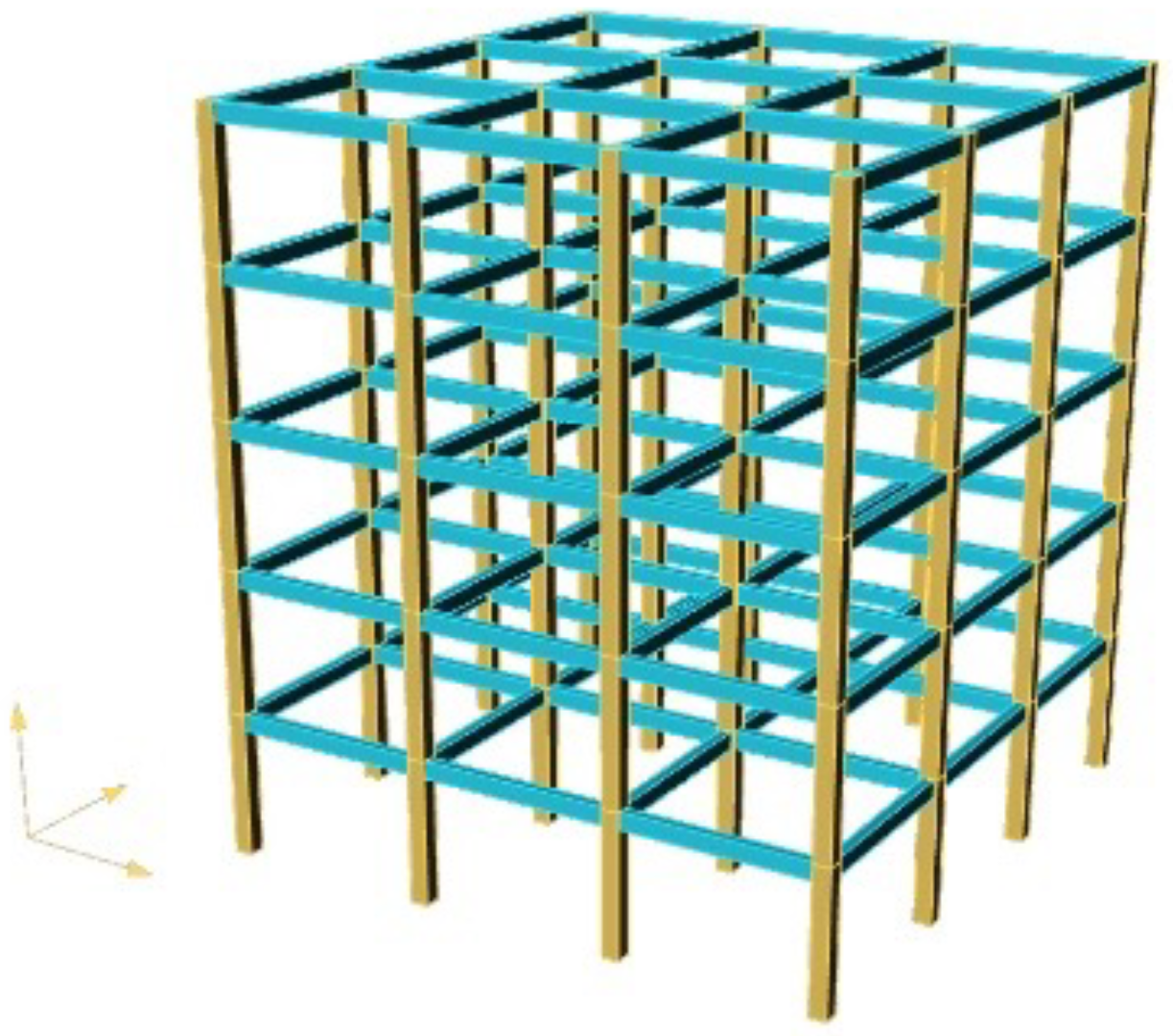
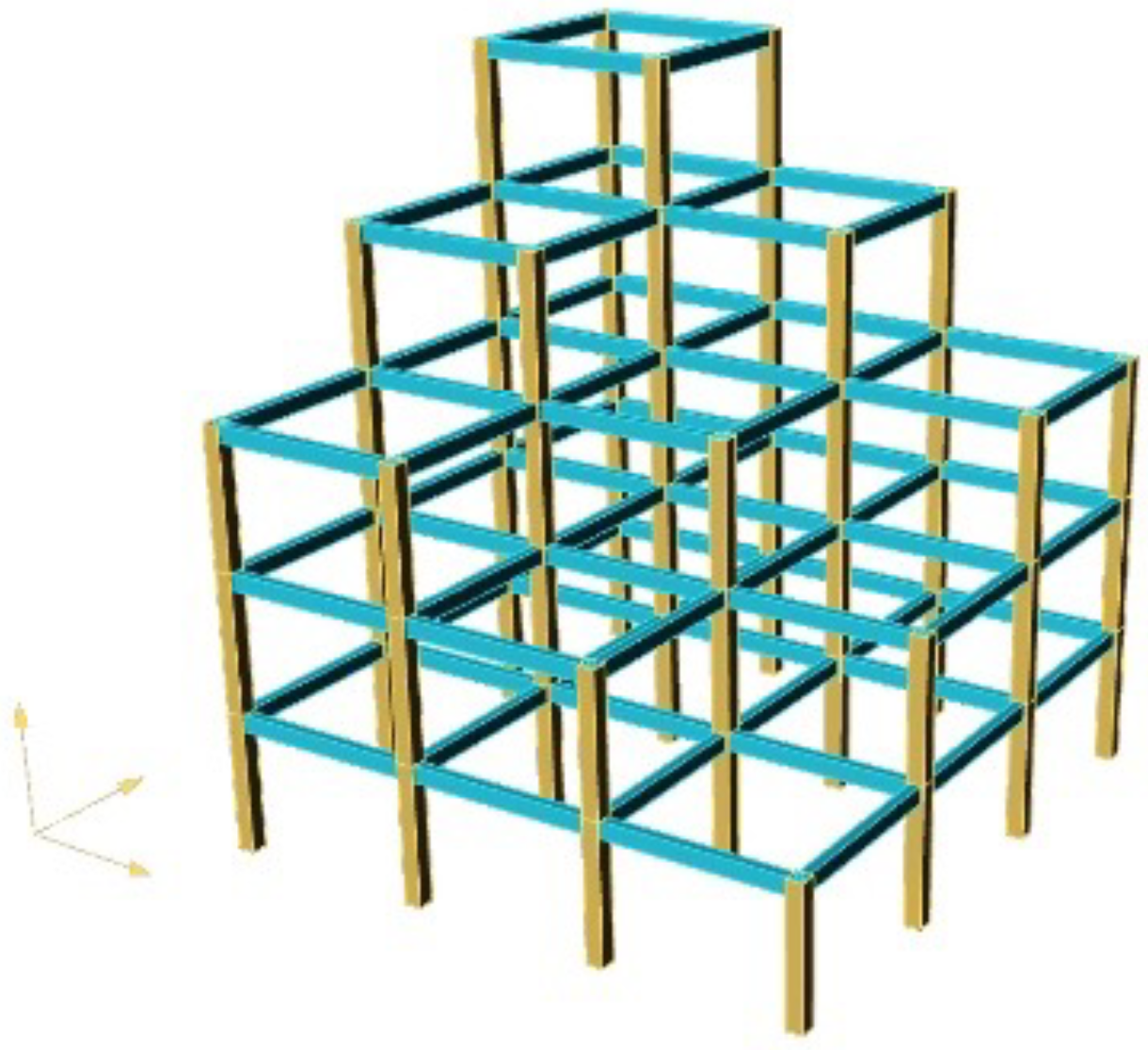
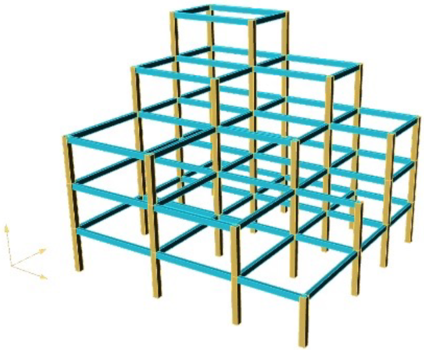
Each frame model is constructed from a regular three-dimensional grid composed of B × D × H unit cubes. The values of B, D, and H are uniformly sampled within predefined ranges to determine the initial model dimensions consistent with the target DOF. To introduce variability in structural geometry, a random number of cubes—ranging from 0 to H—are removed from the top layer of the grid, creating structures with varying heights. Subsequently, the remaining cubes are modified such that the thickness of their horizontal faces (orthogonal to a specified direction) is randomly assigned a value between 3 and 6 m, replacing the default unit thickness of 1 m. The geometric characteristics of representative frame structures with increasing levels of complexity are illustrated in Figure 2, Figure 3 and Figure 4.
Each simulation in the dataset corresponds to one instance of the linear system defined in Equation (1) and includes the full tuple ( K , F , u ) . The structural members are modeled as Timoshenko beams, with geometric and material parameters (length: 3–6 m; width: 0.2–0.4 m; height: 0.4–0.6 m; Young’s modulus: 2.5 × 10¹⁰ to 4.3 × 10¹⁰ Pa; and density: 2000 to 2600 kg/m3) randomly sampled from realistic ranges.
Further details regarding the simulation method and loading conditions are provided below to clarify how the dataset was constructed.
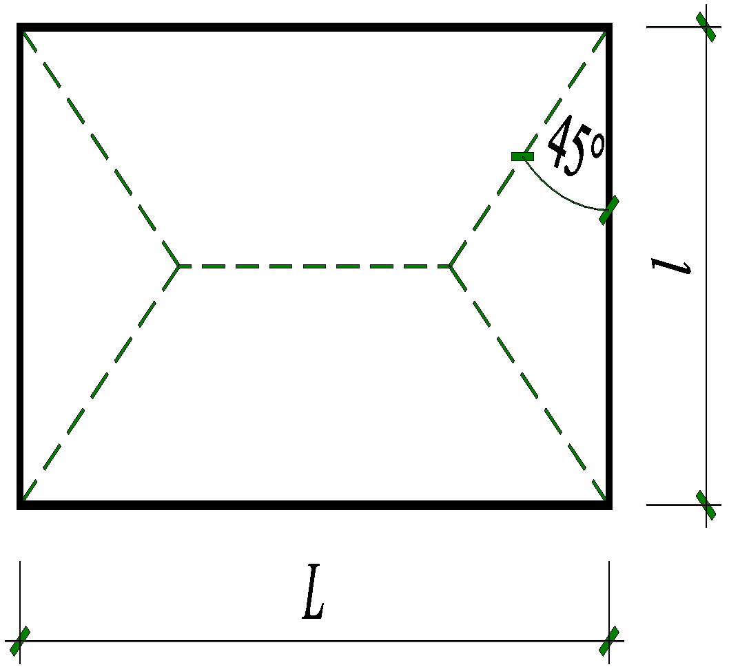
The static loads considered in the analysis include structural self-weight, additional permanent loads, floor live loads, and wind loads, with wind loads determined in accordance with the relevant Italian building codes. The self-weight of the frame is applied as line loads along the structural members, calculated by multiplying the cross-sectional area of each member by the material density. Floor slabs are modeled using four-node elements. The self-weight and uniformly distributed live loads on the slabs are transferred to the surrounding beams through triangular and trapezoidal load distribution schemes and then applied as uniformly distributed line loads on the beams. As illustrated in the diagram below, for a slab with a uniformly distributed load q, the equivalent line load on the short-span beam is q l / 4 , while the equivalent line load on the long-span beam is q l ( L l / 2 ) / ( 2 L ) , where l and L represent the short and long span lengths, respectively. The assumed load transfer mechanism from the slab to the surrounding beams and the corresponding equivalent line loads are illustrated in Figure 5 and Figure 6.

2.5. Exploratory Analysis of Data Distribution

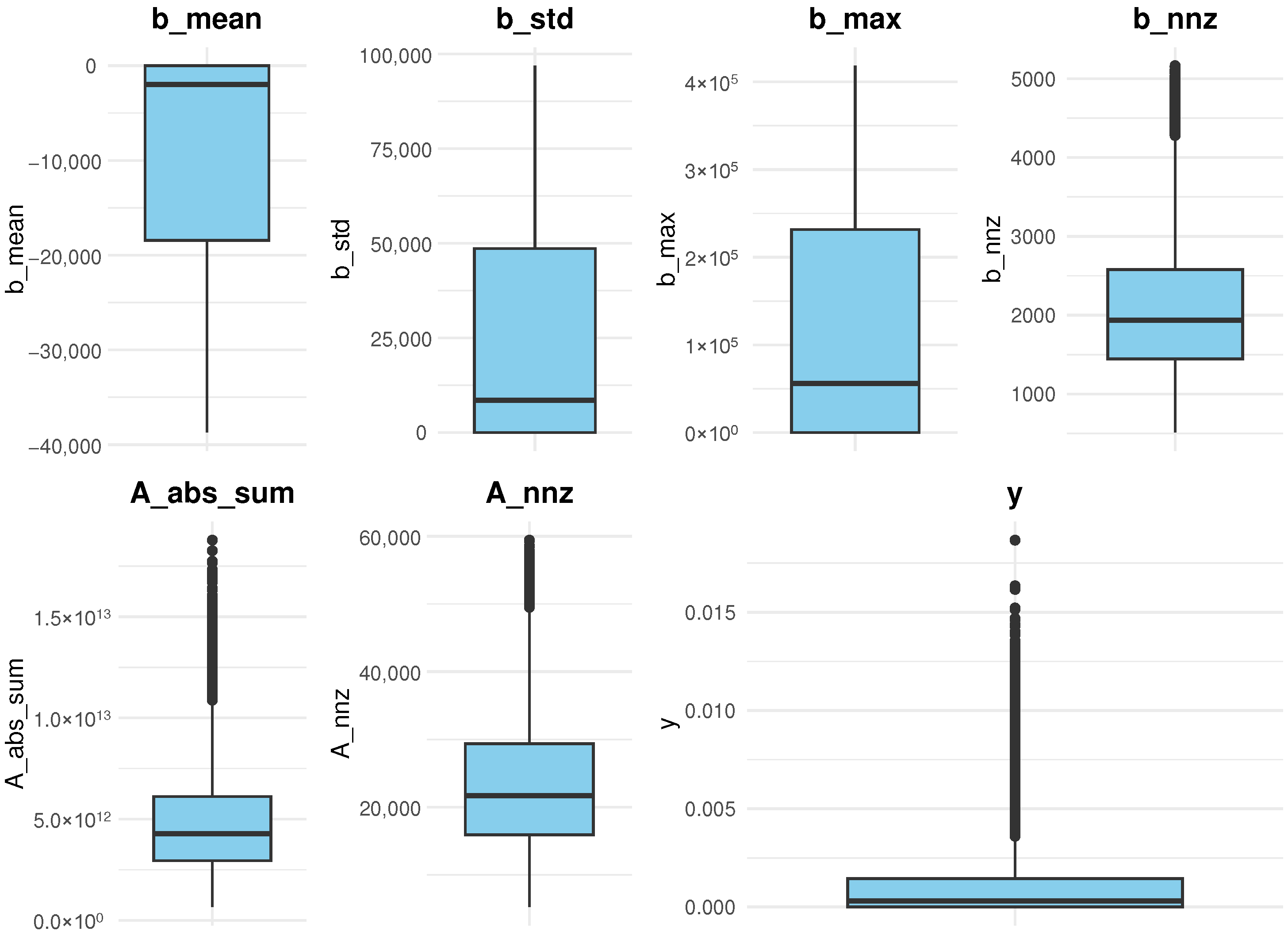
To gain insights into the characteristics of the training data, we present an exploratory analysis of the input features and the response variable. Figure 7 displays the boxplots of six key structural features: b_mean, b_std, b_max, b_nnz, A_abs_sum, and A_nnz. The figure also includes the scalar response y, which is defined as the maximum absolute displacement.
The distributions reveal varying scales and dispersion across features. For example, b_std and b_max exhibit large variability with noticeable skewness, while b_mean shows a concentration of values below zero. Both A_abs_sum and A_nnz display heavy-tailed distributions, indicating the presence of highly complex structures. The response variable y is also right-skewed, with most values concentrated near zero and a small number of large-displacement outliers.
This analysis highlights the heterogeneity and potential imbalance in the dataset. Such characteristics may affect model performance and training dynamics. Some individual models are more robust to these irregularities, which is reflected in their relative weightings in the proposed model aggregation framework.

3. Related Models

In this section, we provide a brief overview of the surrogate models and tree-based models considered in this study. Specifically, PRS, SVR, and RBF are categorized as surrogate models, while XGB, LGBM, and RF are tree-based ensemble models. The algorithmic flowcharts corresponding to these models are presented in Figure 8, Figure 9, Figure 10, Figure 11, Figure 12 and Figure 13.

3.1. PRS Model

PRS modeling is a widely used surrogate modeling technique for efficiently approximating complex input–output relationships in engineering design, reliability analysis, and uncertainty quantification. Originating from the classical Response Surface Methodology proposed by [22], PRS has been further developed and formalized in subsequent works [6]. The main objective of PRS is to construct an explicit polynomial approximation of a computationally expensive or implicitly defined system based on a finite set of simulation or experimental data.
In this study, a second-order (full quadratic) PRS model is employed, which takes the following general form:
y ^ ( x ) = β 0 + i = 1 d β i x i + i = 1 d β i i x i 2 + 1 i < j d β i j x i x j ,
where x = ( x 1 , x 2 , , x d ) denotes the vector of input variables, y ^ is the predicted response, and β represents the regression coefficients. These coefficients are estimated using ordinary least squares (OLS) by minimizing the sum of squared residuals between the observed and predicted values.
The construction and application of the PRS model in this work follow these steps:
  • Problem definition: Identify the modeling objective, input variables, and constraints.
  • Data selection: Use all available training data without experimental design subsampling.
  • Model fitting: Fit a full quadratic polynomial regression using the ordinary least squares method.
  • Model validation: Assess goodness of fit using criteria such as adjusted R 2 ( R a d j 2 ), predictive Q 2 , and analysis of variance (ANOVA).
  • Analysis or optimization: Apply the surrogate model for optimization, sensitivity analysis, or uncertainty quantification as required.
By mapping complex nonlinear system behavior into a polynomial form, PRS models enable rapid evaluation, optimization, and sensitivity analysis, while maintaining interpretability and low computational cost. Nevertheless, the accuracy of PRS models may degrade in highly nonlinear, discontinuous, or high-dimensional problems due to the curse of dimensionality.

3.2. RBF Surrogates

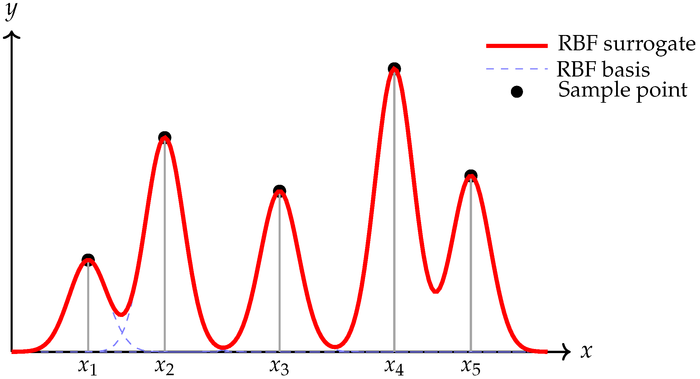
RBF surrogates are interpolation models widely employed for approximating computationally intensive or complex response surfaces in engineering design, numerical optimization, and uncertainty quantification [7]. The fundamental principle behind RBF surrogates is representing the target function as a linear combination of radially symmetric basis functions, each centered at sampled data points.
Formally, an RBF surrogate is defined as follows:
y ^ ( x ) = i = 1 n w i ϕ x x i ,
where x i denotes sampled input points, w i represents weighting coefficients, and ϕ ( · ) is the chosen RBF. Common RBFs include Gaussian ( ϕ ( r ) = exp ( γ r 2 ) ), Multiquadric ( ϕ ( r ) = r 2 + γ 2 ), and thin-plate splines ( ϕ ( r ) = r 2 ln ( r ) ).
Weights w i are determined by enforcing exact interpolation conditions:
y ^ ( x i ) = y i , i = 1 , , n ,
leading to the linear system
Φ w = y ,
with interpolation matrix entries Φ i j = ϕ ( x i x j ) .
RBF surrogates are particularly effective for interpolating deterministic simulations or functions exhibiting smooth behavior. However, standard RBF interpolation may lead to overfitting when applied to noisy data, in which case regularized or smoothing RBF approaches are recommended.
Each RBF is localized around a sampled data point, influencing the surrogate locally. The RBF surrogate (red curve) precisely interpolates all observed data points. In practical applications with noisy data, a smoothing (regularized) RBF approach is often adopted to enhance the model’s predictive capability and avoid overfitting.

3.3. SVR

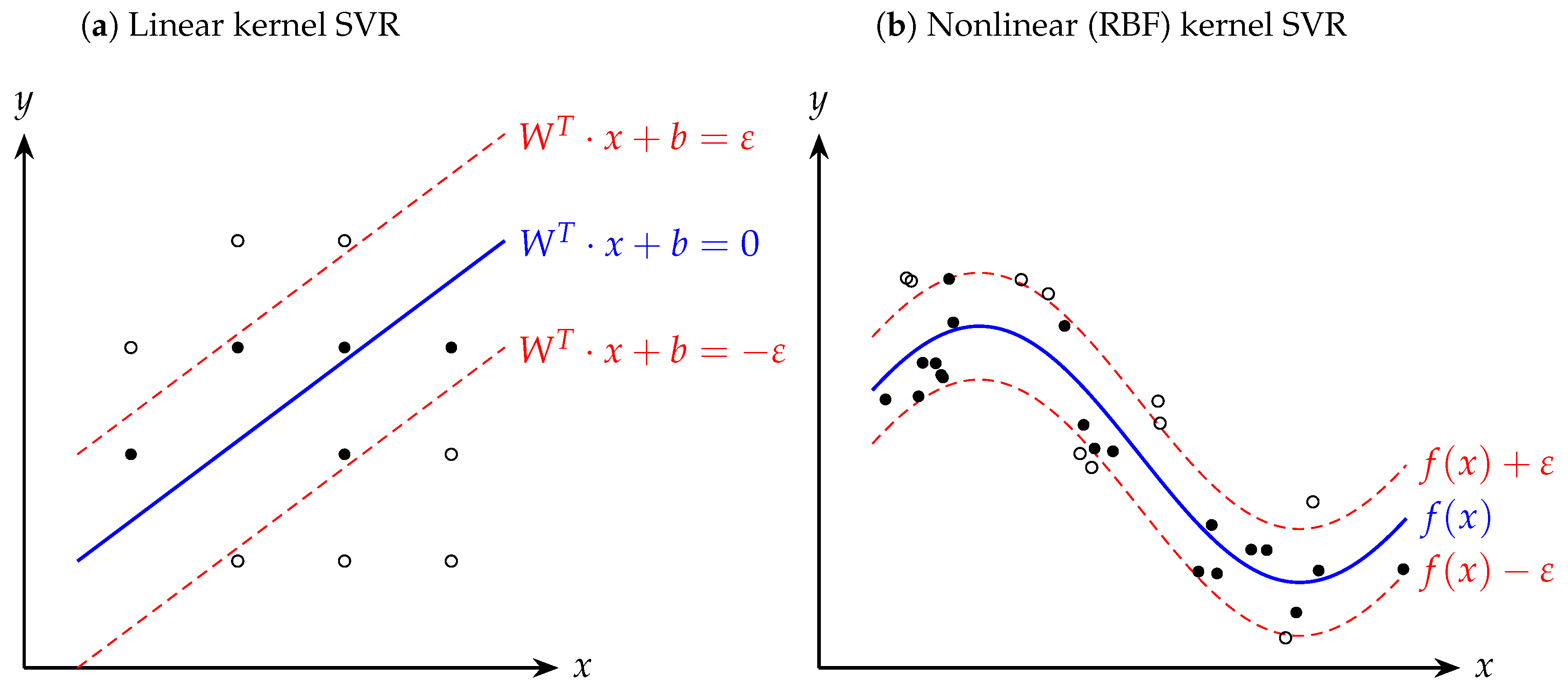
SVR is a kernel-based supervised learning algorithm developed as the regression extension of Support Vector Machines, originally introduced by Vapnik and colleagues and popularized by [9]. Unlike traditional least squares regression, which minimizes the total squared error, SVR aims to find a predictive function f ( x ) = w , ϕ ( x ) + b that approximates the underlying relationship within an ε -insensitive margin while promoting model flatness and sparsity.
The SVR training problem is formulated as the following convex optimization:
min w , b , ξ i , ξ i 1 2 w 2 + C i = 1 n ( ξ i + ξ i ) s . t . y i w , ϕ ( x i ) b ε + ξ i , w , ϕ ( x i ) + b y i ε + ξ i , ξ i , ξ i 0 , i = 1 , , n ,
where ϕ ( · ) denotes a mapping from input space to a high-dimensional feature space, C is the regularization parameter, and ε specifies the margin of tolerance for prediction errors.
In practice, SVR leverages the kernel trick to avoid explicit computation in the high-dimensional feature space. A commonly used kernel is the RBF kernel:
K ( x i , x j ) = exp ( γ x i x j 2 ) ,
where γ > 0 is a kernel width parameter. The choice of kernel determines whether the model captures linear or nonlinear relationships in the data.
Owing to its robust generalization performance and capability to capture nonlinear dependencies with limited training data, SVR has been extensively applied in engineering fields such as structural reliability analysis, uncertainty quantification, and damage detection [23,24,25]. Its seamless integration into surrogate modeling frameworks makes SVR a compelling choice for approximating complex finite element simulations and other computationally intensive engineering systems.

3.4. XGB

XGB, proposed by [11], is an efficient and scalable implementation of gradient-boosted decision trees. It leverages the gradient boosting framework, constructing an ensemble of weak learners—typically regression trees—in a sequential, stage-wise manner to minimize a differentiable loss function. At each iteration, XGB adds a new tree trained on the negative gradient (residual) of the loss function relative to the existing ensemble predictions, incrementally enhancing model performance.
Formally, let y ^ i ( t ) denote the prediction at the t-th boosting iteration. XGB minimizes the following objective function:
L ( t ) = i = 1 n y i , y ^ i ( t 1 ) + f t ( x i ) + Ω ( f t ) ,
where is a convex loss function, f t F represents the regression tree fitted at iteration t, and the regularization term Ω ( f ) is defined as
Ω ( f ) = γ T + 1 2 λ j = 1 T w j 2 .
Here, T denotes the number of leaves in the tree and w j represents the weights of the leaves. This regularization mechanism penalizes tree complexity to mitigate overfitting and improve generalization.
XGB incorporates several algorithmic innovations that significantly enhance its computational efficiency and predictive accuracy, including a regularized learning objective to control model complexity, a sparsity-aware tree-splitting algorithm robust to missing values, parallelized tree construction with cache-aware data structures for accelerated computation, and column subsampling and early stopping methods to enhance model robustness and reduce computational overhead.
Due to its superior accuracy, interpretability, and scalability, XGB has seen widespread adoption across various scientific and engineering disciplines. Particularly in structural mechanics, XGB is employed for rapid prediction of simulation outcomes, efficient damage localization, and effective uncertainty quantification under conditions characterized by high dimensionality and nonlinearity.

3.5. LGBM

LGBM, proposed by [12], is an advanced gradient boosting framework specifically designed for efficient handling of large-scale, high-dimensional datasets. It has rapidly gained popularity across various domains, from industrial applications and financial modeling to competitive data science platforms such as Kaggle, due to its superior speed, memory efficiency, and predictive accuracy [26,27,28]. LGBM’s computational efficiency makes it particularly suitable for real-time prediction scenarios and resource-constrained environments, such as Internet of Things (IoT) systems, real-time anomaly detection, and financial risk modeling [29,30].
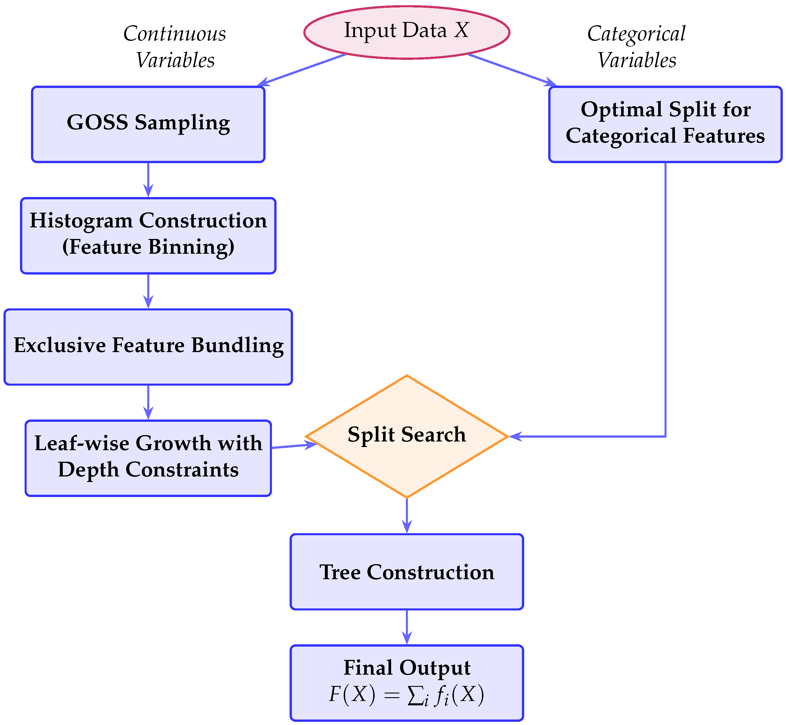
The framework introduces three key algorithmic innovations: (i) a histogram-based decision tree algorithm, (ii) Gradient-based One-Side Sampling (GOSS), and (iii) Exclusive Feature Bundling (EFB). The histogram-based approach discretizes continuous features into fixed bins, enabling efficient computation of feature splits using precomputed statistics, significantly reducing memory usage [12]. GOSS strategically retains samples with large gradients—those contributing significantly to the loss function—while randomly sampling those with smaller gradients, accelerating the training process without compromising model accuracy [28]. Meanwhile, EFB combines mutually exclusive sparse features into a compact representation, effectively reducing dimensionality and computational overhead, thus enhancing model scalability and speed [31].
LGBM employs a leaf-wise tree growth strategy, selecting the leaf with the largest potential gain for expansion. This contrasts with the traditional level-wise strategy and enables faster convergence and better handling of complex patterns in data [12,28]. Formally, LGBM optimizes the following objective function, which integrates a differentiable loss with a regularization term:
L = i = 1 n l ( y i , y ^ i ) + k = 1 K Ω ( f k ) , with Ω ( f k ) = γ T + 1 2 λ w 2 ,
where l ( y i , y ^ i ) denotes the loss function (e.g., mean squared error), T is the number of leaves in the tree, and w represents the vector of leaf weights. The regularization component Ω ( f k ) penalizes overly complex models, effectively mitigating overfitting and promoting generalization.
Thanks to its robust combination of algorithmic advancements, efficiency, and scalability, LGBM has become a widely preferred method for surrogate modeling in complex engineering simulations, structural health monitoring, and predictive maintenance tasks [26,27,31].

3.6. RF

RF is a powerful ensemble learning algorithm initially proposed by [32] and subsequently refined by [13]. Built upon the Classification and Regression Tree (CART) framework [33], RF improves predictive performance by aggregating the outputs of multiple randomized decision trees. The core principle of RF lies in combining two distinct sources of randomness: bootstrap sampling (bagging) and random feature selection.
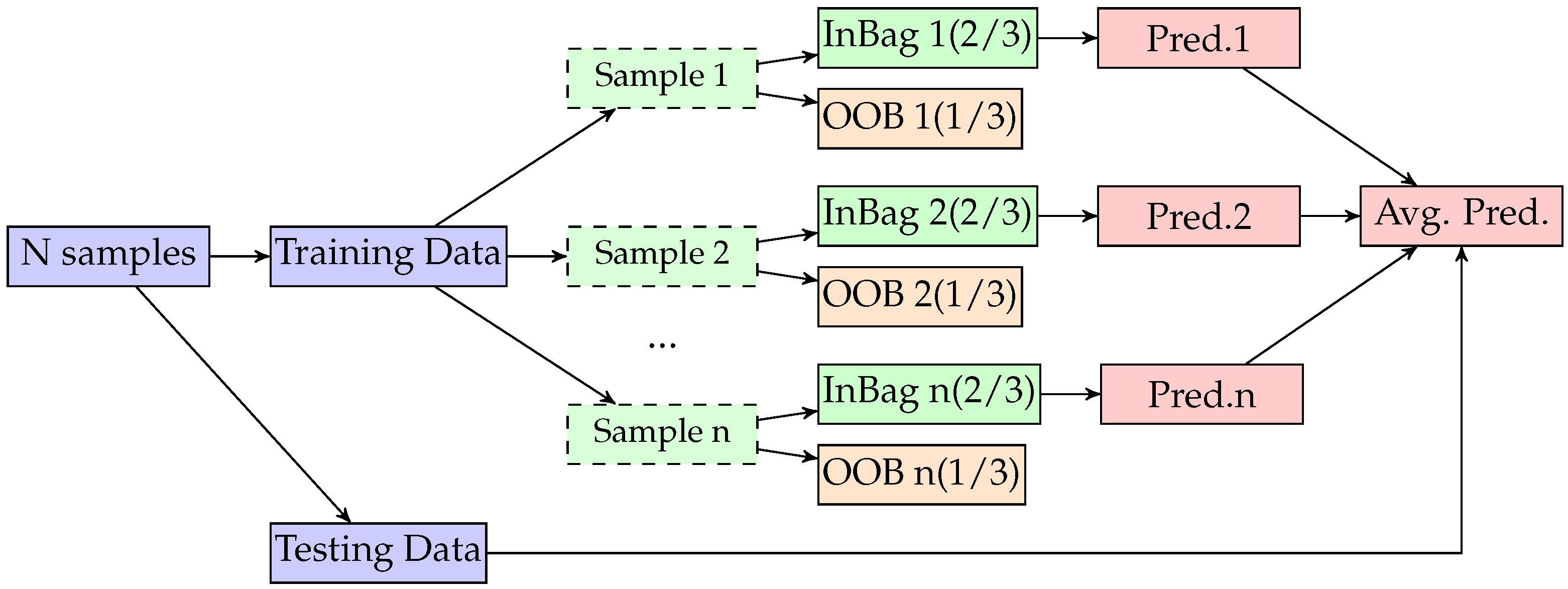
During training, RF constructs multiple decision trees using different subsets of training data generated via bootstrap resampling with replacement. Typically, each bootstrap sample contains roughly two-thirds of the original dataset, while the remaining data, known as out-of-bag (OOB) samples, serves as an internal validation set for estimating generalization error without external cross-validation [34]. This OOB error estimate provides unbiased and computationally efficient model performance insights.
In addition to data perturbation, RF introduces randomness in feature selection at each decision node, considering only a randomly selected subset of available features for determining the optimal split criterion. This random feature subspace method significantly reduces the correlation among trees, thus enhancing model robustness and mitigating overfitting [13,35].
For regression tasks, each tree partitions the input space with the goal of minimizing the mean squared error (MSE) at its leaf nodes. The final RF prediction is obtained by averaging predictions across all N trees:
y ^ ( x ) = 1 N i = 1 N y ^ i ( x ) ,
where y ^ i ( x ) denotes the prediction from the i-th tree.
Due to this dual-randomization and ensemble aggregation strategy, Random Forest consistently exhibits high accuracy, stability, and strong generalization capabilities across diverse application areas [36,37]. In structural engineering and mechanics, RF has found extensive application, including structural reliability analysis [38], damage identification and structural health monitoring (SHM) [39,40], and surrogate modeling of finite element simulation outcomes under nonlinear and high-dimensional conditions [41,42].
In the context of structural analysis, the six surrogate models in our JMA framework (PRS, SVR, RBF, RF, XGB, and LGBM) offer complementary strengths and exhibit distinct limitations. PRS provides a simple and interpretable representation of smooth response surfaces but struggles with sharp discontinuities. SVR is robust to high-dimensional noise and performs well with limited data, yet its training cost increases with dataset size. RBF captures highly nonlinear and smooth trends effectively, though it may scale poorly for large problems. RF can model complex interactions and handle heterogeneous data, but its predictions may lack smoothness and extrapolation capability. XGB and LGBM deliver strong predictive accuracy and handle nonlinear interactions efficiently, but they can be sensitive to noisy or small datasets. The diversity in their modeling characteristics enhances the JMA’s ability to combine their strengths while mitigating individual weaknesses.

4. Methodology

This section presents the surrogate modeling and model averaging framework adopted in this study. We aim to predict the maximum displacement response of a structure under static loading using extracted input features by combining multiple surrogate models via JMA.

4.1. Problem Setup and Base Models

Let { ( x i , y i ) } i = 1 n denote a dataset of n structural simulation instances, where x i R p represents the p-dimensional feature vector derived from the finite element model (e.g., statistics of loading vector b and stiffness matrix A) and y i R is the scalar response variable (e.g., maximum displacement). The prediction task is to learn a function f ^ ( x ) that approximates y from x.
To model the input–output mapping, we employ six surrogate modeling techniques, grouped into two main categories:
  • Classical surrogate models:
    PRS: A second-order global polynomial regression.
    SVR: With radial basis function kernel.
    RBF: Using thin-plate spline basis.
  • Tree-based ensemble models:
    XGB: An efficient implementation of gradient boosting.
    LGBM: Optimized for speed and memory efficiency.
    RF: Ensemble of bagged decision trees with variance reduction.
These two model classes serve as base learners in the proposed JMA framework. Their diversity in model structure and inductive bias provides a strong foundation for building accurate and robust predictive ensembles.

4.2. JMA Framework

Each surrogate model yields a predictor f ^ k ( x ) for k = 1 , 2 , , 6 . Given K base learners, JMA constructs a combined predictor:
f ^ JMA ( x ) = k = 1 K w k f ^ k ( x ) , subject   to   w k 0 ,   k = 1 K w k = 1 ,
where weights { w k } are chosen to minimize the prediction error estimated by cross-validation. In practice, we compute the out-of-fold prediction matrix Z R n × K , where Z i k = f ^ k ( i ) ( x i ) is the prediction of model k on sample i using k-fold CV.
JMA then solves the quadratic program:
min w R K y Z w 2 s . t .   w 0 ,   1 w = 1 .
This approach avoids overfitting and does not require access to the true response on unseen test data.
The complete workflow proceeds as follows:
  • Extract feature vectors x i and response values y i from the simulation data.
  • Train PRS, RBF, and SVR models on a subset of training data.
  • Obtain out-of-fold predictions using k-fold cross-validation and compute JMA weights.
  • Combine the three models using JMA to form the final ensemble predictor.
  • Evaluate the prediction accuracy on a held-out test set.
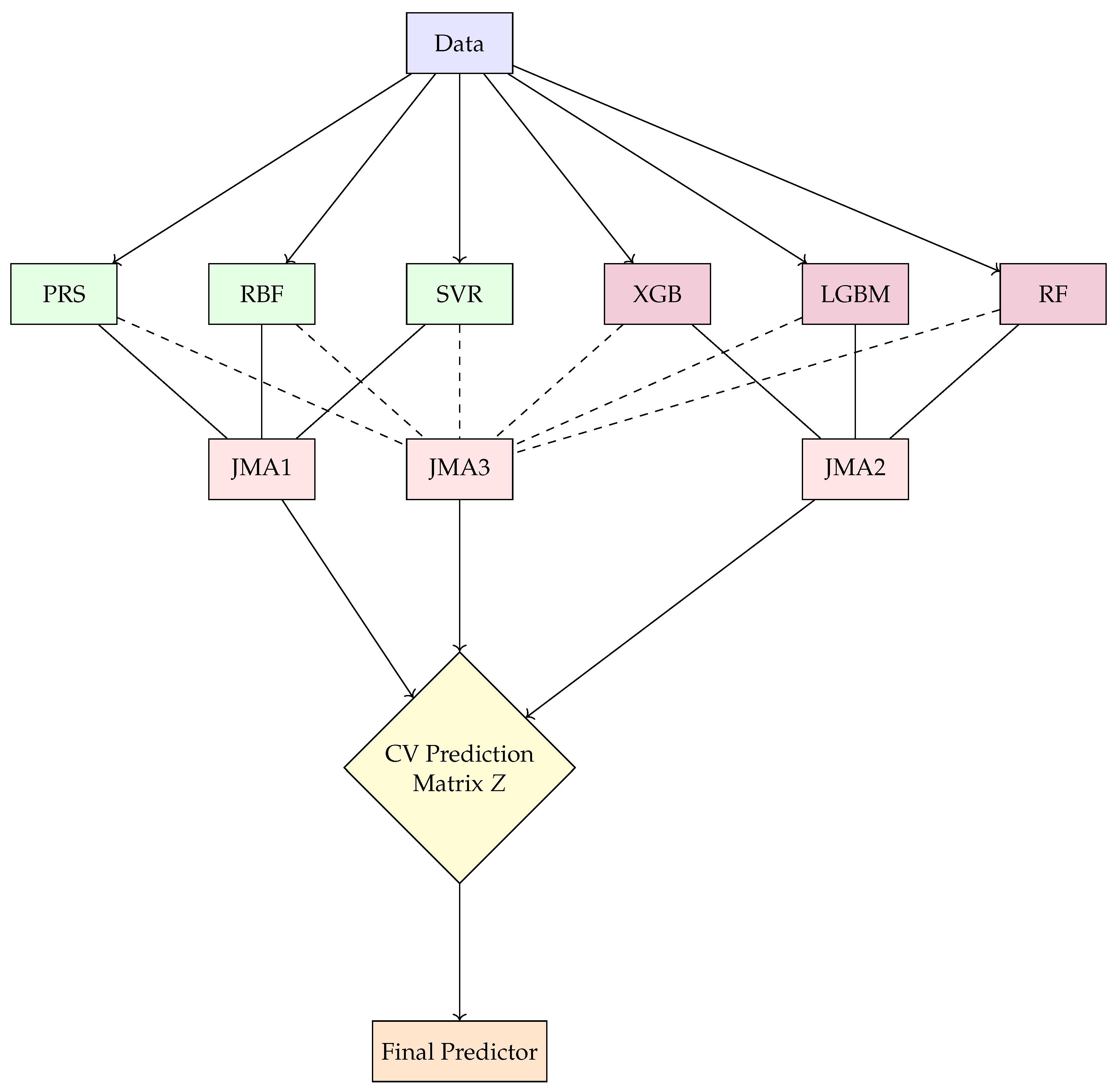
Figure 14 illustrates the overall workflow of the proposed surrogate modeling and model averaging approach. Starting from simulation data, we extract informative features and train three surrogate models: a second-order PRS, an SVR model with an RBF kernel, and an RBF interpolator based on thin-plate splines. For each model, cross-validated predictions are collected to form a prediction matrix. JMA is then applied to compute optimal weights for combining these predictions. The final predictor is evaluated on a separate test set.
The JMA weight estimation procedure is summarized in Algorithm 1. It relies on cross-validated predictions from each surrogate model and solves a constrained quadratic programming problem to derive optimal convex weights.
Algorithm 1 JMA for surrogate modeling
Require: Training data { ( x i , y i ) } i = 1 n , base learners { f ^ k } k = 1 K , number of folds K
Ensure: Final predictor f ^ JMA ( x )
 1: Split data into K folds { D 1 , , D K }
 2: for each base model k = 1 to K do
 3:     for each fold i = 1 to K do
 4:         Train f ^ k ( i ) on D i
 5:         Predict f ^ k ( i ) ( x j ) for all x j D i
 6:     end for
 7:     Collect predictions to form column Z k of matrix Z
 8: end for
 9: Solve the following quadratic program:
min w R K y Z w 2 s . t .   w 0 , 1 w = 1
 10: Form final JMA predictor:
f ^ JMA ( x ) = k = 1 K w k f ^ k ( x )

5. Experiments

This section presents the experimental evaluation of the proposed JMA framework in comparison with individual surrogate models. The goal is to assess the prediction accuracy, robustness, and generalization ability of each approach under repeated subsample training and out-of-distribution testing.

5.1. Experimental Setup

We conduct regression experiments using the stand_small_train subset (100,000 samples) as the training pool and stand_small_test (1000 samples) as the evaluation set. To simulate limited-data conditions and assess model robustness, we randomly sample 2000 training instances without replacement in each repetition.
Each sampled subset is used to fit the following six surrogate models:
  • PRS: Second-order polynomial regression including all pairwise interactions;
  • SVR: SVR with an RBF kernel, implemented via e1071 with default parameters;
  • RBF: Thin-plate spline RBF interpolator trained on the full 2000-sample set;
  • XGB: XGB with 50 boosting rounds and default tree depth;
  • LGBM: LGBM with 50 iterations and default learning rate;
  • RF: RF with 50 trees and depth-limited construction.
In addition to evaluating each model individually, we construct three JMA ensembles:
  • JMA1: Averaging PRS, RBF, and SVR;
  • JMA2: Averaging XGB, LGBM, and RF;
  • JMA3: Averaging all six base models.
For each JMA variant, we estimate out-of-fold predictions using five-fold cross-validation and solve a constrained quadratic program to compute optimal convex weights.
The entire procedure is repeated for 100 independent trials. In each trial, a new 2000-sample subset is drawn, and all models and JMA weights are retrained from scratch. Performance is evaluated on the same 1000 test instances across all repetitions.

5.2. Evaluation Metrics and Experimental Results

5.2.1. Evaluation Metrics

We assess the predictive performance of all surrogate models on the full stand_small_test dataset using three widely adopted regression evaluation metrics: root mean squared error (RMSE), mean absolute error (MAE), and coefficient of determination ( R 2 ). In addition, we include two interval-based metrics derived from conformal prediction (CP), namely the prediction interval coverage rate (CR) and the mean prediction interval width (IW) [43,44,45].
  • RMSE:
    RMSE = 1 n i = 1 n y ^ i y i 2 .
    RMSE measures the magnitude of prediction errors, giving greater weight to larger discrepancies due to the squared term. Thus, it is sensitive to significant deviations and particularly suitable for assessing models where large prediction errors are highly undesirable.
  • MAE:
    MAE = 1 n i = 1 n y ^ i y i .
    MAE quantifies the average absolute prediction error without emphasizing outliers. Compared to RMSE, MAE provides a more balanced representation of a model’s typical prediction accuracy and is less sensitive to extreme observations.
  • R 2 :
    R 2 = 1 i = 1 n y ^ i y i 2 i = 1 n y i y ¯ 2 ,
    where y ¯ denotes the mean of the observed responses. R 2 measures the proportion of variance in the dependent variable explained by the predictive model. A value close to 1 indicates high predictive capability, whereas negative values suggest that the model underperforms compared to a simple mean-based predictor.
  • CP Evaluation Metrics
    To evaluate the predictive uncertainty of each model, we adopt two standard metrics commonly used in the CP literature: CR and IW.
    CR measures the proportion of true response values y i that fall within the predicted confidence interval [ L i , U i ] :
    CR = 1 n i = 1 n I y i [ L i , U i ]
    where I { · } is the indicator function and n is the number of test samples.
    IW quantifies the sharpness of the predicted intervals:
    I W = 1 n i = 1 n ( U i L i )
    A reliable conformal predictor should attain a CR close to the nominal level (e.g., 90%) while maintaining a narrow width W to ensure interval efficiency.
These metrics are computed separately for each of the 100 independent Monte Carlo repetitions and subsequently averaged, ensuring a thorough and robust assessment of the models’ predictive accuracy and generalization capability across different training subsets.

5.2.2. Results and Analysis

Table 1 summarizes the predictive performance of the models across the 100 repetitions, reporting the mean, median, and standard deviation (SD) for RMSE, MAE, and R 2 . It is evident that JMA, particularly JMA1 (combining PRS, RBF, and SVR) and JMA3 (combining all six base models), mostly achieves superior predictive accuracy. Both versions of JMA substantially outperform individual surrogate models, demonstrating the robustness and effectiveness of model averaging in capturing heterogeneous structural response patterns and reducing predictive variability.
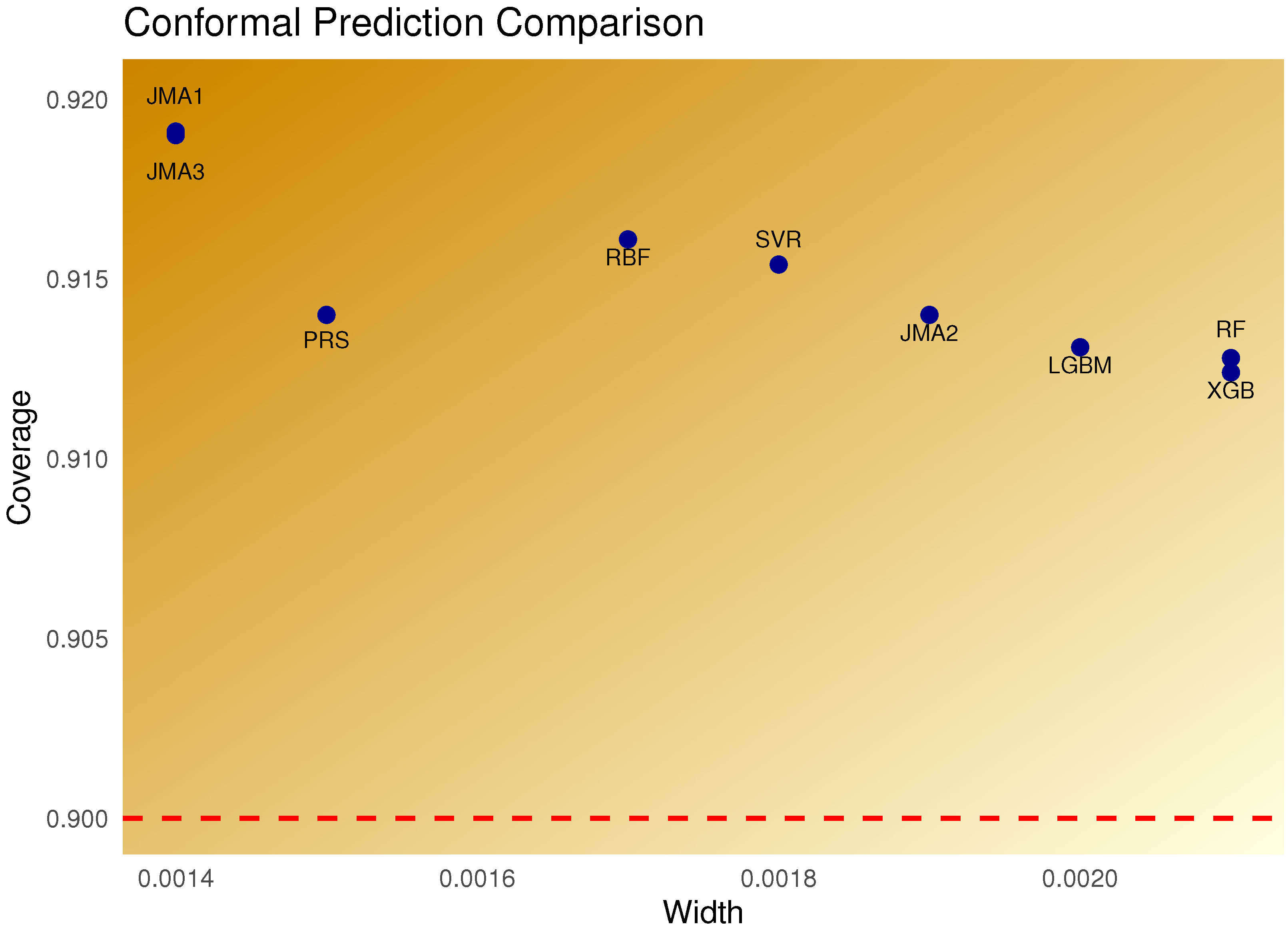
Table 2 summarizes the performance of all models based on their interval coverage and average width at the 90% nominal level. As shown in Table 2, all models achieve CRs slightly above the nominal 90%, indicating the validity of the CP intervals. Among them, JMA1 and JMA3 yield the highest CRs (∼91.9%) while maintaining the narrowest average IW (0.0014), suggesting that these model-averaged predictors strike a superior balance between reliability and precision. In contrast, ensemble tree-based methods like XGB, LGBM, and RF produce relatively wider intervals (around 0.0020–0.0021), which may reflect more conservative uncertainty estimates. SVR and RBF models also perform competitively, with acceptable widths and strong coverage, making them suitable alternatives when computational simplicity is preferred.
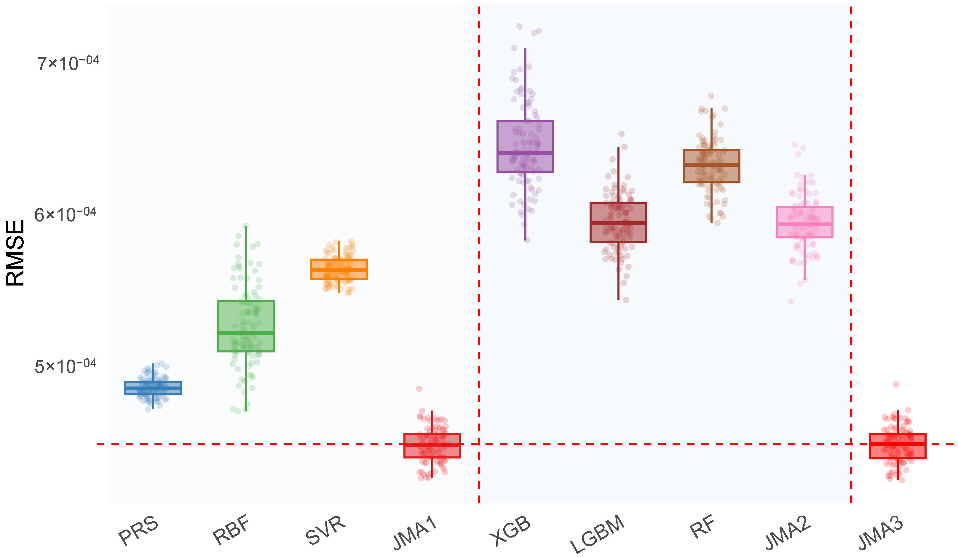
Figure 15 presents the distribution of RMSE values across all repetitions. JMA methods clearly exhibit both a lower median RMSE and reduced variability compared to individual surrogate models. This observation highlights the superior stability and consistency of JMA, particularly JMA1 and JMA3, which effectively leverage the strengths of their respective base models.
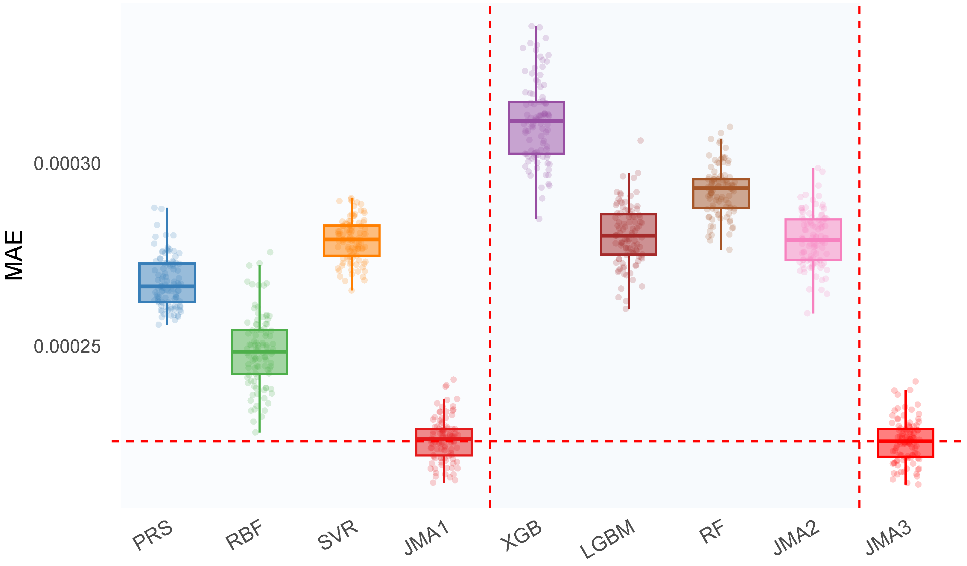
Figure 16 shows the corresponding distributions of MAE. Similar to RMSE, the JMA ensembles (JMA1 and JMA3) demonstrate a significantly lower average MAE and more compact error distributions, further reinforcing their enhanced predictive accuracy and robustness against sampling variability.
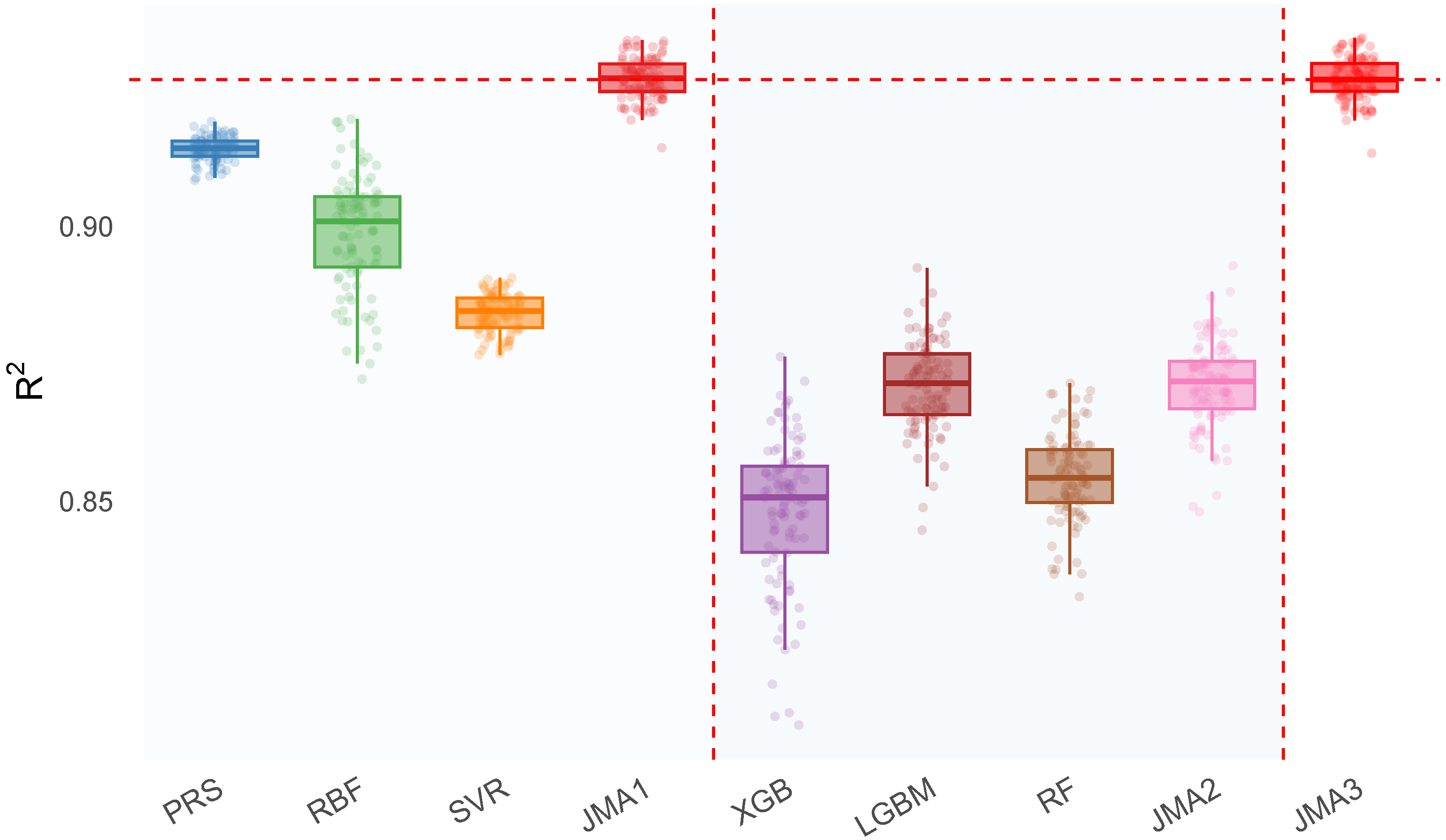
Figure 17 illustrates the distributions of R 2 across the repetitions. The high average R 2 values achieved by JMA methods reflect their strong capability to explain structural response variations, surpassing individual surrogate models by substantial margins.
Finally, Figure 18 illustrates the trade-off between prediction IW and empirical coverage across nine models. The green region (coverage 90 % ) denotes acceptable conformity under the nominal level ( α = 0.1 ), while the red region indicates under-coverage. Models such as JMA1 and JMA3 not only achieve valid coverage but also maintain relatively narrow intervals, highlighting their superior efficiency.
Collectively, these results consistently support the use of model averaging, particularly JMA, as a robust and accurate strategy for surrogate modeling in structural static analyses.

5.3. Summary and Discuss

In summary, our comparative analysis using three widely adopted regression metrics (RMSE, MAE, and R 2 ) clearly demonstrates that the JMA ensemble methods outperform individual surrogate models. JMA1, which integrates classical regression-based approaches, and JMA3, which combines classical and tree-based methods, consistently achieve the lowest prediction errors and the highest R 2 scores. This indicates strong performance and stability across different training samples. These results emphasize the effectiveness of model averaging in improving predictive accuracy and reliability for surrogate modeling in structural static analysis.
While our results show that tree-based models (such as XGB, LGBM, and RF) individually tend to perform less accurately than some classical alternatives on this specific structural dataset, their inclusion remains important. These models are widely used in engineering and scientific computing due to their general robustness, scalability, and ability to handle nonlinear patterns. More importantly, it is difficult to determine a priori which model will perform best for a given dataset. This uncertainty highlights the value of our model averaging approach, which automatically assigns higher weights to better-performing models. As demonstrated in our experiments, this strategy leads to more accurate and stable surrogate predictions, even when some candidate models are suboptimal.
To evaluate the computational cost of JMA relative to its base learners, we recorded the average runtime per iteration for each method across 100 repeated experiments. The results are summarized in Table 3. Simpler models such as PRS and SVR completed training and prediction in under 0.1 s per iteration, whereas more complex models like RBF and ensemble-based methods (e.g., RF, XGB, and LGBM) took moderately longer.
JMA methods (JMA1, JMA2, and JMA3) incurred substantially higher time costs due to the need for cross-validated out-of-fold predictions and solving a constrained quadratic programming problem for weight estimation. JMA3, which aggregates all six candidate models, had the longest average runtime of 31.47 s per iteration. Despite this, the performance gain from JMA, especially in terms of RMSE and R 2 , suggests a worthwhile trade-off between accuracy and computational cost.
Future extensions could consider model screening or adaptive ensemble construction to reduce redundant base learners, thereby improving efficiency while maintaining high predictive accuracy.

6. Conclusions

This paper presents a surrogate modeling framework for static structural analysis based on JMA. We examine the predictive performance of three representative surrogate models: PRS, RBF, and SVR interpolation. These models were selected to capture a range of regression strategies, and their outputs were combined through JMA to exploit their complementary strengths. The proposed framework was evaluated on the StAnD dataset, a large-scale collection of finite element simulations that reflect realistic structural configurations under static loading.
Our experimental results over 100 independent repetitions yield several key observations:
  • JMA consistently outperforms individual surrogate models in terms of RMSE and MAE on held-out test data;
  • The ensemble approach shows greater robustness, characterized by lower prediction variance and the highest number of wins across trials;
  • By leveraging out-of-fold predictions to estimate model weights, JMA remains computationally efficient even in high-dimensional and sparse feature spaces.
These findings demonstrate that model averaging provides an effective and practical strategy for surrogate modeling in structural mechanics, particularly in scenarios where individual models offer varying advantages across different data distributions.
Several avenues remain open for future research. One promising direction is to extend JMA by incorporating more diverse model classes, such as deep neural networks or Gaussian process regressors, which may enhance performance in highly nonlinear settings. Furthermore, integrating additional baseline models commonly used in the field could enrich the comparative analysis and provide a more comprehensive evaluation of the proposed method’s relative strengths. Another direction involves developing adaptive weighting schemes that respond to input-dependent uncertainty and further improve generalization. Additionally, applying this framework to dynamic or nonlinear FEA problems would represent a significant step toward building more versatile surrogate models in computational mechanics.

Author Contributions

Z.Z. contributed to the conceptualization, data collection, and data analysis. N.W. was responsible for drafting and finalizing the manuscript. J.W. provided conceptual input, writing guidance, critical commentary, and revisions. All authors have read and agreed to the published version of the manuscript.

Funding

This research was supported by the Youth Academic Innovation Team Construction project of Capital University of Economics and Business, grant number QNTD202303.

Data Availability Statement

The data presented in this study are available on request from the corresponding author.

Conflicts of Interest

The authors declare no conflicts of interest.

References

  1. Zienkiewicz, O.C.; Taylor, R.L.; Zhu, J.Z. The Finite Element Method: Its Basis and Fundamentals, 6th ed.; Elsevier: Oxford, UK, 2005. [Google Scholar]
  2. Bathe, K.J. Finite Element Procedures; Klaus-Jürgen Bathe: Watertown, MA, USA, 2006. [Google Scholar]
  3. Hadidi, A.; Azar, B.F.; Rafiee, A. Efficient response surface method for high-dimensional structural reliability analysis. Struct. Saf. 2017, 68, 15–27. [Google Scholar] [CrossRef]
  4. Gudipati, V.K.; Cha, E.J. Surrogate modeling for structural response prediction of a building class. Struct. Saf. 2021, 89, 102041. [Google Scholar] [CrossRef]
  5. Ghosh, J.; Padgett, J.E.; Dueñas-Osorio, L. Surrogate modeling and failure surface visualization for efficient seismic vulnerability assessment of highway bridges. Probabilistic Eng. Mech. 2013, 34, 189–199. [Google Scholar] [CrossRef]
  6. Myers, R.H.; Montgomery, D.C.; Anderson-Cook, C.M. Response Surface Methodology: Process and Product Optimization Using Designed Experiments, 3rd ed.; John Wiley & Sons: Hoboken, NJ, USA, 2016. [Google Scholar]
  7. Buhmann, M.D. RBFs: Theory and Implementations; Cambridge University Press: Cambridge, UK, 2003. [Google Scholar]
  8. Ye, J.; Stewart, E.; Zhang, D.; Chen, Q.; Roberts, C. Method for Automatic Railway Track Surface Defect Classification and Evaluation Using a Laser-Based 3D Model. IET Image Process. 2020, 14, 2701–2710. [Google Scholar] [CrossRef]
  9. Drucker, H.; Burges, C.J.C.; Kaufman, L.; Smola, A.; Vapnik, V. SVR Machines. Adv. Neural Inf. Process. Syst. 1997, 9, 155–161. [Google Scholar]
  10. Toh, G.; Park, J. Review of vibration-based structural health monitoring using deep learning. Appl. Sci. 2020, 10, 1680. [Google Scholar] [CrossRef]
  11. Chen, T.; Guestrin, C. XGBoost: A Scalable Tree Boosting System. In Proceedings of the 22nd ACM SIGKDD International Conference on Knowledge Discovery and Data Mining, San Francisco, CA, USA, 13–17 August 2016; Volume 22, pp. 785–794. [Google Scholar] [CrossRef]
  12. Ke, G.; Meng, Q.; Finley, T.; Wang, T.; Chen, W.; Ma, W.; Ye, Q.; Liu, T.-Y. LightGBM: A Highly Efficient Gradient Boosting Decision Tree. Adv. Neural Inf. Process. Syst. 2017, 30, 3146–3154. [Google Scholar]
  13. Breiman, L. Random Forests. Mach. Learn. 2001, 45, 5–32. [Google Scholar] [CrossRef]
  14. Hansen, B.E. Jackknife Model averaging, asymptotic risk, and minimax efficiency. J. Econom. 2012, 167, 52–67. [Google Scholar] [CrossRef]
  15. Lu, X.; Su, L. Jackknife model averaging for quantile regressions. J. Econom. 2015, 188, 40–58. [Google Scholar] [CrossRef]
  16. Cheung, Y.-W.; Wang, W. A jackknife model averaging analysis of RMB misalignment estimates. J. Int. Commer. Econ. Policy 2020, 11, 2050007. [Google Scholar] [CrossRef]
  17. Zhang, X.; Zou, G.; Wan, A.T. Model averaging by jackknife criterion in models with dependent data. J. Econom. 2013, 174, 82–94. [Google Scholar] [CrossRef]
  18. Ando, T.; Li, K.-C. A model-averaging approach for high-dimensional regression. J. Am. Stat. Assoc. 2014, 109, 254–265. [Google Scholar] [CrossRef]
  19. You, K.; Wang, M.; Zou, G. Jackknife model averaging for composite quantile regression. J. Syst. Sci. Complex. 2024, 37, 1604–1637. [Google Scholar] [CrossRef]
  20. He, B.; Ma, S.; Zhang, X.; Zhu, L.-X. Rank-based greedy model averaging for high-dimensional survival data. J. Am. Stat. Assoc. 2023, 118, 2658–2670. [Google Scholar] [CrossRef]
  21. Grementieri, L.; Finelli, F. StAnD: A Dataset of Linear Static Analysis Problems. arXiv 2022, arXiv:2201.05356. [Google Scholar] [CrossRef]
  22. Box, G.E.P.; Wilson, K.B. On the Experimental Attainment of Optimum Conditions. J. R. Stat. Soc. Ser. B (Methodol.) 1951, 13, 1–45. [Google Scholar] [CrossRef]
  23. Dackermann, U.; Smith, W.A.; Randall, R.B. Damage identification based on response-only measurements using cepstrum analysis and artificial neural networks. Struct. Health Monit. 2014, 13, 430–444. [Google Scholar] [CrossRef]
  24. Cheng, K.; Lu, Z. Adaptive Bayesian SVR model for structural reliability analysis. Reliab. Eng. Syst. Saf. 2021, 206, 107286. [Google Scholar] [CrossRef]
  25. Kazemi, F.; Çiftçioğlu, A.Ö.; Shafighfard, T.; Asgarkhani, N.; Jankowski, R. RAGN-R: A multi-subject ensemble machine-learning method for estimating mechanical properties of advanced structural materials. Comput. Struct. 2025, 308, 107657. [Google Scholar] [CrossRef]
  26. Yang, J.; Hao, Y.; Peng, D.; Shi, J.; Zhang, Y. Machine learning-based methods for predicting the structural damage and failure mode of RC slabs under blast loading. Buildings 2025, 15, 1221. [Google Scholar] [CrossRef]
  27. Li, S.; Jin, N.; Dogani, A.; Yang, Y.; Zhang, M.; Gu, X. Enhancing LightGBM for industrial fault warning: An innovative hybrid algorithm. Processes 2024, 12, 221. [Google Scholar] [CrossRef]
  28. Aslam, F. Advancing Credit Card Fraud Detection: A Review of Machine Learning Algorithms and the Power of Light Gradient Boosting. Am. J. Comput. Sci. Technol. 2024, 7, 9–12. [Google Scholar] [CrossRef]
  29. Prajisha, C.; Vasudevan, A.R. An efficient intrusion detection system for MQTT-IoT using enhanced chaotic salp swarm algorithm and LightGBM. Int. J. Inf. Secur. 2022, 21, 1263–1282. [Google Scholar] [CrossRef]
  30. Wang, D.-N.; Li, L.; Zhao, D. Corporate finance risk prediction based on LightGBM. Inf. Sci. 2022, 602, 259–268. [Google Scholar] [CrossRef]
  31. Zhang, D.; Gong, Y. The Comparison of LightGBM and XGBoost Coupling Factor Analysis and Prediagnosis of Acute Liver Failure. IEEE Access 2020, 8, 220990–221003. [Google Scholar] [CrossRef]
  32. Ho, T.K. Random decision forests. In Proceedings of the 3rd International Conference on Document Analysis and Recognition (ICDAR’95), Montreal, QC, Canada, 14–16 August 1995; IEEE: Piscataway, NJ, USA, 1995; pp. 278–282. [Google Scholar]
  33. Breiman, L.; Friedman, J.H.; Olshen, R.A.; Stone, C.J. Classification and Regression Trees; Chapman & Hall/CRC: Boca Raton, FL, USA, 1984. [Google Scholar]
  34. Liaw, A.; Wiener, M. Classification and Regression by randomForest. R News 2002, 2, 18–22. [Google Scholar]
  35. Hastie, T.; Tibshirani, R.; Friedman, J. The Elements of Statistical Learning: Data Mining, Inference, and Prediction, 2nd ed.; Springer: Berlin/Heidelberg, Germany, 2009. [Google Scholar] [CrossRef]
  36. Fernández-Delgado, M.; Cernadas, E.; Barro, S.; Amorim, D. Do We Need Hundreds of Classifiers to Solve Real-World Classification Problems? J. Mach. Learn. Res. 2014, 15, 3133–3181. [Google Scholar]
  37. Ziegler, A.; König, I.R. Mining Data with Random Forests: Current Options for Real-World Applications. WIREs Data Min. Knowl. Discov. 2014, 4, 55–63. [Google Scholar] [CrossRef]
  38. Vatani, A.; Jafari-Asl, J.; Ohadi, S.; Safaeian Hamzehkolaei, N.; Afzali Ahmadabadi, S.; Correia, J.A.F.O. An Efficient Surrogate Model for Reliability Analysis of the Marine Structure Piles. Proc. Inst. Civ. Eng.-Marit. Eng. 2023, 176, 176–192. [Google Scholar] [CrossRef]
  39. Zhou, Q.; Ning, Y.; Zhou, Q.; Luo, L.; Lei, J. Structural Damage Detection Method Based on Random Forests and Data Fusion. Struct. Health Monit. 2013, 12, 48–58. [Google Scholar] [CrossRef]
  40. Lei, X.; Sun, L.; Xia, Y.; He, T. Vibration-Based Seismic Damage States Evaluation for Regional Concrete Beam Bridges Using Random Forest Method. Sustainability 2020, 12, 5106. [Google Scholar] [CrossRef]
  41. Trinchero, R.; Larbi, M.; Torun, H.M.; Canavero, F.G.; Swaminathan, M. Machine Learning and Uncertainty Quantification for Surrogate Models of Integrated Devices with a Large Number of Parameters. IEEE Access 2018, 7, 4056–4066. [Google Scholar] [CrossRef]
  42. Esteghamati, M.Z.; Flint, M.M. Developing Data-Driven Surrogate Models for Holistic Performance-Based Assessment of Mid-Rise RC Frame Buildings at Early Design. Eng. Struct. 2021, 245, 112971. [Google Scholar] [CrossRef]
  43. Vovk, V.; Gammerman, A.; Shafer, G. Algorithmic Learning in a Random World; Springer: Berlin/Heidelberg, Germany, 2005. [Google Scholar]
  44. Shafer, G.; Vovk, V. A tutorial on conformal prediction. J. Mach. Learn. Res. 2008, 9, 371–421. [Google Scholar]
  45. Borrotti, M. Quantifying Uncertainty with Conformal Prediction for Heating and Cooling Load Forecasting in Building Performance Simulation. Energies 2024, 17, 4348. [Google Scholar] [CrossRef]
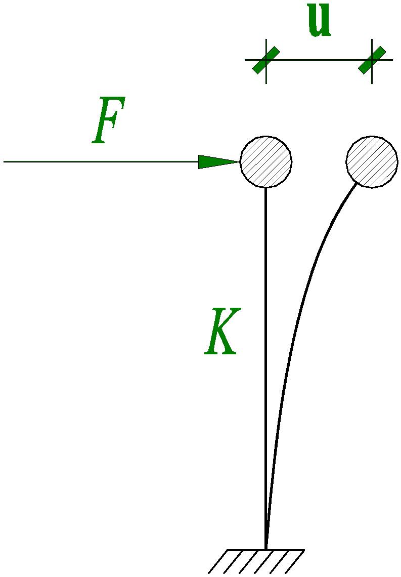
Figure 1. Illustration of lateral deformation in a single-story frame subjected to a horizontal load F. The frame, modeled with an equivalent lateral stiffness K, undergoes a horizontal displacement u . The curved shape indicates shear-induced deformation of the structure under horizontal load.
Buildings 15 02872 g001
Figure 2. A regular three-dimensional frame structure composed of uniformly distributed vertical and horizontal members, representing a typical small-scale model with consistent height and cross-section.
Buildings 15 02872 g002
Figure 3. A stepped-height frame structure generated by removing a random number of upper-level units, resulting in a compact model with moderate geometric complexity and reduced overall height.
Buildings 15 02872 g003
Figure 4. An irregular frame structure featuring multiple height reductions and asymmetrical geometry, representing a large-scale configuration with significant variation in spatial distribution and structural topology.
Buildings 15 02872 g004
Figure 5. Schematic diagram of slab load transfer from a uniformly distributed load to supporting beams using triangular and trapezoidal distribution patterns. The uniformly distributed slab load q is idealized as being directed toward the midpoints of the supporting beams at a 45 angle, indicating the assumed load paths for structural modeling.
Buildings 15 02872 g005
Figure 6. Equivalent uniform load on supporting beams resulting from slab dead load and live load. The uniformly distributed slab load q is converted into equivalent uniform loads: q l / 4 on short-span beams and q l ( L l / 2 ) / ( 2 L ) on long-span beams, where L and l denote the long and short slab spans, respectively.
Buildings 15 02872 g006
Figure 7. Boxplots of six structural features and the response variable in the training dataset.
Buildings 15 02872 g007
Figure 8. Workflow for constructing and applying PRS models. Overview of the surrogate-based optimization procedure consisting of four stages: problem formulation, data preparation, modeling, and optimization.
Buildings 15 02872 g008
Figure 9. Illustration of RBF surrogate interpolation. Black dots represent sample points from simulation or experiment. Each blue dashed curve corresponds to an RBF centered at a sampled location. The red solid curve represents the RBF surrogate obtained by summing these basis functions with appropriate weights.
Buildings 15 02872 g009
Figure 10. Comparison of SVR with a linear kernel (a) and a nonlinear RBF kernel (b). The ε -insensitive tube is shown as dashed lines; filled points are within the tube and open circles are outside.
Buildings 15 02872 g010
Figure 11. Illustration of the XGBoost algorithm. The model sequentially builds additive decision trees f t ( X , θ t ) , where each tree is trained to approximate the negative gradient L ( t ) of a specified loss function L , representing the residuals at iteration t. The final prediction F ( X ) is an ensemble of the outputs from all individual trees. Additionally, a complexity regularization term Ω ( f ) = γ T + 1 2 λ j w j 2 is introduced to penalize the number of leaves T and the magnitude of leaf weights w j , thereby controlling overfitting.
Buildings 15 02872 g011
Figure 12. Illustration of the LGBM workflow. The algorithm processes input data by applying GOSS, feature binning (histogram construction), and EFB for continuous variables and optimal categorical split for discrete features. A leaf-wise growth strategy is used to construct decision trees by maximizing gain, and the final prediction is the sum of all trees in the ensemble.
Buildings 15 02872 g012
Figure 13. Illustration of the Random Forest training process. Each tree is trained on a bootstrap sample (InBag), and predictions are made independently. The final output is obtained by aggregating individual predictions. OOB samples are used for internal error estimation.
Buildings 15 02872 g013
Figure 14. Layered workflow with centralized data node, six base learners, and three JMA strategies.
Buildings 15 02872 g014
Figure 15. Boxplots of RMSE across 100 independent repetitions for each surrogate model. The horizontal dashed line corresponds to the median of the optimal method, and the vertical dashed line is used only to distinguish method categories.
Buildings 15 02872 g015
Figure 16. Boxplots of MAE across 100 independent repetitions for each surrogate model. The horizontal dashed line corresponds to the median of the optimal method, and the vertical dashed line is used only to distinguish method categories.
Buildings 15 02872 g016
Figure 17. Boxplots of R 2 across 100 independent repetitions for each surrogate model. The horizontal dashed line corresponds to the median of the optimal method, and the vertical dashed line is used only to distinguish method categories.
Buildings 15 02872 g017
Figure 18. Scatter plot of coverage vs. width (CP trade-off plot). The horizontal dashed line represents the true confidence level.
Buildings 15 02872 g018
Table 1. Performance summary: mean, median, and SD for RMSE, MAE, and R 2 . (Best mean values indicated in bold.) All RMSE and MAE values are scaled by 10 3 .
MethodRMSE ( × 10 3 )MAE ( × 10 3 ) R 2
MeanMedianSDMeanMedianSDMeanMedianSD
PRS0.4860.4850.0060.2670.2660.0070.9140.9140.002
RBF0.5260.5210.0270.2490.2480.0100.9000.9010.010
SVR0.5640.5630.0080.2790.2790.0060.8840.8850.003
JMA10.4480.4480.0110.2250.2250.0060.9270.9270.004
XGB0.6450.6460.0290.3110.3120.0110.8480.8510.014
LGBM0.5950.5940.0190.2800.2800.0080.8710.8720.008
RF0.6330.6330.0170.2930.2930.0070.8540.8540.008
JMA20.5950.5940.0180.2790.2790.0070.8710.8710.008
JMA30.4480.4480.0120.2240.2240.0060.9270.9270.004
Table 2. Evaluation of 90% prediction intervals using split CP. (Best mean values indicated in bold.)
ModelCRIW
PRS0.91400.0015
RBF0.91610.0017
SVR0.91540.0018
XGB0.91240.0021
LGBM0.91310.0020
RF0.91280.0021
JMA10.91900.0014
JMA20.91400.0019
JMA30.91910.0014
Note: Theprediction IWs are relatively small due to the low magnitude of the response variable in this dataset.
Table 3. Average computation time per iteration (in seconds).
MethodPRSSVRRBFJMA1XGBLGBMRFJMA2JMA3
Time (s)0.0020.08110.18330.6020.0340.0210.2231.38831.466
Disclaimer/Publisher’s Note: The statements, opinions and data contained in all publications are solely those of the individual author(s) and contributor(s) and not of MDPI and/or the editor(s). MDPI and/or the editor(s) disclaim responsibility for any injury to people or property resulting from any ideas, methods, instructions or products referred to in the content.