Evaluation of Optimum Thermal Insulation for Mass Walls in Severe Solar Climates of Northern Chile

Abstract

The Life Cycle Cost Assessment (LCCA) methodology is widely used to determine the optimal thickness of thermal insulation for walls and roofs. The results depend on several factors, such as the degree day calculations method, the ambient or sol–air temperature, base temperature variations, and the heat capacity of the thermal envelope elements. This study aims to analyze the impact of solar radiation on mass walls with different orientations in five cities in northern Chile, which have severe solar climates. The goal is to determine the optimal thickness of expanded polystyrene insulation using the LCCA method, considering solar radiation, a varying base temperature, and validating results by analyzing the energy demand for heating and cooling of a typical house. The findings show that excluding solar radiation in the LCCA methodology can lead to an underestimation of the optimal insulation thickness by 21–39% for walls in northern Chile. It was also found that using variable monthly threshold temperatures for heating and cooling based on the adaptive thermal comfort model results in a slight underestimation (1–3%) of the optimal thickness compared to a constant annual temperature. An energy simulation of a typical house in five cities in northern Chile showed that neglecting the effect of solar radiation when determining the thermal insulation thickness for the studied wall can lead to a minor increase in heating and cooling energy demand, ranging from approximately 1% to 9%. However, this study emphasizes the importance of applying optimal insulation thickness for cities with more continental climates like Santiago and Calama, where the heating demand is higher than cooling.

1. Introduction

In the 21st century, climate change is a critical challenge, intensified by the high environmental impact of traditional construction [1,2]. Given this reality, it is crucial for the construction industry to evolve toward more sustainable practices. The search for sustainable alternatives in construction presents itself as a critical solution to reduce environmental impact [3]. It is not merely about carrying out construction projects but doing so in a way that promotes harmony between societal development and the environment.

The increasing energy demand, exacerbated by the depletion of fossil resources and climate change, necessitates a more efficient and effective use of energy in residential and commercial buildings, industrial construction sectors, transportation, and service industries [4].

In recent years, there has been a considerable increase in energy consumption in buildings due to various factors, including climate change, population growth, and the pursuit of improved living conditions in general [5]. A significant portion of the energy consumed in buildings is allocated to heating and cooling loads, which can account for around 30% of a country’s total consumption [6]. These thermal loads are largely attributed to heat loss or gain through the building envelope. Reducing heat transfer through the envelope can effectively decrease the energy consumption in buildings. In this context, a passive and highly effective method to reduce environmental loads is to apply thermal insulation to the external walls of the building. However, it is important to consider that increasing the thickness of the insulation reduces the heat transfer load but also raises the installation cost [7]. Therefore, it is essential to determine the optimum thickness that minimizes the total cost for insulation and HVAC energy use of the building throughout its lifecycle [8], especially considering the impact of climate change and the future rise in temperatures.

Associated with the above, there are various alternative solutions, such as energy optimization methods through simulations, where iterative processes can be used to optimize various components of any type of building related to its energy efficiency, economic optimization, and ecological impact [9,10]. The selection of the optimal insulation thickness is crucial, as excessive insulation may not justify its additional cost and could even be counterproductive in certain climates by increasing the cooling load [11,12]. The main optimization methodologies include energy modeling and simulation using software such as DesignBuilder (which uses EnergyPlus), TRNSYS, Dest, or IDA ICE, which allow simulation of the building’s energy performance [11,13]. These simulations consider variables such as building orientation, window-to-wall ratio (WWR), internal heat gains, and material properties, enabling the identification of the optimal thermal insulation for the building envelope. To optimize the results of multiple simulations, algorithms such as non-dominated sorting genetic algorithm II (NSGA II), genetic algorithms (GAs), or particle swarm optimization (PSO) are commonly used [11,14]. These algorithms, often coupled with energy simulations and artificial neural networks (ANNs), aim to minimize multiple objectives simultaneously, such as energy consumption and cost, among others [13].

Another approach to determine the optimal thickness of thermal insulation is the use of analytical methods, which involve solving heat transfer equations across the building envelope. For example, the finite difference method and Fourier transform techniques are commonly used to solve these equations under steady or periodic conditions [15,16].

A complementary approach is Life Cycle Assessment (LCA), an essential methodology to evaluate the total environmental impact of construction materials and systems throughout the entire life cycle of a building—from production to end-of-life. Considering the embodied carbon of materials is increasingly important, as materials with higher embodied carbon may not be offset by lower operational energy consumption [15,17].

Another approach is the Life Cycle Cost Analysis (LCCA) method, a widely used and proven methodology globally, which serves as a useful tool for economic evaluation that contributes to achieving sustainable goals, attaining long-term performance by improving operational costs in buildings [18]. This approach goes beyond merely considering the initial costs and also evaluates the long-term implications. The main aim of LCCA is to balance the economic and environmental impact. By assessing the direct and indirect costs associated with a project, from raw material extraction to the eventual demolition of the structure, it provides a more comprehensive perspective. This holistic approach enables construction professionals to make informed decisions that benefit both economic profitability and environmental sustainability.

A concrete example of applying LCCA is in precisely the determination of the optimum thickness of insulation in walls [19,20,21]. Instead of automatically opting for the most cost-effective solution in the short term, LCCA considers energy costs over time, as well as the environmental impact associated with energy consumption. This can lead to the choice of a thicker insulation which, although initially more expensive, results in significant savings over the building’s lifecycle, as well as a reduction in carbon emissions. Generally, the alternative that presents the lowest total cost over its life cycle is considered the most economical and, therefore, may be the preferred option [22]. The recent research presents 47 examples of studies defining the optimum thermal insulation thickness for walls using the LCCA methodology, highlighting the scientific interest in this method from various research institutions worldwide, demonstrating its suitability for different types of walls and thermal insulation applications [23]. Furthermore, the authors of the study [21] emphasize the importance of considering solar radiation for warmer regions of the world, particularly those with extreme solar climates due to their proximity to the equator. This parameter is crucial, and the need to include it in the LCCA methodology to determine the optimum insulation thickness is discussed [21,24]. Considering the effect of solar radiation to correct degree days tends to be a complicated task due to the number of meteorological and geographical factors in the building’s location [4]. Therefore, it is necessary to take into account both the different orientations of the studied wall and the corresponding hourly variations in global solar radiation for each orientation [25]. Solar radiation directly impacts the exterior walls, generating a thermal load that must be controlled by the thermal insulation system [26]. The intensity of solar radiation, local climatic conditions, and seasonal variations are key factors that impact the amount of heat to be mitigated. Heat transfer through walls is responsible for 20–40% of the cooling load for different buildings in various climatic zones [27]. In regions with high temperatures and prolonged sun exposure, more effective insulation is required to reduce unwanted heat gain.

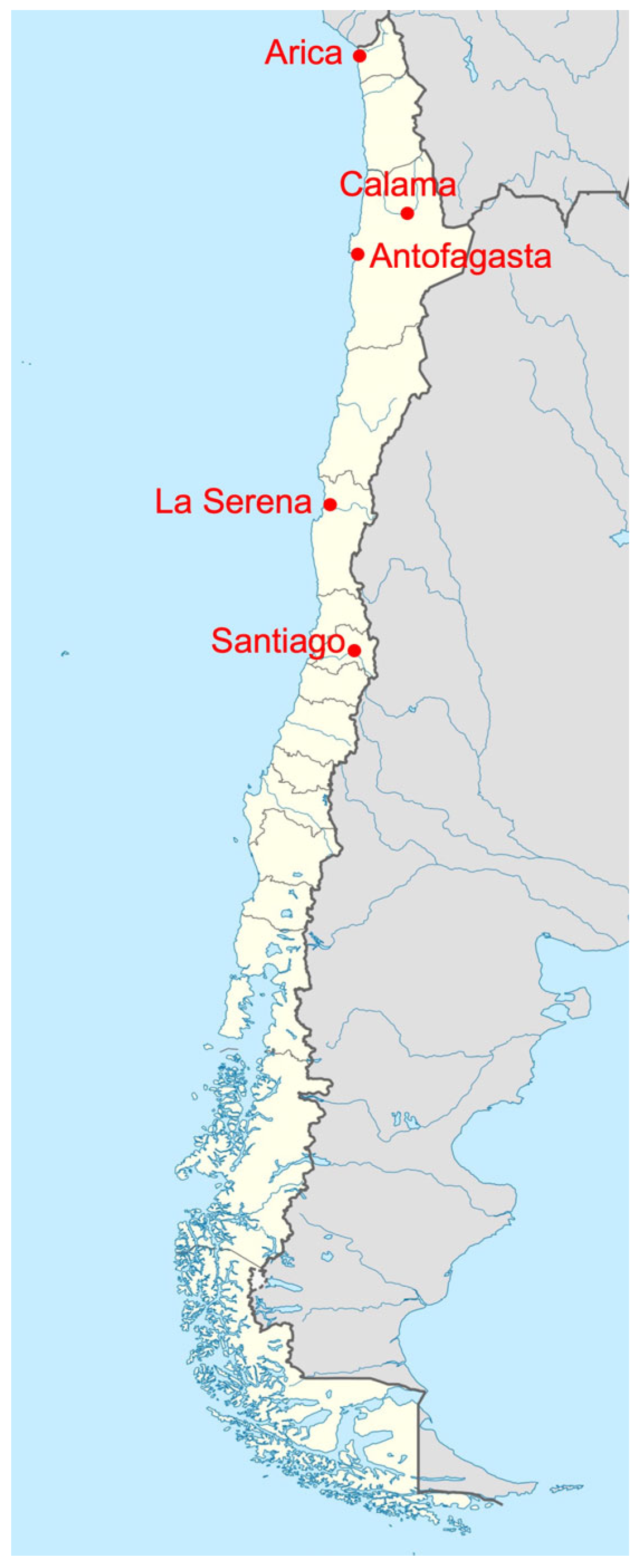
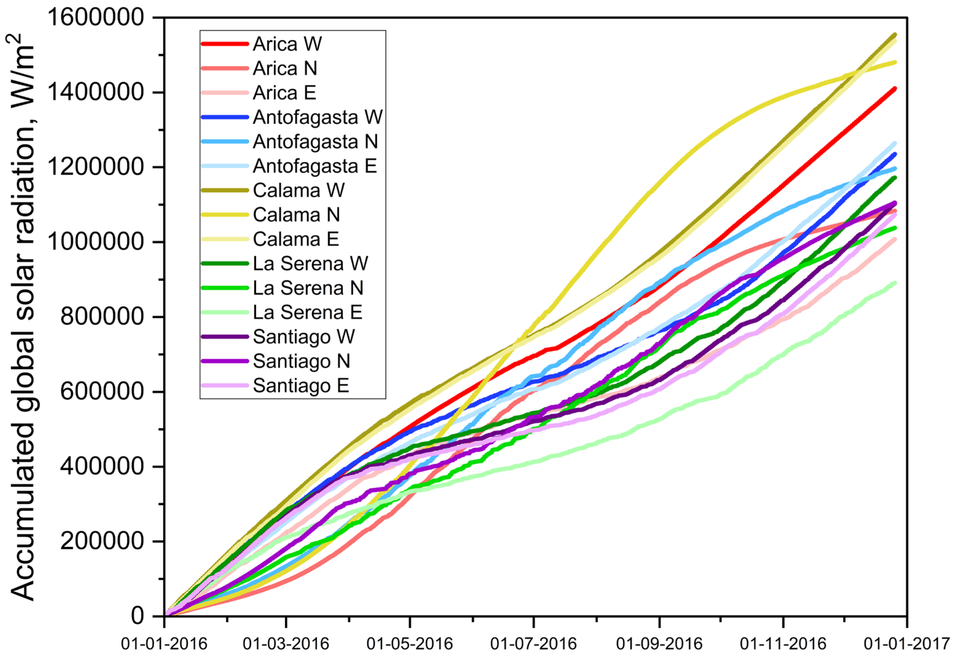
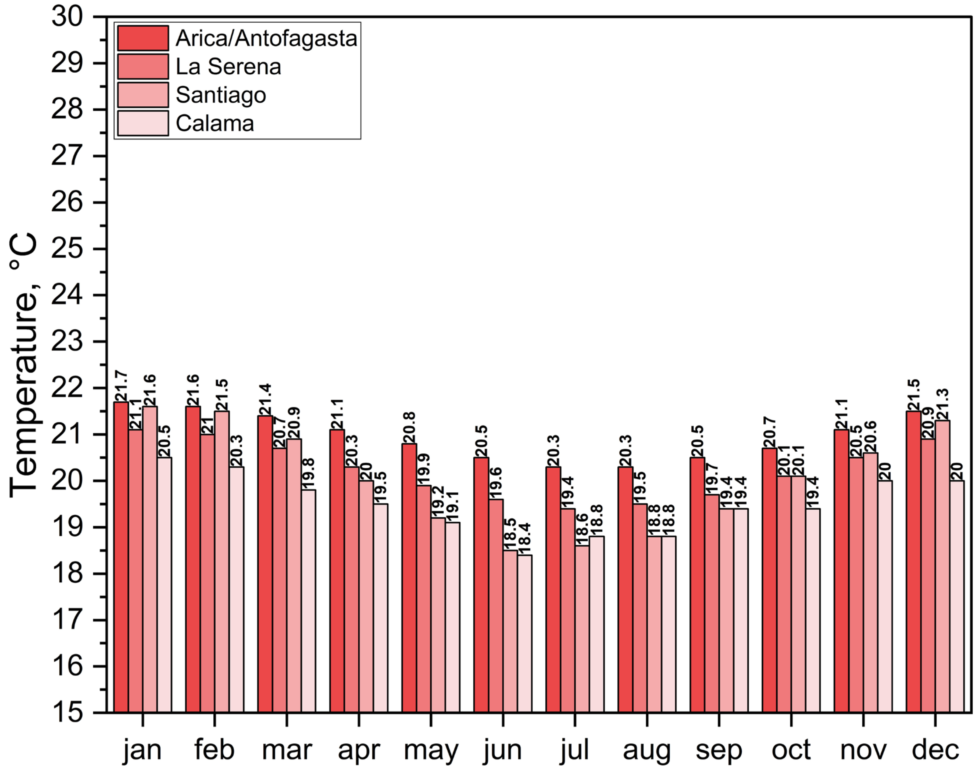
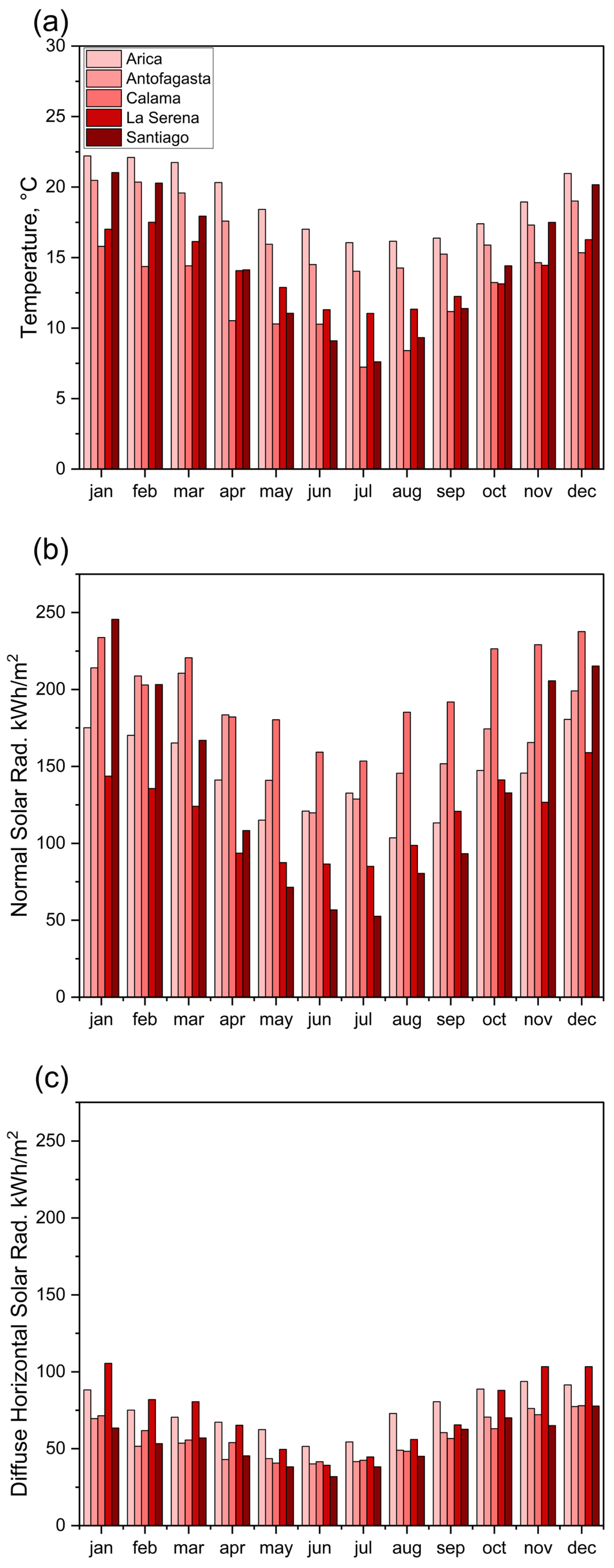
One of the countries characterized by an extremely solar climate is Chile, specifically in the north of the country, where the annual average values of global horizontal solar radiation can reach up to 2400–2800 kWh/m² [28].

The design of thermal envelope elements for buildings in Chile is based on national construction regulations that set maximum permissible values for thermal transmittance (U) in different geographical locations [29,30]. However, these regulations do not consider various local geophysical and geographical aspects [31]. Therefore, it is essential to determine the optimum insulation thickness, which in turn will allow the determination of an optimum U-value for the thermal envelope elements of buildings using the LCCA methodology. This approach is a suitable alternative for customized project designs in different geographical zones of Chile.

When using the LCCA methodology to define the optimum thickness of thermal insulation for walls in northern Chile, it is necessary to determine the influence of solar radiation, as this can significantly affect the determination of the optimum insulation thickness in these extremely hot areas [32] for mass walls and its effect on the energy demand for heating and cooling of a typical house in the area. In this context, the main objective of this research will be to analyze the necessity of considering solar radiation in the calculation of the optimum thermal insulation thickness for mass walls through the LCCA methodology in the cities of northern Chile.

2. Materials and Methods

The methodology begins with a geographical description of the study area, specifying the cities analyzed. Next, the process for obtaining meteorological data is detailed. This is followed by an explanation of the wall construction solution under analysis. Finally, the LCCA methodology is presented.

2.1. Study Area: Cities in the North of Chile

The study area consists of five cities in northern Chile, selected for their population relevance and geographical location associated with the solar radiation they receive. These cities, from north to south, are Arica, Calama, Antofagasta, La Serena, and Santiago.

Arica and Antofagasta, located in the extreme north, exhibit hot desert climates, characterized by high temperatures and scarce precipitation. Calama shares similar conditions but is situated away from the coastal zone. Meanwhile, La Serena experiences a semi-arid climate with dry and mild seasons. Finally, Santiago, the capital, has a Mediterranean climate with hot, dry summers contrasting with cooler, wetter winters [32]. Figure 1 presents a map of the northern part of the country, highlighting the geographical locations of the cities.

2.2. Global Solar Radiation and Ambient Temperature Data

Global solar radiation corresponds to the sum of direct radiation, diffuse radiation, and ground-reflected radiation. To obtain this parameter for each of the five study cities, the Solar Explorer tool was used [33,34]. This tool provides meteorological data for the entire territory of Chile with a spatial resolution of 90 meters and a temporal resolution of 1 h for the period between 2004 and 2016.

For each city, a central point was selected (

Table 1. Geographic coordinates of locations studied in each city.

City	Lat. [°]	Lon. [°]	Alt. [m]
Arica	−18.4777	−70.3135	0
Calama	−22.4527	−68.9259	2269
Antofagasta	−23.6517	−70.3976	19
La Serena	−29.9098	−71.2585	10
Santiago	−33.4465	−70.6606	550

), and data on global solar radiation for walls with a 90° inclination and for north, east, and west orientations were extracted, along with the ambient temperature data for the year 2016, with a temporal resolution of 1 h. For the south orientation, ambient temperature data in the shade were used.

Figure 2 presents a graph showing the sum of hourly values of solar radiation incident on the study wall with different orientations in the study cities throughout the year. The most significant difference in accumulated global solar radiation for the three main orientations was observed in the cities of La Serena and Arica. In Antofagasta, the maximum solar radiation was observed for the east-facing wall orientation. All these differences are related to the orography of the geographical points selected for this study. The city of Calama is characterized by the highest sums of accumulated global solar radiation throughout the year for three wall orientations, due to its inland location. In the case of coastal cities, cloudy weather conditions are observed in the morning on some days of the year, which is why the minimum solar radiation is characteristic, for example, of La Serena.

In the case of ambient temperature, Figure 3 presents statistical box-plot graphs of hourly temperature data for the year 2016 in the study cities. The annual average temperatures are characteristic of the northern cities—Arica and Antofagasta. Meanwhile, La Serena is characterized by the lowest annual average temperature. Santiago and Calama, on the other hand, are characterized by a marked thermal amplitude, due to continentality and altitude effects. In any case, positive temperatures are observed throughout the year in all cities, with the exception of Calama, where temperatures can drop below 0 °C for a few days.

The data from the year 2016 was chosen because at the time of this study, it was the latest year available in the Solar Explorer. It was considered that one year was sufficiently representative for the objectives set in the present research.

2.3. Studied Wall Construction Solution

The construction solution used to determine the optimum thermal insulation thickness was the one proposed in [21] which has already been previously used and validated in other works [35,36].

Figure 4 shows the composition of the wall for which the necessary thermal resistance for subsequent calculations was obtained, and

Table 2. Components of the construction solution for the studied wall for optimizing the optimum thickness of thermal insulation.

Layer	Title of Layer	Thickness	Thermal Conductivity	Thermal Resistance
		[m]	[W/mK]	[m2K/W]
	Indoor air thermal resistance			0.13
1	High-strength plaster	0.02	0.56	0.036
2	hollow brick	0.05	0.445	0.112
3	EPS	x	0.034
4	Cement or lime mortar	0.025	1.3	0.019
5	Perforated brick	0.115	0.991	0.116
6	Cement or lime mortar	0.025	1.3	0.019
	Outside air thermal resistance			0.04

details the thermal properties of the studied wall. Various layers were included, such as high-strength plaster, hollow brick, expanded polystyrene (EPS) with variable thickness (x), cement or lime mortar, and perforated brick. The thermal resistances of the interior and exterior air were also considered. The thermal resistance of the analyzed wall without considering the thermal insulation is 0.472 m²K/W.

2.4. Optimum Thickness Determination

In this section, the methodology for calculating degree days will be presented first, followed by the LCCA methodology.

2.4.1. Calculation of Heating and Cooling Degree Days

To determine the optimum thermal insulation thickness, it is necessary to know the indicators that allow the evaluation of energy demand per square meter of exchange with the exterior. For greater precision, the simultaneous effect of two indicators was considered: cooling degree days (CDD) using Equation (1) and heating degree days (HDD) using Equation (2) of the “hourly” method [37].

$$CDD={\displaystyle \frac{1}{24}}{\sum }_h({\theta }_{sa}-{\theta }_c{)}_j^{+};$$

(1)

$$HDD={\displaystyle \frac{1}{24}}{\sum }_h({\theta }_h-{\theta }_{sa}{)}_j^{+};$$

(2)

where ${\theta }_{sa}$ is the sol–air temperature, the calculation of which is detailed in Equation (3). The threshold temperatures for cooling—${\theta }_c$, and for heating—${\theta }_h$ were considered variable for each month of the year according to the thermal zone of each city, as per the Sustainable Construction Standards for Housing, Volume II: Energy (ECS) [38] (Figure 5 and Figure 6).

Figure 5 presents the recommended monthly threshold temperatures (or interior temperatures) for heating in the study cities, and Figure 6 presents the recommended temperatures for cooling. These were determined based on the adaptive comfort method outlined in ASHRAE Handbook Fundamentals, chapter “Thermal Comfort” [39].

The heating temperature threshold corresponds to +2.5 °C above the adaptive comfort temperature, while the cooling threshold corresponds to −2.5 °C below it, according to the methodology proposed by de Dear and Brager [40]. This temperature range defines the 90% acceptability band for adaptive thermal comfort in the general population. These thresholds depend on the monthly average outdoor temperatures of the building climate zones where the studied cities are located; therefore, the comfort temperatures vary between cities.

The temperatures in Figure 5 and Figure 6 were used to calculate the annual values of HDDs and CDDs, respectively. The cities of Arica and Antofagasta are located in the same building climate zone; hence, they have the same threshold temperatures for heating and cooling. These temperatures represent the thermal comfort limits at which the heating or cooling system is expected to be activated, as appropriate. Additionally, they are variable because the range of comfort temperatures shifts due to the thermal adaptation of individuals and the climatic conditions of each city. To analyze the effect that variable temperatures can have on the optimum thickness, calculations were also performed considering fixed threshold temperatures for each city using an average for thermal comfort, as shown in

Table 3. Annual average threshold temperatures for heating and cooling.

Climate Zone	${\mathit{\theta }}_{\mathit{h}}$, [°C]	${\mathit{\theta }}_{\mathit{c}}$, [°C]
A (Arica, Antofagasta)	20.90	26.02
C (La Serena)	20.33	25.18
D (Santiago)	20.16	25.20
H (Calama)	19.62	24.52

, with average values from Figure 5 and Figure 6 for each city.

The climate zones considered for each city were those recommended by ECS and can be seen in Table 3. It is important to note that for Calama, the recommendation to use zone H was followed. In the ECS climate zoning, the zones range from warmer to colder, starting from letter A [30].

For the calculation of the sol–air temperature, the same procedure was followed as in in study [24], using Equation (3).

$${\theta }_{sa}={\theta }_0+{\displaystyle \frac{\alpha }{h_0}}{I}_t-{\displaystyle \frac{\epsilon \sigma \left({\theta }_0^4-{\theta }_{sur}^4\right)}{h_0}};$$

(3)

where ${\theta }_0$ is the outdoor air temperature provided by the Solar Explorer in K; $I_t$ is the hourly global solar radiation provided by the Solar Explorer for each wall orientation; $\alpha$ is the absorptivity of the exterior material, which for this study was considered to be 0.55, equivalent to a greyish exterior coating; $h_0$ is the combined heat transfer coefficient for convection and radiation on the wall, with a value of 20 $\mathrm{W}/{\mathrm{m}}^2\mathrm{K}$ based on Chilean standard NCh853 [41]; $\mathsf{\epsilon }$ is the exterior material surface emissivity taken as 0.9; $\mathsf{\sigma }$ is the Stefan–Boltzmann constant in ${\displaystyle \frac{\mathrm{W}}{{\mathrm{m}}^2{\mathrm{K}}^4}};$ and ${\theta }_{sur}$ is the temperature of the sky and surrounding surfaces in K calculated with Equation (4).

$${\theta }_{sur}=\sqrt[4]{{\epsilon }_{air}{ \ast \theta }_o^4};$$

(4)

where ${\epsilon }_{air}$ is the thermal emittance of the air, and ${\theta }_0$ is the outdoor air temperature provided by the Solar Explorer. It should be noted that there are different empirical equations for estimating the thermal emittance of air, which depend on various meteorological parameters [42,43,44]. For this study, a value of 0.75 was used.

Additionally, the annual values of HDDs and CDDs were calculated according to Equations (1) and (2) using the ambient temperature, i.e., with variable base temperatures (Figure 5 and Figure 6) and with constant annual values (Table 3).

2.4.2. LCCA Methodology

In this study, only the costs of insulation and the costs associated with the operation of heating and cooling systems were considered, as performed in [20,21,45], which in turn were based on [19,46].

To derive the expression that allowed for the determination of the optimum thermal insulation thickness, it was considered that the heat loss per unit area (square meter) of exchange with the exterior is defined as in Equation (5).

$$q_w=U_w·∆T;$$

(5)

where $∆T$ is the difference between the indoor and outdoor temperatures, which will later be replaced by the heating and cooling degree days, and $U_w$ is the thermal transmittance of the wall. Then, the heat loss or gain are converted to annual energy demand by multiplying $q_w$ by HDDs or CDDs and by 86,400 s and dividing by 3.6 × 10⁶, resulting in units of kWh for heating, Equation (6), and for cooling, Equation (7).

$${ED}_{heat}=0.024{\displaystyle \frac{HDD}{R_{wall}}};$$

(6)

$${ED}_{cool}=0.024{\displaystyle \frac{CDD}{R_{wall}}};$$

(7)

where HDDs and CDDs are the annual values of heating and cooling degree days, and $R_{wall}$ is the thermal resistance of the wall in ${\mathrm{m}}^2\mathrm{K}/\mathrm{W}$.

Heat transfer in this study is calculated using a static method, meaning the time-dependent partial differential equation for thermal conduction is not solved. This approach is considered acceptable, as demonstrated in the study by [47], where the Heating Degree Days (HDDs) method was compared with a dynamic simulation and yielded similar results

Then, the energy consumption cost associated with m² of wall is defined as in Equations (8) and (9).

$${EC}_{heat}=0.024{\displaystyle \frac{HDD·C_{elec}}{R_{wall}·\eta }};$$

(8)

$${EC}_{cool}=0.024{\displaystyle \frac{CDD·C_{elec}}{R_{wall}·\epsilon }};$$

(9)

where $C_{elec}$ is the cost of electricity in USD per kWh, as detailed in

Table 4. Cost of electricity for the cities under study.

City	[USD/kWh]
Arica	0.11
Antofagasta	0.11
Calama	0.10
La Serena	0.12
Santiago	0.12

, $\eta$ is the SCOP, with a value of 2.5 for the cooling of the electric air conditioning system in this study; $\epsilon$ is the SEER of the heating, with a value of 3.0. Thus, the costs per m² for heating and cooling were defined as in Equation (10) and Equation (11), respectively, by multiplying the above by the Present Worth Factor (PWF), defined in Equation (15).

$${EC}_{heat}=0.024{\displaystyle \frac{HDD·C_{elec}·PWF}{R_{wall}^{actual}·\eta }};$$

(10)

$${EC}_{cool}=0.024{\displaystyle \frac{CDD·C_{elec}·PWF}{R_{wall}^{actual}·\epsilon }};$$

(11)

where $R_{wall}^{actual}$ is the thermal resistance of the wall in m²K/W without considering the thermal insulation. Subsequently, the costs for heating and cooling for the optimized wall were defined by Equations (12) and (13).

$${EC}_{heat}=0.024{\displaystyle \frac{HDD·C_{elec}·PWF}{{(R}_{wall}^{actual}+\frac{x}{\lambda })·\eta }};$$

(12)

$${EC}_{cool}=0.024{\displaystyle \frac{CDD·C_{elec}·PWF}{(R_{wall}^{actual}+\frac{x}{\lambda })·\epsilon }};$$

(13)

where x is the thickness of the insulation in meters and $\lambda$ is the conductivity of the EPS, taken as 0.034 W/mK for this study. Finally, the total cost will be the sum of the cooling cost, the heating cost, and the insulation cost. From this relationship, it is possible to define the thickness variable, as was achieved in [21], and it is defined in Equation (14). This thickness was calculated for the four main orientations in each city.

$$x_{heat-cool,wall}^{opt}={\left(0.024{\displaystyle \frac{HDD·C_{elec}·PWF·\lambda }{C_{insu}·\eta }}+0.024{\displaystyle \frac{CDD·C_{elec}·PWF·\lambda }{C_{insu}·\epsilon }}\right)}^{1/2}-R_{wall}^{actual}·\lambda ;$$

(14)

where $C_{insu}$ is the cost per m³ of insulation in USD. PWF is an economic factor necessary for the optimization of energy costs, and it is defined in Equation (15).

$$PWF=\left\{\begin{array}{c}{\displaystyle \frac{(1+r{)}^N-1}{(1+r{)}^N·r}}, when i\ne g\\ {\displaystyle \frac{N}{(1+i)}}, when i=g\end{array}\right.;$$

(15)

where $N$ is the expected useful lifetime; $i$ is the interest rate; and $r$ is defined by Equation (16).

$$r=\left\{\begin{array}{c}{\displaystyle \frac{i-g}{1+g}}, when i>g\\ {\displaystyle \frac{g-i}{1+i}}, when i<g\end{array}\right.;$$

(16)

where g is the inflation rate.

For this study, economic data from the past 20 years were considered, as referenced in [48], as shown in

Table 5. Inflation and interest rates for the past 20 years in Chile according to information from the Central Bank of Chile.

Average for the Period 2004–2023
Inflation rate	Interest rate
3.90%	3.99%

.

Using the data from Table 5 and an expected useful lifetime of (N = 30) years, a PWF of 29.6 was obtained.

For the cost of thermal insulation, various sources were consulted, and it was determined that the price of 43.65 USD/m³ shown in [49] is sufficiently representative of the national market value of the EPS. On the other hand, the cost of electricity for each city was based on [50,51], using the tariff corresponding to single-phase low voltage lines. The consumption values of electricity for each city are presented in Table 4. The date of consultation of prices for both thermal insulation and the cost of electricity was 29 August 2024.

2.4.3. Validation of Optimum Thermal Insulation Thicknesses Using Energy Simulation

To validate the results of the optimum thicknesses obtained through the LCCA methodology, an energy demand analysis for cooling and heating of a typical house in northern Chile will be implemented using DesignBuilder—Energy Plus. The optimum EPS thickness values, both considering and not considering solar radiation, will be applied to the exterior walls of the house presented in Figure 7. This house is two-story; its northward orientation can be observed in Figure 7. The main characteristics of this house are presented in

Table 6. Summary of the building specifications.

Parameters	Value
Total floor area	68.4 m2
Floor with soil contact	30.4 m2
External wall area	127.1 m2
Roof	34.9 m2
Ceiling height	2.5 m
Total window area	15.6 m2
Total door area	1.5 m2

.

Table 7. Thermal transmittance values of the thermal envelope elements.

Ceiling–Roof Assembly
	e, [m]	λ, [W/mK]	R, [m2K/W]
Rse			0.04
Zinc roofing	0.0005	110.00	0.00
Waterproof felt	0.0003		0.01
OSB 650 kg/m3	0.009	0.13	0.07
Air	0.2		0.15
Glass wool 20 kg/m3	0.1	0.036	2.78
Gypsum Plasterboard 900 kg/m3	0.01	0.25	0.04
Rsi			0.10
		R total value, [m2K/W]	3.19
		U total value, [W/m2K]	0.31
Glazing
	e, [m]	λ, [W/mK]	R, [m2K/W]
Rse			0.04
Exterior glass	0.006	0.90	0.01
Air	0.013		0.19
Interior glass	0.006	0.90	0.01
Rsi			0.13
		R total value, [m2K/W]	0.37
		U total value, [W/m2K]	2.68
Floor on the ground
	e, [m]	λ, [W/mK]	R, [m2K/W]
Rsi			0.17
Ceramic/clay tiles	0.01	0.80	0.01
Cast concrete	0.07	1.13	0.06
Polyethyline HD	0.001	0.50	0.00
Sand and gravel	0.19	2.00	0.10
Rse			0.04
		R total value, [m2K/W]	0.38
		U total value, [W/m2K]	2.62
Exterior flooring (2-nd floor)
	e, [m]	λ, [W/mK]	R, [m2K/W]
Rsi			0.17
Timber flooring	0.005	0.14	0.04
Glass wool 20 kg/m3	0.1	0.036	2.78
Gypsum Plasterboard 900 kg/m3	0.01	0.25	0.04
Rse			0.04
		R total value, [m2K/W]	3.06
		U total value, [W/m2K]	0.33

presents the materials that make up the construction solutions of the house’s thermal envelope and the calculated thermal transmittance values. It should be noted that the house’s second floor has exterior flooring with a U-value of 0.33 W/m²K. The windows consist of two 6 mm glass panes with a 13 mm air gap. The windows and exterior door have a 4 cm wooden frame with a U-value of 2.63 W/m²K. The entrance door is made of 3.5 cm wood with a U-value of 2.82 W/m²K.

The walls were simulated using the information presented in Table 2, varying only the thicknesses of the EPS thermal insulation based on the results obtained by applying the LCCA methodology to define the optimum thickness in previous stages of the methodology. For the studied wall, it was decided to analyze the heat capacity (or specific heat) using Equation (17).

$$\chi ={\displaystyle \frac{\sum {\rho }_i{C}_i{e}_i}{1000}};$$

(17)

where ${\rho }_i$—density of the material of layer i of the building element, kg/m³; $C_i$—specific heat capacity of the material of layer i of the building element, J/kgK; and $e_i$—thickness of layer i of the building element, m. According to the Sustainable Construction Standards of Chile (ECS) [38], the heat capacity value $\chi$ (kJ/m²K) defines whether a wall is “light” with $\chi$ < 70 kJ/m²K; “medium” with $\chi$ between 70 and 200 kJ/m²K; and “heavy” with $\chi$ > 200 kJ/m²K.

Table 8. Heat capacity of the studied wall without considering thermal insulation.

Material	e, m	${\mathit{C}}_{\mathit{i}}$, [J/kgK]	${\mathit{\rho }}_{\mathit{i}}$, [kg/m3]	${\mathit{\chi }}_{\mathit{i}}$, [J/m2K]
High-strength plaster	0.02	1300	1350	35,100
Hollow brick	0.05	840	1000	42,000
Cement or lime mortar	0.025	940	1900	44,650
Perforated brick	0.115	880	2170	219,604
Cement or lime mortar	0.025	940	1900	44,650
			$\chi$, [kJ/m2K]	386.0

presents the results of the χ calculation for the studied wall without considering thermal insulation. The specific heat capacity values for the materials were taken from the same ECS document. According to the ECS classification, this wall is “heavy” and has high heat capacity. According to ASHRAE Standard 90.1, this wall is classified as a “mass wall” [52].

It should be noted that for the energy simulation, the effect of thermal bridges has been neglected. Other simulation parameters include occupancy. The occupancy of this house was 0.03 persons/m². Heat gain per person is taken as 130 W. The occupancy schedule is as follows:

For weekdays: Until 05:00, 0.5; Until 10:00, 1.0; Until 15:00, 0.5; Until 24:00, 1.0.

For weekends: Until 07:00, 0.5; Until 21:00, 1.0; Until 24:00, 0.5.

Heat gain from equipment per m² of floor area is taken as 1.57 W. Heat gain from lighting per m² of floor area is taken as 2.5 W. The lighting schedule is as follows:

For weekdays: Until 07:00, 0.0; Until 10:00, 1.0; Until 17:00, 0.0; Until 24:00, 1.0.

For weekends: Until 09:00, 0.0; Until 21:00, 1.0; Until 24:00, 0.0.

Heating and cooling setpoint temperatures were taken as constant throughout the year and for each city according to Table 3.

To perform the energy simulation, the epw meteorological files of the five studied cities were applied. Figure 8 presents the monthly average values of ambient temperature (a), the monthly average values of normal solar radiation (b), and the diffuse horizontal solar radiation (c). Differences in these parameters among the five cities are notable, but the ranges of these parameters are adequate, and the temporal distribution is consistent with the general climatic conditions of each city.

3. Results and Discussion

The results section is divided into three parts. The first part considers variable threshold temperatures for cooling and heating (θc and θh), presenting the optimum thicknesses obtained using the LCCA method with the sol–air temperature (θsa), taking into account the effect of solar radiation, and the method using ambient temperature (θo), which does not consider it. The second part of the results presents an analysis of the same parameters, but with constant cooling and heating thresholds throughout the year for each city. In the third part, the results of the validation of the optimum thicknesses are presented alongside the results of the energy demand simulation in the study cities for a typical house in the study area.

3.1. Optimum Thermal Insulation Thicknesses for Variable Threshold Temperatures

Table 9. Optimum thermal insulation thicknesses for variable ${\theta }_h$ and ${\theta }_c$.

City	Temp.	Orientation	ΣCDDs	ΣHDDs	x, [cm]
Arica	θsa	W	1088.7	588.6	17.5
Arica	θsa	N	714.8	582.4	15.4
Arica	θsa	E	700.4	589.0	15.3
Arica	θo	S	9.1	708.4	11.6
Calama	θsa	W	678.9	1010.9	25.2
Calama	θsa	N	558.7	981.0	23.8
Calama	θsa	E	687.2	997.0	22.9
Calama	θo	S	0.0	1299.9	19.9
Antofagasta	θsa	W	1520.8	1961.8	17.7
Antofagasta	θsa	N	1272.5	1860.9	16.9
Antofagasta	θsa	E	1145.4	1752.2	17.6
Antofagasta	θo	S	42.5	2050.9	15.9
La Serena	θsa	W	667.4	1570.0	22.1
La Serena	θsa	N	460.9	1532.8	20.9
La Serena	θsa	E	339.3	1527.8	20.3
La Serena	θo	S	1.3	1879.6	20.7
Santiago	θsa	W	1034.0	1603.8	23.7
Santiago	θsa	N	921.7	1537.0	22.9
Santiago	θsa	E	822.4	1504.5	22.3
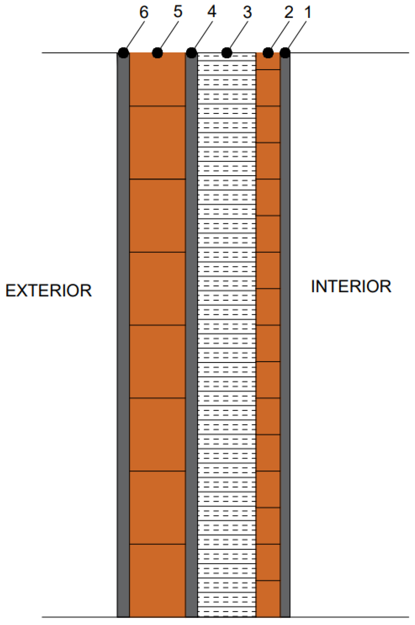
Santiago	θo	S	119.2	1765.5	20.4

presents the results of the optimum thickness (x) obtained for each city, method, and orientation of the studied wall, along with the annual sums of CDDs and HDD. A notable difference can be observed between the annual values of CDDs based on sol–air temperature compared to CDDs based on ambient temperature in all the cities studied. The west orientation in all cities is characterized by having the maximum CDDs θsa. Due to the orographic aspects of Chile, the presence of the high Andes mountains in the eastern part of the country influences the modelling of global solar radiation. As in the Northern Hemisphere, in summer, the east and west facades receive more radiation than the south facades [53], which is why the CDDs θsa of the west wall is greater than that of the south wall. Furthermore, the solar radiation simulation takes into account the hourly variable effect of cloud cover [34], which influences the final CDDs results calculated based on sol–air temperature. The values of CDDs θo are almost negligible, as the cooling limit thresholds were developed based on the adaptive thermal comfort model.

In the case of HDDs, considering the effect of solar radiation on average decreases the annual value of HDD θo by 16% in all cities for three orientations, with a minimum decrease in the city of Calama. This result is logical due to the transition to θsa considering solar gains. The variation in HDD θsa by orientation is not as notable in almost all cities (Table 9).

Regarding the optimum thicknesses of EPS thermal insulation for the analyzed wall construction solution (Table 9), the greatest differences between optimum thicknesses were identified in Arica and Calama when comparing those that considered solar radiation and those that did not. In Antofagasta, the optimum insulation thickness considering the effect of solar radiation was on average 1.5 cm greater than the optimum thickness based on degree days calculated with ambient temperature. In Santiago, this difference reached 2.6 cm, and in La Serena, a minimum of 0.4 cm was observed (

Table 10. Average optimum thicknesses for variable ${\theta }_h$ and ${\theta }_c$.

City	${\overline{\mathit{x}}}_{\mathit{\theta }\mathit{s}\mathit{a}}^{\mathit{v}\mathit{a}\mathit{r}}$, [cm]	${\overline{\mathit{x}}}_{\mathit{\theta }\mathit{o}}^{\mathit{v}\mathit{a}\mathit{r}}$, [cm]	Δ, [cm]	Δ, [%]
Arica	16.1	11.6	4.5	39%
Calama	24.0	19.9	4.1	21%
Antofagasta	17.4	15.9	1.5	9%
La Serena	21.1	20.7	0.4	2%
Santiago	23.0	20.4	2.6	11%

). The highest value of optimum thickness for the west orientation of the wall is related to the specific characteristics of the solar climate in Chile, which were previously mentioned, explaining the differences in the degree day results. Therefore, the effect of considering solar radiation is notable in the LCCA methodology for calculating the optimum thickness of thermal insulation in different geographical locations.

Table 10 presents the results of the average optimum thickness for three orientations exposed to solar radiation and for the south orientation, which was taken as the ambient temperature (θo). In this way, an optimum thickness of thermal insulation was obtained for each city, considering the effect of solar radiation in some cases and not in others.

Table 10 details the final optimum thicknesses using variable threshold temperatures for the case where solar radiation is considered—average value by three orientations (${\overline{x}}_{\mathsf{\theta }\mathrm{s}\mathrm{a}}^{var})$ and the case where it is ignored (${\overline{x}}_{\mathsf{\theta }\mathrm{o}}^{var})$. Additionally, Δ denotes the difference between methods, either absolute or percentage.

From Table 10, it can be observed that the greatest variations in optimum thickness between methods occurred in Arica, with 39%, and to a lesser extent in Calama, with 21%. In both cases, the absolute thickness variations exceeded 4 cm. For the rest of the cities studied, the influence was considerably smaller, especially in La Serena, where there was only a 2% increase. This underscores the importance of considering the sol–air temperature when defining the optimum wall insulation thicknesses using the LCCA method for Arica and Calama, due to their more severe solar regime compared to other cities. The same recommendation should be applied to other regions of the world that have a climate similar to these cities.

3.2. Optimum Thicknesses of Thermal Insulation for Constant Threshold Temperatures

Table 11. Optimum thermal insulation thicknesses for constant ${\theta }_h$ and ${\theta }_c$.

City	Temp.	Orientation	ΣCDD	ΣHDD	${\mathit{x}}^{\mathit{c}\mathit{t}\mathit{e}}$, [cm]
Arica	θsa	W	1098.2	606.4	17.7
Arica	θsa	N	714.9	599.5	15.5
Arica	θsa	E	718.2	611.8	15.6
Arica	θo	S	16.7	744.7	12.0
Calama	θsa	W	1531.0	2003.2	25.4
Calama	θsa	N	1268.1	1893.5	24.0
Calama	θsa	E	1157.7	1788.4	23.1
Calama	θo	S	55.1	2098.5	20.2
Antofagasta	θsa	W	690.4	1018.3	17.8
Antofagasta	θsa	N	554.1	980.8	16.8
Antofagasta	θsa	E	695.0	1002.7	17.7
Antofagasta	θo	S	0.0	1306.0	15.9
La Serena	θsa	W	687.9	1623.9	22.5
La Serena	θsa	N	470.9	1578.0	21.2
La Serena	θsa	E	359.1	1583.5	20.7
La Serena	θo	S	1.5	1935.8	21.0
Santiago	θsa	W	1067.8	1692.4	24.3
Santiago	θsa	N	943.7	1615.6	23.4
Santiago	θsa	E	870.0	1596.2	23.0
Santiago	θo	S	154.3	1869.4	21.2

includes the result of the optimum thickness, denoted by x^cte, for the case where the threshold temperatures are constant in each city, considering the heating and cooling limits indicated in Table 3.

Table 11 highlights the low thicknesses in Arica and Antofagasta using the θo temperature, which is attributed to the low sums of CDDs and HDDs. Additionally, it is important to mention that in general, the obtained thicknesses were slightly higher compared to those that considered the effect of solar radiation.

Table 12. Average optimum thicknesses for constant ${\theta }_h$ and ${\theta }_c$.

City	${\overline{\mathit{x}}}_{\mathit{\theta }\mathit{s}\mathit{a}}^{\mathit{c}\mathit{t}\mathit{e}}$, [cm]	${\overline{\mathit{x}}}_{\mathit{\theta }\mathit{o}}^{\mathit{c}\mathit{t}\mathit{e}}$	Δ, [cm]	Δ, [%]
Arica	16.3	12.0	4.3	36%
Calama	24.1	20.2	3.9	19%
Antofagasta	17.4	15.9	1.5	9%
La Serena	21.5	21.0	0.5	2%
Santiago	23.6	21.2	2.4	11%

details the final thicknesses using constant threshold temperatures, differentiating between the case that considers solar radiation—average value by three orientations (${\overline{x}}_{\mathsf{\theta }\mathrm{s}\mathrm{a}}^{cte})$ and the case that ignores it (${\overline{x}}_{\mathsf{\theta }\mathrm{o}}^{cte})$. Additionally, Δ denotes the difference between methods, either in absolute or percentage terms.

From Table 12, it can be observed that the use of constant threshold temperatures slightly increases the average optimum thicknesses of thermal insulation in all study cases. Additionally, the percentage variations are quite similar to those obtained with variable threshold temperatures.

It is important to note that the use of constant temperatures simplifies the calculations but may underestimate or overestimate the actual heating and cooling needs due to the absence of seasonal variations. This can result in significant differences in insulation thickness, especially in extreme climates. On the other hand, variable threshold temperatures, adjusted monthly according to the ECS methodology, provide a more accurate and adapted representation of real conditions, improving the precision of the analysis.

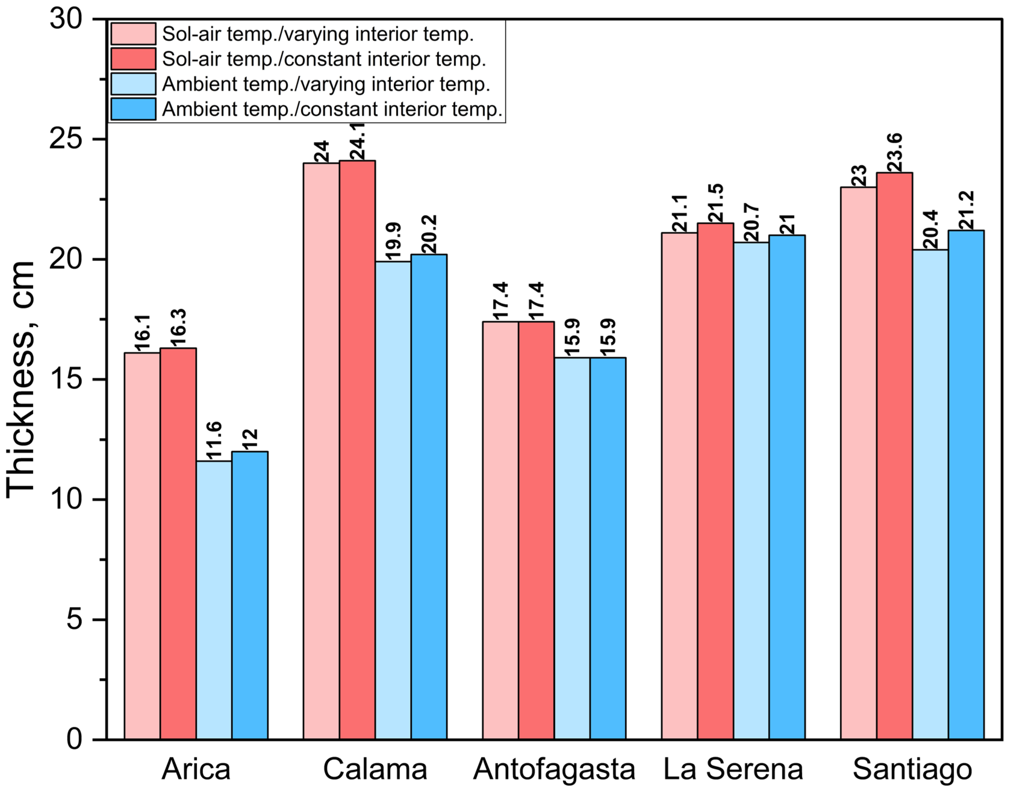
Figure 9 provides a graphical comparison of the optimum thicknesses of EPS thermal insulation in walls for the five study cities and all the methods used. In general, the greatest thicknesses are recorded in Calama and Santiago, where values can reach up to 24 cm, considering both variable and constant temperatures, as well as the effect of solar radiation.

The high thicknesses in Calama and Santiago are related to more extreme climatic conditions in summer and winter compared to the other cities. Therefore, the thermal insulation must address both heating and cooling issues.

According to the ECS, to comply with the maximum allowable thermal transmittance (U-value) in different climatic zones of the country, the wall configuration studied requires only 0.01 cm of insulation in the cities of Arica and Antofagasta. Therefore, even without additional insulation, the proposed solution already meets national requirements in those locations. In contrast, in Santiago and La Serena, the minimum insulation thickness required to meet standards is 2.6 cm, while in Calama it is 9.7 cm of EPS. Consequently, the insulation thicknesses obtained through the Life Cycle Cost Analysis (LCCA) methodology significantly exceed the values established by current national energy efficiency regulation.

The results suggest that considering solar radiation and using variable threshold temperatures better reflect thermal comfort needs. Additionally, the importance of selecting an appropriate technique for calculating degree days for the LCCA methodology to estimate the optimum thickness of thermal insulation has been discussed in previous works [21,30]. Another aspect is that for cities with a solar climate similar to Arica and Calama, it is important to consider global solar radiation to estimate the optimum wall thickness, as demonstrated in recent studies from different parts of the world [23,25,54]. However, the main problem lies in the availability of information on global solar radiation from different orientations and inclinations of building envelope elements. Although it is possible to use real measurement data of global solar radiation, this approach is quite complex and requires extensive instrumentation. Another alternative is the calculation of solar radiation for clear skies, as in the study by [4], but without considering geophysical aspects that affect the variation in global solar radiation, such as the presence of clouds, variation in atmospheric aerosols, etc. Therefore, the example presented in this work, using global solar radiation data from the Solar Explorer [34], represents a good alternative for considering the effects of solar radiation in various tasks and calculations related to building climatology in Chile.

Additionally, it is logical to deduce that for roofs, considering the effect of solar radiation will be mandatory in climate zones that are not as severe as those presented in this study. However, this will require additional studies and will depend on the initial construction solution of the roof in the search for the optimum insulation thickness. The consideration of constant temperatures increases the optimum thicknesses in all cases, as a constant annual temperature does not reflect the monthly variations in adaptive thermal comfort temperatures in each city with its corresponding climate, as illustrated in Figure 5 and Figure 6. Therefore, the application of constant temperatures can lead to a slight increase in the optimum thickness and unnecessary use of material. Although this difference is not significant, it can raise the carbon footprint of materials used in a construction project. Hence, the use of variable adaptive thermal comfort temperatures is appropriate for calculating HDDs and CDDs in the analyzed climates (hot arid, Mediterranean types) and should be included in the estimations of optimum wall and roof thicknesses using the LCCA methodology. Differences in insulation thicknesses can be quite notable (Figure 9), but to analyze the real effect on the energy demand of a project, the following section will be presented.

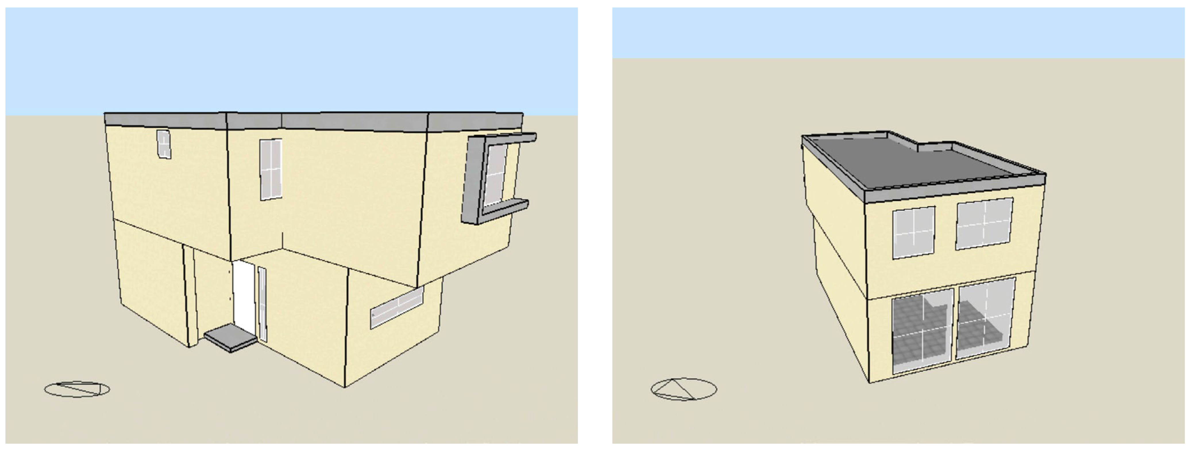
3.3. Validation Results of Optimum Insulation Thicknesses Through Energy Simulation

In the previous section, optimum insulation thickness values were established considering the effect of solar radiation and without this effect. This section presents the results of the annual energy demand simulation for heating and cooling of the studied house located in five cities for five optimum EPS thicknesses considering the effect of solar radiation, without this consideration, and for a wall with a constant insulation thickness of 3 cm (control case). The energy demand simulation was performed only for optimum thicknesses with constant threshold temperatures (see Figure 9). All energy demand results for heating and cooling of the studied house can be seen in

Table 13. Annual energy demand for cooling and heating of the studied house in the analyzed cities.

	With Solar Radiation Effect				Without Solar Radiation Effect				Control Case
	e, [cm]	U, [W/m2K]	Cooling, [kWh/m2]	Heating, [kWh/m2]	e, [cm]	U, [W/m2K]	Cooling, [kWh/m2]	Heating, [kWh/m2]	e, [cm]	U, [W/m2K]	Cooling, [kWh/m2]	Heating [kWh/m2]
Arica	16.3	0.19	12.1	2.2	12	0.25	11.9	2.5	3	0.74	10.6	4.7
Calama	24.1	0.13	3.7	22.7	20.2	0.16	3.2	25.9	3	0.74	1.2	49.4
Antofagasta	17.4	0.18	4.7	9.3	15.9	0.19	4.6	9.6	3	0.74	2.9	17.0
La Serena	21.5	0.15	2.3	23.2	21	0.15	2.1	25.6	3	0.74	1.2	41.9
Santiago	23.6	0.14	12.5	37.3	21.2	0.15	12.4	38.1	3	0.74	11.0	60.6

. For all cities, for the studied wall, considering the effect of solar radiation and without considering it in the LCCA methodology, there is not much difference in the results.

It can be highlighted that the results obtained from the energy simulation are within the range of permissible values for residential houses according to Chilean building standard ECS [38]. Thus, for the cities of Arica and Antofagasta, the energy demand values of a residential home for cooling and heating should not exceed 10 kWh/m² and 15 kWh/m², respectively. For the city of Calama and for climatic zone H, cooling demand must be around 0 kWh/m² and for heating not exceed 120 kWh/m². In La Serena and Santiago, the permissible value of the cooling demand must be less than 10 kWh/m² and for heating no greater than 77 kWh/m² and 71 kWh/m², respectively.

The greatest difference is observed in the city of Calama, where increasing the EPS thickness for walls from 20.2 cm to 24.1 cm would help reduce the annual heating demand from 25.9 kWh/m² to 22.7 kWh/m²; however, this would increase the cooling demand by 0.5 kWh/m². This is likely related to the high thermal mass of the studied wall type. On the other hand, in Arica, an increase of 12 cm of insulation in walls up to 16.3 cm also results in a slight increase in cooling demand, which is also related to the high thermal mass of the studied wall and applied to the analyzed house.

Similar results regarding the increase in cooling energy demand with the increase in wall thermal mass were observed in a study conducted in Saudi Arabia under arid climate conditions comparable to those of the present study [55]. Likewise, other researchers in Saudi Arabia working under extreme desert climates emphasize the importance of achieving a balance between thermal insulation and thermal mass to ensure cooling-efficient building designs [56]. In another study focused on public buildings, the authors observed that increasing the thermal mass of envelope components had only a modest effect on mitigating indoor overheating during periods of high outdoor temperatures [57].

In all studied cities, the use of the optimum thickness estimated based on the LCCA methodology reduces the total demand for heating and cooling by an average of 6–48%, similar to what was observed in a study conducted in Turkey [4]. Additionally, for these cities, the use of the optimum thermal insulation thickness for the analyzed house significantly reduces (46–86%) the heating demand.

In the case of the cities of Arica and Antofagasta, increasing the insulation from 3 cm to the optimum values defined by the LCCA methodology does not generate benefits in the energy efficiency of the analyzed house project. Therefore, the application of additional thermal insulation in cities with these climatic conditions is not as necessary for the analyzed house and wall type.

Despite significant differences in the optimum thermal insulation thickness obtained with or without considering the effect of solar radiation for the studied wall and house type, the energy demand simulation did not show significant differences in the variation in the energy performance of the studied house. Moreover, for cities with warmer and milder climates, the use of the optimum insulation thickness for the studied mass wall did not provide any energy benefit but rather the opposite effect. This highlights the importance of more in-depth studies on the application of the LCCA methodology to define optimum insulation thicknesses in different climatic zones for mass walls and to assess the feasibility of integrating this variable to improve the LCCA methodology.

4. Conclusions

An analysis of the effect of global solar radiation on the optimum thickness of thermal insulation for exterior walls in northern Chile was conducted using the LCCA methodology. A specific type of mass wall was analyzed, and the main conclusions were as follows:

The consideration of the sol–air temperature in determining the optimum insulation thickness for the studied wall is especially relevant in Arica and Calama. In Arica, this effect increases the insulation thickness by 39%, and in Calama, by 21%, with variable monthly temperatures indoors. For other cities, the difference was not significant. Although only one type of wall was analyzed, the results are sufficient to demonstrate the importance of solar radiation in the LCCA methodology for defining the optimum wall thickness.

The use of constant threshold temperatures for heating and cooling tends to increase the optimum insulation thickness studied, although not significantly, as these are based on averages derived from an adaptive thermal comfort model for the analyzed cities. This simplification facilitates the calculation but may not accurately reflect actual needs due to seasonal variations. It is recommended to use variable threshold temperatures adjusted monthly according to the adaptive thermal comfort model to obtain more precise and specific results. However, constant threshold temperatures can be useful for preliminary studies.

On the other hand, it was demonstrated that for the studied house, the influence of solar radiation on the results of the search for the optimum insulation thickness does not have a significant effect on its energy efficiency, due to the type of mass wall studied in this research. However, the LCCA methodology provides good results for optimum thermal insulation in cities such as Calama, La Serena, and Santiago, where the energy demand for heating predominates over cooling. Considering solar radiation and using the sol–air temperature instead of the ambient air temperature to define the optimal thermal insulation thickness through the Life Cycle Cost Analysis (LCCA) methodology helps reduce the cooling and heating energy demand of the studied house by 36% to 41% in the city of La Serena, and by 42% to 47% in the city of Calama.

For the cities of Arica and Antofagasta, the use of the optimum thickness defined based on the LCCA methodology did not provide energy improvements in the studied house, raising questions about the applicability of this methodology for mass walls and requiring future studies. Additionally, future studies should focus on roofs with high heat capacity and the consideration of the effect of solar radiation, which could undoubtedly affect the results of the LCCA methodology for determining the optimum insulation thickness and the energy performance of house and building projects.

References

1. Calvin, K.; Dasgupta, D.; Krinner, G.; Mukherji, A.; Thorne, P.W.; Trisos, C.; Romero, J.; Aldunce, P.; Barrett, K.; Blanco, G.; et al. IPCC, 2023: Climate Change 2023: Synthesis Report. Contribution of Working Groups I, II and III to the Sixth Assessment Report of the Intergovernmental Panel on Climate Change, 1st ed.; Core Writing Team, Lee, H., Romero, J., Eds.; Intergovernmental Panel on Climate Change (IPCC): Geneva, Switzerland, 2023. [Google Scholar]
2. Labaran, Y.H.; Mathur, V.S.; Muhammad, S.U.; Musa, A.A. Carbon Footprint Management: A Review of Construction Industry. Clean. Eng. Technol. 2022, 9, 100531. [Google Scholar] [CrossRef]
3. Díaz López, C.; Carpio, M.; Martín-Morales, M.; Zamorano, M. A Comparative Analysis of Sustainable Building Assessment Methods. Sustain. Cities Soc. 2019, 49, 101611. [Google Scholar] [CrossRef]
4. Köse Özturan, M.; Kurnuç Seyhan, A. Determination of Optimum Insulation Thickness of Building Walls According to Four Main Directions by Accounting for Solar Radiation: A Case Study of Erzincan, Türkiye. Energy Build. 2024, 304, 113871. [Google Scholar] [CrossRef]
5. Chen, Y.; Ren, Z.; Peng, Z.; Yang, J.; Chen, Z.; Deng, Z. Impacts of Climate Change and Building Energy Efficiency Improvement on City-Scale Building Energy Consumption. J. Build. Eng. 2023, 78, 107646. [Google Scholar] [CrossRef]
6. Berardi, U. A Cross-Country Comparison of the Building Energy Consumptions and Their Trends. Resour. Conserv. Recycl. 2017, 123, 230–241. [Google Scholar] [CrossRef]
7. Ai, W.; Wang, L.; Lin, X.; Zhang, S.; Bai, Y.; Chen, H. Mathematical and Thermo-Economic Analysis of Thermal Insulation for Thermal Energy Storage Applications. Renew. Energy 2023, 213, 233–245. [Google Scholar] [CrossRef]
8. Çomaklı, K.; Yüksel, B. Environmental Impact of Thermal Insulation Thickness in Buildings. Appl. Therm. Eng. 2004, 24, 933–940. [Google Scholar] [CrossRef]
9. Himmetoğlu, S.; Delice, Y.; Aydoğan, E.K.; Uzal, B. Energy Simulation Optimization for Building Insulation Materials. In Handbook of Smart Energy Systems; Springer International Publishing: Cham, Switzerland, 2023; pp. 653–665. ISBN 978-3-030-97939-3. [Google Scholar]
10. Pan, Y.; Zhu, M.; Lv, Y.; Yang, Y.; Liang, Y.; Yin, R.; Yang, Y.; Jia, X.; Wang, X.; Zeng, F.; et al. Building Energy Simulation and Its Application for Building Performance Optimization: A Review of Methods, Tools, and Case Studies. Adv. Appl. Energy 2023, 10, 100135. [Google Scholar] [CrossRef]
11. Zheng, Z.; Zhou, J.; Yang, Y.; Xu, F.; Liu, H. Economic Optimization of Exterior Wall Insulation in Chinese Office Buildings by Coupling Artificial Neural Network and Genetic Algorithm. Therm. Sci. Eng. Prog. 2024, 50, 102582. [Google Scholar] [CrossRef]
12. Kumar, D.; Alam, M.; Memon, R.A.; Bhayo, B.A. A Critical Review for Formulation and Conceptualization of an Ideal Building Envelope and Novel Sustainability Framework for Building Applications. Clean. Eng. Technol. 2022, 11, 100555. [Google Scholar] [CrossRef]
13. Amani, N. Developing a New Model to Optimize Thermal Insulation Thickness for Building Energy Efficiency. J. Renew. Energy Environ. 2024, 11, 118–131. [Google Scholar] [CrossRef]
14. Zhou, B.; Zhao, J.; Li, Y.; Gao, J.; Huang, B.; Wu, R.; Zhang, W.; Tan, B. Optimization Strategies of the Envelope Insulation for a Detached House Based on Load Sensitivity and Thermal Storage Performance. J. Build. Phys. 2024, 47, 496–525. [Google Scholar] [CrossRef]
15. Makawi, M.A.; Ahmed, W.; Kenawy, H.S.; Abd El Fattah, A. A Novel Validated Method to Determine the Relationship Between Insulation Thickness and the Annual Cooling Cost in Desert Climates. Appl. Sci. 2025, 15, 2839. [Google Scholar] [CrossRef]
16. Daouas, N.; Hassen, Z.; Aissia, H.B. Analytical Periodic Solution for the Study of Thermal Performance and Optimum Insulation Thickness of Building Walls in Tunisia. Appl. Therm. Eng. 2010, 30, 319–326. [Google Scholar] [CrossRef]
17. Di Filippo, R.; Maracchini, G.; Albatici, R.; Di Maggio, R.; Bursi, O.S. A Novel Prescriptive Approach for Buildings’ Insulation Design Considering Embodied Carbon. Renew. Sustain. Energy Rev. 2025, 212, 115369. [Google Scholar] [CrossRef]
18. Annibaldi, V.; Cucchiella, F.; De Berardinis, P.; Rotilio, M.; Stornelli, V. Environmental and Economic Benefits of Optimal Insulation Thickness: A Life-Cycle Cost Analysis. Renew. Sustain. Energy Rev. 2019, 116, 109441. [Google Scholar] [CrossRef]
19. Sisman, N.; Kahya, E.; Aras, N.; Aras, H. Determination of Optimum Insulation Thicknesses of the External Walls and Roof (Ceiling) for Turkey’s Different Degree-Day Regions. Energy Policy 2007, 35, 5151–5155. [Google Scholar] [CrossRef]
20. López-Ochoa, L.M.; Las-Heras-Casas, J.; López-González, L.M.; García-Lozano, C. Energy Renovation of Residential Buildings in Cold Mediterranean Zones Using Optimized Thermal Envelope Insulation Thicknesses: The Case of Spain. Sustainability 2020, 12, 2287. [Google Scholar] [CrossRef]
21. Verichev, K.; Serrano-Jiménez, A.; Carpio, M.; Barrios-Padura, Á.; Díaz-López, C. Influence of Degree Days Calculation Methods on the Optimum Thermal Insulation Thickness in Life-Cycle Cost Analysis for Building Envelopes in Mediterranean and Semi-Arid Climates. J. Build. Eng. 2023, 79, 107783. [Google Scholar] [CrossRef]
22. Márquez, A.C.; Parra Márquez, C.; Gómez Fernández, J.F.; López Campos, M.; González-Prida Díaz, V. Life Cycle Cost Analysis. In Asset Management; Springer: Dordrecht, The Netherlands, 2012; pp. 81–99. ISBN 978-94-007-2723-6. [Google Scholar]
23. Aktemur, C.; Çakır, M.T.; Çakır, M.F. Optimising of Thermal Insulation Thickness Based on Wall Orientations and Solar Radiation Using Heating-Degree Hour Method. Case Stud. Therm. Eng. 2024, 60, 104725. [Google Scholar] [CrossRef]
24. Nematchoua, M.K.; Raminosoa, C.R.R.; Mamiharijaona, R.; René, T.; Orosa, J.A.; Elvis, W.; Meukam, P. Study of the Economical and Optimum Thermal Insulation Thickness for Buildings in a Wet and Hot Tropical Climate: Case of Cameroon. Renew. Sustain. Energy Rev. 2015, 50, 1192–1202. [Google Scholar] [CrossRef]
25. Li, T.; Liu, Q.; Mao, Q.; Chen, M.; Ma, C.; Wang, D.; Liu, Y. Optimization Design Research of Insulation Thickness of Exterior Wall Based on the Orientation Difference of Solar Radiation Intensity. Appl. Therm. Eng. 2023, 223, 119977. [Google Scholar] [CrossRef]
26. Li, H.; Zhong, K.; Yu, J.; Kang, Y.; Zhai, Z. Solar Energy Absorption Effect of Buildings in Hot Summer and Cold Winter Climate Zone, China. Sol. Energy 2020, 198, 519–528. [Google Scholar] [CrossRef]
27. Hashim, H.M.; Sokolova, E.; Derevianko, O.; Solovev, D.B. Cooling Load Calculations. IOP Conf. Ser. Mater. Sci. Eng. 2018, 463, 032030. [Google Scholar] [CrossRef]
28. Zurita, A.; Castillejo-Cuberos, A.; García, M.; Mata-Torres, C.; Simsek, Y.; García, R.; Antonanzas-Torres, F.; Escobar, R.A. State of the Art and Future Prospects for Solar PV Development in Chile. Renew. Sustain. Energy Rev. 2018, 92, 701–727. [Google Scholar] [CrossRef]
29. Verichev, K.; Carpio, M. Climatic Zoning for Building Construction in a Temperate Climate of Chile. Sustain. Cities Soc. 2018, 40, 352–364. [Google Scholar] [CrossRef]
30. Carpio, M.; López-Ochoa, L.M.; Las-Heras-Casas, J.; Verichev, K. Influence of Heating Degree Day Calculation Methods in Designing the Thermal Envelope of Buildings. J. Build. Eng. 2022, 46, 103604. [Google Scholar] [CrossRef]
31. Verichev, K.; Zamorano, M.; Salazar-Concha, C.; Carpio, M. Analysis of Climate-Oriented Researches in Building. Appl. Sci. 2021, 11, 3251. [Google Scholar] [CrossRef]
32. Sarricolea, P.; Herrera-Ossandon, M.; Meseguer-Ruiz, Ó. Climatic Regionalisation of Continental Chile. J. Maps 2017, 13, 66–73. [Google Scholar] [CrossRef]
33. Ministry of Energy—Chile Explorador Solar. Available online: https://solar.minenergia.cl/exploracion (accessed on 14 July 2025).
34. Molina, A.; Falvey, M.; Rondanelli, R. A Solar Radiation Database for Chile. Sci. Rep. 2017, 7, 1–11. [Google Scholar] [CrossRef]
35. López-Ochoa, L.M.; Las-Heras-Casas, J.; López-González, L.M.; Olasolo-Alonso, P. Environmental and Energy Impact of the EPBD in Residential Buildings in Hot and Temperate Mediterranean Zones: The Case of Spain. Energy 2018, 161, 618–634. [Google Scholar] [CrossRef]
36. Las-Heras-Casas, J.; López-Ochoa, L.M.; Paredes-Sánchez, J.P.; López-González, L.M. Implementation of Biomass Boilers for Heating and Domestic Hot Water in Multi-Family Buildings in Spain: Energy, Environmental, and Economic Assessment. J. Clean. Prod. 2018, 176, 590–603. [Google Scholar] [CrossRef]
37. Mourshed, M. Relationship between Annual Mean Temperature and Degree-Days. Energy Build. 2012, 54, 418–425. [Google Scholar] [CrossRef]
38. Ministerio de Vivienda y Urbanismo. Estándares de Construcción Sustentable Para Viviendas de Chile; Segunda edición, versión oficial, febrero de 2018; Ministerio de Vivienda y Urbanismo: Santiago, Chile, 2018; ISBN 978-956-9432-52-1.
39. ASHRAE. 2017 ASHRAE Handbook: Fundamentals, SI ed.; American Society of Heating, Refrigerating and Air-Conditioning Engineers, Ed.; ASHRAE: Atlanta, Georga, 2017; ISBN 978-1-939200-58-7. [Google Scholar]
40. Brager, G.S.; De Dear, R.J. Thermal Adaptation in the Built Environment: A Literature Review. Energy Build. 1998, 27, 83–96. [Google Scholar] [CrossRef]
41. Chilean Government. Norma Chilena Nch 853:2021, Acondicionamiento Termico. 2021. Available online: https://ecommerce.inn.cl/nch853202179509 (accessed on 17 June 2025).
42. Xiao, G.; He, N.; Yin, K.; Zhang, X.; Xie, J. Comparative Study of Sol-Air Temperature Models in the Tropical Island Based on Measured Data. E3S Web Conf. 2023, 396, 05009. [Google Scholar] [CrossRef]
43. Karn, A.; Chintala, V.; Kumar, S. An Investigation into Sky Temperature Estimation, Its Variation, and Significance in Heat Transfer Calculations of Solar Cookers. Heat Trans. Asian Res. 2019, 48, 1830–1856. [Google Scholar] [CrossRef]
44. Evangelisti, L.; Guattari, C.; Asdrubali, F. On the Sky Temperature Models and Their Influence on Buildings Energy Performance: A Critical Review. Energy Build. 2019, 183, 607–625. [Google Scholar] [CrossRef]
45. Las-Heras-Casas, J.; López-Ochoa, L.M.; López-González, L.M.; Olasolo-Alonso, P. Energy Renovation of Residential Buildings in Hot and Temperate Mediterranean Zones Using Optimized Thermal Envelope Insulation Thicknesses: The Case of Spain. Appl. Sci. 2021, 11, 370. [Google Scholar] [CrossRef]
46. Kurekci, N.A. Determination of Optimum Insulation Thickness for Building Walls by Using Heating and Cooling Degree-Day Values of All Turkey’s Provincial Centers. Energy Build. 2016, 118, 197–213. [Google Scholar] [CrossRef]
47. Omle, I.; Kovács, E.; Bolló, B. Applying Recent Efficient Numerical Methods for Long-Term Simulations of Heat Transfer in Walls to Optimize Thermal Insulation. Results Eng. 2023, 20, 101476. [Google Scholar] [CrossRef]
48. Central Bank of Chile Base de Datos Estadísticos (BDE). Available online: https://si3.bcentral.cl/siete (accessed on 14 July 2025).
49. Chile Falabella 1×0.5m 50 mm Paquete 12 Planchas|Sodimac. Available online: https://www.falabella.com/falabella-cl/product/110318582/1x0,5m-50-mm-paquete-12-planchas/110318586 (accessed on 14 July 2025).
50. CGE CGE Chile. Available online: https://www.cge.cl/ (accessed on 14 July 2025).
51. Enel Enel Chile—enel.cl. Available online: https://enel.cl/content/enel-cl/es.html (accessed on 14 July 2025).
52. 90.1 User’s Manual: ANSI/ASHRAE/IES Standard 90.1-2010: Energy Standard for Buildings Except Low-Rise Residential Buildings; American Society of Heating, Refrigerating and Air-Conditioning Engineers, Ed.; American Society of Heating, Refrigerating and Air-Conditioning Engineers: Atlanta, GA, USA, 2011; ISBN 978-1-933742-96-0. [Google Scholar]
53. Stasinopoulos, T.N. Comparing Insolation on Building Façades in Five Different Climates. ECAM 2023, 30, 1835–1863. [Google Scholar] [CrossRef]
54. Fohagui, F.C.V.; Koholé, Y.W.; Alombah, N.H.; Asoh, D.A.; Tchuen, G. Optimum Insulation Thickness and Exergy Savings of Building Walls in Bamenda: A Comparative Analysis. Energy Storage Sav. 2024, 3, 60–70. [Google Scholar] [CrossRef]
55. Alayed, E.; Bensaid, D.; O’Hegarty, R.; Kinnane, O. Thermal Mass Impact on Energy Consumption for Buildings in Hot Climates: A Novel Finite Element Modelling Study Comparing Building Constructions for Arid Climates in Saudi Arabia. Energy Build. 2022, 271, 112324. [Google Scholar] [CrossRef]
56. Alqahtani, M.; Alshahrani, M.; Alaidroos, A.; Fageha, M.K. Optimal Thermal Diffusivity of Residential Building Envelopes to Improve Cooling Energy Efficiency for Saudi Arabia’s Climate Zones. J. Archit. Eng. 2024, 30, 04024015. [Google Scholar] [CrossRef]
57. Cheng, R.; Zhang, N.; Zhang, W.; Sun, Y.; Yin, B.; Gao, W. Impact of Thermal Mass, Window Performance, and Window–Wall Ratio on Indoor Thermal Dynamics in Public Buildings. Buildings 2025, 15, 1757. [Google Scholar] [CrossRef]
Figure 1. Location of studied cities.
Buildings 15 02580 g001
Figure 2. Accumulated global solar radiation during the year 2016 in the studied cities for three wall orientations (W-west, N-north, and E-east).
Buildings 15 02580 g002
Figure 3. Box-plots of hourly ambient temperature values in the study cities for the year 2016.
Buildings 15 02580 g003
Figure 4. Construction solution for the studied wall (numbers correspond to the layer numbers in Table 2).
Buildings 15 02580 g004
Figure 5. Monthly threshold temperatures for heating by study cities according to ECS.
Buildings 15 02580 g005
Figure 6. Monthly threshold temperatures for cooling by study cities according to ECS.
Buildings 15 02580 g006
Figure 7. Typical house in northern Chile used for energy simulation.
Buildings 15 02580 g007
Figure 8. Main meteorological parameters from the epw files used for the energy simulation: (a)–Temperature; (b)–Normal solar Radiation; (c)–Diffuse horizontal solar radiation.
Buildings 15 02580 g008
Figure 9. Comparison of optimum thicknesses—average value for 3 orientations (sol–air temp) and ambient temperature for south orientation (ambient temp).
Buildings 15 02580 g009