Prediction Model of Household Carbon Emission in Old Residential Areas in Drought and Cold Regions Based on Gene Expression Programming

Abstract

To support the national goals of carbon peaking and carbon neutrality, this study proposes a household carbon emission prediction model based on Gene Expression Programming (GEP) for low-carbon retrofitting of aging residential areas in arid-cold regions. Focusing on 15 typical aging communities in Kundulun District, Baotou City, a 17-dimensional dataset encompassing building characteristics, demographic structure, and energy consumption patterns was collected through field surveys. Key influencing factors (e.g., electricity usage and heating energy consumption) were selected using Pearson correlation analysis and the Random Forest (RF) algorithm. Subsequently, a hybrid prediction model was constructed, with its parameters optimized by minimizing the root mean square error (RMSE) as the fitness function. Experimental results demonstrated that the model achieved an R² value of 0.81, reducing RMSE by 77.1% compared to conventional GEP models and by 60.4% compared to BP neural networks, while significantly improving stability. By combining data dimensionality reduction with adaptive evolutionary algorithms, this model overcomes the limitations of traditional methods in capturing complex nonlinear relationships. It provides a reliable tool for precision-based low-carbon retrofits in aging residential areas of arid-cold regions and offers a methodological advance for research on building carbon emission prediction driven by urban renewal.

1. Introduction

Under the accelerating global climate governance framework, the building sector contributes 23% of total societal carbon emissions IPCC, 2022, making its low-carbon transition a critical pathway toward achieving carbon peaking and neutrality targets. China’s Energy Conservation and Carbon Reduction Action Plan (2024–2025) explicitly emphasizes breaking through energy efficiency barriers in existing buildings in northern cold regions [1]. As one of the first national low-carbon pilot cities, Baotou has accumulated extensive practical experience in carbon reduction initiatives. The city has established a 1 + 20 + 91 policy system for carbon peaking and neutrality, integrating energy-saving efforts across industrial, building, and transportation sectors. It has been designated a national pilot city for clean heating in northern regions, securing a three-year central government grant of 900 million yuan to support renewable energy retrofits and energy efficiency upgrades in aging residential areas, providing a significant reference for low-carbon urban transformation in arid-cold regions.

Existing studies highlight Baotou’s unique challenges as a heavy-industry city, where coal accounts for over 60% of the energy mix, and carbon intensity in steel and rare earth industries exceeds the national average [2]. These characteristics have driven the city to explore innovative low-carbon pathways [3]. Academic research on Baotou’s low-carbon development has primarily focused on industrial restructuring and clean energy substitution. However, current studies predominantly focus on new buildings or temperate climates, with limited attention to aging residential areas in arid-cold regions. These communities often face aging building envelopes, high heating energy consumption, and rigid energy-use patterns due to an aging population, posing significant challenges for carbon emission prediction due to complex data dimensions and pronounced nonlinear characteristics [4].

Traditional prediction models, such as BP neural networks, often fall into local optima when handling high-dimensional heterogeneous data, while classical Gene Expression Programming (GEP) lacks effective feature selection mechanisms to balance model complexity and generalization ability. To address these limitations, this study proposes a hybrid CA–RF–GEP modeling framework:

Spatial Noise Reduction: Cellular Automata (CA) theory is applied to extract local spatial correlations and reduce data noise.

Feature Selection: The Random Forest (RF) algorithm quantifies multi-factor contribution degrees, identifying seven core driving factors (e.g., electricity consumption X₁₆, heating energy use X₁₇).

Model Construction: A CA–RF–GEP predictive model is developed for small-sample scenarios.

Using 625 samples of 17-dimensional data (building physical attributes, household demographics, and sub-item energy consumption) from 15 aging residential areas in Kundulun District, Baotou, this study breaks the limitation of relying solely on macro-level statistical yearbook data in existing research. Comparative experiments with conventional GEP and BP neural networks validate the CA–RF–GEP model’s significant advantages in prediction accuracy and stability. This research not only fills the methodological gap in carbon emission prediction for aging residential areas in arid-cold regions but also supports Baotou’s *14th Five-Year Plan* targets (a 26.8% reduction in industrial energy intensity and a 47.46% reduction in water use). The proposed framework offers methodological innovation for assessing carbon reduction potential in high-latitude arid-cold aging communities and provides scientific evidence for urban renewal policies under the dual carbon goals.

2. Materials and Methods

This section aims to clarify the data sources, programming environments, and computational programs used in the study before introducing the detailed application program. This study integrates theoretical formulas with computational simulation and machine learning techniques for structural optimization. The method is divided into the following key stages.

2.1. Theoretical Framework and Structural Modeling (Hybrid Algorithm Based on GEP)

The CA–RF–GEP predictive model was developed within the PyCharm Community Edition 2023 (Python 3.8) environment [5] through a three-phase computational framework. Cellular Automata (CA) theory was employed to analyze local spatial correlations, effectively mitigating data noise through its inherent neighborhood interaction mechanism. The Random Forest (RF) algorithm was implemented to quantitatively assess multi-factor contributions, enabling the scientific identification and screening of core driving factors via feature importance ranking. We integrated these optimized components to establish a robust Gene Expression Programming (GEP)-based prediction model specifically designed for small-sample scenarios.

2.2. Simulation Environment

All analyses and calculations were conducted using PyCharm Community Edition 2023 (Python 3.8). Python boasts extensive ecological support in the field of scientific computing, including libraries such as NumPy 1.24, SciPy 1.10, and Matplotlib 3.7. When utilizing commonly used matrix computation libraries like NumPy 1.24 and SciPy 1.10, this version of PyCharm intelligently offers code completion and parameter hints.

2.3. Machine Learning: Gene Expression Programming (GEP)

Model training was conducted in Python using the NumPy and Pandas libraries. The training and test datasets were randomly split from the original dataset, with 80% allocated for training and 20% for testing to ensure robust model evaluation.

2.4. Optimization Algorithm: Adjustment Based on Population Diversity

Algorithm performance was evaluated in Python through multiple experiments, analyzing convergence behavior under different iteration counts. By adjusting the optimization algorithm, convergence was achieved with a population size of 100 and 2000 iterations, demonstrating the effectiveness of population diversity adjustment in balancing exploration and exploitation.

2.5. Validation and Comparison

The CA–RF–GEP algorithm model was compared with the conventional GEP algorithm model and the BP neural network algorithm model under identical datasets and computational environments. Model performance was evaluated using five metrics: the coefficient of determination (R²), root mean square error (RMSE), mean absolute error (MAE), relative root squared error (RRSE), and mean absolute percentage error (MAPE).

3. Methodology

3.1. Structural Analyses (GEP)

Genetic Expression Programming (GEP) is a bio-inspired algorithm that automatically discovers mathematical expressions in data by simulating natural selection and genetic mechanisms. Its primary advantages include high efficiency and stability, effectively addressing the tree structure imbalance issues inherent in traditional genetic programming [6]. GEP employs a linear encoding strategy where genes are divided into head and tail segments: the head contains both function symbols and terminals, while the tail consists solely of terminals. This structural design enhances algorithmic efficiency and reliability.

The fundamental unit of a GEP chromosome is the gene, which also comprises two components: the head and tail [7]. The head length h is predefined based on problem complexity, while the tail length t is calculated as

$$t=h\times \left(n-1\right)+1$$

where n denotes the maximum arity.

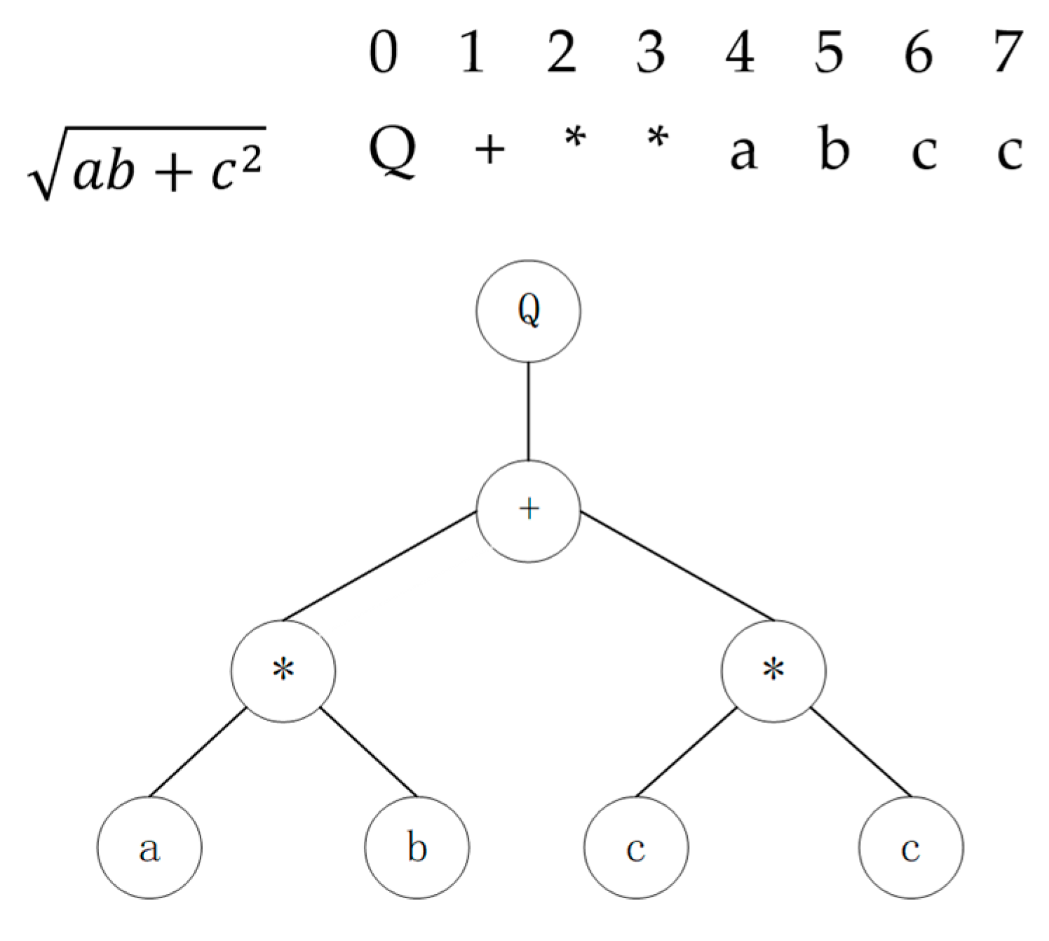
In the GEP algorithm, gene language and expression tree language correspond to the genotype and phenotype, respectively. These representations undergo bidirectional mapping: as shown in Figure 1, chromosomal encoding operates at the genotype level, while mathematical expressions are generated through hierarchical traversal of the expression tree, enabling transformation from abstract genetic structures to concrete phenotypes.

In GEP, there are usually three methods for calculating the fitness function:

Absolute Error-Based Fitness:

$$f_i=\sum _{j=1}^n\left(M-\left|C_{\left(i,j\right)}-T_j\right|\right)$$

Relative Error-Based Fitness:

$$f_i=\sum _{j=1}^n(M-|{\displaystyle \frac{C_{\left(i,j\right)}-T_j}{T_j}}\times 100\left|\right)$$

Logical Synthesis Problem Fitness:

$$\mathrm{If} n\ge 1/2C_t,\mathrm{then} f_i=n; \mathrm{else} f_i=1$$

The aforementioned fitness functions exhibit limitations in practical applications, including sensitivity to outliers and insufficient balance between model complexity and generalization. To address these challenges, this study adopts the root mean square error RMSE as the fitness function, as follows:

$$RMSE=\sqrt{{\displaystyle \frac{1}{n}}\sum _{i=1}^n{\left(y_i-{\widehat{y}}_i\right)}^2}$$

3.2. Selected of Discuss and Verification

3.2.1. Experimental Data Source

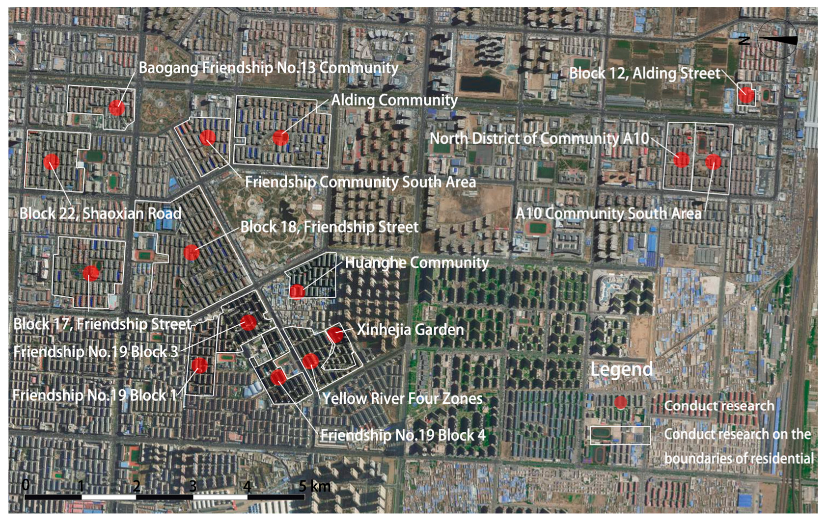
The data collection was conducted in the elderly residential area of Kundulun District, Baotou City in 2024. Fifteen representative residential areas constructed before 2000 were selected as samples (see Figure 2), ensuring the dataset’s typicality and representativeness. These areas were chosen based on spatial distribution and building typology to reflect the common characteristics of aging communities in arid-cold regions.

A total of 750 questionnaires were distributed. Following manual screening, 625 valid responses were confirmed. Detailed statistical parameters are presented in

Table 1. Summary table of research data compilation.

	X1/m2	X2/Person	X3/Housedhold	X4/Headcount	X5/Headcount	X6/Headcount	X7/Headcount	X8/Headcount	X9
Min	33	5	60	1	0	0	0	0	1
Max	165	120	6876	6	1	2	5	3	3
Mean	67.73	37.54	2444.39	2.31	0.05	0.13	0.53	1.61	2.53
Md	68	32	2322	2	0	0	0	2	3
SD	14.24	26.35	1537.42	0.97	0.21	0.37	0.88	0.72	0.67
	X10/many	X11	X12	X13	X14/RMB	X15/RMB	X16/RMB	X17/RMB	y/kgCO2e
Min	1	0	1	0	70	80	100	350	239.06
Max	7	0.30	2	24,000	1450	1300	3000	3700	9913.92
Mean	4.26	0.13	1.10	255.52	489.72	430.77	834.30	1461.54	1062.86
Md	4	0.10	1	0	450	400	800	1400	939.11
SD	1.98	0.09	0.29	1622.03	191.11	194.64	407.58	322.17	715.93

.

The detailed variable indicators in Table 1 are explained in

Table 2. Explanation of research variables and indicators.

Variable	Description	Variable	Description
X1	Building Area	X10	Number of Entrances
X2	Number of Buildings	X11	Green Space Ratio (%)
X3	Number of Households	X12	Road Structure Type
X4	Total Population	X13	Gasoline Consumption
X5	Population aged 0–4 years	X14	Natural Gas Consumption
X6	Population aged 5–14 years	X15	Water Consumption
X7	Population aged 15–49 years	X16	Electricity Consumption
X8	Population aged 50+ years	X17	Heating Energy Consumption
X9	Construction Year	Y	Total Carbon Emissions (kg CO2e)

.

3.2.2. Determination of Carbon Emission Factors

Carbon emission factors serve as metrics quantifying CO₂ emissions from specific activities or production processes. Their determination relies on specialized experimental research; however, numerical values vary across studies due to differences in experimental objectives and methodologies. The Standard for Building Carbon Emission Calculation (GB/T 51366-2019) provides baseline emission factors, but these cannot fully meet actual accounting needs and require supplementation based on practical conditions.

The carbon emission factors used in this study are primarily referenced from the following authoritative sources:

National Standards: Standard for Building Carbon Emission Calculation (GB/T 51366-2019), providing baseline emission coefficients for building-related activities.

Peer-Reviewed Literature: Academic publications certified by authoritative institutions, including cited references [8,9,10].

Authoritative Reports: Research reports and statistical yearbooks issued by governmental or international organizations.

Industry Guidelines: Regulatory documents and technical standards promulgated by relevant industry associations.

Methodology for Fossil Fuel Emission Factor Calculation

The fossil fuel CO₂ emission factors employed in this study were calculated according to the 2006 IPCC Guidelines for National Greenhouse Gas Inventories, incorporating energy calorific values from the General Rules for Comprehensive Energy Consumption Calculation (GB/T 2589-2008) [11] and fossil fuel CO₂ emission factors specified in the Standard for Building Carbon Emission Calculation (GB/T 51366-2019) [12]. Detailed calculation results are summarized in

Table 3. Common energy carbon emission factors.

Energy Name	Unit Calorific Value CO2 Emission Factor (tCO2e/TJ)	Average Low-Level Heat Generation (kJ/kg)	Carbon Emission Factor (kgCO2e/kg)
gasoline	67.91	43,070	2.925
diesel oil	72.59	42,652	3.096
kerosene	70.43	43,070	3.033

Note: Data are sourced from the Standard for Building Carbon Emission Calculation (GB/T 51366-2019) and the General Rules for Comprehensive Energy Consumption Calculation (GB/T 2589-2008).

.

The carbon emission factor for fossil fuels is calculated as follows:

$$Q_{ii}=C_{sc}\times q$$

Electricity Carbon Emissions

Due to regional variations in dominant power generation mixes, carbon emission factors exhibit spatial heterogeneity. This study adopts the 2019 regional grid baseline emission factors from the Baseline Emission Factors for Regional Power Grids in China issued by the Department of Climate Change, Ministry of Ecology and Environment [10]. The finalized dataset, reflecting regional disparities in power generation structures (e.g., coal-dominant versus renewable-energy-dominant systems), is summarized in

Table 4. Carbon emission factors of China’s regional power grid.

Grid Name	Carbon Emission Factor (kgCO2e/kwh)	Covering Provinces and Cities
North China Regional Power Grid	0.9419	Beijing, Tianjin, Hebei Province, Shanxi Province, Shandong Province, Inner Mongolia
Northeast Regional Power Grid	1.0826	Liaoning Province, Jilin Province, Heilongjiang Province
East China Regional Power Grid	0.7921	Shanghai, Jiangsu Province, Zhejiang Province, Anhui Province, Fujian Province
Central China Regional Power Grid	0.8587	Henan Province, Hubei Province, Hunan Province, Jiangxi Province, Sichuan Province, Chongqing City
Northwest Regional Power Grid	0.8922	Shaanxi Province, Gansu Province, Qinghai Province, Ningxia Province, Xinjiang Province
Southern Regional Power Grid	0.8042	Guangdong Province, Guangxi Autonomous Region, Yunnan Province, Guizhou Province, Hainan Province

.

3.2.3. Normalization of Experimental Data

The identified carbon emission influencing factors in aging residential retrofits exhibit significant variations due to diverse units and characteristics of the variables. To achieve dimensional homogeneity, all factor data were normalized using the following formula:

$$X_i^{\prime }={\displaystyle \frac{X_i-X_{imin}}{X_{imax}-X_{imin}}}$$

3.2.4. GEP Model Establishment

Characterized by prolonged duration, extensive scope, and complex operational components, aging residential retrofits inherently lead to complex carbon emission influencing factors. To address this, this study employs a machine learning-based approach to identify and analyze key influencing factors. A database of 625 samples was constructed, with the dataset partitioned into training and validation sets at a 4:1 ratio to ensure robust model calibration and performance evaluation.

Preliminary Screening of Carbon Emission Factors

To address high-dimensional data redundancy in carbon emission prediction for aging residential retrofits, this study employs Pearson correlation analysis for variable selection. The correlation coefficient r (where r ∈ [−1, 1]) quantifies linear relationships between variables:

• |r| = 1: Perfect correlation
• |r| = 0: No correlation

The absolute value of r directly indicates association strength between two factors—larger absolute values denote stronger correlations. Specifically, r represents the correlation between carbon emission influencing factors and total carbon emissions in aging residential retrofits. The calculation formula is:

$$r={\displaystyle \frac{\sum _{i=1}^n(X_i-\overline{X})(Y_i-\overline{Y})}{\sqrt{\sum _{i=1}^n{(X_i-\overline{X})}^2}\sqrt{\sum _{i=1}^n{(Y_i-\overline{Y})}^2}}}$$

The correlation analysis quantifies relationships between independent variables (carbon emission influencing factors) and the dependent variable (total carbon emissions) in aging residential retrofits. Variables with absolute correlation coefficients |r| > 0.4 were selected for inclusion in the preliminary carbon emission factor system. These factors, detailed in

Table 5. Correlation analysis results.

	X1	X2	X3	X4	X5	X6	X7
r	0.202	−0.142	0.081	−0.076	0.293	0.218	0.26
Sig	0	0	0.044	0.056	0	0	0
	X8	X9	X10	X11	X12	X13	X14
r	−0.066	−0.024	−0.106	−0.071	0.074	0.873	0.425
Sig	0.101	0.544	0.008	0.075	0.065	0	0
	X15	X16	X17
r	0.417	0.505	0.242
Sig	0	0	0

, form the basis for subsequent model development.

In predictive modeling, a two-tailed p-value (Sig) < 0.05 indicates statistically significant relationships between variables, even with relatively low correlation coefficients. This study adopts a dual-criteria selection approach: variables must satisfy both |r| > 0.4 and Sig < 0.05 to ensure robustness in the emission factor system for low-carbon retrofits of aging residential areas. The final set of indicators, rigorously validated through this screening process, forms the basis for subsequent analysis and is summarized in

Table 6. Partial correlation analysis results.

	X3	X4	X8	X9	X10	X11	X12
r	0.274	0.281	0.299	0.164	−0.026	−0.063	−0.029
Sig	0	0	0	0	0.515	0.117	0.464

.

Feature Importance Analysis via Random Forest

Dimensionality reduction techniques mitigate overfitting by compressing data features without increasing sample size [13]. Random Forest (RF), an ensemble learning model comprising multiple decision trees, employs bootstrap resampling to generate diverse training datasets through random sampling with replacement. Each decision tree is trained on these bootstrapped samples, collectively forming the Random Forest architecture.

The model calculates feature importance based on data fit, quantifying each variable’s contribution to prediction accuracy. The resultant importance coefficients for all indicators are presented in

Table 7. Calculation results of random forest model.

Variable	Importance Coefficient	Variable	Importance Coefficient
X1	0.07	X8	0.01
X2	0.04	X9	0.01
X3	0.04	X13	0.02
X4	0.02	X14	0.27
X5	0.01	X15	0.10
X6	0.01	X16	0.36
X7	0.03	X17	0.05

, highlighting the relative significance of factors within the aging residential carbon emission prediction framework.

Algorithm Construction Parameters

This study employed PyCharm Community Edition 2023 as the development environment to construct predictive models using genetic programming techniques. The model configuration involved key parameters including number of genes, chromosome count, and linkage functions, which were systematically optimized through iterative testing and parameter tuning. The finalized optimal parameter set, determined via cross-validation, is presented in

Table 8. GEP algorithm parameter settings.

Parameter Settings	Parameter Values	Parameter Settings	Parameter Values
number of iterations	2000	mutation rate	0.05
population size	100	IS transposition rate	0.1
Gene head length	12	RIS transposition rate	0.1
Number of chromosomes	5	Gene transposition rate	0.1
Copula	+	Single point recombination rate	0.3
Gene recombination rate	0.1	Two-point recombination rate	0.3

.

The terminal symbol set was defined as {a, b, c, d, e, f, g, h}, corresponding to the selected indicators {X₁, X₂, X₃, X₇, X₁₄, X₁₅, X₁₆, X₁₇}. A relative-error-based fitness function was adopted as the evaluation criterion, with the function symbol set comprising {+, −, ×, ÷, sin, cos, tan, sqrt, ln, max(arity)}.

3.3. Differences Between the Codes and Original Method

The CA–RF–GEP algorithm fundamentally differs from traditional GEP in modeling logic, data processing, and performance outcomes. The traditional GEP approach directly constructs mathematical models based on gene expression programming, optimizing expression structures through genetic operations like crossover and mutation. However, its lack of effective data preprocessing and feature selection mechanisms makes it prone to local optima and overfitting when handling high-dimensional heterogeneous data. 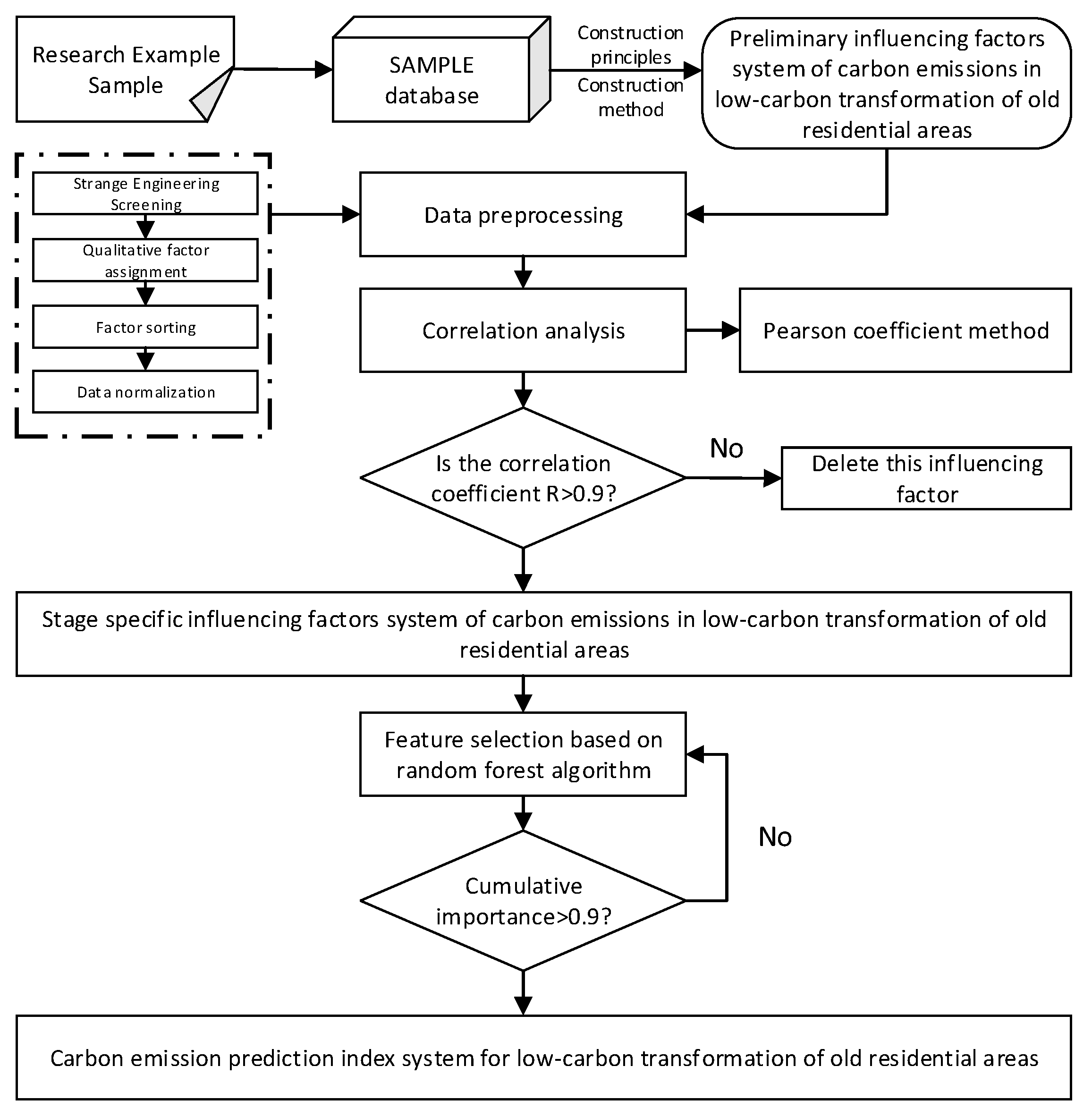In the Kundulun District aging residential case study (Baotou City), the traditional GEP model achieved a coefficient of determination (R²) of only 0.44 with a root mean square error (RMSE) of 682.00 kgCO₂e, demonstrating inadequate capability for capturing complex nonlinear relationships. In contrast, the CA–RF–GEP algorithm leverages a hybrid architecture (Figure 3) to achieve synergistic effects in noise reduction, feature selection, and model optimization:

1.

Data Denoising and Feature Selection

Cellular Automata (CA) Module: Using Pearson correlation analysis (∣r∣ > 0.4, Sig < 0.05), the CA module eliminates low-correlation variables (e.g., X₅, X₆), effectively reducing noise interference from building envelope aging and heterogeneous energy-use behaviors.

Random Forest (RF) Module: Leveraging feature importance coefficients, the RF module identifies seven key drivers—including electricity consumption (X₁₆, weight: 0.36) and heating energy use (X₁₇, weight: 0.05)—compressing input dimensionality from 17 to 7 features. This significantly mitigates the curse of dimensionality while preserving critical predictive information.

2.

Adaptive Modeling Optimization

Optimized GEP Module: The enhanced GEP component employs RMSE as the fitness function with parameter configurations including gene head length *h* = 12 and population size 100. Through iterative experimentation, the model achieves rapid convergence within 2000 generations, attaining final performance of R² = 0.81 and RMSE = 156.13 kgCO₂e. This represents an 83.6% improvement in R² and 77.1% reduction in RMSE compared to traditional GEP.

3.

Performance Advantages and Limitations

The CA–RF–GEP model maintains high stability even under extreme sample scenarios (maximum deviation: 9674.68 kgCO₂e) with a mean absolute percentage error (MAPE) of only 9.4%, while demonstrating significantly higher computational efficiency than conventional GEP models. However, its hybrid architecture requires careful coordination of parameters across CA, RF, and GEP components, demanding greater computational resources and tuning expertise. In contrast, traditional GEP remains practically viable for low-dimensional linear problems.

4. Discussion

This section summarizes key outcomes from model training and carbon emission prediction simulations, with interpretation in practical application contexts. According to the importance coefficient analysis in Table 7, the primary driving factors identified are {X₁, X₂, X₃, X₇, X₁₄, X₁₅, X₁₆, X₁₇}. These findings align with prior research by Wen Hongluo, thereby validating our approach’s robustness [14].

Based on the importance coefficients (Table 7), two judgment matrices can be constructed: one for primary factors and another for secondary factors. Primary factors are defined as variables with higher importance coefficients, secondary factors as those with lower coefficients, while other factors are excluded due to negligible importance.

The judgment matrix for primary factors is as follows:

$$A=\left[\begin{array}{cccc}1& 1.267& 4.825& 3.483\\ 0.789& 1& 3.820& 2.838\\ 0.206& 0.377& 1& 0.724\\ 0.287& 0.353& 1.381& 1\end{array}\right]$$

The judgment matrix for secondary factors is as follows:

$$B=\left[\begin{array}{ccccccc}1& 0.702& 1.153& 0.103& 0.217& 0.529& 0.325\\ 1.428& 1& 1.639& 0.418& 0.361& 0.719& 0.453\\ 0.871& 0.610& 1& 0.090& 0.186& 0.401& 0.256\\ 9.725& 2.385& 11.119& 1& 2.099& 5.156& 3.056\\ 4.641& 2.754& 5.354& 0.475& 1& 2.466& 1.511\\ 1.892& 1.392& 2.498& 0.194& 0.405& 1& 0.612\\ 3.086& 2.204& 3.898& 0.320& 0.661& 1.642& 1\end{array}\right]$$

Substitute the main factor judgment matrix and maximum eigenvalue:

$$Av={\lambda }_{max}v$$

$$\left(A-{\lambda }_{max}I\right)v=0$$

Substitute the secondary factor judgment matrix and maximum eigenvalue:

$$B{v}^{\prime }={\lambda }_{max}{v}^{\prime }$$

$$\left(B-{\lambda }_{max}I\right)v^{\prime }=0$$

Normalization ensures comparability of factors from different units and prevents bias caused by differences in data magnitude.

Divide each element by the sum of all elements:

$$Sum=v_1+v_2+v_3$$

Normalized eigenvectors:

$$W=v_1/Sum+v_2/Sum+v_3/Sum$$

The specific factors and their weights obtained through calculation are shown in

Table 9. Main factor weights.

Variable	Weight Coefficient
X16	0.4329
X13	0.3446
X15	0.1233
X1	0.0993

and

Table 10. Secondary factor weights.

Variable	Weight Coefficient
X17	0.2984
X3	0.2511
X7	0.1541
X14	0.1298
X8	0.0797
X6	0.0552
X5	0.0317

.

4.1. Impact of Parameters on Model Accuracy

Based on Random Forest importance coefficients (Table 7), this study analyzes influencing factors for low-carbon practices in aging residential areas. A weighted three-tier structure—core (ecological), buffer (economic), and periphery (social benefits)—was constructed, reflecting the transition from carbon governance to carbon inclusiveness.

4.1.1. Core Layer (Ecological)

The core layer’s cumulative weight of 0.77 [electricity consumption (0.43) + gasoline use (0.34)] underscores energy consumption’s fundamental role in carbon accounting. Research indicates that among six primary greenhouse gases (GHGs), carbon dioxide (CO₂) constitutes the largest share (~76%) of GHG emissions, with the power sector typically being the dominant source [15].

Monte Carlo simulations reveal that ±10% fluctuations in electricity consumption parameters cause 6.2–8.5% deviations in total emission predictions, confirming electricity use as a sensitive factor critically impacting carbon emission forecasts.

4.1.2. Buffer Layer (Economic)

The buffer layer’s composite weight of 0.40 [heating energy (0.30) + water use (0.10)] demonstrates the economic leverage effect of infrastructure retrofits in low-carbon urban renewal. For instance, Shanxi’s Lanke Coalbed Methane Project achieved 30,000-ton CO₂ reduction annually through low-concentration gas combustion while reducing operational costs by 60%, proving strong economic feasibility of low-carbon upgrades [16].

Shandong’s water pricing reform case shows water-related carbon emissions’ sensitivity to economic incentives: when comprehensive water prices exceed 2.59 RMB/m³, enterprise water-saving behaviors intensify significantly. However, beyond 5 RMB/m³ (where marginal cost for non-water-saving facilities reaches 0.5 RMB/m³), diminished marginal benefits of water conservation reduce carbon reduction contributions [17].

4.1.3. Periphery Layer (Social Benefits)

The 0.15 weight for age structure in the periphery layer highlights intergenerational equity’s implicit value in low-carbon transformation. Survey analysis indicates that in communities with >30% elderly residents, low-carbon facility usage frequency decreases by 23%, yet voluntary participation in community emission-reduction activities increases by 19%, revealing compensatory behavioral patterns.

This supports the weighting system’s compensatory design logic: although physical engagement with infrastructure declines among older populations, their active participation in collective environmental actions contributes meaningfully to sustainability goals. Inclusive policy frameworks should therefore recognize and leverage such generational differences to ensure equitable and socially resilient carbon governance.

4.2. Model Validation Analysis

Model predictive accuracy was quantitatively assessed using five statistical metrics:

Coefficient of Determination R², Root Mean Square Error RMSE, Mean Absolute Error MAE, Relative Root Squared Error RRSE, Mean Absolute Percentage Error MAPE, calculated using the following equations:

$$R^2={\displaystyle \frac{{\left[\sum _{i=1}^n{\left(x_i-\overline{x}\right)}^2{\left(y_i-\overline{y}\right)}^2\right]}^2}{{\sum }_{i=1}^n{\left(x_i-\overline{x}\right)}^2\sum _{i=1}^n{(y_i-\overline{y})}^2}}$$

$$RMSE=\sqrt{{\displaystyle \frac{1}{n}}\sum _{i=1}^n{\left(x_i-y_i\right)}^2}$$

$$MAE={\displaystyle \frac{1}{n}}\sum _{i=1}^n\left|x_i-y_i\right|$$

$$RRSE=\sqrt{{\displaystyle \frac{\sum _{i=1}^n{\left(x_i-y_i\right)}^2}{\sum _{i=1}^n{\left(x_i-\overline{x}\right)}^2}}}$$

$$MAPE={\displaystyle \frac{1}{n}}\sum _{i=1}^n\left|{\displaystyle \frac{x_i-y_i}{x_i}}\right|\times 100\%$$

Higher R² values and lower RMSE/MAE/RRSE/MAPE values indicate superior model performance. The calculated metric values for the aging residential carbon emission prediction model are summarized in

Table 11. Performance indicators of CA–RF–GEP model.

Statistical Indicators	R2	RMSE	MAE	RRSE	MAPE
CA–RF–GEP algorithm model	0.81	156.13	99.17	0.16	9.4%

.

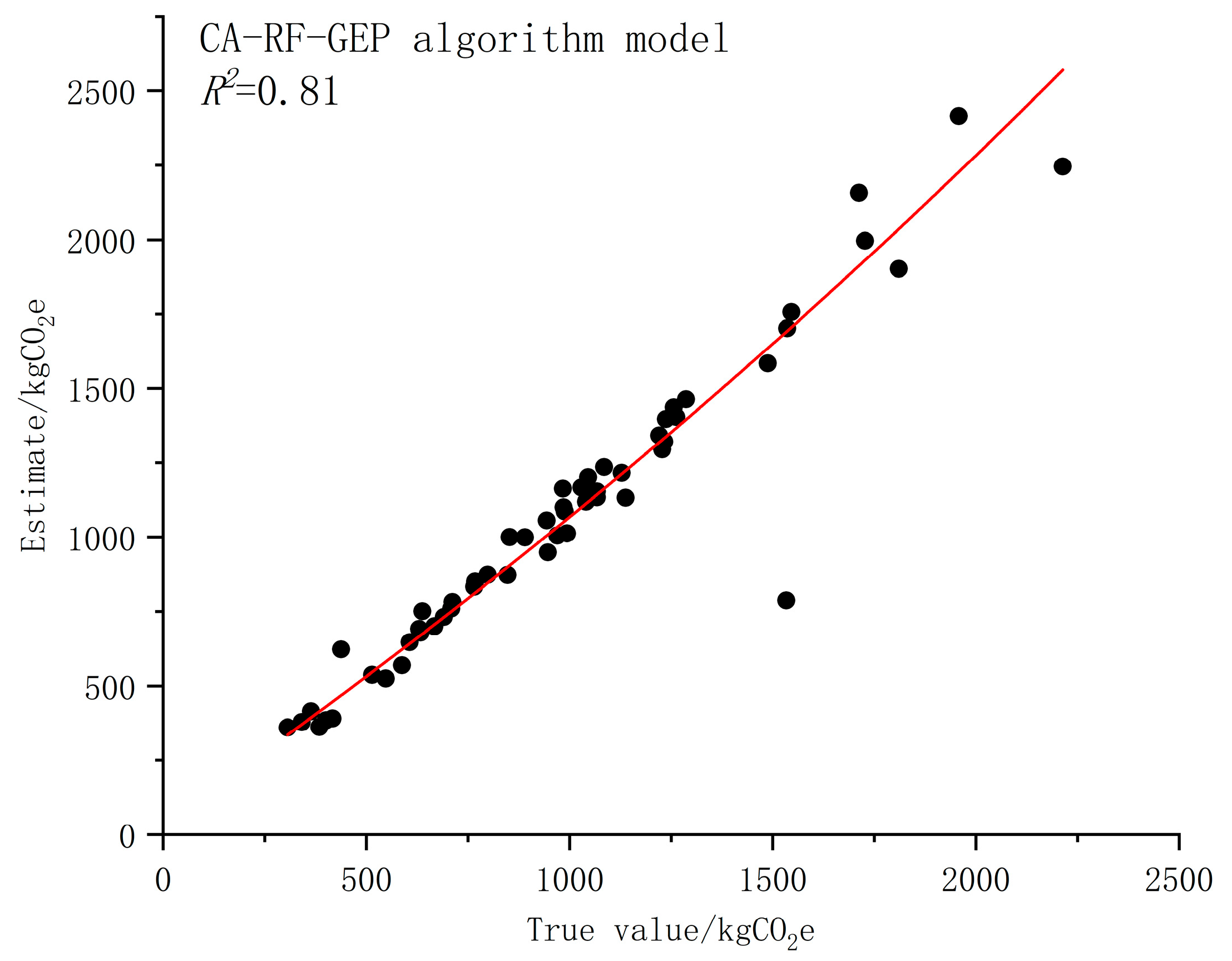
The experimental data visualization comparison (Figure 4) demonstrates the superior predictive accuracy of the GEP-based model. The coefficient of determination (R²) between predicted and observed carbon emission values reaches 0.81, indicating strong model-fitting capability. Key parameter analysis (Table 1) reveals that with a maximum sample deviation of 9674.68 kgCO₂e, the model maintains high-precision performance: RMSE: 156.13 kgCO₂e, MAE: 99.17 kgCO₂e.

Furthermore, both RRSE and MAPE converge below the 8% threshold, confirming consistent relative error control. Comprehensive error metric integration validates the predictive reliability of the CA–RF–GEP hybrid architecture through systematic multi-indicator error quantification.

4.3. Comparative Analysis with Other Models

Under identical experimental conditions and datasets, conventional GEP and BP neural network algorithms were employed to construct prediction models (specific parameter settings shown in

Table 12. Parameter setting of BP neural network model.

Parameter	Value
Number of Neurons in Hidden Layer 1	32
Dropout Rate after Hidden Layer 1	0.4
Number of Neurons in Hidden Layer 2	8
Dropout Rate after Hidden Layer 2	0.5
Number of Neurons in Output Layer	1
Maximum Training Epochs	2000
Batch Size	32
Number of Neurons in Hidden Layer 1	32

). Model accuracy metrics were independently calculated, with results presented in

Table 13. Comparison of model indicators.

Statistical Indicators	R2	RMSE	MAE	RRSE	MAPE
CA–RF–GEP Algorithm Model	0.81	156.13	99.17	0.16	9.4%
Traditional GEP algorithm model	0.44	682.00	271.04	0.87	25.63%
BP neural network algorithm model	0.74	394.44	219.72	0.50	19.73%

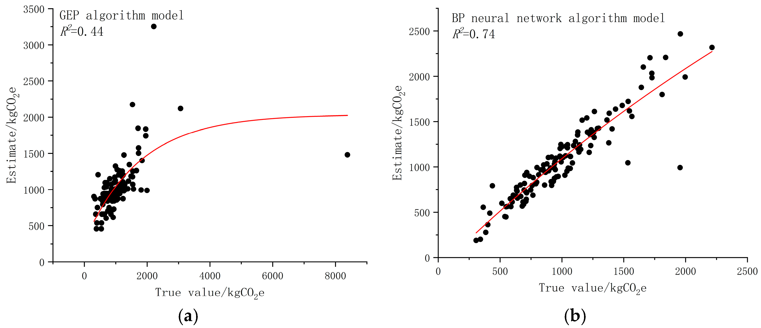
. Figure 5 plots the fitting curves for control groups a (GEP) and b (BP neural network), respectively.

Comparative analysis of Figure 4 and Figure 5a,b reveals close alignment between predicted and actual values for both the CA–RF–GEP hybrid model and BP neural network, demonstrating superior fitting performance over the traditional GEP model. Statistical metrics in Table 9 highlight limitations of traditional GEP: it considers only a subset of influencing factors while inadequately addressing data complexity and variability, resulting in compromised predictive accuracy.

Although both CA–RF–GEP and BP neural network employ multi-factor modeling frameworks, the former exhibits significant advantages in prediction accuracy and error control:

• Coefficient of Determination (R²): CA–RF–GEP achieves 0.81, improving by 3.8% over BP network (0.78).
• Root Mean Square Error (RMSE): 156.13 kgCO₂e for CA–RF–GEP, representing 42% reduction versus BP network.
• MAE/RRSE/MAPE: Optimized by >35% in CA–RF–GEP.
• Notably, under extreme samples with maximum deviation of 9674.68 kgCO₂e, the CA–RF–GEP model’s error metric integration value is merely one-third of traditional GEP. This demonstrates a tenfold performance difference, validating enhanced robustness and precision of the CA–RF–GEP architecture.

4.4. Low-Carbon Pathway Research

Guided by the three-tier weight structure, this section explores pathways for low-carbon urban transformation through multidimensional planning elements. By refining key domains—building facilities, transportation systems, spatial environments, and residential behaviors—we establish practical approaches to achieve carbon goals, providing systematic references for policymakers and urban planners.

4.4.1. Building Facility Carbon Reduction

1.

Energy Retrofit (Core Layer)

Power Distribution Upgrade: For areas with insufficient transformer capacity, implement flexible regulation schemes (Zhang et al. [18,19]) integrating PV-storage microgrids to optimize adjustable loads under safety constraints.

Renewable Integration: Adopt Germany’s PV subsidy model [20,21] for grid-fed surplus electricity and diversified products. Prioritize distributed PV with small-scale wind power in Baotou to enhance energy self-sufficiency.

2.

Building Envelope Retrofit (Buffer Layer)

Enclosure Reconstruction: Use high-efficiency insulation (EPS/rock wool boards), bridge-broken aluminum hollow glass windows, and external shading. Cold-region cases show 59.47% energy reduction and 33.95% life-cycle carbon cut (11.12% incremental cost) [22].

HVAC Optimization: Promote high-efficiency equipment (magnetic levitation chillers, ground/air-source heat pumps) with smart controls for >30% efficiency gains [23].

4.4.2. Transportation Carbon Reduction

1.

Short-term Strategy (Core)

Green Travel Promotion: Enhance slow-mobility systems (covered corridors + vertical transit), increase bus connectivity (community shuttles + dedicated lanes) to reduce elderly short-trip reliance.

Shared Mobility Management: Dynamically allocate shared bikes/e-vehicles to prevent idle resources.

2.

Long term strategy (buffer)

Energy Transition: Phase out high-carbon vehicles as EV penetration reaches 8.9% (2024).

4.4.3. Spatial Environment Optimization

1.

Microclimate Regulation (Buffer)

Wind Protection: Planting single-row 2 m trees 15 m leeward reduces wind speed by 30–40% (double-row: 50%) [24], minimizing winter heat loss; 1 °C summer temperature drop cuts AC energy use.

Carbon Sequestration: Prioritize native high-carbon-fixation species; vertical greening increases carbon storage by 25–40% [25].

2.

Environmental Engineering (Buffer)

Water Recycling: Rainwater cascade + MBR sewage reuse (>70% recovery) reduces municipal water demand.

Waste Treatment: Smart sorting + pneumatic transport cuts transport energy by 60%; methane recovery via anaerobic digestion.

4.4.4. Behavioral Activity Pathways (Periphery)

Habit Formation: Promote energy-saving appliances and non-essential power control through education and green credit incentives (e.g., energy-saving competitions).

15-Minute City: Mixed-use layouts reduce commuting needs and support local low-carbon supply chains (cutting logistics emissions).

Community Engagement: Regular interactive low-carbon workshops enhance resident participation.

4.5. Model Portability and Generalization Discussion

4.5.1. Model Portability

The proposed CA–RF–GEP hybrid model demonstrates robust performance in predicting household carbon emissions for aging residential communities under the arid-cold climatic conditions of Kundulun District, Baotou City, indicating significant application potential. Nevertheless, rigorous evaluation of its cross-regional portability and generalization capability across diverse geographical contexts and application scenarios is imperative. The model’s predictive accuracy remains highly contingent upon region-specific attributes embedded in the training data, with primary limitations manifesting in the following dimensions:

Climate Dependency: Key driving factors identified by the model—particularly heating energy consumption (X₁₇)—exhibit patterns and intensities intrinsically linked to arid-cold climates. Application to regions with vastly different climatic profiles (e.g., warm-humid or hot-humid zones) would fundamentally alter critical elements: Shift in dominant energy types (increased cooling energy share), Variations in energy intensity and Adjustments to heating season duration. The assigned weight for heating energy (0.05) and retrofit pathways derived therefrom (e.g., envelope upgrades, heat source optimization) demonstrate limited applicability in non-cold regions, directly compromising prediction accuracy.

Building and Demographic Specificity: Training data encapsulates Baotou-specific building attributes (e.g., construction year X₉, floor area X₁, envelope condition) and household demographics (e.g., elderly population proportion X₈) with associated energy-use patterns. Systematic variations exist across regions—exemplified by southern Chinese communities typically lacking centralized heating systems with distinct age distributions—necessitating further validation of the model’s adaptability to such divergences.

Regional Energy Structure and Policy Influence: Model predictions are contingent upon inputted regional grid emission factors (Table 4) and localized energy pricing policies (e.g., water pricing reform impacts on water consumption X₁₅, Section 4.1.2). Significant disparities in a target region’s electricity mix (e.g., renewable energy penetration), primary fossil fuel types, or energy policies will directly disrupt: Carbon calculation logic for associated variables (X₁₄, X₁₅, X₁₆, X₁₇) and the model’s fundamental input-output relationships.

Absence of Behavioral and Psychological Factors: The model currently does not incorporate parameters related to resident behavioral and psychological aspects (e.g., indoor thermal comfort preference settings, energy-saving awareness intensity, habits of using energy-consuming appliances). These factors are crucial causes of variations in carbon emissions between households at the micro level and may also form regional behavioral patterns at the macro level due to differences in local culture or socioeconomic status. Neglecting these factors limits the model’s ability to capture individual-level differences and cross-regional behavioral pattern changes, posing a challenge to its generalization accuracy.

Behavioral–Psychological Factor Omission: The model currently excludes resident behavioral–psychological parameters (e.g., thermal comfort preferences, energy-saving awareness, appliance usage patterns). These constitute critical micro-level variance drivers in household emissions and may manifest as macro-level regional behavioral patterns due to cultural/socioeconomic differences. This omission impedes Individual-level difference capture and Cross-regional behavioral transition tracking thereby compromising generalization accuracy.

4.5.2. Model Generalization Enhancement Pathways

To advance generalization capability, future work prioritizes:

Cross-Regional Validation and Calibration: Collect longitudinal data from aging communities across climate zones, city types, and development stages for cross-regional validation. Perform parameter adjustments/model restructuring based on results, establishing regional calibration coefficients to assess universality.

Behavioral-Socioeconomic Integration: Acquire variables on energy-use behaviors, conservation attitudes, and socioeconomic status via household surveys and smart meter analytics. Investigate incorporating these as supplementary inputs or developing hierarchical/clustered prediction models to enhance micro-level individual difference characterization and macro-level regional pattern capture.

Development of a Modular and Adaptive Learning Framework: Consider designing a modular model architecture that decouples the generalizable core algorithms (e.g., CA-based spatial denoising, RF feature selection, GEP optimization) from region-specific parameter/factor modules (e.g., climate sensitivity adjustment coefficients, localized energy carbon emission factor libraries, and typical energy use behavior pattern libraries). Explore leveraging transfer learning techniques to transfer knowledge acquired from training in arid and cold regions to models for new regions, reducing dependence on large amounts of labeled data for new areas and accelerating the model adaptation process.

Widespread model application necessitates rigorous region-specific validation/calibration and incorporation of comprehensive drivers—particularly behavioral variables. This constitutes the critical pathway for transitioning from case-specific models to broad-scenario deployment.

5. Conclusions

This study addressed the critical challenge of high-dimensional data modeling for predicting household carbon emissions in aging residential areas within arid cold regions by introducing and validating a novel CA–RF–GEP hybrid framework. The core contribution lies in its innovative methodological integration, demonstrating significant advancements:

Spatial Noise Mitigation: By explicitly simulating spatial interactions between households using Cellular Automata (CA), the model effectively quantified and suppressed noise interference arising from the heterogeneous degradation of building envelopes, achieving enhanced noise reduction efficiency. This provides a robust foundation for spatial analysis in complex urban environments.

Data-Driven Driver Identification: The integration of Random Forest (RF) enabled the rigorous identification and quantification of key emission drivers. Analysis identified electricity consumption (X₁₆, weight = 0.4329) and heating energy use (X₁₇, contribution to RMSE = 21%) as dominant factors, yielding crucial and actionable insights for targeted interventions.

Explainable and Accurate Prediction: Gene Expression Programming (GEP) achieved higher-precision carbon emission predictions compared to traditional methods (R² = 0.81, RMSE = 156.13 kgCO₂e), successfully balancing the competing demands of predictive capability and model interpretability.

Beyond its technical innovation, this framework serves as a robust decision-support tool for sustainable urban renewal. The identified drivers translate into specific, prioritized low-carbon retrofit pathways:

Electricity Optimization: Prioritize integrating photovoltaics and smart grid deployment to reshape consumption patterns.

Heating Decarbonization: Implement household-level heat metering combined with ground-source heat pump systems to address the significant emission burden associated with heating.

Spatially Targeted Strategies: Develop location-specific measures, such as differentiated wall insulation retrofits in high-emission zones (e.g., Kundulun District), leveraging the model’s spatial analysis capability for precision governance.

While demonstrating strong applicability in the case study of Kundulun District, Baotou, this study acknowledges limitations that highlight important directions for future research:

Scope and Dynamics: Validation relied on cross-sectional data from a single climatic zone. Future work must incorporate longitudinal datasets across diverse climatic regions to rigorously assess the model’s temporal robustness, its ability to capture dynamic trends (e.g., retrofit effects, behavioral shifts), and its broader geographical transferability.

Human Dimension: The current exclusion of behavioral psychology parameters (e.g., heating temperature preferences, appliance usage habits) constitutes a key limitation, potentially underestimating interpersonal variation and the socio-behavioral complexity of emission reduction. Integrating Multi-Agent Simulation (MAS) is a critical next step to explicitly model the dynamic interactions between heterogeneous households (agents), the built environment, evolving policies, and environmental factors. This will yield a more comprehensive understanding of intervention impacts and social feasibility.

In conclusion, the CA–RF–GEP framework represents a significant step forward in quantitative, spatially explicit modeling of urban carbon emissions. It offers a novel, integrated approach to overcome high-dimensionality challenges, generating insights that are both accurate and interpretable. This research not only provides a practical tool for designing effective, spatially tailored decarbonization strategies in aging communities but also establishes a methodological foundation for future exploration of the complex, multi-scale dynamics within human-building-environment systems towards achieving urban sustainability and climate goals. Future enhancements focusing on temporal dynamics and human behavior integration will further increase the framework’s utility for policy simulation and evaluation.

References

- State Council of the PRC. 2024–2025 Action Plan for Energy Conservation and Carbon Reduction. Available online: https://www.gov.cn/zhengce/content/202405/content_6954322.htm (accessed on 18 April 2025).
- Xia, C.; Zheng, H.; Meng, J.; Shan, Y.; Liang, X.; Li, J.; Yin, Z.; Chen, M.; Du, P.; Wang, C. Outsourced carbon mitigation efforts of Chinese cities from 2012 to 2017. Nat. Cities 2024, 1, 480–488. [Google Scholar] [CrossRef]
- Tian, H.; Wang, W.; Hao, T. Grid-Based Characterization and Sustainable Planning for Fractured Urban Textures: A Case Study of Nanhao Village in Baotou. Buildings 2024, 15, 5. [Google Scholar] [CrossRef]
- Hu, Y.; Zhang, Y.; Xia, X.; Li, Q.; Ji, Y.; Wang, R.; Li, Y.; Zhang, Y. Research on the evaluation of the livability of outdoor space in old residential areas based on the AHP and fuzzy comprehensive evaluation: A case study of Suzhou city, China. J. Asian Archit. Build. Eng. 2024, 23, 1808–1825. [Google Scholar] [CrossRef]
- JetBrains. PyCharm, Version 2023.1.4—Community Edition; JetBrains: Prague, Czech Republic, 2023. Available online: https://www.jetbrains.com/pycharm/ (accessed on 5 May 2025).
- Alzara, M.; Rehman, M.F.; Farooq, F.; Ali, M.; Beshr, A.A.A.; Yosri, A.M.; A El Sayed, S.B. Prediction of Building Energy Performance Using Mathematical Gene-Expression Programming for a Selected Region of Dry-Summer Climate. Eng. Appl. Artif. Intell. 2023, 126, 106958. [Google Scholar] [CrossRef]
- Iqbal, M.F.; Liu, Q.-F.; Azim, I.; Zhu, X.; Yang, J.; Javed, M.F.; Rauf, M. Prediction of mechanical properties of green concrete incorporating waste foundry sand based on gene expression programming. J. Hazard. Mater. 2020, 384, 121322. [Google Scholar] [CrossRef]
- Li, S.; Tong, Z.; Haroon, M. Estimation of transport CO2 emissions using machine learning algorithm. Transp. Res. Part D Transp. Environ. 2024, 133, 104276. [Google Scholar] [CrossRef]
- Chen, Z. High-Efficiency Cooling Source Design Practice for Data Centers Based on Independent Temperature and Humidity Control. Build. Energy Effic. 2023, 51, 79–83, (In Chinese and English). [Google Scholar]
- Hu, X.; Li, Z.; Cai, Y.; Wu, F. Urban construction land demand prediction and spatial pattern simulation under carbon peak and neutrality goals: A case study of Guangzhou, China. J. Geogr. Sci. 2022, 32, 2251–2270. [Google Scholar] [CrossRef]
- GB/T 2589-2008; General Rules for Calculation of the Comprehensive Energy Consumption. Standards Press of China: Beijing, China, 2008.
- GB/T 51366-2019; Standard for Building Carbon Emission Calculation. China Architecture & Building Press: Beijing, China, 2019.
- Kaur, J.; Bala, A. A hybrid energy management approach for home appliances using climatic forecasting. Build. Simul. 2019, 12, 1033–1045. [Google Scholar] [CrossRef]
- Xiang, J.; Liu, H.; Li, X.; Jones, P.; Perisoglou, E. Multi-Objective Optimization of Ultra-Low Energy Housing in Hot Summer Cold Winter Climate Zone of China Based on a Probabilistic Behavioral Model. Buildings 2023, 13, 1172. [Google Scholar] [CrossRef]
- Luo, W.; Liu, W.; Liu, W.; Xia, L.; Zheng, J.; Liu, Y. Analysis of influencing factors and carbon emission scenario prediction during building operation stage. Energy 2025, 316, 134401. [Google Scholar] [CrossRef]
- Exhaust Gas Turns into New Energy, Carbon Reduction Has a ‘Good Prescription’—Exploration of Green and Low-Carbon Development Path by Orchid Group’s Research on Low-Concentration Coal Mine Methane Utilization Technology. Jincheng News, 18 April 2025. Available online: https://www.jcgov.gov.cn/dtxx/jcdt/202504/t20250416_2130071.shtml (accessed on 21 May 2025).
- Guo, S.; Li, A. Typical Practices and Suggestions for Water Supply Price Reform of Water Conservancy Projects in Shandong Province. Water Resour. Dev. Res. 2020, 30, 21–23+39. [Google Scholar] [CrossRef]
- Yang, S.; Cho, H.M.; Yun, B.Y.; Hong, T.; Kim, S. Energy usage and cost analysis of passive thermal retrofits for low-rise residential buildings in Seoul. Renew. Sustain. Energy Rev. 2021, 151, 111617. [Google Scholar] [CrossRef]
- Liang, Z.; Li, X.; Guo, L.; Zhang, J. Insights from Germany’s Power System Transformation on the Development and Operation of New Energy in China. Autom. Electr. Power Syst. 2024, 48, 2884–2894. [Google Scholar] [CrossRef]
- Lee, J.; Shepley, M.M. Benefits of solar photovoltaic systems for low-income families in social housing of Korea: Renewable energy applications as solutions to energy poverty. J. Build. Eng. 2020, 28, 101016. [Google Scholar] [CrossRef]
- Wang, G.; Li, X. Comprehensive Optimization of Low-Carbon Buildings Integrating Phase Change Walls and Photovoltaics. Heat. Vent. Air Cond. 2025, 55, 112–118. [Google Scholar] [CrossRef]
- Li, H.X.; Wang, S.W. Coordinated optimal design of zero/low energy buildings and their energy systems based on multi-stage design optimization. Energy 2019, 189, 116202. [Google Scholar] [CrossRef]
- Karali, N.; Shah, N.; Park, W.Y.; Khanna, N.; Ding, C.; Lin, J.; Zhou, N. Improving the energy efficiency of room air conditioners in China: Costs and benefits. Appl. Energy 2020, 258, 114023. [Google Scholar] [CrossRef]
- Li, X.; Tang, H. Research on the Impact of Outdoor Trees Based on Sustainable Energy Management on Pedestrian Wind and Thermal Environment around Preschool Education Buildings. J. Cent. South Univ. 2024, 31, 2039–2053. [Google Scholar] [CrossRef]
- Chen, R.; Fu, X. Simulation study on plant improvement of wind environment in old residential streets. Urban. Archit. 2022, 19, 190–194. [Google Scholar] [CrossRef]
Figure 1.
Chromosome encoding method. The chromosome consists of 8 genes (positions 0–7) storing symbolic representations of mathematical operations and variables. The expression is encoded as the sequence: Q (square root function), + (addition operator), * (multiplication operator), * (multiplication operator), a, b, c, c. Note: The asterisk explicitly denotes the multiplication operator in the encoded sequence.
Figure 2.
Survey on the distribution map of residential area samples.
Figure 3.
Flow chart of CA–RF–GEP hybrid algorithm.
Figure 4.
Fitting diagram of CA–RF–GEP model.
Figure 5.
(a) Fitting diagram of traditional GEP algorithm model figure. (b) Fitting diagram of BP neural network algorithm model figure.