Voxel Interpolation of Geotechnical Properties and Soil Classification Based on Empirical Bayesian Kriging and Best-Fit Convergence Function

Abstract

To support bearing capacity estimates, this study develops and tests a geoprocessing workflow for predicting soil properties using Empirical Bayesian Kriging 3D and a classification function. The model covers a 183 m × 185 m × 24 m site in Astana (Kazakhstan), based on 16 boreholes (15–24 m deep) and 77 samples. Eight geotechnical properties were mapped in 3D voxel models (812,520 voxels at 1 m × 1 m × 1 m resolution): cohesion (c), friction angle (φ), deformation modulus (E), plasticity index (PI), liquidity index (LI), porosity (e), particle size (PS), and particle size distribution (PSD). Stratification patterns were revealed with ~35% variability. Maximum φ (34.9°), E (36.6 MPa), and PS (1.29 mm) occurred at 8–16 m; c (33.1 kPa) and PSD peaked below 16 m, while PI and e were elevated in the upper and lower strata. Strong correlations emerged in pairs φ-E-PS (0.91) and PI-e (0.95). Classification identified 10 soil types, including one absent in borehole data, indicating the workflow’s capacity to detect hidden lithologies. Predicted fractions of loams (51.99%), sandy loams (22.24%), and sands (25.77%) matched borehole data (52%, 26%, 22%). Adjacency analysis of 2,394,873 voxel pairs showed homogeneous zones in gravel–sandy soils (28%) and stiff loams (21.75%). The workflow accounts for lateral and vertical heterogeneity, reduces subjectivity, and is recommended for digital subsurface 3D mapping and construction design optimization.

1. Introduction

The basis of information on soils is an engineering–geological report containing data obtained in field and laboratory conditions, including testing of samples [1]. Subsequently, these data are used to assess the bearing capacity of the base [2]. Geotechnical surveys often provide discrete property values from sparse borehole data, which may fail to capture subsurface variability [3,4]. 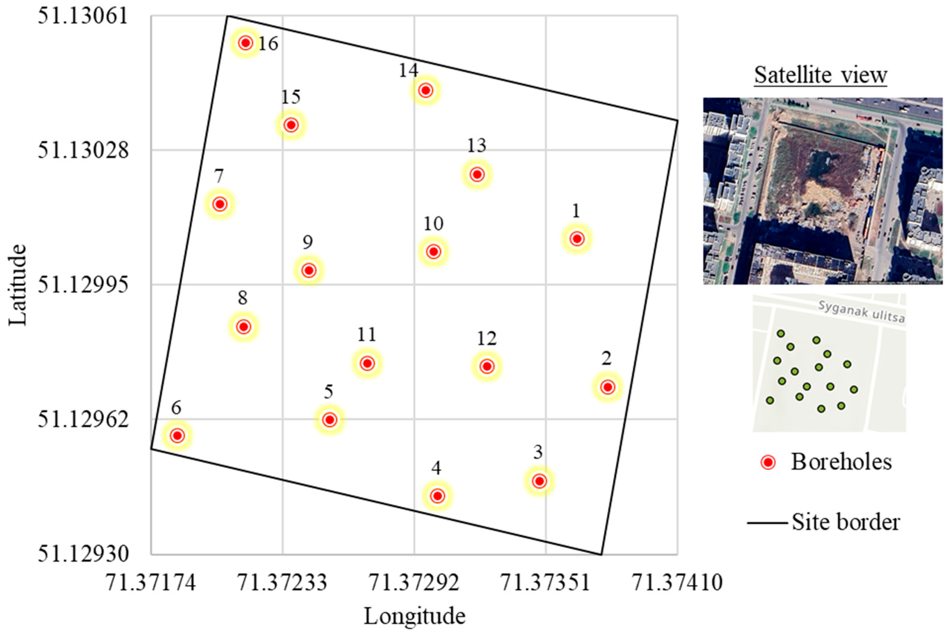When data are needed at unknown locations between boreholes [3], geotechnical engineers and designers rely on the recommendations of regulations that specify soil properties for an idealized state [5]. In areas with complex lithology, such as clayey soils in Astana (Kazakhstan), traditional reliance on normative tables can lead to oversimplification and design uncertainty, failing to reflect local variability critical for structural safety [6,7].

Current solutions [8] for automated estimates are based on 2D or 3D modeling and finite element calculations, where the input data are empirical parameters from a geotechnical report [9]. The amount of input data contributes to the realism of the base model and the reliability of the results of the calculation of its bearing capacity [10,11].

In recent decades, the need for a more complete picture of soil occurrence and its physical and mechanical characteristics has increased significantly, as accidents in buildings and facilities related to base settlement and waterlogging have become more frequent [12,13]. This has contributed to unlocking the potential of alternative techniques and tools to represent the geological structure and spatial distribution of soil properties [14]. The latter has been widely applied in soil science. Soil maps and digital elevation models are created using Geographic Information Systems (GISs) [15]. The model using these units assumes that the mapped soil property is homogeneous within a certain zoned classification, and changes occur only outside the zone, which is not quite similar to the natural pattern of occurrence [16], since it should be taken into account that soil properties have a continuous character of distribution, and though smoothly, they do change in space [17]. Although widely used [18,19,20,21,22,23,24,25,26,27,28,29,30], traditional 2D interpolation methods like Kriging, IDW, Topo to Raster, Natural Neighbor, and Spline often fail to capture vertical continuity and complex soil stratigraphy [31,32,33,34]. More accurate distribution requires 3D interpolation based on non-traditional primitives such as voxels [35,36]. However, the input of geotechnical soil properties into voxel layers is a rather labor-intensive process, feasible only when using special algorithms. There is not much research in this direction. For example, [37] created an algorithm for regular voxel separation based on layered interpolation data, which improves the accuracy and efficiency of geologic modeling. The study [38] presents a geological data model using BIM and GIS for 3D modeling and geological information management, incorporating important geometric, semantic, and spatial information and applying boundary and voxel representation. In [39], the differences between the stratum modeling approach using stratigraphically ordered surfaces and the voxel modeling approach based on a structured grid of volumetric pixels were analyzed to evaluate their impact on groundwater model predictions. The authors of [40] proposed a 3D geotechnical spatial modeling technique for borehole datasets using optimization of geostatistical approaches. This study improves the design of large-span bridge supports by statistically processing geotechnical data in unexplored regions. The study [41] proposes a method for voxel-based modeling of geotechnical properties of urban areas using Natural Neighbor interpolation with a large number of borehole logs. The method aims to construct 3D voxel models of the geologic section by summarizing horizontal two-dimensional grid data. This approach improves geologic analysis and facilitates the use of open borehole logs in urban areas, contributing to effective urban infrastructure planning and disaster risk assessment. In [42], an extended octo-tree-based framework for comprehensive geotechnical analysis integrating geologic, microseismic, and change detection data based on Mobile Laser Scanning is presented. This approach includes efficient change detection methods based on statistical derivations and additional octo-tree data structures that provide voxel-level data integration and linking, semantic clustering, and comprehensive geotechnical analysis.

Previous voxel-based modeling studies [37,38,41] have demonstrated the value of 3D gridded representations for subsurface visualization and have incorporated parameters such as grain size, resistivity, or porosity to infer lithological variation. However, these approaches often do not include core geotechnical parameters such as cohesion, friction angle, or deformation modulus, which are critical for engineering decision-making. Moreover, voxel assignments in prior works are typically based on visual or qualitative thresholds rather than formal classification functions. Some studies, such as [39], have focused on hydrogeological applications, while others [40] emphasized spatial visualization using GIS tools. Although these models offer useful insights, they do not support automated geotechnical classification across multiple parameters. Additionally, many existing voxel workflows require extensive manual preprocessing, iterative parameter tuning, or expert judgment to tailor models to specific sites [42], limiting scalability and reproducibility. Thus, while voxel-based 3D models have emerged as powerful tools for subsurface representation, many rely on limited parameters, manual classification, or high computational demands, limiting their applicability in routine geotechnical workflows.

This paper introduces a geoprocessing workflow that integrates Empirical Bayesian Kriging 3D (EBK 3D) [43,44] with a convergence-based classification function. The method interpolates eight geotechnical properties of soils between boreholes (hereinafter—intermediate soil properties (ISPs)) and automatically assigns soil types in voxel space, enhancing the manual characterization of [7]. Unlike previous studies that focus on either geometric modeling or interpolation of individual soil properties, this approach combines multi-parameter 3D interpolation with rule-based classification, providing more realistic stratification and reducing subjectivity. The method enables the detection of unrecorded lithological zones and reproduces soil type proportions similar to field data. Implemented in ArcGIS ModelBuilder, the workflow is replicable and scalable.

2. Materials and Methods

2.1. Data Collection and Preparation

For modeling the workflow that allows for determining the ISP, the data of engineering–geological surveys at the site (Figure 1) of construction of an apartment complex in Astana (Kazakhstan), obtained from Geocenter Astana, LLP [45], were taken as initial data.

The construction site has a rectangular shape with layout dimensions of about 130 m × 130 m. On the site, 16 boreholes were drilled at different points, the coordinates of which were pre-determined by geodesic equipment. The boreholes were drilled to certain depths, from which soil cores were extracted, and the capacities (thicknesses) of engineering–geological elements (EGEs) were determined according to visual–lithological boundaries of changes in soil composition and condition (Figure 2) in accordance with ISO 14688–1 [46].

The diagram in Figure 2 presents the stratigraphic characterization of the 16 boreholes drilled in the study area. In order to cover weak and compressible soils of the construction site base, the boreholes were drilled at depths from 15 to 24 m. In this case, boreholes No. 1–10 are 18 m deep, boreholes No. 11–12 are 15 m deep, and boreholes No. 13–16 are 24 m deep. The dashed intervals in the columns of the diagram correspond to the thicknesses of different EGEs, of which there are 9 in total. According to visual and manual identification per ISO 14688-1 [46] and preliminary classification per ISO 14688-2 [47], the stratigraphic structure of the EGE is characterized by pronounced lateral and vertical heterogeneity of layer thicknesses, which indicates a complex lithogenic history of the groundmass formation. In the upper part of the sections, loosened and weakly compacted soils prevail, being replaced with depth by denser soils of different nature. To establish the geotechnical properties of the soils (

Table 1. Borehole data from the study area. Adapted with permission from [45], Geocenter Astana, LLP, 2023.

EGE	Samples	Soil Type (Consistency)	Range of Values of Geotechnical Properties in EGEs
			Cohesion, c [kPa]	Friction Angle, φ [°]	Deformation Modulus, E [MPa]	Plasticity Index, PI [%]	Liquidity Index, LI	Void Ratio, e	Particle Size, PS [mm]	Particle Size Distribution, PSD [%]
1	1	Bulk loam (hard to soft plastic)	-	-	4.5	9.1	−0.49	0,537	-	-
2	8	Loam (soft plastic to fluid)	-	-	1.3	10.6 to 16.9	−1.14 to 2.03	1.286 to 2.9	-	-
3	18	Loam (hard to fluid)	20 to 33	12.5 to 13.9	3.3 to 4.3	7.8 to 15	−0.68 to 1.1	0.613 to 1.248	-	-
4	11	Sandy loam (hard to fluid)	17 to 23	18.9 to 21.8	7.5 to 9.5	4 to 6.7	−0.42 to 1.79	0.467 to 0.824	-	-
5	7	Medium sand	-	33 to 34	-	-	-	-	0.5 to 2	56.5 to 68.1
6	5	Gravelly sand	-	32 to 33	-	-	-	-	>2	26.7 to 37.5
7	9	Sandy loam (plastic to fluid)	17	26.2	12.4 to 17.3	3.7 to 5.5	−1.52 to 1.13	0.862 to 1.045	-	-
8	13	Loam (hard to tightened plastic)	27 to 60	20.6 to 22.9	12.4 to 16.5	7.5 to 12.9	−0.76 to 1.81	0.615 to 1.221	-	-
9	5	Silt (hard to plastic)	-	-	-	3.1 to 9.7	−1.99 to 0.24	-	>2	50.8 to 63.4

), core samples were taken at different depths (about the middle of each EGE layer) and tested in field and laboratory conditions [45].

According to Table 1, a total of 77 samples were collected. The final classification according to [48] based on the values of geotechnical properties revealed that the most common soil type at the base of the site is loam of different consistencies, found in 52% of the samples (39 pieces). In 26% of the samples (20 pieces), sandy loam of varying consistencies was found. In the remaining 22% of the samples (18 pieces), sandy soils, including silt, were detected. The table also lists the ranges of values for the major geotechnical properties for each EGE.

In the process of preparing the data for use in building the voxel model and conducting spatial analysis, the EGE data were loaded into template

Table 2. Template of soil properties data from boreholes.

Sample No.	Latitude, Lat [°]	Longitude, Lon [°]	Depth, d [m]	Soil Property, Pi [*]
1	Lat1	Lon1	d1	Pi,1
…	…	…	…	…
N	LatN	LonN	d1	Pi,N

* The measurement unit depends on the considered soil property.

, from which, in turn, an initial geospatial database with a .gdb extension (I-GDB) was generated in ArcGIS Pro 3.5 software.

I-GDB was designed for the input of spatially referenced borehole data and its connection to the developed geoprocessing workflow. Geographic coordinates (latitude and longitude in the WGS 1984 UTM Zone 42N coordinate system), soil sampling depth (d), and geotechnical soil properties (P_i) such as cohesion (c), friction angle (φ), deformation modulus (E), plasticity index (PI), liquidity index (LI), porosity (e), particle size (PS), and particle size distribution (PSD) are entered into the I-GDB for each borehole. The I-GDB included 77 samples from 16 boreholes within a 135 m × 135 m × 24 m site, which represents a typical sampling density for geotechnical surveys at this scale. In practice, it is common for certain properties to be missing in some samples, as the selection of laboratory tests is often determined by the specific needs and budget of the project. In our case, a small number of samples lacked values for properties such as PI, LI, and e. To ensure consistent input for voxel classification, these missing values were supplemented using normative values derived from [7]. This approach reflects standard engineering–geological practice, where reliance on normative values in the absence of specific test results is widely accepted. When applied appropriately, such substitution does not compromise the validity of the analysis, particularly when the goal is to produce spatial generalizations through interpolation. It enables the geoprocessing workflow to proceed effectively without introducing significant bias, since the interpolated values between boreholes remain based on observed data.

2.2. Modelling the Geoprocessing Workflow

Modeling of the geoprocessing workflow was performed in the ArcGIS Pro 3.5 model builder using the built-in ArcToolbox toolkit. The workflow runs on a personal computer (PC)—ASUS Zenbook 14 Flip UP3404VA (ASUSTeK Computer Inc., Taipei, Taiwan) ultrabook equipped with an Intel Core i7-1360P processor (2.2 GHz), 16 GB RAM, 1 TB SSD, and Intel Iris Xe graphics, and Windows 11 operating system. A key tool integrated into the workflow is EBK 3D [43], which was used to interpolate the ISP based on known well data from I-GDB. An important step in the design of the workflow was the establishment of the boundaries of the modeled area (Extent), for which 4 control points were set to delineate a rectangle of 183 m × 185 m (the dimensions of the voxel model in plan), with sides about 20 m away from the sides of the construction site to minimize the effect of the interface on the property values within the area during interpolation. When setting up EBK 3D, the following parameters from

Table 3. Parameters set in EBK 3D.

Parameter	Value	Notes
Input features	I-GDB	Initial geodatabase containing borehole data
Elevation field, m	d	Depth of sampling
Value field	Pi	i-th geotechnical property
Output	GL	Geostatic layer for further analysis and visualization
Semivariogram model type	Exponential	Suitable for subsurface conditions
Transformation type	Log empirical, except IL	IL may have negative values, so the transportation type None was set for it
Subset size	100	Appropriate for a medium-sized study area
Overlap	1	Ensures smoother transitions
Number of simulations	100	Ensures semivariogram stability
Order of trend removal	None
Search neighborhood	Standard 3D	Captures neighboring points in all directions
Max neighborhood	2	Captures spatial variability while avoiding over-smoothing
Min neighborhood	1	Ensures statistical reliability while avoiding interpolation gaps
Output surface type	Prediction	Represents the predicted geotechnical properties

were set.

The EBK 3D parameters in Table 3 were selected based on recommendations in the ArcGIS Pro documentation [44] and iterative testing on the dataset. The exponential semivariogram model was chosen due to the smooth spatial variation typically observed in subsurface conditions. A subset size of 100 provided a balance between computational efficiency and model stability, while an overlap of 1 ensured continuity across blocks. The number of simulations of 100 and the use of the “Standard 3D” neighborhood were set to maintain isotropy and minimize artifacts. The maximum and minimum neighborhood settings (2 and 1) ensured that interpolation included nearby observations without overfitting. Transformation type was set to “Log Empirical” for all properties except LI, which contains negative values.

The output data from EBK 3D were so-called spatial geostatic layers (GL) [44] for each of the input soil properties (P_i). These were used to produce multidimensional arrays by converting them via the GA Layer 3D To NetCDF tool [49] into a NetCDF file with the extension .nc. In this tool, the voxel resolutions in the X, Y, and Z axes are set to be equal to 1 m in order to correctly discretize the model. To visualize these NetCDF multidimensional arrays in a voxel representation, the Create Voxel Scene Layer Content tool was used to generate full 3D voxel models (Figure 3). During the modeling process, NetCDF files containing Pi were loaded, visualization parameters (color, transparency, range of values) were adjusted, and then the models were saved in Esri Scene Layer Package format with a .slpk extension.

Figure 3 shows the visualization of the model fragment made of voxels (Vs), each of which can also be represented as a pixel at a horizontal slice at a certain depth, and the entire medium plane as a raster image [50]. The fragment scheme demonstrates the principle of discretization of the subsurface space, in which it is divided into three-dimensional elements (i.e., voxels) with well-defined local coordinates (x, y, z). At the same time, each voxel contains the value of the predicted geotechnical property (P_i), and the full model allows for spatial statistical analysis of the distribution of soil properties in plane and depth, thus providing a more detailed view of the EGE structure. For such statistical analysis, we applied Box Plot, standard deviation, mean values, coefficients of variation, and correlation analysis.

The next step was the integration of a soil classification tool into the workflow, the task of which is to recognize whether a voxel belongs to a particular soil type (i.e., to assign a soil type). In survey practice, this procedure is performed manually by geotechnical engineers, guided by standards containing normative values of the main geotechnical properties of soils, such as those given in [7]. This standard contains conditions (

Table 4. Properties of clayey non-loess and Quaternary sandy soils [7].

Ordinal Number (n) and Name		$\mathbf{Ordinal} \mathbf{Number} \left(\mathit{i}\right), \mathbf{Name}, \mathbf{and} \mathbf{Average} * \mathbf{Values} \left(\overline{{\mathit{P}}_{\mathit{i},\mathit{s}}}\right)$
		1	2	3	4	5	6	7	8
n	Name	Cohesion, c [kPa]	Friction Angle, φ [°]	Deformation Modulus, E [MPa]	Plasticity Index, PI [%]	Liquidity Index, LI	Void Ratio, e	Particle Size, PS [mm]	Particle Size Distribution, PSD [%]
Clayey (Including Sandy Loam **) Soils
1	Sandy loam (hard)	17	27	19.5	4	0	0.525	-	-
2	Sandy loam (plastic)	17	27	19.5	4	0.5	0.525	-	-
3	Sandy loam (fluid)	14	23	19.5	4	1	0.525	-	-
4	Loam (hard)	33	23	22.5	12	0	0.525	-	-
5	Loam (semi-hard)	33	23	22.5	12	0.125	0.525	-	-
6	Loam (tightened plastic)	27	20.5	20	12	0.375	0.525	-	-
7	Loam (soft plastic)	18.5	15.5	11	12	0.625	0.525	-	-
8	Loam (fluid plastic)	18.5	15.5	11	12	0.875	0.525	-	-
9	Loam (fluid)	18.5	15.5	11	12	1	0.525	-	-
10	Clay (hard)	58.5	17.5	20	17	0	0.525	-	-
11	Clay (semi-hard)	58.5	17.5	20	17	0.125	0.525	-	-
12	Clay (tightened plastic)	44.5	14.5	15	17	0.375	0.525	-	-
13	Clay (soft plastic)	37	11	11	17	0.625	0.525	-	-
14	Clay (fluid plastic)	37	11	11	17	0.875	0.525	-	-
15	Clay (fluid)	37	11	11	17	1	0.525	-	-
Sandy soils
16	Gravelly and coarse sand	1.5	40.5	40	-	-	-	2	25
17	Medium coarse sand	2	37.5	40	-	-	-	1.25	50
18	Fine sand	4	33	33	-	-	-	0.375	75
19	Silty sand	5	31	25	-	-	-	0.25	75

* The average is taken between the range of values for each type of soil given in [7]. ** Sandy loam is a type of soil in which sand predominates, but it also contains enough silt and clay to exhibit plasticity. According to [7], sandy loam in non-loess Quaternary deposits is classified as a clayey soil due to its non-zero plasticity index (PI > 0), which distinguishes it from sands.

), which allow the recognition of the type by physical and mechanical properties of clayey non-loess soils and sands of Quaternary sediments, to which the soils at the base of the considered site (Figure 1) belong. It should be emphasized that this developed classification tool can also be adapted to other soil classification standards by replacing Table 4.

Table 4 above was integrated into the classification tool, which contains a special best-fit function (Equation (1)), which estimates the degree to which a voxel belongs to one of the 19 soil types listed in this table, depending on the P_i value contained in it.

$$\underset{1\le n\le 19}{\min }{D}_n={\sum }_{i=1}^m\left|\overline{P_{i,s}}-P_i\right|,$$

(1)

where n—ordinal number of soil type; i—ordinal number of soil property; m—possible number of considered soil properties (depends on the standard; in this case m = 8 [7]); $\overline{P_{i,s}}$—average of the standard value of soil property; P_i—value of an i-th soil property; D_n—discrepancy value.

The classification function (Equation (1)) calculates a discrepancy value (D_n) for each voxel by comparing its interpolated soil property values (P_i) with the average normative values for each soil type (Table 4) provided in [7]. The function applies a multivariate Euclidean distance approach [51]: the voxel is assigned to the soil type with the lowest total discrepancy across m properties. This approach allows consistent classification across all voxels using a rule-based, quantitative method rather than manual visual matching, as done in traditional borehole logging [7].

The classification resulted in a single 3D model of voxels, each containing the sequence number of one of the 19 soil types from Table 4. This model allowed us to evaluate the distribution of soil types in the plane and depth, as well as the layering and transitions from one soil type to another. The latter was assessed by visual–quantitative analysis, by counting the number of voxels attributable to each soil type both by depth and overall and visualized by diagrams.

Additional analysis was performed in order to identify the patterns of stratification and transition from one soil type to another within the extent of the investigated base. For this purpose, all values of soil types and the coordinates of their corresponding voxels (1 m × 1 m × 1 m in size) were exported in tabular form, based on which a spatial analysis of nearest neighbors was performed. Each voxel was matched with six potential neighbors along the ±x, ±y, and ±z directions (along the common sides). Within a model of size 183 m × 185 m × 24 m including 812,520 voxels, the maximum number of possible neighboring voxel pairs (i.e., unique adjacencies) was (183 − 1) × 185 × 24 + 183 × (185 − 1) × 24 + 183 × 185 × (24 − 1) = 2,394,873. In the process of analysis, all actually existing neighbors of each voxel were taken into account, and for each pair, the types of contacting soils were recorded. The result was a symmetric adjacency matrix in which diagonal elements represent the number of contacts between voxels of the same type (internal homogeneity), and non-diagonal elements represent the number of contacts between different soil types (boundaries and zones of lithologic transitions). The total sum of values in the matrix was 4,789,746, which is twice the number of unique neighboring pairs of voxels because each pair is counted twice, from the first to the second voxel and vice versa. To obtain the number of unique neighboring pairs of voxels, the values in the matrix were reduced to half scale. The obtained matrix allowed for visualization and quantification of the degree of heterogeneity of the soil base, as well as revealing the patterns of their natural–historical occurrence.

Validation of workflow performance was performed by comparing the EBK 3D interpolated values of soil properties with those obtained from borehole data for all 77 samples. Various statistical methods of deviation analysis were applied.

3. Results and Discussion

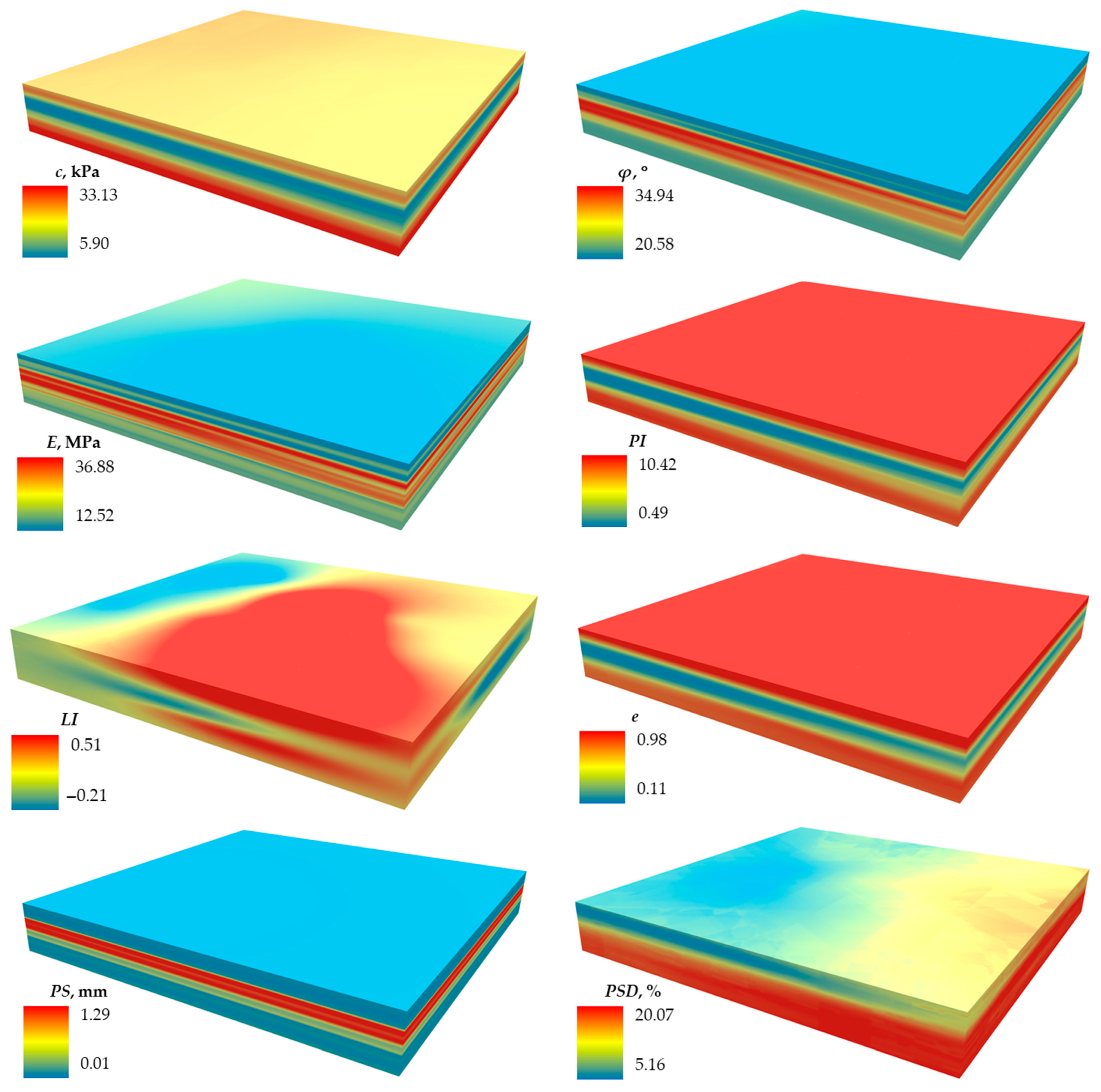
Figure 4 shows the 3D voxel models, with dimensions of 183 m × 185 m × 24 m, respectively containing 812,520 voxels with predicted values of eight base soil properties, including c, φ, E, PI, LI, e, PS, and PSD.

For the voxel models shown in Figure 4 above, gradient coloring from blue to red has been applied, denoting according to the indicated legends the lower and upper limits of soil property values, respectively, including c values—from 5. 9 to 33.12 kPa; φ—from 20.58 to 34.94; E—from 12.52 to 36.58 MPa; PI—from 0.49 to 10.42; LI—from −0.21 to 0.51; e—from 0.11 to 0.98; PS—from 0.01 to 1.29 mm; and PSD—from 5.16 to 20.07%. It is noteworthy that the values are slightly different from those originally set in the model from filled Table 2. However, the general trend is maintained, e.g., regarding LI, negative values are found in both cases. There is also a certain layering of close values by depth, repeating the layering trend of the soils themselves. The color gradient of the models shows that higher values are concentrated at an average depth of about 8–16 m for φ, E, and PS. For c and PSD, high values are located in the lower layers deeper than 16 m, and for PI and e, simultaneously in the upper (up to 7 m depth) and lower (below 16 m) layers. Low values of most properties alternate in opposite depth layers with small intervals of layers with average values. LI values, unlike values of all other properties, are not so subordinate to the layering trend. Apparently, the presence of negative values played a role here. The visual trend of LI values can be described as unevenly blurred both in depth and in plane. Thus, we can reasonably consider that the EBK 3D method applied for interpolation largely outperforms its classical predecessors applied in [18,19], such as Natural Neighbor, IDW, and Ordinary Kriging, by offering a detailed picture of the distribution of phenomenon properties in 3D space. Although these classical methods have been successfully applied to IPS prediction [31,32,33,34], the advantage of the proposed workflow is obvious (i.e., not just the EBK 3D method itself and the specifics of its reconfiguration (Table 3), but also the special soil classification function)—it considers the influence of properties in both plane and depth simultaneously. It should be emphasized that in this work only the basic eight soil properties (c, φ, E, PI, LI, e, PS, and PSD) were predicted, which did not include e.g., hydro-physical soil properties (moisture, organic carbon content, or superfine particles less than 10⁻³ m) as in [28,29]. However, the proposed workflow is quite capable of doing this, e.g., by increasing the interpolation resolution from 1 m to 10⁻³ m. However, a more powerful PC or server may be needed.

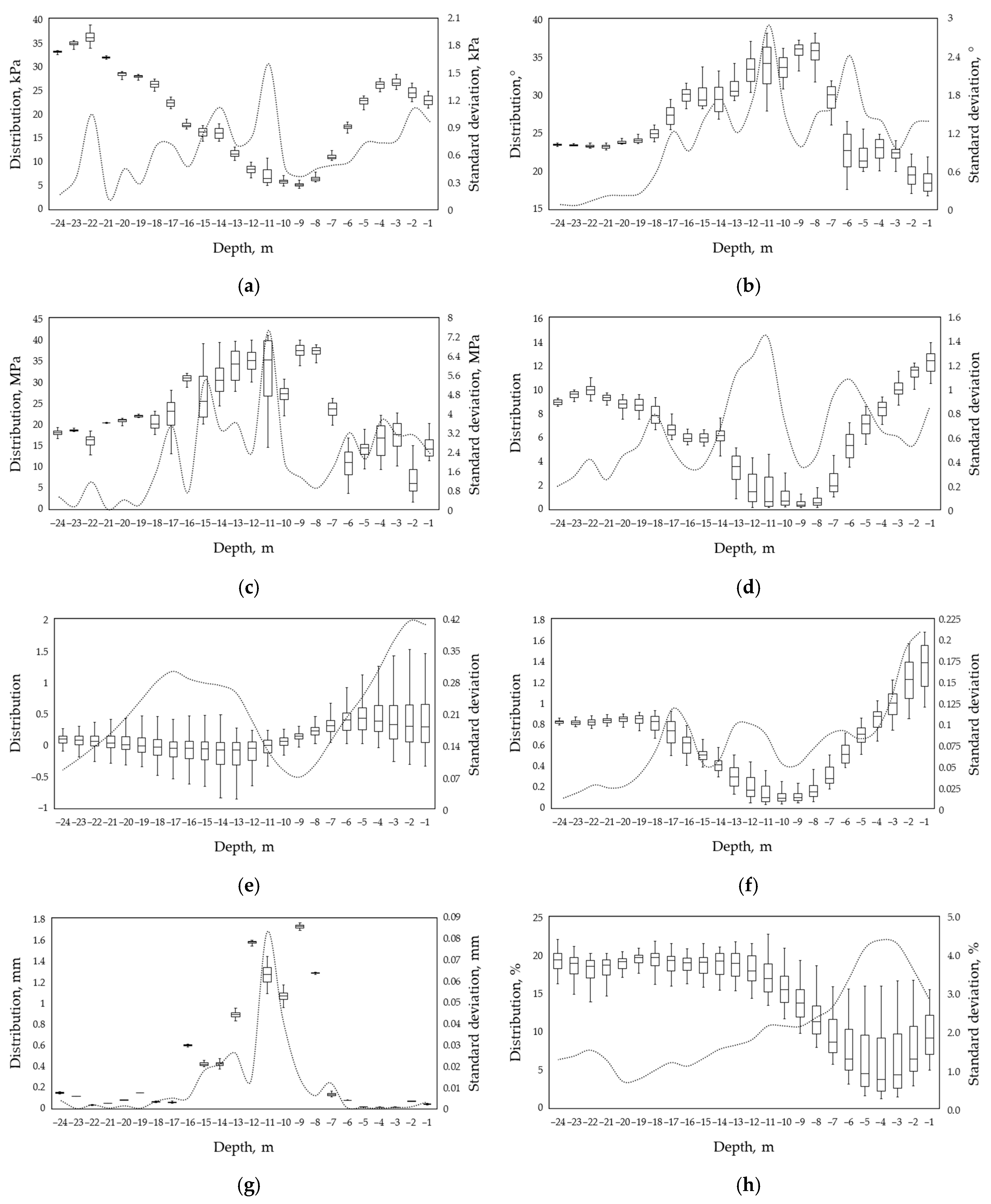
Figure 5 below outlines a more detailed picture of the stratigraphic variation in soil property values by statistically processing and analyzing them using the Box Plot method and calculating the standard deviation for each stratum.

As can be seen from Box Plots in Figure 5, there is a fairly smooth change in the scatter of values of most soil properties with a depth change, except for E and PS—there are sharp jumps in the scatter of values, especially at a depth of 6–12 m for E and 7–16 m for PS. If we consider the scatter of values for each depth separately, it is quite large for all properties except for c and PS. LI, e, and PSD have the highest variation in the upper strata up to a depth of 5 m, while the other properties have the highest variation in the middle strata between 11 and 15 m. The same trend is traced in the standard deviations, where a sharp change in the magnitude of the spread is reflected in the standard deviation curve, creating peaks of different amplitudes. If we look closely at the mean values from the Box Plots, though, we can see that the trend from the color gradients of Figure 4 above is repeated. Here also, φ, E, and PS have high values stretching into the middle strata, c and PSD in the lower strata, and PI and e mostly in the upper strata, and of similar magnitude in the lower strata. Let us consider the interquartile ranges (IQRs) of the values of each property separately. For example, c with a total range of 27.23 kPa (i.e., a difference between 5.9 and 33.13 kPa (Figure 4)) has the highest IQR at 11 m depth and it is about 4 kPa or roughly 15% of the total range. For φ, E, PI, and PS with total sweeps of 14.36°, 24.06 MPa, 9.93, and 1.28, the highest IQR is also observed at 11 m, being about 5° (∼35%), 13 MPa (∼55%), 2.5 (∼25%), and 0.2 (∼16%), respectively. LI, e, and PSD with total spreads of 0.72, 0.87, and 14.91% have the highest IQR observed at 14, 12, and 4 m depths, being about 0.4 (∼56%), 0.2 (∼23%), and 7% (∼47%), respectively. These figures indicate a rather high variability of soil property values at depths from 4 to 14 m, especially for E, LI, and PSD. Based on the example of the site under consideration, it can also be assumed that the values of soil properties by strata can vary between 15 and 56%, or 35.5% on average.

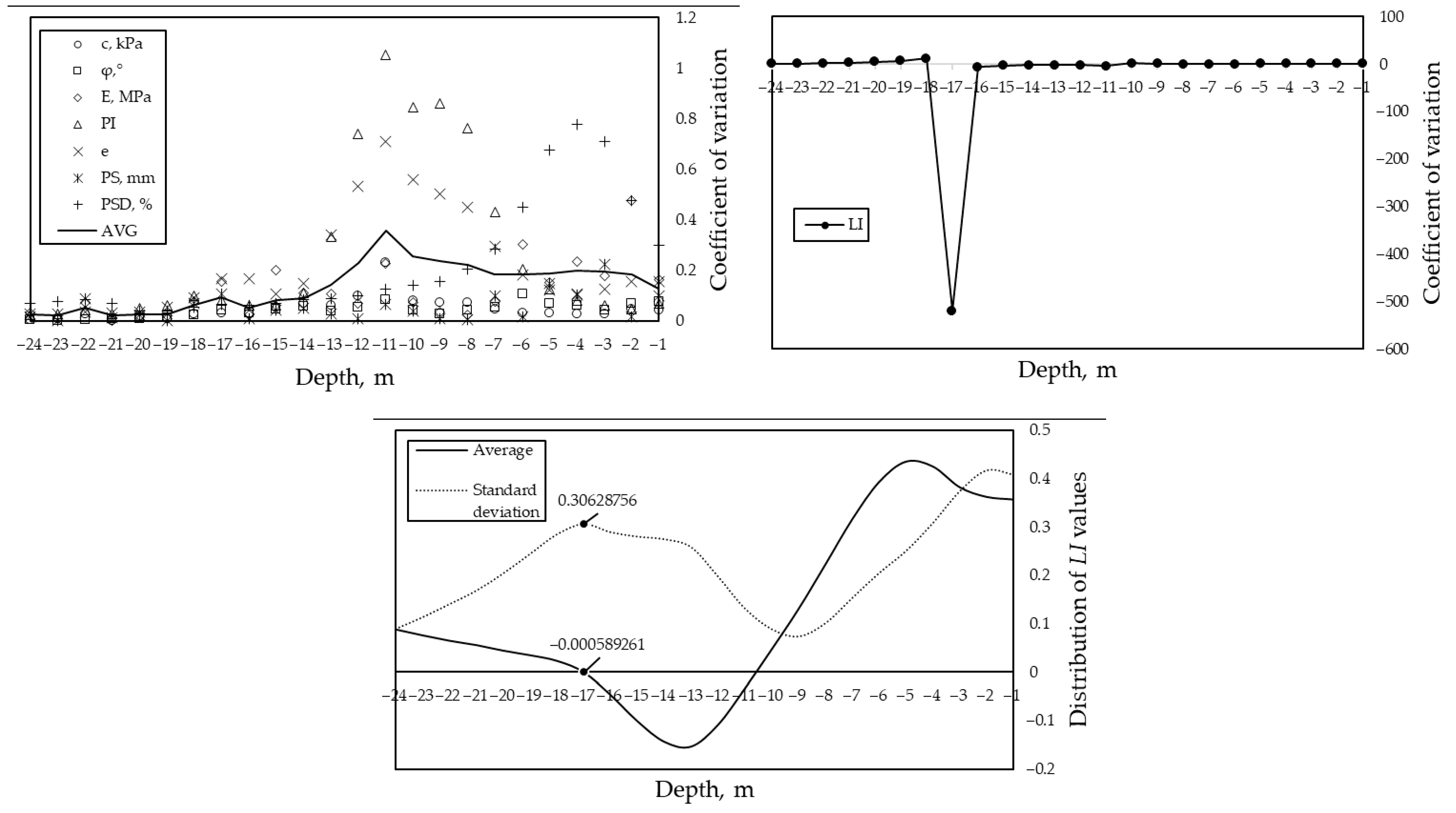
To better analyze the variability of soil property values, coefficients of variation for each depth were calculated (Figure 6).

The scatter plots in Figure 6 show the coefficients of variation of the values of all eight soil properties by depth, which allowed us to compare them with each other on a single dimensionless scale. They are obtained by the ratio of the standard deviations at each depth by their mean values, according to the classical rules of statistics [52]. To improve visual perception, the scatter diagram for LI is separated due to the presence of a deviant value at 17 m depth. In [53], it is explained that the appearance of deviant values of the coefficient of variation is quite probable and acceptable, especially at mean values close to zero, as in our case. As can be seen from the plots, PI, e, PSD, and E have the most variant values, often appearing behind the curve of mean values. LI can also be included in this list if we ignore the deviant value detected. From the scatter of points, it can be seen that at depths from 1 to 13 m, the values are quite variable, with peaks at 11 m depth. From this depth, a decrease in variability is observed.

Table 5. Cross-correlation matrix of soil properties.

Property	c, kPa	φ,°	E, MPa	PI	LI	e	PS, mm	PSD, %
c, kPa		−0.82	−0.69	0.88	0.10	0.79	−0.81	0.08
φ, °	−0.82		0.91	−0.92	−0.38	−0.91	0.86	0.24
E, MPa	−0.69	0.91		−0.77	−0.43	−0.78	0.81	0.35
PI	0.88	−0.92	−0.77		0.21	0.95	−0.82	−0.05
LI	0.10	−0.38	−0.43	0.21		0.35	−0.25	−0.45
e	0.79	−0.91	−0.78	0.95	0.35		−0.78	−0.12
PS, mm	−0.81	0.86	0.81	−0.82	−0.25	−0.78		0.18
PSD, %	0.08	0.24	0.35	−0.05	−0.45	−0.12	0.18

presents the correlation coefficients between all predicted values, reflecting the mutual influence and interdependence of the soil properties of the site under consideration.

The correlation matrix reveals distinct relationships between geotechnical soil properties, with a gradient of blue and red colors representing positivity and negativity of correlations, respectively. A strong positive correlation exists between φ, E, and PS, suggesting that soils with higher shear strength tend to be stiffer and coarser-grained. In contrast, c, PI, and e are also positively correlated among themselves, indicating that fine-grained, cohesive soils are more plastic and porous. Notably, φ is strongly negatively correlated with PI and e, meaning that as soils become more plastic and porous, their frictional resistance decreases. Similarly, E is negatively correlated with PI and e but positively correlated with PS, implying that soil stiffness increases with grain size and decreases with plasticity and porosity. The PI shows a very strong correlation with e (0.95), highlighting that more plastic soils retain more voids. PSD shows weak to moderate correlations with other parameters, indicating that gradation affects soil behavior less directly. The identified dependencies can be used to complement existing practices [1,2,3] in geotechnical surveys.

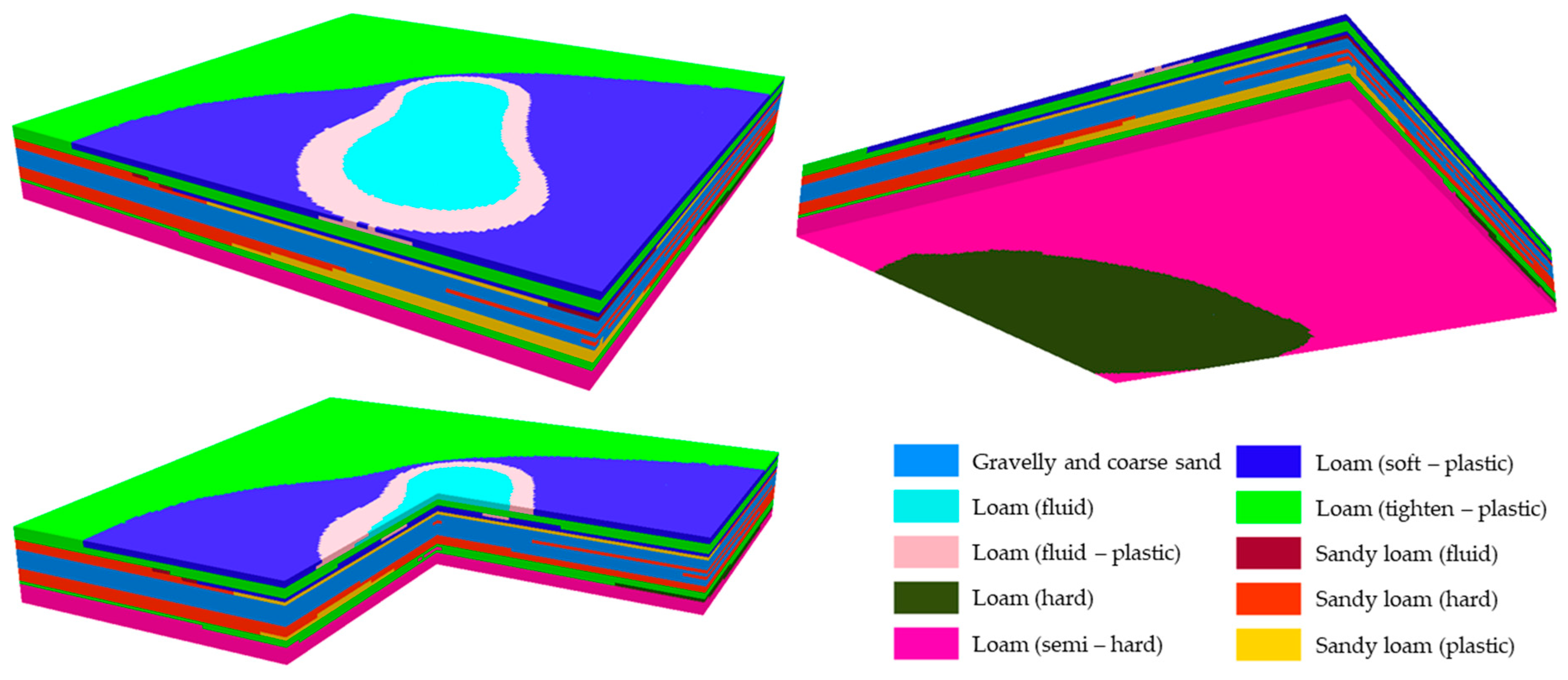
Figure 7 shows the result of soil classification through the tool in Equation (1) represented as a single 3D voxel model.

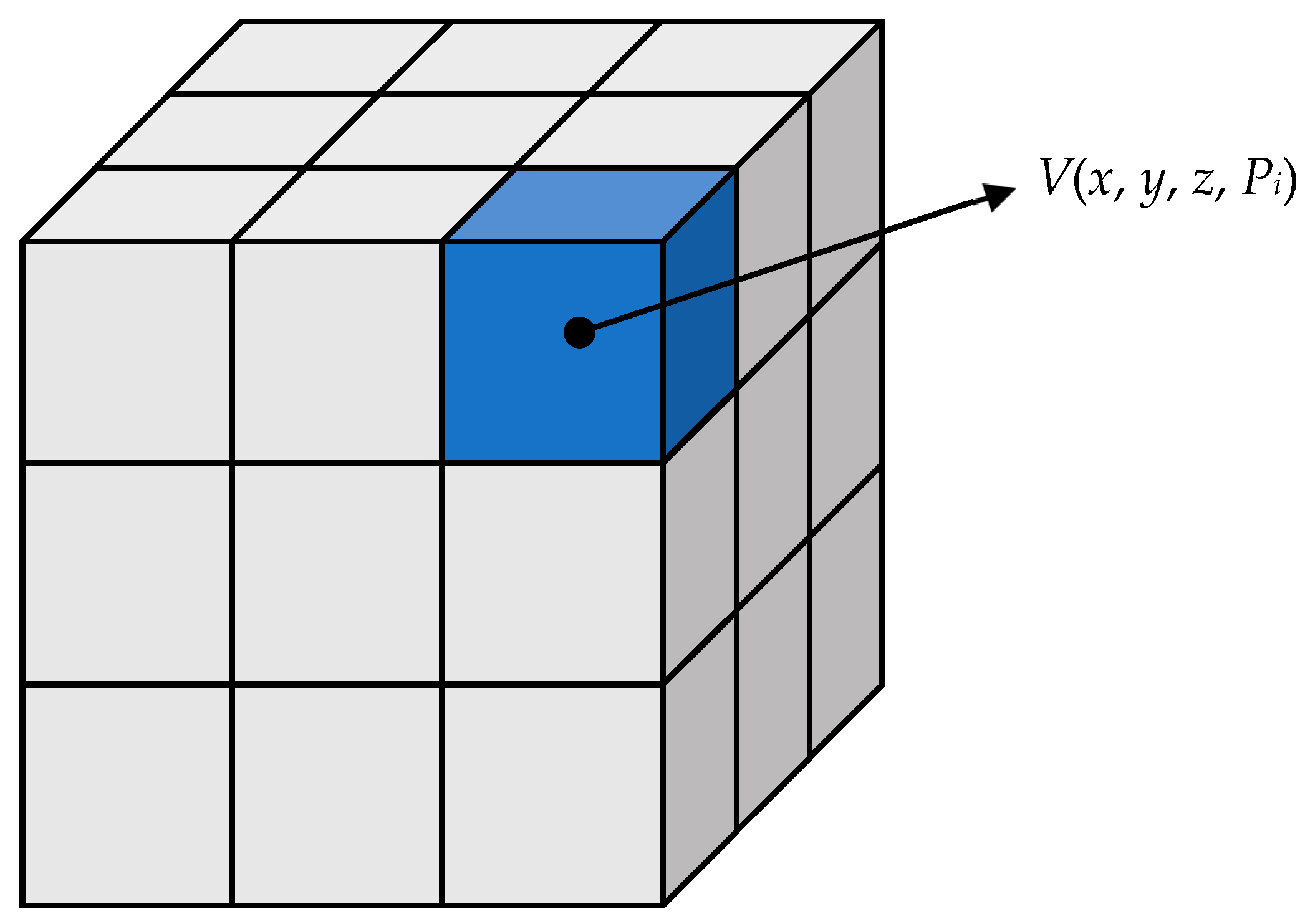
The 3D voxel model from Figure 7 is a digital geometric body of the soil base of the site, discretized into regular volumetric elements—voxels, each of which contains information about the type of soil. The model contains 812,520 voxels (since the dimensions of the soil base are 183 m × 185 m × 24 m). The color differentiation of the voxels indicated in the legend provides visual recognition of the soil type. The model allows us not only to determine the stratigraphic structure of the site, but also to interpret the geotechnical conditions, representing a digital twin of the construction site base. Color transitions between voxels visualize smooth or sharp changes in lithological boundaries, and the presence of clearly traceable boundaries between layers indicates sharp stratigraphic contacts or engineering–geological discontinuities. It is noteworthy that in contrast to the original borehole data, which recorded nine soil types, the classified 3D voxel model displayed ten different types. This indicates the ability of the developed workflow to identify additional lithologic varieties in previously unexplored (hidden) or poorly studied basement zones based on the spatial distribution patterns of geotechnical properties. Thus, the model not only interpolates the known data, but also performs predictive mapping with the possibility of refining the stratigraphic structure. It should be emphasized that the modeling was performed with a resolution of 1 m, i.e., with a voxel size of 1 m × 1 m × 1 m specified in the GA Layer 3D To NetCDF tool, which provided an optimal balance between detail and computational efficiency. Theoretically, reducing the voxel size to centimeter or even millimeter values could lead to more accurate reconstruction of small-scale geological heterogeneities, including interlayers, lenses, and local discontinuities. However, it should be taken into account that increasing the spatial resolution significantly increases the amount of computation and the duration of the workflow operation, from several hours to several days, depending on the performance of the computing platform used to run it. In general, the obtained classified voxel model and best-fit classification function (Equation (1)), which takes into account all input variables (values of eight soil properties in our case), demonstrate greater reliability compared to existing analogs [37,38], which stratify soils only based on interpolation of geometric parameters (i.e., by coordinates) of selected samples, or only one parameter [40,41], avoiding the influence of all others.

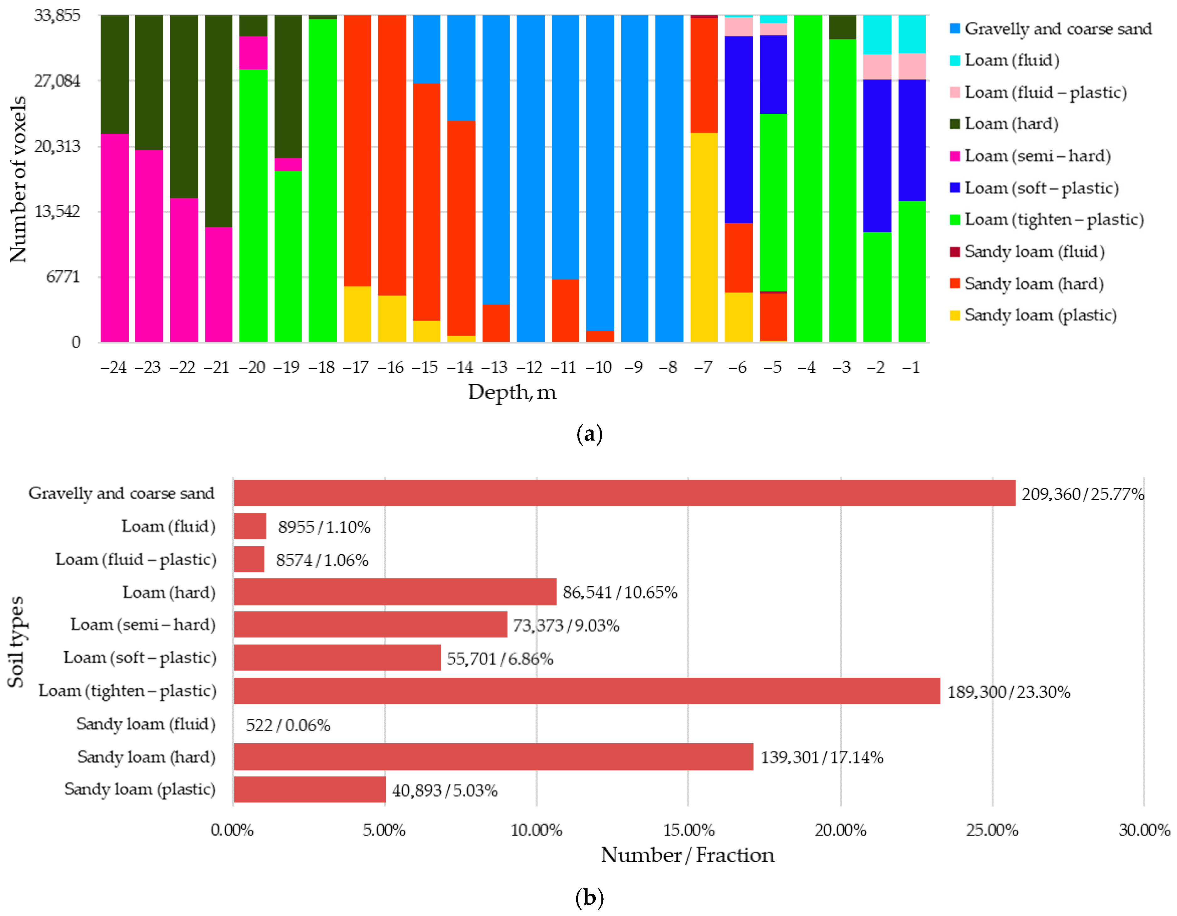
Figure 8 shows the results of the visual–quantitative analysis of the soil types identified in the classified voxel model from Figure 7.

Figure 8 shows the fraction of voxels of each soil type at the base of the construction site, from their total number equal to 812,520. Since the site dimensions in plane are 183 m × 185 m, there are exactly 33,855 voxels at each depth, which can be seen from Figure 8a. The legend of this figure identifies a particular soil type by the color assigned according to the colors assigned in the classified voxel model from Figure 7. Figure 8a shows that loams of various consistencies (fluid, fluid plastic, hard, semi-hard, soft plastic, and tightened plastic) are concentrated mainly in the upper and lower strata at depths between 1 and 6 m and 18 and 24 m, respectively. The sandy loam mainly occupies the middle strata, occurring at depths of 5–7 m and 10, 11, and 13 m, and predominating at 14–17 m depth. Sandy soils occupy most of the middle strata, occurring at depths between 8 and 15 m. Trends of transition and layering of soil strata between each other can also be observed in the figure. Thus, with increasing depth, fluid, plastic, and soft loams are replaced by fluid, plastic, and hard sandy loams. These in turn change to sandy soils, and then back to loams, reflecting the natural layering of soil strata that has occurred historically. It can be observed that there are at least two different soil types per site dimension (i.e., 183 m × 185 m) in all depths except 4, 8, 9, and 12 m, and six different soil types at 5 m depth, reflecting spatial diversity. Figure 8b, in turn, shows the total number of voxels attributable to each soil type along with their percentages. Here, although the number of voxels with sandy soils seems to be the highest, amounting to 209,360 or 25.77%, the total number of voxels belonging to loams still dominates, amounting to 422,444 or 51.99%. Loamy soils account for 180,716 voxels or 22.24%. Very similar fractions were initially identified in the 77 samples from the original well data shown in Table 1 above. Thus, among these samples, about 52% were loams, which is consistent with the voxel–loam fraction of 51.99% from the classified voxel model. The fractions of voxel–sandy loam and –sandy soils are also consistent with slight differences, but with the general trend being maintained, being about 26% for samples and 22.24% for voxels, and 22% for samples and 25.77% for voxels, respectively. These figures indicate a rather high realism of the predicted model and its closeness to natural conditions.

The spatial variability of geotechnical parameters observed in Figure 5, Figure 6, Figure 7 and Figure 8 reflects both the heterogeneity of soil composition and the layered nature of Quaternary deposits in the region. For instance, higher PI and LI values in the shallow depth with lower E and c indicate zones of softer, potentially compressible soils. Conversely, areas with lower PI and LI, coupled with higher φ and E, suggest denser, stiffer soil zones. These patterns may result from historical sedimentation processes and variable groundwater conditions. From an engineering standpoint, such variability directly influences foundation selection. Zones with low stiffness and high plasticity may require reinforced or deep foundations to mitigate settlement risks, while more homogeneous, high-modulus zones may permit cost-efficient shallow foundations. The layered transitions observed in PSD and φ along depth profiles also indicate potential shear interfaces that must be considered in slope stability or retaining wall design. While not the focus of this study, the distributions show expected inverse trends between PI and E, and between LI and φ, reinforcing the geotechnical consistency of the interpolation results.

Table 6. Adjacency matrix of voxel pairs.

No.		Soil Type										Sum	Ratio, %
		1	2	3	4	5	6	7	8	9	10
Soil type	1	581,579	0	0	0	0	0	0	238	62,432	26,031	670,280	28.00
	2		21,312	2071	0	0	0	4953	0	0	166	28,502	1.19
	3			18,603	0	0	2563	4879	0	0	1981	28,026	1.17
	4				219,547	12,478	0	53,617	0	377	0	286,019	11.94
	5					195,505	0	12,900	0	0	0	208,405	8.70
	6						126,838	41,867	266	4630	17,599	191,200	7.98
	7							477,755	328	34,662	8211	520,956	21.75
	8								920	349	50	1319	0.06
	9									361,860	5786	367,646	15.35
	10										92,520	92,520	3.86
Total:												2,394,873	100.00

presents the results of the analysis of soil stratification patterns in the form of an adjacency matrix containing the number of pairs of neighboring voxels represented by the 10 soil types found in the classified voxel model: (1) gravelly and coarse sand; (2) loam (fluid); (3) loam (fluid plastic); (4) loam (hard); (5) loam (semi hard); (6) loam (soft plastic); (7) loam (tightened plastic); (8) sandy loam (fluid); (9) sandy loam (hard); (10) sandy loam (plastic).

Table 6 is a symmetrized matrix representing the number of unique pairs of adjacent voxels within the base of the site. In this matrix, the diagonal values correspond to internal homogeneity—the number of pairs of neighboring voxels of the same soil type—while the non-diagonal elements indicate the contact zone between different soils. Visually, diagonal values are colored in a blue color gradient, while transitions between different types are colored in a red color gradient, allowing an intuitive assessment of the degree of internal connectivity and lithologic transitivity. Gravelly and coarse sand make the maximum contribution to the total number of neighboring pairs—28%, showing both significant homogeneity and high density of juxtaposition with other types, primarily sandy loam (hard) (62,432 pairs) and sandy loam (plastic) (26,031 pairs). This may indicate a thick channel or alluvial horizon where coarse clastic material forms the base of the stratigraphic sequence. Loam (tightened plastic) (21.75%), characterized by high internal cohesion (477,755 homogeneous pairs) as well as active contacts with loam (soft plastic) (41,867), loam (hard) (53,617), and sandy loam (hard) (34,662), is the second largest contributor. These transitions indicate a complex facies structure associated with varying moisture, density, and depositional conditions within the loamy horizon. Loam (hard) (11.94%) and loam (semi-hard) (8.70%) also exhibit marked homogeneity and a tendency toward mutual neighborhood, supporting the assumption of a stratigraphic sequence of layer formation with a gradual decrease in density and plasticity. Less-represented but lithologically significant types are also of interest: sandy loam (hard) (15.35%) and sandy loam (plastic) (3.86%), showing a clear contact boundary with coarse clastic and loamy material. This may reflect conditions of seasonal changes in water saturation or hydrodynamic stratification. Thus, the matrix allows not only to quantify the degree of heterogeneity of the base, but also to identify the probable directions of transitions between lithotypes, which is absent in existing solutions [28,29,37,38,40,41], and is important information for qualitative modeling of engineering–geological conditions, definition of facies boundaries, and justification of design solutions in construction.

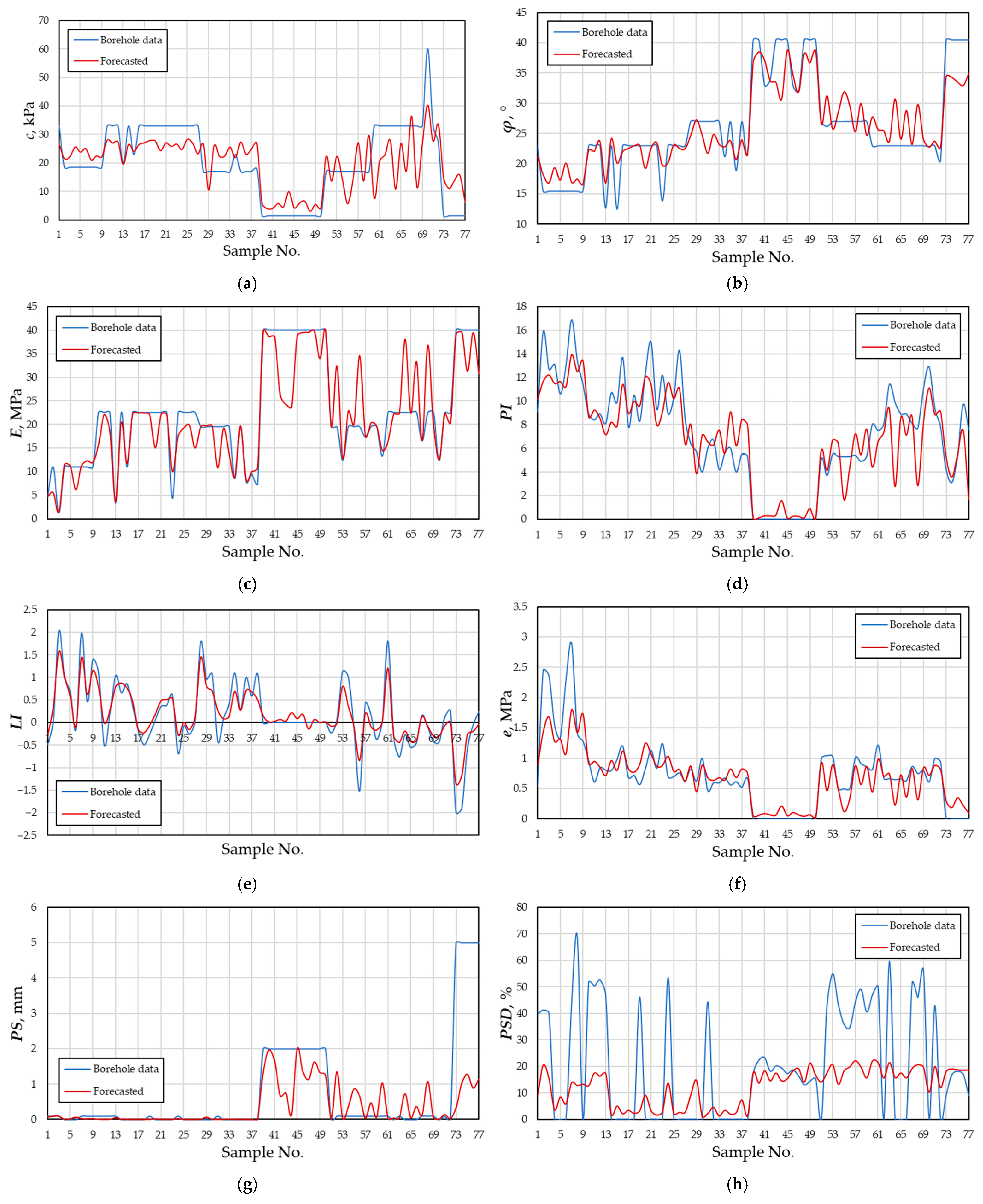
In order to evaluate the reliability of the developed workflow and validate it, Figure 9 shows the results of a comparative analysis between the values of soil properties from 77 borehole samples (Table 1) and the values predicted by the workflow in the same coordinates extracted from voxel models (Figure 4).

Figure 9 shows through curves of two colors (blue and red) the values of eight soil properties (c, φ, E, PI, LI, e, PS, and PSD) obtained by testing 77 borehole samples and the predicted values at the same points in the footprint of the site, respectively. As can be seen from the figure, fairly consistent trends between the curves of the borehole data and the predicted values for most of the soil properties are tracked, which confirms the performance of the proposed workflow. 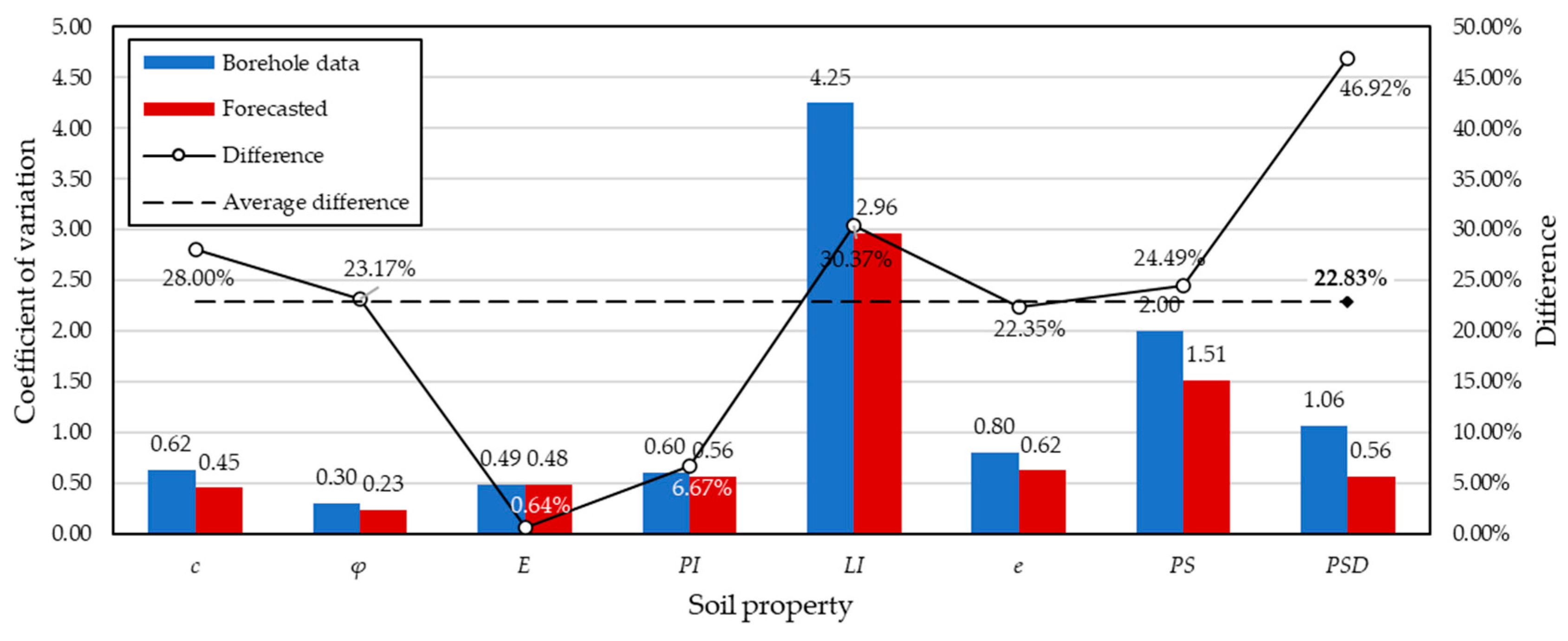The most uncoordinated were the PSD values. Despite this, we can see from the curves that the predicted values even look somewhat smoothed, as if recognizing anomalies of borehole data and smoothing them out, obeying the natural distribution and excluding the human factor when classifying soils during the preparation of the engineering–geological survey report. To verify this smoothing tendency, coefficients of variation (CV) for each soil property were calculated for the borehole and predicted data (Figure 10) from their values for 77 samples (for borehole data) and points (predicted at the same locations). The smoothing hypothesis in this case was that the coefficients of variation of the predicted values should turn out to be somewhat smaller than those of the borehole values.

Figure 10 above shows that for all soil properties, the predicted values of the CV were smaller than those of the borehole data, thus confirming the above hypothesis. Thus, the original borehole data have CV between 0.3 and 4.25, while the predicted data have CV between 0.23 and 2.96, with mean values of 1.27 and 0.92, respectively. It is noticeable that most of the values of the CV do not exceed one. However, there are deviant ones, for example, in the case of LI and PS, many times higher than the other values. This can speak either to the actual variety of values obtained within the geotechnical engineering survey, or to some kind of error in their execution (i.e., human factor), suggesting the need for careful statistical processing of data when performing geotechnical surveys, as in our case. The difference between the CV in percentage terms is between ∼0.64% (for E) and ∼46.92% (for PSD), averaging 22.83%. According to this indicator, we can assume that the approximate degree of accuracy of the proposed workflow is more than 77%, which is quite a bit higher than, for example, that of [29], who achieved an accuracy of 60% when interpolating the available water content.

To rigorously validate the accuracy of the proposed geoprocessing workflow, a paired t-test was conducted comparing interpolated values with the borehole measurements for eight geotechnical properties (

Table 7. T-test and CI results.

Property	Mean Difference	95% CI Lower	95% CI Upper	p-Value	Significant (p < 0.05)
c [kPa]	−0.506395185	−2.444450206	1.431659836	0.604294134	No
φ [°]	−0.0359116	−0.842874278	0.771051079	0.92960611	No
E [MPa]	−0.84016846	−2.093179855	0.412842935	0.185713394	No
PI [%]	−0.412187799	−0.888180936	0.063805338	0.088647324	No
LI	0.004218829	−0.059715301	0.06815296	0.895786608	No
e	−0.042087884	−0.112119242	0.027943475	0.235039462	No
PS [mm]	−0.306118697	−0.554443651	−0.057793743	0.016366152	Yes
PSD [%]	−7.86300294	−12.02530505	−3.700700834	0.000328995	Yes

). Additionally, 95% confidence intervals (CI) for the mean differences were calculated (Table 7).

The t-test results indicated no statistically significant differences (at α = 0.05) between predicted and observed values for six out of eight soil properties, including c, φ, E, PI, LI, and e (p > 0.05). This supports the conclusion that the interpolated values generally match the borehole data with minor, statistically insignificant discrepancies. However, statistically significant differences were observed for the PS and PSD (p = 0.0164 and p = 0.00033, respectively). These deviations are attributed to the inherent smoothing effect of spatial interpolation, particularly for highly localized or discontinuous variables like PSD. This effect is further visible in Figure 9, where PSD appears smoothed relative to borehole spikes. CV comparisons in Figure 10 also reflect this behavior. The CV values for predicted PSD were lower than those from borehole data, confirming reduced variance due to interpolation. Yet this smoothing does not invalidate the workflow; instead, it reflects the trade-off between spatial continuity and high-frequency local detail. While direct validation was performed using borehole vs. predicted values, future work will involve additional cross-validation or evaluation against independent datasets to further assess generalizability.

4. Conclusions

A voxel-based geoprocessing workflow using EBK 3D and a best-fit convergence function was successfully developed and implemented to model eight geotechnical properties (cohesion (c), friction angle (φ), deformation modulus (E), plasticity index (PI), liquidity index (LI), porosity (e), particle size (PS), and particle size distribution (PSD)) in 3D across a 183 m × 185 m × 24 m site in Astana, with a resolution of 1 m × 1 m × 1 m.

The resulting voxel model, containing over 812,000 elements, accurately captured the stratified and heterogeneous nature of the subsurface, revealing depth-dependent variations in cohesion, friction angle, deformation modulus, and plasticity indices.

Soil classification using a multivariate discrepancy-based function identified 10 soil types, including one not recorded in borehole data, confirming the model’s ability to detect hidden lithological zones and improve geotechnical zoning.

The predicted proportions of soil types closely matched the initial borehole distribution (e.g., loams: 51.99% vs. 52%), validating the model’s representativeness of natural conditions.

Adjacency analysis of 2.39 million voxel pairs revealed significant internal homogeneity and transition trends, particularly in gravel–sandy and stiff loam zones, supporting realistic stratigraphic modeling.

The workflow showed strong consistency with borehole data, with no significant differences detected for six out of eight geotechnical properties (p > 0.05), confirming statistical reliability. Minor deviations in PS and PSD were attributed to expected smoothing effects of spatial interpolation and did not compromise the overall accuracy of the model.

Limitations and Future Scope

This study was limited to eight core geotechnical properties and used a fixed voxel resolution of 1 m. Higher-resolution modeling (e.g., millimeter scale) and inclusion of hydro-physical or chemical parameters may yield more detailed insights but require significantly more computational resources. Additionally, while validation was performed using the same dataset, independent cross-site validation is needed for broader generalizability.

Future work should explore integrating groundwater conditions, seasonal variability, and structural response modeling into the voxel-based workflow. The classification function can also be adapted to other soil standards, enabling widespread use in automated digital ground modeling and infrastructure design optimization.