1. Introduction
Optimizing energy use and managing thermal conditions in industrial buildings are critical challenges in the context of the energy transition and reducing greenhouse gas emissions. Efficient management of Heating, Ventilation and Air-Conditioning (HVAC) systems is essential to ensure occupant comfort, maintain optimal production conditions, and minimize energy consumption [
1,
2]. In this context, Artificial Intelligence (AI) is emerging as a solution for predicting and controlling indoor temperatures.
In response, recent French regulations promote infrastructure modernization to address energy efficiency goals. The French Law ‘Évolution du Logement, de l’Aménagement
et du Numérique (ELAN)’ sets ambitious targets for the energy performance of buildings, notably through the integration of intelligent thermal management technologies [
3]. The tertiary sector decree requires buildings for tertiary use to progressively reduce their final energy, thus necessitating advanced control solutions and predictive systems for greater energy efficiency [
4]. In addition, the Building Automation and Control Systems (BACS) decree requires the installation of building automation and control, reinforcing the interest in predictive models capable of optimizing thermal conditions in real time and anticipating temperature variations [
5].
Thermal comfort is a central issue in the design and management of intelligent buildings, particularly in a context where energy sustainability and occupant wellbeing have become major priorities. Standards such as ISO 7730 [
6] and ASHRAE 55 [
7] play a fundamental role in providing methodological frameworks for assessing and guaranteeing a comfortable thermal environment. These standards are grounded in models that incorporate environmental and physiological parameters, such as Predicted Mean Vote (PMV) and Predicted Percentage of Dissatisfied (PPD) for ISO 7730, and adaptive approaches for ASHRAE 55 [
8,
9].
Historically, thermal prediction models have relied on physical and statistical approaches. Although robust, these methods have limitations when faced with the dynamic and complex environments of industrial buildings, notably due to their inability to capture the non-linear interactions and temporal dependencies of environmental parameters [
10]. As traditional models reached their limits, new approaches emerged: Machine Learning (ML) and Deep Learning (DL) techniques have enhanced the accuracy and flexibility of predictive models, opening up new perspectives for energy optimization and intelligent thermal control [
11].
This study proposes to analyze and compare seven AI-based approaches (including three ML approaches and four DL approaches) to predict temperature in an industrial building. This comparative study focuses on AI algorithm performance rather than comparison with physical models, whose limitations are well established in existing literature. Using a dataset from an industrial workshop equipped with environmental sensors, the performance of 7 predictive models is evaluated, with a focus on their accuracy and ability to adapt to dynamic environments.
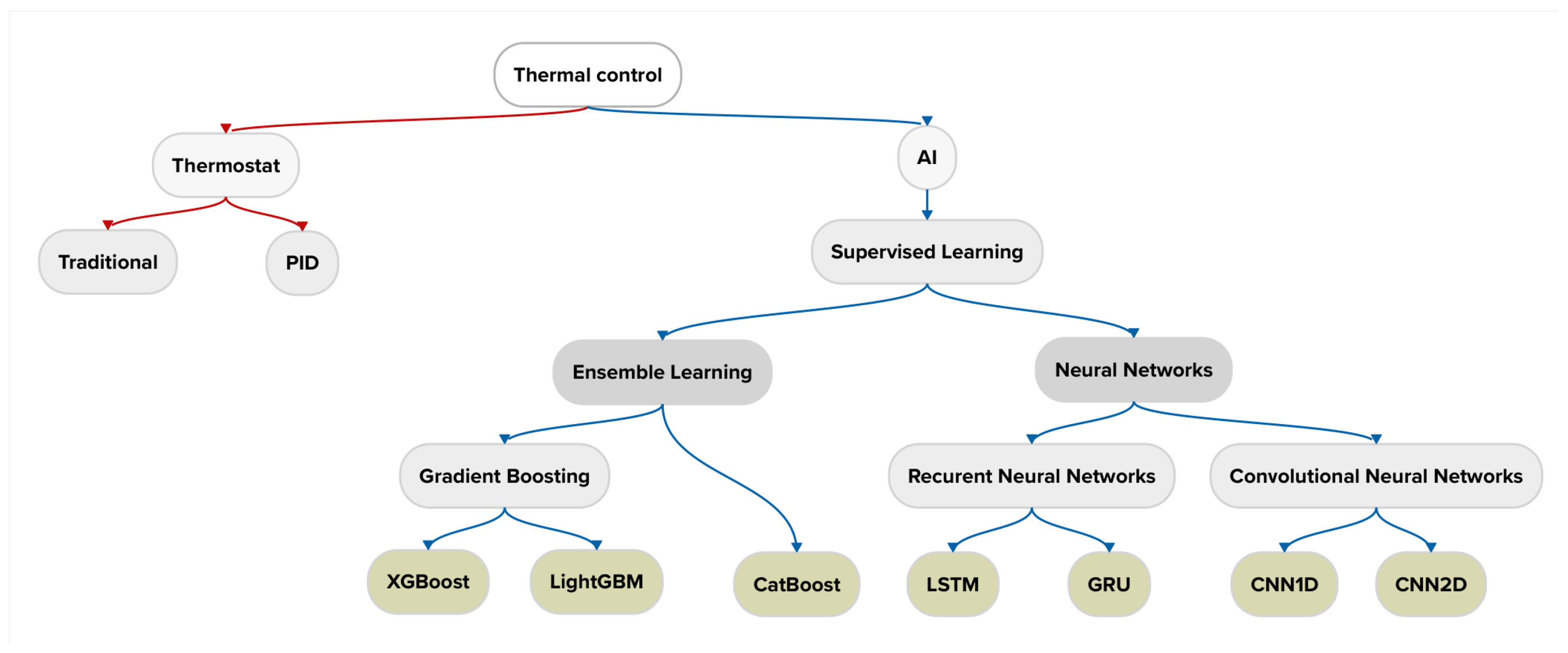
The various artificial intelligence approaches utilized in this study can be categorized into distinct algorithmic families, as illustrated in
Figure 1. This mind map provides a comprehensive overview of the machine learning and deep learning techniques relevant to temperature prediction tasks. The left branch represents traditional machine learning algorithms, including the Gradient Boosting methods (XGBoost, LightGBM, and CatBoost) employed in our comparative analysis. The right branch displays deep learning architectures, highlighting the neural network models (LSTM, GRU, CNN1D, and CNN2D) that we evaluate for their predictive capabilities in industrial environments.
This research evaluates and compares the performance of seven AI-based approaches for temperature prediction in an industrial workshop, including XGBoost, LightGBM, and CatBoost (ML), as well as LSTM, GRU, CNN1D, and CNN2D (DL). The objective is to identify the most suitable model by balancing predictive accuracy, computational efficiency, and robustness to varying industrial conditions, with the goal of maximizing energy efficiency and enhancing thermal comfort. This work contributes to the broader movement of technological innovation in the context of Industry 4.0, promoting intelligent management of industrial buildings through advances in AI and DL while adhering to current legal requirements.
4. Data Preparation and Processing
4.1. Database Data Collection and Analysis
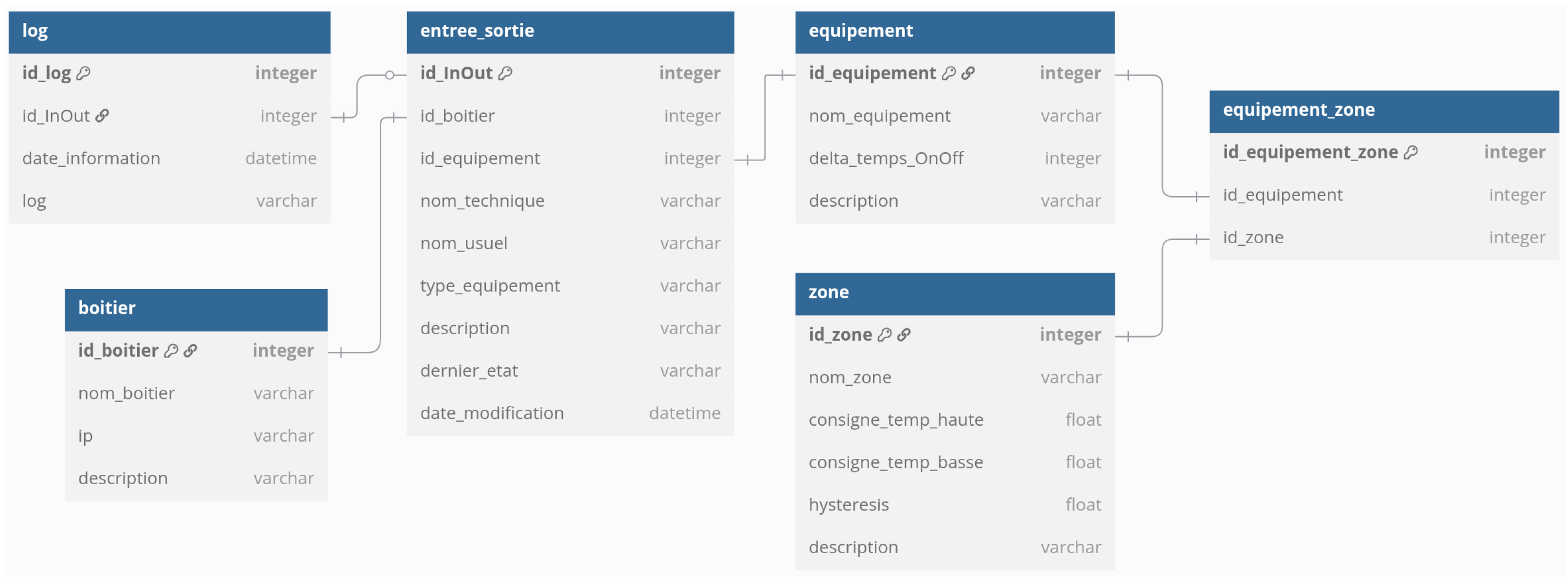
Workshop data is stored in a MySQL/MariaDB relational database. The system’s architecture enables the control units to manage several pieces of equipment simultaneously, each input/output being dedicated to the control of a specific element of the equipment.
Figure 3 illustrates the structure of this database, revealing an organization centered on operational needs rather than AI modeling requirements. This architecture, designed for daily facility management, required significant transformation to be usable by our predictive algorithms.
An extraction of this database was performed on 17 April 2024 at 10:20, comprising 42,222,594 rows and 3 columns covering the period from 12 October 2022 at 17:09:35 to 17 April 2024 at 10:20:45. This considerable volume of raw data underwent comprehensive processing including cleaning, normalization, and extraction of relevant features for machine learning.
Following this preparation process, a structured dataset was constructed of 124,700 rows and 100 columns. This transformation allowed the isolation of essential predictive variables while preserving the integrity of temporal and causal relationships necessary for modeling the building’s thermal behavior. Only a subset of these data proved relevant for training the predictive models, with the other variables primarily serving for contextualization and results validation. The feature set focuses on temporal lags and direct system states (relay positions, door states) rather than complex derived features, which is consistent with the building’s low thermal inertia characteristics, where instantaneous relationships dominate over complex temporal patterns.
4.2. Data Transformation Methodology for Modeling
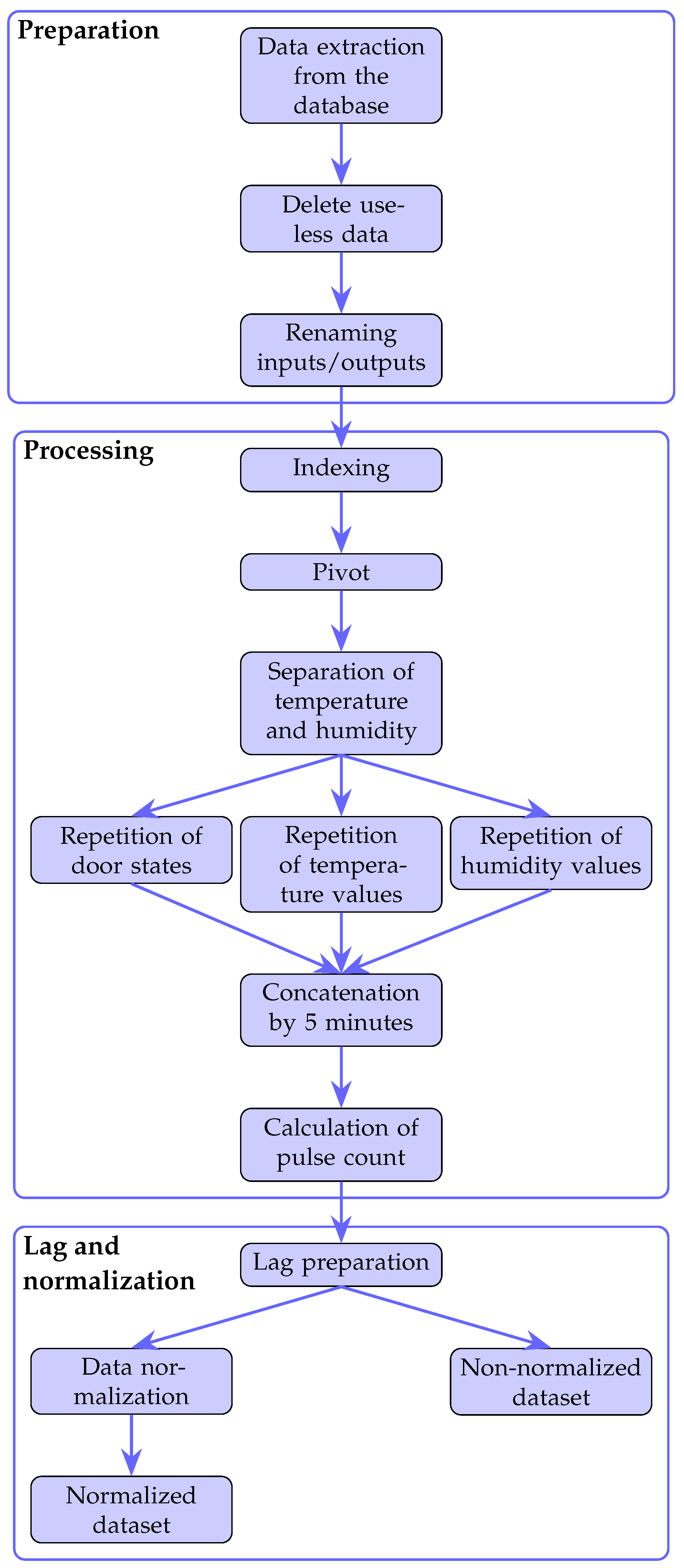
The data transformation methodology is built around a set of essential steps [
30]. The complete process, illustrated in
Figure 4, is organized into three main phases:
Preparation
Processing
Lag and normalization
4.2.1. Preparation Phase
This phase includes the initial steps to structure and clarify the dataset:
Data extraction: Raw data is extracted from the database in CSV format, retaining only relevant information.
Table 1 and
Table 2 illustrates the structure of this dataset, moving from an initial format
Table 1 to a transformed format
Table 2.
Delete useless data: Lighting control information (including “passageway lighting” and “outdoor lighting”) has been removed from the dataset, as it is not relevant to the analysis. System monitoring elements such as “heartbeat” and “Arduino Heartbeat” signals have also been excluded, since they do not provide meaningful information for this study.
I/O renaming: Technical identifiers are replaced by explicit names to facilitate analysis (e.g., tempEXT, HumExt, PP4).
4.2.2. Processing Phase
This phase covers transformation and feature engineering operations required for modeling:
Indexing: Each record is indexed by date and time to allow chronological sorting and time-based data analysis.
Pivot: The dataset is reorganized with variables as columns and timestamps as rows, improving its suitability for analysis.
Temperature and humidity separation: These variables are split into distinct series to allow independent analysis of their influence.
State repetition: Values for door states, humidity, and temperature are repeated to create continuous time series. Temperature and humidity are interpolated, while door state data is filled using the forward fill (ffill) technique.
Concatenation by 5 min: Data is grouped into 5 min intervals, forming regular time series as shown in
Table 2. This interval balances the need for meaningful resolution and reduced sensitivity to noise, particularly given the high thermal inertia of the building.
Pulse count calculation: The number of gas pulses is computed for each interval, providing a quantifiable measure of gas consumption.
4.2.3. Lag and Normalization Phase
This final phase prepares the dataset for input into modeling algorithms:
Lags preparation: Time-shifted variables are created to represent the system’s past states. This consists of associating variable values from previous intervals with the current time step.
Data normalization: Features are normalized to reduce scale-related bias and enhance model convergence, particularly for algorithms sensitive to input magnitudes.
This process results in two versions of the dataset: a normalized dataset and a non-normalized one. The choice between them depends on the model used: neural networks typically require normalized inputs using MinMax scaling to facilitate convergence, whereas other models can operate directly on raw data.
4.3. Selection of Relevant Data for Analysis
The building under study is heated from October to April. Consequently, the analysis of temperature data focuses on this heating period, when thermal variations are significant and relevant to the study. During summer months, heating is unnecessary as external temperatures consistently exceed comfort thresholds, making this period irrelevant for evaluating heating system performance and control algorithms.
To guarantee the reliability of results, the selected period for data processing runs from January 25 to 3 April 2024. This period was chosen because it corresponds to the timeframe during which all sensors functioned perfectly, thus ensuring data collection without any gaps or major anomalies. This January–April period also encompasses significant seasonal variation, with external temperatures ranging from negative values in winter to approximately 20 °C in early spring, providing robust evaluation conditions for model generalization across changing climatic conditions. Earlier attempts at data collection were compromised by significant issues with the gas consumption sensors, which produced intermittent readings and occasionally reported physically impossible values. Additionally, the building management system experienced several software failures during the fall months, resulting in corrupted data logs and unreliable control signal records.
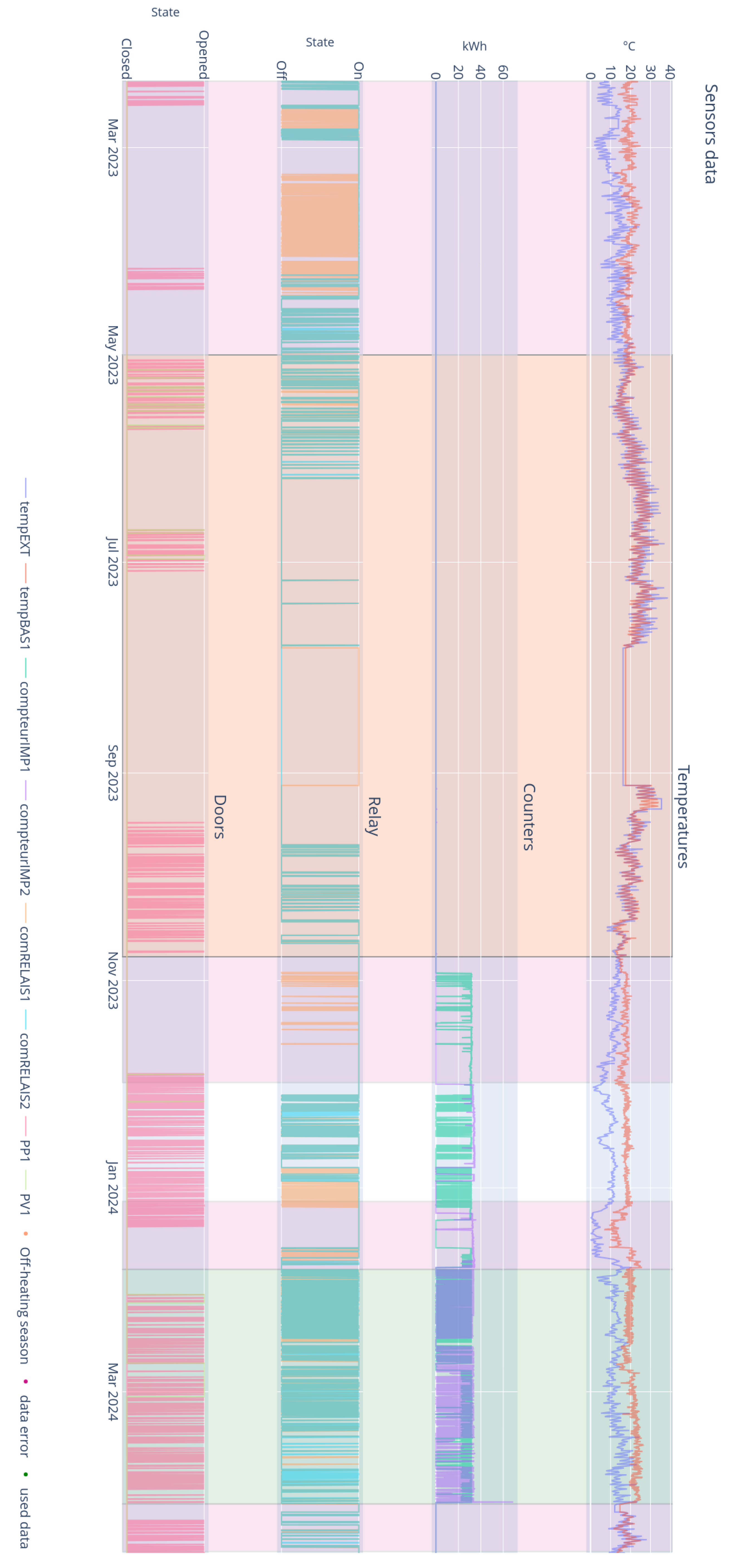
Figure 5 presents a comprehensive visualization of the prepared data spanning fifteen months, enabling assessment of their distribution and quality before implementation in predictive models. This visualization is structured in four distinct panels illustrating: internal (tempBAS1) and external (tempEXT) temperature variations, energy consumption readings in kWh, operational states of the heating system control relays, and building door activity. Seasonal cycles are clearly observable, with external temperatures fluctuating between negative values in winter and reaching approximately 30 °C in summer, while internal temperature is maintained around 15–20 °C during the heating season. The colored background sections indicate different operational periods, including off-heating seasons, data error instances, and the data segments effectively used for analysis.
Only the selected period from January to April provides suitable conditions for AI model testing, as it represents the only timeframe when the entire monitoring and control infrastructure was fully operational, with all sensors reporting accurate readings and the control system responding as designed.
5. Design and Evaluation of Prediction Models
5.1. Hypotheses and Experimental Design
Modeling focused on a specific temperature sensor: This strategy consists in developing a predictive model dedicated to the temperature of a single sensor, rather than seeking to simultaneously predict the temperatures of all the sensors on the shop floor. The temporal validation strategy employed a chronological split to evaluate model performance on unseen seasonal data, avoiding the data leakage issues inherent in traditional cross-validation approaches for time series. This decision is based on the principle of parsimony, aimed at building a robust and interpretable initial model, in line with the recommendations in the time series modeling literature [
31].
Determining the optimum prediction horizon: The prediction horizon, defined as the time interval over which forecasts are made, is a crucial parameter for the practical application of the model. Too short a horizon limits the usefulness of forecasts for decision-making, while too long a horizon can lead to a degradation in accuracy. In this study, prediction horizons of 1, 12, and 24 time steps are tested, corresponding to 5 min, 1 h, and 2 h, respectively. A preliminary investigation into the thermal response characteristics of the building revealed that heating control equipment typically begins to produce measurable effects within 5 to 10 min after activation. This timescale is well suited to the computational capabilities of standard industrial hardware, where model inference times of milliseconds are easily achievable within 5 min control cycles. Reaches the target temperature in 1 h on average, with the slowest systems taking just under 2 h to fully respond. This finding indicates that a 2 h prediction horizon is sufficient for effective operational decision-making, as it encompasses the full response cycle of the heating systems while maintaining prediction accuracy within acceptable parameters.
Selecting the right number of lags: The number of lags, or past temperature values included as input variables, determines the model’s ability to capture time dependencies. An insufficient number of lags can lead to under-modeling. on the opposite, an excessive number can introduce noise and increase the risk of overlearning (overfitting) [
32]. During the preliminary investigation mentioned previously, a low significance of the lag effects was observed in this particular building’s thermal behavior. The elbow method applied indicated an inflection point between 1 and 5 lags, depending on the algorithms used. Feature selection experiments confirmed that the selected variables effectively captured the essential predictive relationships without requiring complex derived features. However, for neural network models specifically, a lag parameter of 5 was determined to be sufficient to capture any relevant temporal dependencies while maintaining model efficiency and preventing overfitting issues. This conservative choice was made to ensure parameter count compatibility with the available dataset size (124,700 rows post-transformation).
5.2. AI Models Used for Prediction
For temperature prediction, several families of algorithms were compared.
Figure 1 provides a mind map illustrating the different families of algorithms used in this study:
XGBoost and LightGBM: Tree-based Gradient Boosting methods. These approaches handle tabular data well and offer robust performance for many regression problems. Additionally, these models provide inherent interpretability through feature importance rankings, enabling identification of the most influential variables for industrial decision-making.
CatBoost: A Gradient Boosting variant adapted to categorical variables, direct use of relay positions, and other discrete sensors in nominal form.
LSTM and GRU: Two recurrent neural network architectures specifically designed for sequence modeling and time series analysis. LSTMs incorporate input, output, and forget gates to control information flow through the network and address the vanishing gradient problem. GRUs use a simpler architecture with reset and update gates, requiring fewer parameters than LSTM while still effectively capturing long-term dependencies.
CNN1D and CNN2D: Convolutional network approaches. CNN1D considers the time vector as a one-dimensional sequence. The CNN2D, on the other hand, treats the lags and the various variables as an “image” (height = number of lags, width = number of sensors/features), enabling spatio-temporal motifs to be captured across all sensors. The neural network architectures were designed with controlled parameter counts to ensure compatibility with the dataset size. Specifically, the CNN2D model was limited to fewer than 50,000 trainable parameters through constrained filter numbers and fully connected layer sizes. All deep learning models incorporated regularization techniques: dropout layers (rates 0.2–0.5) for CNN architectures and L2 regularization for recurrent models to prevent overfitting.
For neural networks, a training protocol including early stopping on a validation set was used to limit overlearning. Gradient Boosting approaches (XGBoost, LightGBM, CatBoost) were trained on the training part, then validated on the test part.
5.3. Preparation of Lagged Variables
Data was collected and prepared to test the different algorithms. The data came from a workshop equipped with temperature, humidity and heating control sensors (knob positions, relays, gas meter). Measurements were collected chronologically, then assembled into a set of features, including outdoor temperature and humidity.
To enable models to exploit time dependency, delayed features (lags) were created. For each variable (e.g., temperature), the corresponding lagged values were generated, where n corresponds to the number of lags (past values). The objective is to predict, at time t, the value of the temperature at a horizon (where in our experiments). All existing columns (temp, humidity, relay positions, etc.) were thus shifted in time, and a dataset with these lagged variables was constructed for training. The first few rows, lacking complete past values, were eliminated so as not to introduce any missing values. Preliminary tests with feature reduction techniques showed no significant performance improvement, indicating that the transformed dataset was appropriately dimensioned for the algorithms evaluated.
The dataset was then split into a
training part (80% of observations) and a
test part (20%), respecting the temporal order to ensure realistic evaluation of model performance on unseen future data, including seasonal transitions from winter to spring conditions. In some cases (XGBoost, LightGBM, LSTM, etc.), normalization or
scaling (MinMax, for example) was applied to facilitate model convergence. For CatBoost, on the other hand, categorical columns (buttons, relays) were kept as is, as CatBoost is capable of handling categorical variables natively [
21].
5.4. Hyperparameter Tuning Strategy
In this study, the primary objective consists of conducting a comparative analysis across a wide spectrum of machine learning and deep learning models under realistic deployment constraints. Therefore, a pragmatic and consistent tuning strategy was employed that balanced methodological rigor with computational feasibility across all seven models [
33,
34].
For the machine learning models (XGBoost, LightGBM, CatBoost), manual tuning informed by domain knowledge was employed, complemented by limited grid search over key hyperparameters. Following established best practices [
35,
36], the tuning focused on the following:
Learning rate (0.01 to 0.1);
Maximum tree depth (3 to 8);
Number of estimators (100 to 1000);
Subsampling ratios (0.7 to 1.0).
These parameter ranges were selected based on prior literature recommendations [
35,
37] and internal validation performance. The tuning protocol aimed to avoid overfitting while preserving computational efficiency, particularly given the recursive prediction scheme and multi-horizon evaluations.
For the deep learning models (LSTM, GRU, CNN1D, CNN2D), a constrained architecture search space was defined to maintain computational tractability [
38,
39]. Within this space, the following parameters were tuned:
Number of recurrent units or filters (32 to 128);
Dropout rate (0.2 to 0.5) [
40];
Number of layers (1 to 2);
Batch size and learning rate (32 to 128 and 0.001 to 0.01, respectively).
Early stopping on validation loss was employed to determine optimal training epochs, with a patience parameter of 10 epochs and a minimum improvement threshold of 0.001 [
39,
41]. This approach prevented overfitting while ensuring adequate model convergence across all neural network architectures.
This approach prioritizes consistent methodology across model families rather than exhaustive optimization of individual models, reflecting the trade-offs industrial practitioners face when selecting and deploying predictive algorithms [
37]. This strategy helps prevent selection bias that can arise when models receive unequal optimization effort [
42], ensuring fair comparison across different algorithmic approaches.
While more sophisticated optimization methods such as Bayesian optimization could potentially enhance individual model performance [
34], the chosen approach allowed for meaningful comparison across model families without introducing selection bias or overfitting to validation data, reflecting realistic constraints faced in industrial deployments.
5.5. Recursive Multi-Step Forecasting Strategy
To ensure data leakage prevention and reflect real-world deployment conditions, this study employs a recursive multi-step prediction approach, which is particularly well suited for real-time applications in industrial control. In this paradigm, the model is trained to predict the target variable (indoor temperature) at the next time step, denoted as , based on a set of lagged input variables up to time t. To forecast further into the future—say, —the model recursively reuses its own previous predictions as inputs.
Formally, if the model
f is trained to estimate
, where
includes observed variables such as past temperatures, humidity levels, heating states, and external conditions, then for horizon
, the prediction
is computed as:
with some inputs in
being themselves predictions from earlier steps.
This recursive scheme introduces error accumulation, since the model’s inputs become progressively contaminated with prediction noise. However, it faithfully reflects the operational deployment context, where future measurements are unavailable and decisions must rely on prior forecasts. This approach guarantees the absence of data leakage by construction, as no future information is ever used during prediction.
The observed performance degradation across increasing horizons (
Section 6.3) serves as a proxy for each model’s capacity to generalize under uncertainty. Notably, Gradient Boosting models such as XGBoost and LightGBM demonstrate strong resilience, with limited loss in accuracy despite recursive error propagation.
5.6. Implementation and Specific Features of Gradient Boosting Models
The XGBoost, LightGBM, and CatBoost approaches are part of the Gradient Boosting framework, which consists of additively training a succession of decision trees to minimize a cost function. XGBoost focuses on advanced optimization in terms of computation and parallelism, thanks in particular to sharding and explicit sparsity management. LightGBM adopts a tree construction strategy based on a leaf-wise distribution with precise depth control, improving speed and memory requirements. CatBoost features native treatment of categorical variables, thanks to sequential encoding combined with permutation of data order, which limits the overlearning associated with nominal variables with high cardinality.
During training, the construction of the model is often formalized as the minimization of a loss
by successively adding weak learning functions
, according to
where
is a learning rate. The three variants (XG-Boost, LightGBM, and CatBoost) differ mainly in the way they construct each
and in their handling of regularization.
5.7. Architecture and Training of Recurrent Neural Networks
Recurrent neural networks incorporate internal memory mechanisms to handle possible longer temporal dependencies. The effectiveness of these models becomes apparent as soon as the data show marked sequential patterns, but they remain sensitive to signals essentially dictated by the punctual state of the system and to possible rapid breaks.
While both LSTM and GRU architectures were implemented in this study, it is worth noting their differences in complexity and efficiency. The more compact GRU architecture often proved easier to train with our dataset, requiring fewer computational resources while maintaining comparable prediction accuracy.
Convolutional networks of the CNN1D type treat each time series as a one-dimensional signal and apply filters (kernels) moving along the time axis. This method is ideal when the presence of local repeating patterns is suspected or the extraction of characteristic shapes over successive time windows is desired.
5.8. Convolutional Models: Two-Dimensional Data Processing
The CNN2D extension rearranges the input into a two-dimensional array: the first dimension (height) generally corresponds to the lags
ℓ , and the second (width) to the various explanatory variables. The
activations formed by the convolution operation are passed to a non-linear function (ReLU or other). Let
denote this input matrix, where
nℓ is the number of delays and
the number of features. Each convolution is written as follows:
where
is a two-dimensional filter, and
b is a bias. The filters move in
space to extract joint features in the time axis and the feature axis. Once these feature maps have been calculated, a flattening is generally applied, followed by one or more perceptrons for the final regression. This spatial organization attempts to capture the interactions that depend on both the delay
ℓ and the nature of the sensor. Although promising for cases with rich temporal patterns or for multivariate data linked by subtle correlations, this model requires a large dataset for stable training and does not always take advantage of numerous lags if the essential part of the dynamic lies in the momentary state of the sensor [
25].
6. Results and Analysis
This section analyzes the performance of the temperature prediction models based on the results of
Table 3, which presents the evaluation metrics (MAE, RMSE, MAPE, and R
2) for each model and time horizon, including minimum, average (mean), and maximum values. The objective of the analysis is to assess the ability of the different algorithms to handle various prediction horizons and to compare their accuracy across increasing time intervals.
Table 3 presents a comprehensive performance matrix comparing seven distinct AI models across three critical prediction horizons (1, 12, and 24 h). The table structure allows for systematic comparison using four complementary error metrics, with each metric showing minimum, average, and maximum values across the eight temperature sensors (tempBAS1 to tempBAS8). This multi-dimensional evaluation framework ensures robust model assessment under varied conditions.
Several clear trends emerge from this performance matrix. First, Gradient Boosting methods (particularly LightGBM) consistently outperform neural network architectures across all horizons, with the performance gap widening as the prediction horizon increases. At the 1 h horizon, LightGBM achieves the best average MAE of compared with the best neural network (GRU) at . This gap becomes more pronounced at the 24 h horizon, where XGBoost’s average MAE of significantly outperforms the best neural network (CNN1D) at .
Another notable pattern is the dramatic deterioration of CNN2D performance as prediction horizons extend, with R2 values dropping from an already modest 0.687 at the 1 h horizon to negative values (−0.393) at 24 h, indicating performance worse than a simple mean prediction. The consistent superiority of tree-based methods suggests that the thermal behavior of the building may be governed by discrete conditional relationships rather than continuous sequential patterns.
These results reflect the building’s relatively low thermal inertia, favoring models that excel at capturing short-term patterns and abrupt state changes. The manufacturing workshop’s frequent door operations and intermittent heating cycles create thermal conditions that appear better modeled by the decision tree structures of Gradient Boosting algorithms than by the temporal memory mechanisms of recurrent neural networks. This finding contradicts conventional wisdom that often recommends recurrent architectures for time series forecasting, highlighting the importance of matching algorithms to the specific physical characteristics of the system under study.
6.1. Objectives and Analysis Framework
This section presents an in-depth analysis of the performance of AI models applied to temperature prediction in an industrial environment. The results are evaluated over three prediction time horizons (1, 12, and 24 time steps) using four standard metrics: MAE, MAPE, RMSE, and R2. The temporal validation approach ensures that models are tested on genuinely unseen future data, including seasonal transitions, reflecting real-world deployment conditions where models must perform reliably across varying climatic conditions. The main objective is to assess the predictive capability of the models under industrial operational conditions while identifying their strengths and limitations. The performances are interpreted taking into account the specificities of the building studied, in particular its thermal configuration, the characteristics of the sensors, and external climatic variations. Particular attention is paid to the degradation of performance as the time horizon increases and to the stability of predictions according to the different families of algorithms.
6.2. Comparison of Overall Model Performance
6.2.1. Gradient Boosting Models
XGBoost, LightGBM, and CatBoost algorithms demonstrate superior performance among all tested models. As indicated in
Table 3, these Gradient Boosting models consistently achieve lower error metrics, particularly for short-term (1 time step) and medium-term (12 time steps) prediction horizons.
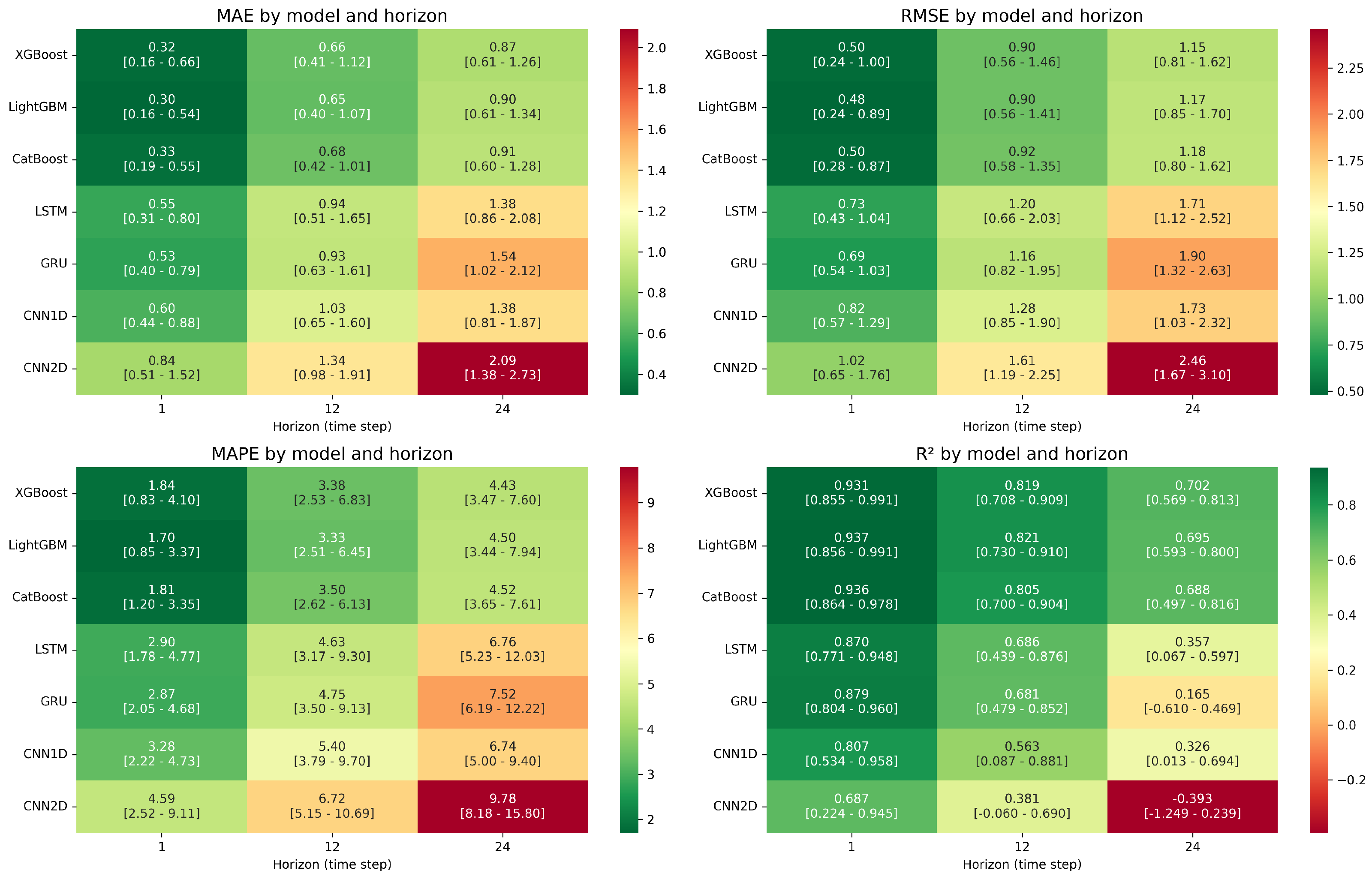
Figure 6 visually confirms this superiority through a color-coded heatmap, where these models occupy the lightest regions (indicating better performance). Each cell presents results in the format: mean [minimum – maximum], providing a comprehensive view of performance distribution.
XGBoost: For short-term predictions (1 time step), XGBoost achieves excellent accuracy with MAE ranging from to (mean: ), RMSE from to 1.00 (mean: ), MAPE from % to % (mean: %), and R2 from to (mean: ). Performance remains robust at medium-term horizons (12 time steps) with MAE from to (mean: ), RMSE from to (mean: ), MAPE from % to % (mean: %), and R2 from to (mean: ). For long-term predictions (24 time steps), XGBoost maintains acceptable performance with MAE from to (mean: ), RMSE from to (mean: ), MAPE from % to % (mean: %), and R2 from to (mean: ).
LightGBM: This model performs comparably to XGBoost with short-term MAE from to (mean: ), RMSE from to (mean: ), MAPE from % to % (mean: %), and R2 from to (mean: ). Medium-term metrics show slight deterioration with MAE from to (mean: ), RMSE from to (mean: ), MAPE from % to % (mean: %), and R2 from to (mean: ). Long-term prediction maintains robustness with MAE from to (mean: ), RMSE from to (mean: ), MAPE from % to % (mean: %), and R2 from to (mean: ).
CatBoost: Performance metrics are consistent with other Gradient Boosting models, showing short-term MAE from to (mean: ), RMSE from to (mean: ), MAPE from % to % (mean: %), and R2 from to (mean: ). Medium-term predictions show expected degradation with MAE from to (mean: ), RMSE from to (mean: ), MAPE from % to % (mean: %), and R2 from to (mean: ). Long-term metrics remain competitive with MAE from to (mean: ), RMSE from to (mean: ), MAPE from % to % (mean: %), and R2 from to (mean: ).
6.2.2. Recurrent Neural Models
LSTM and GRU models demonstrate intermediate performance, positioned between Gradient Boosting algorithms and convolutional models.
Figure 6 displays these models with middle-range shading, indicating their moderate effectiveness with notable performance degradation as prediction horizons increase.
LSTM: Short-term predictions show moderate accuracy with MAE from to (mean: ), RMSE from to (mean: ), MAPE from % to % (mean: %), and R2 from to (mean: ). Medium-term performance decreases with MAE from to (mean: ), RMSE from to (mean: ), MAPE from % to % (mean: %), and R2 from to (mean: ). Long-term prediction quality deteriorates significantly with MAE from to (mean: ), RMSE from to (mean: ), MAPE from % to % (mean: %), and R2 declining to between and (mean: ).
GRU: Performance follows similar patterns to LSTM with short-term MAE from to (mean: ), RMSE from to (mean: ), MAPE from % to % (mean: %), and R2 from to (mean: ). Medium-term metrics worsen with MAE from to (mean: ), RMSE from to (mean: ), MAPE from % to % (mean: %), and R2 from to (mean: ). Long-term performance drops substantially with MAE from to (mean: ), RMSE from to (mean: ), MAPE from % to % (mean: %), and R2 declining to between and (mean: ).
6.2.3. Convolutional Models
CNN1D and CNN2D consistently demonstrate the lowest performance across all tested algorithms, particularly for longer prediction horizons.
Figure 6 highlights this trend with darker shading in cells corresponding to these models, indicating higher error metrics.
CNN1D: Short-term predictions show MAE from to (mean: ), RMSE from to (mean: ), MAPE from % to % (mean: %), and R2 from to (mean: ). Medium-term performance degrades with MAE from to (mean: ), RMSE from to (mean: ), MAPE from % to % (mean: %), and R2 from to (mean: ). Long-term predictions show further deterioration with MAE from to (mean: ), RMSE from to (mean: ), MAPE from 5.00% to % (mean: %), and R2 from to (mean: ).
CNN2D: This model exhibits the poorest overall performance with short-term MAE from to (mean: ), RMSE from to (mean: ), MAPE from % to % (mean: %), and R2 from to (mean: ). Medium-term metrics show pronounced degradation with MAE from to (mean: ), RMSE from to (mean: ), MAPE from % to % (mean: %), and R2 from to (mean: ). Long-term performance collapses further with MAE from to (mean: ), RMSE from to (mean: ), MAPE from % to % (mean: %), and R2 from to (mean: ), indicating performance worse than a simple mean-based prediction model.
6.3. Analysis of Performance Degradation by Horizon
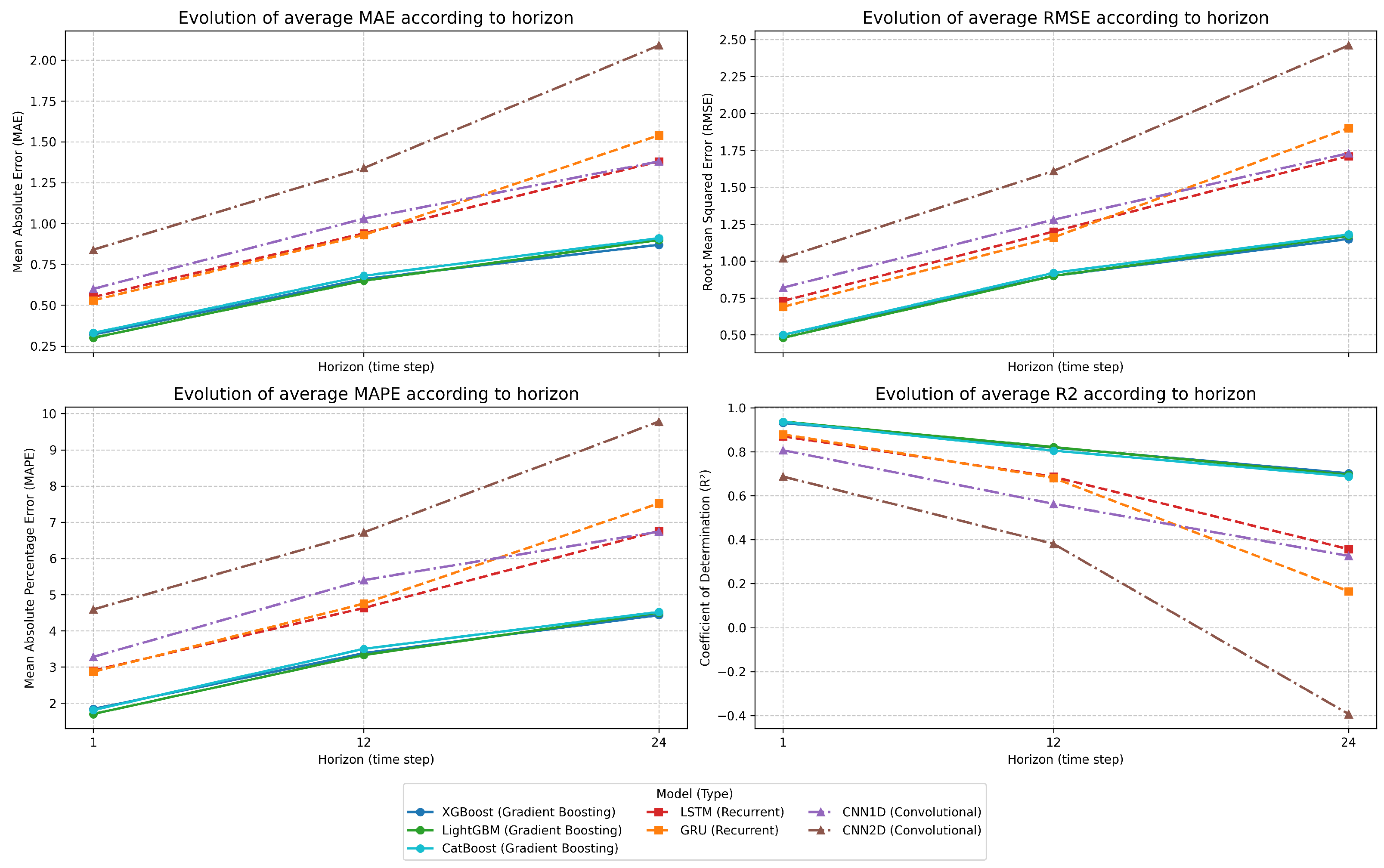
Figure 7 highlights a common phenomenon across all models: performance degradation with the increase in prediction horizon. However, this degradation is not uniform across different algorithm families.
Gradient Boosting models exhibit the lowest degradation, with an increase in mean MAE of approximately
between horizons 1 and 24 for XGBoost (from
to
). This robustness is reflected in the moderately sloped curves in
Figure 7, indicating a better ability to maintain accurate predictions over extended horizons.
Recurrent models (LSTM and GRU) show intermediate degradation, with a rise in mean MAE of
for LSTM (from
to
) and
for GRU (from
to
) between horizons 1 and 24. Their curves in
Figure 7 display a steeper slope, particularly between horizons 12 and 24.
Convolutional models experience the most significant degradation, with the mean MAE increase reaching
for CNN1D (from
to
) and
for CNN2D (from
to
) between horizons 1 and 24. This substantial decline is especially visible in
Figure 7, where the corresponding curves have the steepest slope.
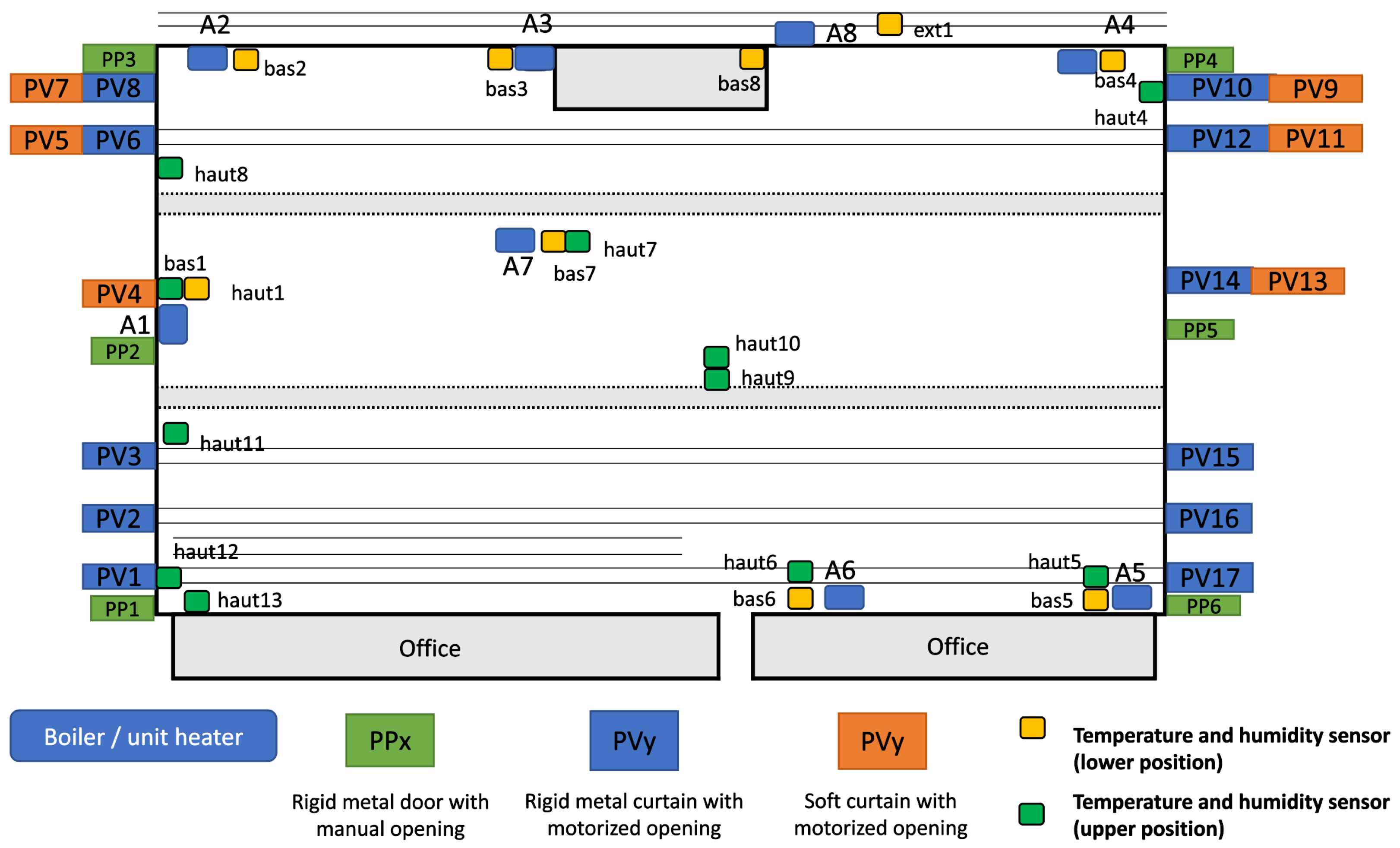
6.4. Impact of Sensor Location on Prediction Accuracy
An analysis of the prediction results highlights the significant influence of sensor placement within the studied industrial building on the performance of the temperature prediction models. Specifically, sensors tempBAS2 and tempBAS4 exhibit the poorest prediction accuracy. This degradation can be attributed to their proximity to vehicle doors, which are frequently opened. The frequent opening of these doors creates air currents that introduce additional thermal variability, disrupting the ability of the models to accurately predict temperature changes. Consequently, the metrics for these sensors show consistently higher errors compared with others. It is important to note that the temperature sensors used in this study have a precision of . Therefore, any prediction error below this threshold is considered reliable, as it remains within the bounds of sensor accuracy. This consideration helps contextualize the observed model performance, especially in distinguishing between meaningful prediction discrepancies and those that fall within the expected measurement uncertainty. In contrast, sensors tempBAS3, tempBAS6, and tempBAS7 demonstrate excellent prediction accuracy. These sensors are located at the center of the building, far from the disruptive effects of the vehicle doors. Furthermore, their central positions are surrounded by other hot air generator units, which contribute to more stable and homogeneous thermal conditions. This configuration minimizes external disturbances and enhances the precision of the models. Lastly, sensor tempBAS8 also achieves above-average prediction accuracy, which is likely due to its placement within a small, enclosed room. The closed environment reduces the influence of external climatic variations and air currents, resulting in more predictable thermal behavior and improved model performance. This analysis underscores the importance of sensor location in industrial temperature prediction tasks. The proximity to external disturbances, such as open doors, can significantly degrade prediction performance, whereas central and enclosed locations provide favorable conditions for achieving higher accuracy.
Feature importance analysis conducted on the Gradient Boosting models confirms these observations, consistently ranking external temperature (tempEXT) as the most influential variable, followed by heating relay states (comRELAIS) and sensor location factors. This analysis validates that the models appropriately capture the physical relationships governing the building’s thermal behavior.
6.5. Superiority of Traditional Models for Extreme Thermal Characteristics in Industrial Buildings
The building in question is characterized by two extreme thermal features: almost no thermal inertia and an overpowered heating system with forced-air diffusion. These factors create an atypical thermal behavior with rapid and large fluctuations, resulting in a highly responsive temperature profile.
An in-depth analysis highlights a counterintuitive phenomenon: the most recent and sophisticated learning models, particularly complex neural network architectures (LSTM, GRU, CNN1D, and CNN2D), perform significantly suboptimally compared with traditional Gradient Boosting algorithms. This observation warrants a detailed analysis in the context of the unique thermal characteristics of the studied industrial building.
While deep neural networks are theoretically designed to capture complex temporal dependencies and subtle spatial patterns, they paradoxically prove less suitable in this context. Several factors may explain this.
Overfitting to Slow Dynamics: LSTM and GRU networks, designed to model long-term dependencies, tend to overparameterize temporal relationships in an environment with nearly instantaneous changes. The mean MAE increases from to for LSTM and from to for GRU between horizons 1 and 24, a significantly steeper degradation compared with Gradient Boosting models (from to for XGBoost).
Inadequacy of Spatial Convolutions: CNN2D models, particularly ineffective with a catastrophic mean R2 of at the 24-time-step horizon, attempt to identify spatial thermal propagation patterns in an environment where forced ventilation rapidly homogenizes the temperature, making such patterns non-existent or irrelevant. The poor performance of CNN2D models cannot be attributed to inadequate training, as rigorous safeguards including early stopping, regularization, and controlled parameter counts were implemented. Instead, the fundamental mismatch between CNN spatial assumptions and the building’s instantaneous thermal response characteristics explains this performance degradation.
Excessive Complexity for Simple Relationships: The building’s thermal profile, dominated by heating power and the absence of inertia, presents almost linear relationships between input variables (heating power, external temperature) and the resulting temperature. Gradient Boosting models, using decision tree ensembles, efficiently capture these straightforward relationships without the unnecessary complexity introduced by deep neural networks.
An analysis of
Figure 6 reveals that convolutional models, particularly CNN2D, occupy the darkest regions of the heatmap for all metrics, confirming their relative inadequacy for this industrial thermal prediction task. The analysis of the various metrics presented in
Figure 6 provides a deeper understanding of model performance.
The MAE and RMSE show similar trends, with consistently higher values for RMSE due to its sensitivity to large errors. These two metrics confirm the superiority of Gradient Boosting models, followed by recurrent models and then convolutional models.
The MAPE offers a complementary perspective by normalizing errors relative to observed values. This metric reveals that even the most accurate models (XGBoost and LightGBM) exhibit relative errors reaching mean values of % and %, respectively, for the 24-time-step horizon. In contrast, the CNN2D reaches a mean MAPE of %, confirming its low accuracy.
The R2 assesses the models’ ability to explain data variance. Gradient Boosting models maintain a mean R2 above even at the 24-time-step horizon, whereas recurrent models see their mean R2 drop below at this horizon. The CNN2D shows a negative mean R2 at the long horizon, indicating its inability to capture long-term thermal trends.
6.6. Generalizability and Applicability Framework
The findings of this study are specifically tied to the thermal characteristics of the investigated industrial building, which exhibits two extreme features: minimal thermal inertia and an overpowered forced-air heating system. However, the methodological approach and key insights can be extended to other industrial facilities sharing similar thermal dynamics.
Applicability Criteria: The superiority of Gradient Boosting algorithms over deep learning approaches is expected to generalize to industrial buildings characterized by: low thermal inertia due to minimal insulation and high ceiling heights, forced-air heating systems with rapid thermal response, frequent thermal disruptions from operational activities (door openings, equipment cycling), and spatially distributed heating sources creating localized thermal zones rather than uniform temperature fields.
Conversely, buildings with high thermal mass, radiant heating systems, or strong spatial thermal gradients may benefit more from deep learning approaches, particularly CNN architectures designed to capture spatial relationships. Similarly, facilities with complex temporal thermal patterns or significant thermal lag effects might favor recurrent neural network architectures.
Validation Considerations: The proposed algorithmic selection framework requires validation across diverse industrial contexts. Key factors for assessment include: building envelope characteristics (insulation, thermal mass), HVAC system type (forced-air, radiant, mixed), operational patterns (continuous vs. intermittent), and external disturbance frequency. A preliminary assessment based on these criteria can guide initial algorithm selection, followed by empirical validation using the comparative methodology demonstrated in this study.
Sensor Placement Implications: The significant impact of sensor location on prediction accuracy (
Section 6.4) suggests that the generalizability framework must also consider facility layout and sensor positioning strategies. Industrial buildings with similar thermal characteristics but different spatial configurations may require adapted sensor networks to achieve comparable prediction performance.
Ultimately, the criteria outlined above define the scope for the direct transfer of our results. However, it is essential to distinguish the limited generalizability of these specific findings from the broad applicability of our comparative methodology. The systematic protocol for data preparation, model training, and multi-horizon evaluation demonstrated in this study provides a robust and replicable framework. This framework can guide practitioners in selecting the optimal predictive algorithm for their own facilities, even those with thermal characteristics that differ significantly from our case study.
7. Conclusions
This comparative study rigorously evaluated the performance of various artificial intelligence algorithms for temperature prediction within an industrial building, with a clear objective: to optimize thermal management.
The key findings of this comparative analysis demonstrate the superior performance of Gradient Boosting algorithms, notably XGBoost and LightGBM, for temperature prediction in the studied industrial building. These models consistently exhibited the lowest prediction errors, as measured by the RMSE, the MAE, and the MAPE, when compared with the other evaluated algorithms, including LSTM and convolutional neural networks (CNNs). Furthermore, they achieved higher R2, indicating a better ability to explain the variance in the temperature data. While the precise values of these metrics are detailed in the results sections, the overarching trend highlights the enhanced accuracy and reliability of the predictions provided by XGBoost and LightGBM for short- and mid-term thermal management within this specific industrial context.
This study contributes several novel insights: systematic comparison of seven AI algorithms on real industrial data, empirical demonstration of Gradient Boosting superiority over deep learning in low thermal inertia environments, quantitative analysis of sensor placement impact on prediction accuracy, and methodological framework for algorithm selection based on building thermal characteristics.
The hyperparameter tuning strategy employed in this study demonstrates that pragmatic, consistent approaches can provide meaningful model comparisons while respecting computational constraints typical of industrial settings. By prioritizing methodological consistency over exhaustive optimization, the study avoided the selection bias that can occur when models receive unequal tuning effort, ensuring that our comparative results reflect genuine algorithmic differences rather than optimization artifacts.
These results underscore the crucial importance of carefully selecting models based on the specific thermal characteristics of the building. In this instance, Gradient Boosting approaches proved particularly effective at capturing the immediate causal relationships that define the industrial environment’s thermal dynamics. This finding challenges the common assumption that deep learning architectures are systematically superior for predictive tasks, demonstrating instead the critical importance of architectural alignment with physical system properties.
The superiority of traditional models in this context can be attributed to several factors.
Simplicity of Thermal Relationships: The studied industrial building exhibits a thermal dynamic primarily driven by immediate factors such as heating power and external temperature, with minimal influence from thermal inertia. This characteristic favors models capable of efficiently capturing direct and straightforward relationships between input variables and internal temperature. The building’s thermal characteristics favor direct variable relationships over complex derived features, as confirmed by preliminary feature selection tests that showed no performance improvement with reduced feature sets.
Robustness to Rapid Variations: Gradient Boosting models demonstrated superior adaptability to the rapid temperature fluctuations characteristic of this industrial environment, unlike neural network models, which tend to overfit or misinterpret these variations.
Computational Efficiency: In an industrial setting using standard multi-service infrastructure, traditional models offer significant advantages with inference times typically under 10 ms, well within the requirements for thermal control systems operating on 5 min cycles. This computational efficiency makes them particularly suitable for real-time industrial deployment.
Interpretability: Gradient Boosting models provide better interpretability of results through native feature importance analysis, which consistently identified external temperature, heating relay states, and sensor positioning as the primary predictive factors. This transparency is crucial in industrial environments where understanding the factors influencing predictions is essential for decision-making and process optimization.
Broader Implications and Future Research: While this study focuses on a specific industrial building with extreme thermal characteristics, the methodological framework provides a foundation for algorithm selection in broader industrial contexts. The key insight—that model architecture must align with physical system properties—extends beyond the specific case study to inform predictive modeling strategies across diverse industrial facilities.
Future research should investigate the proposed applicability framework across industrial buildings with varying thermal characteristics, HVAC configurations, and operational patterns. Particular attention should be given to developing automated assessment tools that can rapidly classify building thermal dynamics and recommend appropriate algorithmic approaches based on easily measurable facility characteristics.
Future research could also employ advanced interpretability techniques, such as SHAP (SHapley Additive exPlanations) analysis, to gain even finer-grained insights into individual prediction drivers.
The integration of these predictive models within broader Industry 4.0 ecosystems represents another avenue for investigation, particularly regarding real-time model adaptation and multi-building optimization strategies. Such developments could enable the scalable deployment of intelligent thermal management systems across large industrial portfolios.
Moreover, these results have significant implications for the integration of artificial intelligence within the context of Industry 4.0 and energy efficiency. The ability to accurately predict temperature enables proactive thermal management, potentially reducing energy consumption and ensuring optimal conditions for production and product quality. In an increasingly regulatory and societal landscape focused on reducing carbon footprint (as exemplified by the ELAN law in France), the adoption of such technologies represents a significant lever.
On a practical level, this study suggests that industrial companies should seriously consider the implementation of Gradient Boosting algorithms for temperature prediction within their infrastructures. The integration of these models with existing BACS could lead to a significant optimization of HVAC systems, yielding concrete economic and environmental benefits. The results obtained underscore the importance of a data-driven approach to improve energy efficiency in the industrial sector.
This research contributes to the understanding of the potential of AI for industrial thermal management, highlighting the effectiveness of Gradient Boosting algorithms and paving the way for practical applications for a more sustainable and efficient industry.


