Optimization of Large Deformable Elastic Braces in Two-Degrees-of-Freedom Systems

Abstract

This study presents a computational approach to optimize the stiffness distribution of large deformable elastic braces (LDEBs), which possess a high elastic deformation capacity and are designed to enhance the seismic performance of building structures. An optimization problem was formulated to minimize the seismic response of two-story buildings modeled as multi-degree-of-freedom systems, in which both the building frame and the LDEBs were represented by spring elements. Seismic responses under earthquake excitations were evaluated through time-history analyses. Particle swarm optimization (PSO) was employed to determine the optimal stiffness ratios of LDEBs that minimize the maximum story drift. Extensive round-robin analyses were conducted to verify the validity of the PSO results, generating response surfaces that mapped the maximum story drift against the LDEBs’ stiffness under three different earthquake records. The analysis revealed that the optimal solutions obtained from the PSO coincided with the global minimum identified in the round-robin response surfaces. These results confirm the effectiveness of the proposed optimization framework and demonstrate the potential of LDEBs for enhancing seismic resilience in structural designs.

1. Introduction

Current Japanese earthquake resistance standards permit building structures to be damaged during large earthquakes while protecting human life. However, there is an increasing demand for structural members to reduce damage and maintain the value of their properties, even in large earthquakes. Due to this background, various seismic response control technologies [1,2,3,4,5,6] have been implemented in the last decades, including optimization-based approaches for stiffness and damping distribution [7,8]. Metallic-yielding dampers [9,10] are widely used in Japanese buildings and are generally intended to dissipate seismic energy before the material of the main frame yields or buckles. While they allow the main frame to remain elastic under major earthquakes, this assumption may not be effective for severe motions beyond the design level [11,12]. Consequently, large residual deformation may occur, disrupting the continuous usability of buildings.

The LDEBs proposed by Sawada are processed steel plates with special shapes that have a larger elastic limit than normal braces due to their flexible performance. In structures with LDEBs, the elastic restoring force works until LDEBs yield; therefore, the structure obtains additional post-yielding stiffness even when the main frame members yield. Past research conducted monotonic tension loading experiments on LDEBs to verify their elastic yielding deformation, and seismic response analysis frameworks clarified their effectiveness [11].

However, two key research gaps remain unaddressed. First, while metaheuristic optimization techniques have been widely applied to conventional dampers and bracing systems, limited attention has been given to optimizing the stiffness distribution of LDEBs. Second, prior studies often relied solely on optimization algorithms without systematically validating global optimality across broad seismic scenarios.

To fill this gap, this work presents a new hybrid optimization framework that integrates particle swarm optimization (PSO) with round-robin response surface analysis. This dual approach identifies globally optimal stiffness configurations for LDEBs in multi-degree-of-freedom (MDOF) systems and verifies the solutions’ robustness under different seismic inputs. The importance of these studies is in their applicability worldwide and the validation of their results via experimental work, formally establishing the leading-edge technology for the robust optimization of LDEBs that can be applied with confidence to enhance the seismic safety of structural buildings.

Recent studies have optimized dampers and braces using metaheuristic algorithms [13,14,15], but the optimum stiffness distributions of LDEBs in multi-story buildings are still unknown. Previous research [16] confirmed the elastic limit and post-yielding performance of large deformable elastic plates (LDEPs), validating their potential in seismic mitigation. This study advances the practical use of LDEBs by optimizing their stiffness distribution in two-story structural models.

While PSO has been applied to optimize damper placement and stiffness in seismic design, limited attention has been given to the unique behavior of LDEBs, whose highly nonlinear elastic characteristics require careful optimization. The interaction between MDOF systems and the variable stiffness levels of LDEBs has not been systematically explored. This study introduces a hybrid framework combining PSO and round-robin response surface analyses. PSO enables efficient global search, while round-robin analysis validates the results through comprehensive response surface mapping, enhancing reliability in capturing global optima and structural performance trends across varying seismic intensities. This combination ensures robust, optimized stiffness configurations across different seismic scenarios.

This study aimed to obtain the optimum stiffness distribution of LDEBs in MDOF systems as useful knowledge for structural designs. Specifically, this study considered two-degrees-of-freedom (2-DOF) systems that represented two-story buildings in the first stage of the research. First, the optimization problem that finds the optimum stiffness of LDEBs was formulated and solved using the PSO method, which has been successfully applied in seismic design optimization [17,18]. Next, a round-robin analysis of 2-DOF models with a wide range of secondary stiffness ratios subjected to three different earthquake types was carried out. Through comparison, the PSO solution corresponded to the global optimum identified via the round-robin analysis.

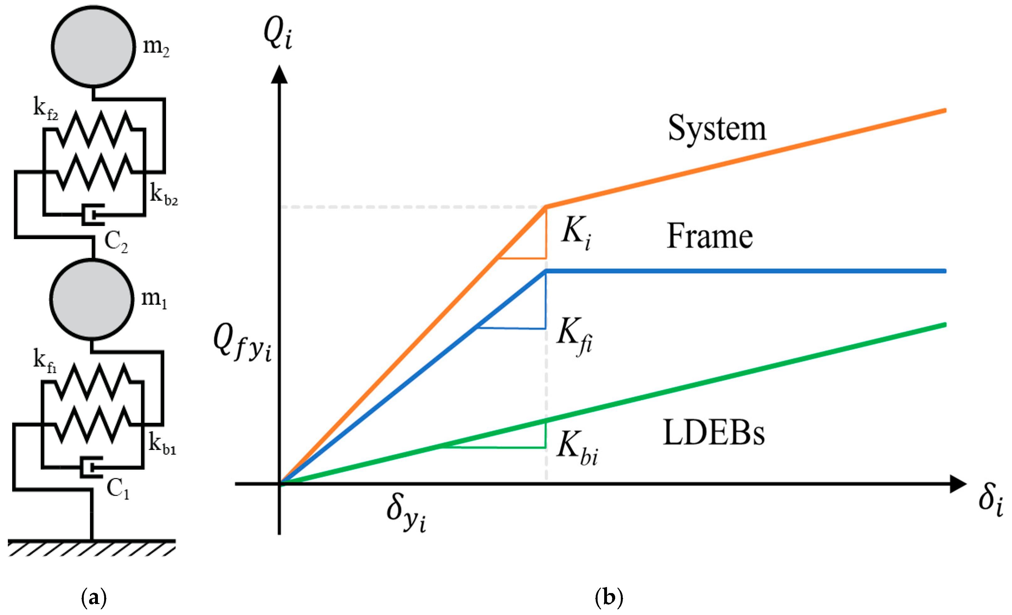
2. Target Models

This study demonstrates the performance of 2-DOF systems, as shown in Figure 1. K_fi and K_bi denote the stiffness of the main frame and LDEBs in the ith story, respectively. Therefore, the ith overall stiffness (K_i) and stiffness ratio (α_i) of the LDEBs against the main frame can be expressed as

$$K_i=K_{fi}+K_{bi}$$

(1)

$${\alpha }_i=K_{bi} / K_{fi}$$

(2)

The damping coefficient of the ith story’s dashpot C_i was assumed to be proportional to K_i. The mechanical properties of each story are shown in

Table 1. Mechanical properties for two-story main frames.

Data	1st Story	2nd Story
Weight, $\mathit{W}$	1000 kN	1000 kN
$\mathrm{Yielding} \mathrm{story} \mathrm{shear} \mathrm{force}, Q_{y_i}$	600 kN	378 kN
$\mathrm{Yielding} \mathrm{deformation}, {\delta }_{y_i}$	2 cm	2 cm
$\mathrm{Story} \mathrm{stiffness}, K_{f_i}$	300 kN/cm	189 kN/cm

. The yield shear force in each story was calculated from the required strength against the level 2 seismic force specified by the Building Center of Japan (BCJ) code [19].

This research used a simplified 2-DOF system as a preliminary step to systematically explore the fundamental optimization behavior of LDEBs under seismic excitation. This enabled the unambiguous identification of dominant parameters and nonlinear responses, as well as the interactions between LDEBs and the primary frame components, while the computational cost was affordable. Even though a 2-DOF system does not fully reflect the complexity of multi-story building structures compared with real situations, it offers a well-defined test bed to verify the efficiency of the PSO and round-robin hybrid optimization scheme. The understanding obtained here provides a solid grounding for generalization to full multi-story MDOF models, which consider further aspects, including higher-mode effects, inhomogeneous stiffness distributions, and realistic combinations of load effects. Further research will apply the optimization methodology to taller structures with enhanced damping models and compare it with a more detailed structural representation and experimental data to validate the framework.

3. Natural Period and Mode Shapes

In earthquake engineering, each structure possesses a unique natural period governing its response to lateral forces such as ground motion during earthquakes. This inherent period, often identified through eigenvalue analysis, is crucial for design as it determines how a building sways in response to shaking. An effective seismic response relies on harmonizing forces with this natural period, allowing the building to resonate and efficiently dissipate energy.

Eigenvalue analysis helps us understand the dynamic behavior of 2-DOF systems.

Table 2. Natural periods.

Mode	1st Mode	2nd Mode
Without LDEBs	0.64	0.26
$\mathrm{With} \mathrm{LDEBs} (K_{b1}$$=90 \mathrm{kN}/\mathrm{cm}; K_{b2}$ = 56.7 kN/cm)	0.56	0.23
Change (%)	−12.50	11.54

presents the results of this analysis, highlighting the natural periods of different modes. Figure 2 provides the mode shapes, visually depicting the deformation patterns of the structure at each natural period. As shown, the first mode has a natural period of 0.56 s, while the second mode vibrates faster, with a period of 0.23 s. This knowledge of the 2-DOF system’s natural periods and mode shapes forms the foundation for understanding how it interacts with earthquake forces.

4. Response Spectrum

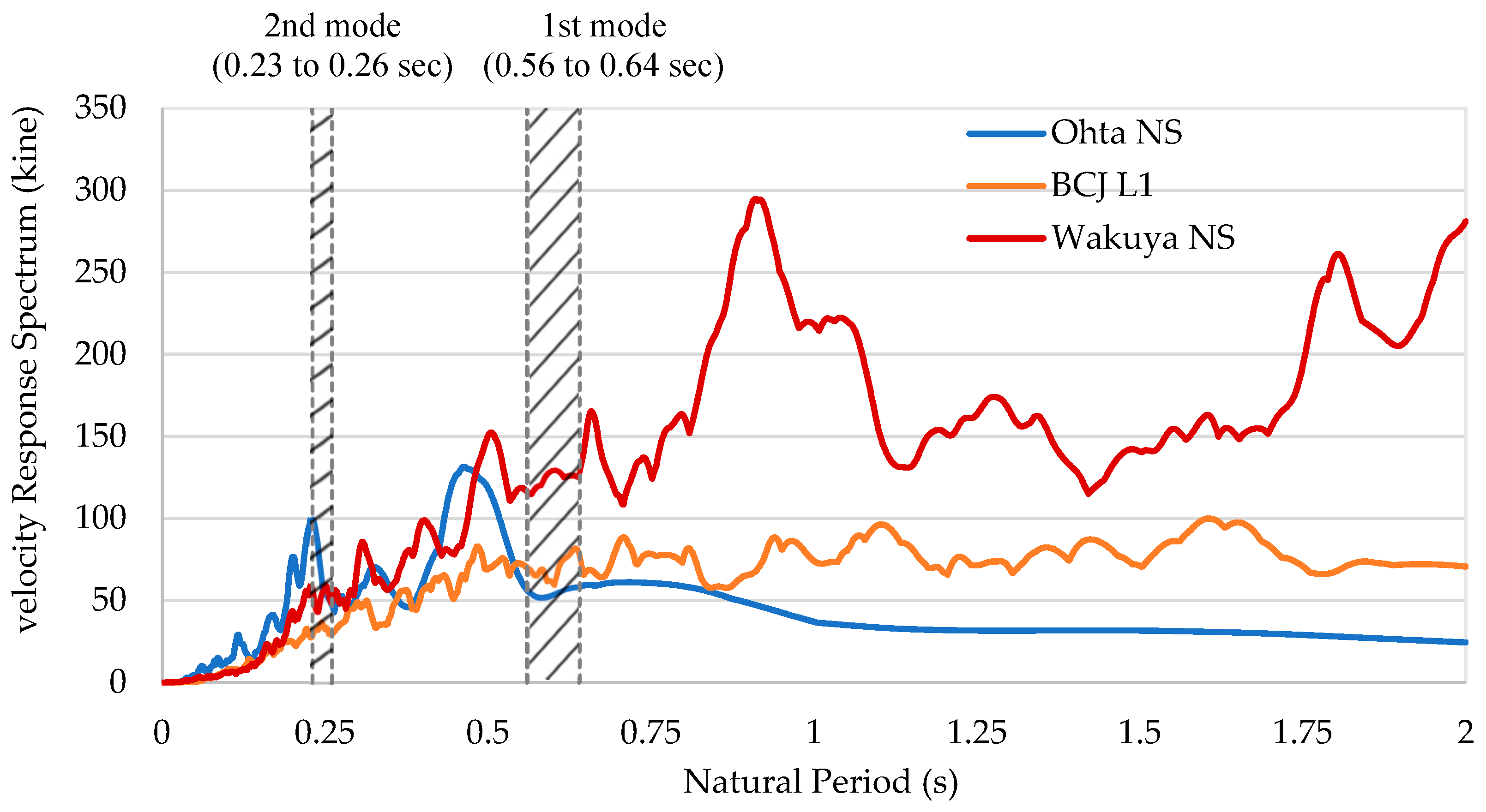
Buildings, including our simplified 2-DOF models, are not passive recipients of earthquake force. Their response varies based on both their own natural periods and the earthquake’s characteristics. To account for this dynamic interplay, engineers utilize response spectrum graphs. These graphs illustrate the maximum responses (e.g., displacement and velocity) a building experiences at different periods (or frequencies), essentially covering a range of potential earthquake scenarios. The velocity response spectrum is displayed in Figure 3. The selected earthquake records exhibit distinct frequency characteristics. At a natural period of approximately 0.5 s, Ohta NS produced a peak response of approximately 112 kine, whereas BCJ-L1 maintained a relatively constant response near 70 kine. However, for a natural period of approximately 0.9 s, Wakuya NS showed a response at a much higher level, which was approximately estimated to be 285 kine. Hence, these three earthquakes were chosen so that their frequency contents and seismic intensities would cover a wide range of parameters for a more complete evaluation of the optimization performance of LDEBs in different seismic environments.

Figure 3 displays a velocity response spectrum, plotting the maximum expected velocity response (kine) against the natural period of the structure. This spectrum directly informs our understanding of how the two-story model behaves in different earthquake scenarios. By comparing the natural periods identified in Table 2 and Figure 2 with the response spectrum in Figure 3, we can achieve the following:

• Predict the dominant response. If the natural period falls within a peak region of the spectrum, that specific frequency will likely cause significant vibrations in the building.
• Understand the building behavior using the response spectrum. Two-degrees-of-freedom models react differently during earthquakes, depending on their natural vibration periods and the type of earthquake. To understand this, engineers use response spectrum graphs. These show the maximum shaking velocity a model might experience at different natural periods.
• Optimize design interventions. Knowing the expected response allows engineers to tailor reinforcements and energy dissipation strategies to effectively address the anticipated earthquake forces, considering the specific limitations and advantages of the 2-DOF model.

Incorporating both eigenvalue analysis and response spectrum analysis into the design process is crucial for ensuring an earthquake-resistant structure. Engineers can create effective strategies to minimize damage and safeguard occupants by understanding the 2-DOF model’s natural periods and how it interacts with different earthquake frequencies.

5. Large Deformable Elastic Braces (LDEBs)

LDEBs are devices that never yield, even when subject to large deformations during major earthquakes [11]. In structures equipped with LDEBs, the elastic restoring force generated by these devices can improve the seismic response to major earthquakes [20]. Our study confirmed that LDEBs exhibit elastic properties. Figure 4 and Figure 5 illustrate LDEBs and their capability for substantial elastic deformation. The corresponding natural periods of the system with these devices are listed in Table 2. However, traditional braces have limitations in adjusting their elastic limits. In contrast, LDEBs possess a large yielding capacity and can dynamically modify their elastic limits, making them more effective in mitigating seismic responses across a wider range of earthquake intensities.

6. Formulation of Optimization Problem

This study aimed to determine the optimal stiffness distribution of LDEBs in MDOF systems, which minimizes the maximum story drift response under seismic excitation. The LDEBs are represented as elastic spring elements installed in parallel with the primary frame elements at each story level. The optimization problem can be expressed in the following mathematical form:

$$\underset{\alpha }{\min } \underset{i=1,2}{\max }\left\{{\delta }_{yi}\left(\alpha \right)\right\}$$

(3)

where $\alpha =\left({\alpha }_1,{\alpha }_2\right)$ represents the stiffness ratio of LDEBs to the main frame at each story. ${\delta }_i\left(\alpha \right)$ denotes the maximum story drift at story iii, obtained via seismic response time-history analysis. The design variables ${\alpha }_i$ are dimensionless and bounded within practical ranges based on preliminary structural considerations and the LDEBs’ properties.

The search space for the design variables is constrained as

$$0\hspace{0.17em}\hspace{0.17em}\le \hspace{0.17em}\hspace{0.17em}{\alpha }_i\hspace{0.17em}\le \hspace{0.17em}0.3$$

This upper bound (30%) reflects realistic limits on the additional stiffness that can be introduced by LDEBs without compromising constructability or cost efficiency, or introducing excessive stiffness that may amplify higher-mode responses.

The maximum story drift serves as the objective function, since excessive drift directly correlates with structural and non-structural damage during seismic events. The solution obtained aims to minimize the worst-case drift across both stories, enhancing seismic resilience.

7. Condition of Seismic Response Analysis

The seismic response analysis was performed iteratively to find the stiffness of a large deformable spring in each story. For the numerical solution of the equation of motion, the Newmark-β method was used with β = 0.25, the numerical integration time interval was 0.001 (s), the damping type was stiffness proportional damping, and the damping constant was 2% [19].

In this study, the damping was assumed to be proportional to the overall stiffness of each story, including the main frame and LDEBs. This assumption compared the various stiffness setups consistently and simplified the numerical modeling as well. Although damping that is proportional to stiffness is standard for the analysis of the seismic response of MDOF systems, it may not model the complicated energy dissipation mechanisms that contribute to the LDEBs, which can show material hysteretic and geometrical nonlinearities while undergoing large deformations. The potential implications of this simplification are discussed in the Limitations section.

8. Ground Motion Data

After a meticulous selection process, three ground motion records, including two real-world recordings and one artificial simulation, were obtained.

Table 3. Input seismic wave data.

Earthquake Name	Shimane 2018	Artificial	Tohoku 2011
Station	Ohta NS (SMN006)	BCJ–L1	Wakuya NS (JMA)
Seismic record duration time (s)	50	60	360
Maximum ground acceleration (gal)	477	207	406

provides a concise overview of the key characteristics of these records. The ground acceleration for each individual record is presented in Figure 6. Figure 3 visualizes the 2% damped velocity response spectra for each record, along with the placement of the two-story systems modeled as 2-DOF systems within these spectra. This research utilized seismic waves at two distinct scaled velocity levels to facilitate a comprehensive analysis: 50 kine and 90 kine. Detailed information regarding these levels is available in

Table 4. Seismic multiplication factor.

Solutions	Maximum Acceleration (gal)	Maximum Velocity (kine)	Amplitude Multiplication Factor
			50 kine	90 kine
Ohta NS	477	22.75	2.198	3.956
BCJ–L1	207	33.75	1.481	2.667
Wakuya NS	406	85.22	0.587	1.056

. The velocity level of 50 kine corresponded to the major earthquake level in the current Japanese seismic code [21]. The velocity level of 90 kine was slightly above the largest value of strong motions from 79 moderate magnitude (5.9 ≥ Mw) earthquakes that caused various degrees of impact on humans and built environments in Japan between 1996 and 2019, after the start of K-NET and KiK-net [22].

9. Optimization Methods

A two-stage hybrid computational framework was employed to effectively solve the formulated optimization problem, combining the global search capability of PSO with the verification robustness of round-robin response surface analysis.

9.1. Phase 1: Particle Swarm Optimization (PSO)

PSO is a population-based metaheuristic optimization algorithm, which is inspired by flocks’ social behavior. Each particle moves toward its last best local position (P_best) and the global best position (G_best) in the swarm to obtain the best solution [23,24,25]. We minimized the problem such that

$$P_{bes{t}_i}\hspace{0.17em}=\hspace{0.17em}\underset{k=1,2\dots ,t}{\min } \left\{f\left(x_i^k\right)\right\},\hspace{0.17em}\hspace{0.17em}\hspace{0.17em}\hspace{0.17em}\hspace{0.17em}\hspace{0.17em}\hspace{0.17em}\hspace{0.17em}\hspace{0.17em}\hspace{0.17em}\hspace{0.17em}\hspace{0.17em}\hspace{0.17em}\hspace{0.17em}\mathrm{where}\hspace{0.17em}i\in \hspace{0.17em}\left\{1,\hspace{0.17em}2,\dots ,N\right\}$$

(4)

$$G_{bes{t}_i}\hspace{0.17em}=\hspace{0.17em}\underset{k=1,\hspace{0.17em}\hspace{0.17em}2\dots ,\hspace{0.17em}t}{\min }\hspace{0.17em}\left\{f\left(x_i^k\right)\right\},\hspace{0.17em}\hspace{0.17em}\hspace{0.17em}\hspace{0.17em}\hspace{0.17em}\hspace{0.17em}\hspace{0.17em}\hspace{0.17em}\hspace{0.17em}\hspace{0.17em}\hspace{0.17em}\hspace{0.17em}\hspace{0.17em}\hspace{0.17em}\hspace{0.17em}\mathrm{where}\hspace{0.17em}\hspace{0.17em}i\in \hspace{0.17em}\hspace{0.17em}\left\{1,\hspace{0.17em}2,\dots ,N\right\}$$

(5)

where i and N represent the particle index and the total number of particles, t denotes the current iteration number, f is the fitness value of the function, and P indicates the particles’ position. In this study, each particle represents a candidate solution vector $\alpha =\left({\alpha }_1,{\alpha }_2\right)$. The particles explore the defined solution space according to the following velocity and position update rules, detailed as follows:

$$V_i^{\left(t+1\right)}=\omega V_i^{\left(t\right)}+c_1{r}_1(P_{bes{t}_i}-x_i^{\left(t\right)})+c_2{r}_2(G_{bes{t}_i}-x_i^{\left(t\right)})$$

(6)

$$x_i^{(t+1)}\hspace{0.17em}=\hspace{0.17em}{x}_i^{\left(t\right)}\hspace{0.17em}+\hspace{0.17em}{v}_i^{\left(t+1\right)}$$

(7)

where $V_i^{\left(t\right)}$ and $x_i^{\left(t\right)}$ are the velocity and position of the particle. $c_1$ and $c_2$ are cognitive and social acceleration coefficients, respectively. $r_1,r_2$ are independent uniformly random variables between 0 and 1.

Since the inertia weight concept was proposed, a linear time-variant inertia weight was proposed to enhance the PSO algorithm’s performance [26,27,28,29]. The role of the linear time-variant inertia weight ${\omega }_1^t$ is presented by the following equation:

$${\omega }_1^{\left(t\right)}={\omega }_{ini}-\left({\displaystyle \frac{i}{i_{max}}}\right)({\omega }_{ini}-{\omega }_{fin})$$

(8)

where the initial value, ${\omega }_{ini}=1.0$, the final value, ${\omega }_{fin}=0.0,$ and $i_{max}$ is the maximum number of iterations.

PSO efficiently searches the defined solution space to identify near-optimal stiffness ratios that minimize the maximum story drift for each seismic input considered.

9.2. Phase 2: Round-Robin Response Surface Analysis

Following PSO optimization, round-robin analysis is employed to systematically verify the optimality of PSO solutions and visualize the sensitivity of the structural response over the entire solution space. In this phase, the following apply:

• A dense grid of ${\alpha }_1$ and ${\alpha }_2$ combinations within [0, 0.30] is generated.
• For each grid point, a time-history seismic response analysis is conducted using the Newmark integration method, with β = 0.25, a time step of ∆t = 0.001 s, and a damping ratio of 2%.
• The response surfaces of the maximum story drift are constructed, capturing the nonlinear interactions between the stiffness ratios and seismic response.
• The PSO results are overlaid on these response surfaces to confirm whether they coincide with the global minima identified through exhaustive round-robin evaluations.

This two-stage optimization–validation framework ensures that the final solutions are both computationally efficient and globally reliable, capturing the complex nonlinear behaviors of LDEBs under varying seismic intensities.

10. Numerical Results Using PSO Optimization

This section showcases the optimization results for the two-story model (Figure 1) with LDEBs in various seismic scenarios. PSO, our chosen optimization method, tackled two distinct earthquake intensities: 50 kine and 90 kine. The optimization of the LDEBs’ stiffness was conducted within a defined range to ensure practical and effective solutions. The minimum and maximum stiffness values were set to 0% and 30% of the LDEBs’ stiffness against the frame, respectively. Each scenario aimed to minimize the maximum story drift while keeping the computational burden under 3000 iterations.

Table 5. Two-story PSO minimum solution results for Ohta NS waves.

Seismic Multiplication Factor	1st Story Stiffness Ratio ${\mathit{\alpha }}_1$	2nd Story Stiffness Ratio ${\mathit{\alpha }}_2$	Story Drift (cm)	Ductility Factors ${\mathit{\mu }}_{\mathit{m}\mathit{a}\mathit{x}}=\mathit{m}\mathit{a}\mathit{x} \left\{{\mathit{\mu }}_1, {\mathit{\mu }}_2\right\}\hspace{0.33em}$
50 kine	0.06	0.30	5.90	2.95
90 kine	0.21	0.30	10.52	5.26

,

Table 6. Two-story PSO minimum solution results for BCJ-L1 waves.

Seismic Multiplication Factor	1st Story Stiffness Ratio ${\mathit{\alpha }}_1$	2nd Story Stiffness Ratio ${\mathit{\alpha }}_2$	Story Drift (cm)	Ductility Factors ${\mathit{\mu }}_{\mathit{m}\mathit{a}\mathit{x}}=\mathit{m}\mathit{a}\mathit{x} \left\{{\mathit{\mu }}_1, {\mathit{\mu }}_2\right\}$
50 kine	0.24	0.26	3.90	1.80
90 kine	0.14	0.20	6.08	3.04

and

Table 7. Two-story PSO minimum solution results for Wakuya NS waves.

Seismic Multiplication Factor	1st Story Stiffness Ratio ${\mathit{\alpha }}_1$	2nd Story Stiffness Ratio ${\mathit{\alpha }}_2$	Story Drift (cm)	Ductility Factors ${\mathit{\mu }}_{\mathit{m}\mathit{a}\mathit{x}}=\mathit{m}\mathit{a}\mathit{x} \left\{{\mathit{\mu }}_1, {\mathit{\mu }}_2\right\}$
50 kine	0.15	0.27	2.78	1.39
90 kine	0.30	0.27	4.82	2.41

unveil the optimal stiffness distribution for each story and the corresponding objective function values for the different seismic intensities. An intriguing observation emerged for the most intense scenario (90 kine), in which both stories exhibited similar elastic–plastic behaviors, as depicted in the table. However, this harmony waned at lower intensities (50 kine). This phenomenon can be attributed to the interplay between earthquake characteristics and structural response mechanisms. At higher intensities, the dominant earthquake forces necessitate a more uniform distribution of stiffness across the stories to effectively counter the larger deformations. In contrast, lower intensities might trigger localized responses, leading to optimal stiffness distributions that prioritize strengthening specific stories.

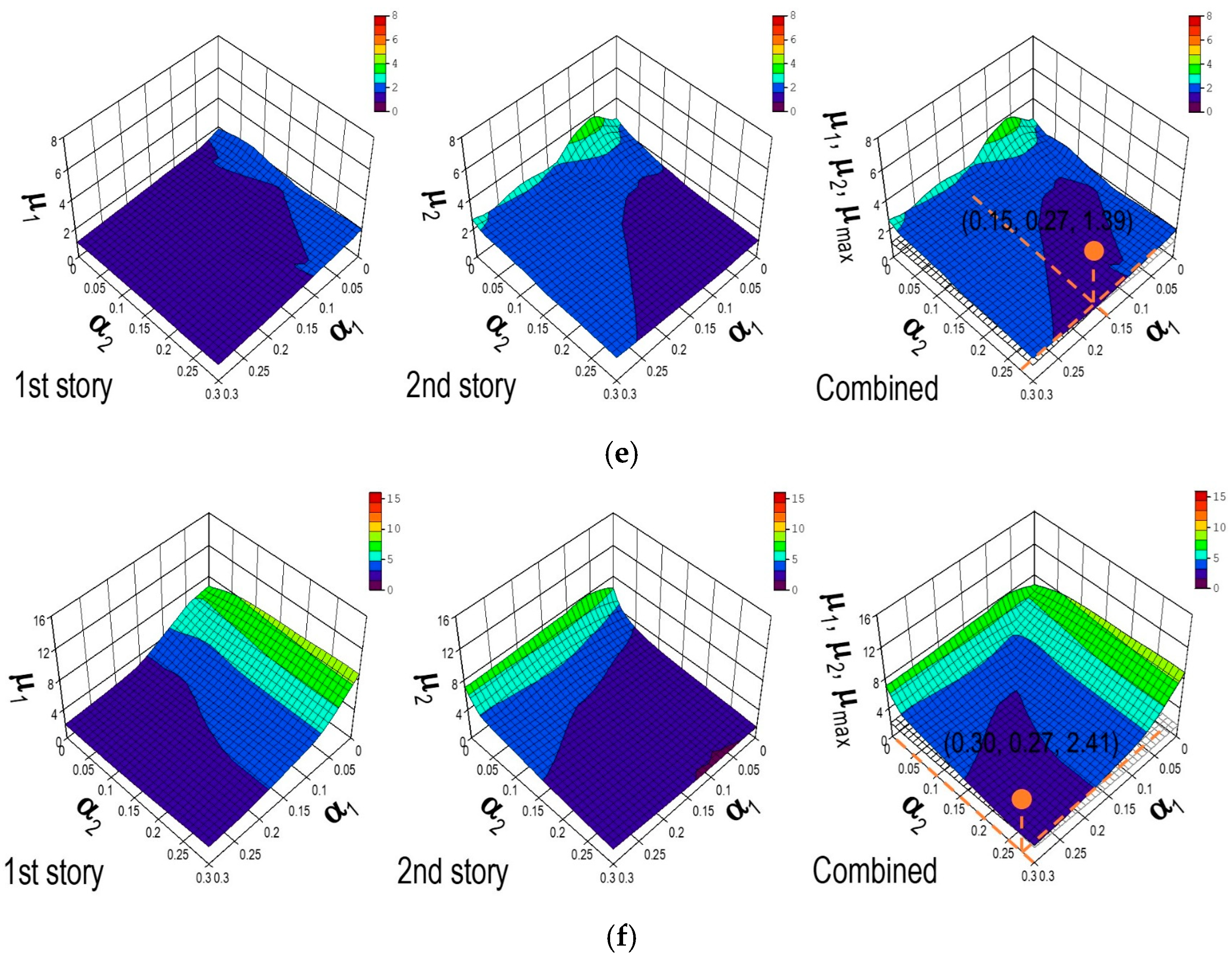
As shown in the later-stage results, Figure 8 vividly illustrates the trade-off relationship between the stiffness ratio (${\alpha }_i$) and the ductility factor (m_i = maximum story drift of ith story/${\delta }_{y_i}$) for the first and second stories’ round-robin response surface. The stiffness ratio is defined as the ratio of the LDEBs to the frame’s stiffness (${\alpha }_i=K_{b_i}/(K_{b_i}+K_{f_i}$). The ductility factor is a measure of how much the brace can deform before failure. These figures also depict the combined results of the first and second stories. The global optimum point on the graph where the stiffness ratio was minimized corresponds to the PSO results in Table 5, Table 6 and Table 7.

This study clearly states that the optimal stiffness ratio for LDEBs depends on several factors, including the following:

• The earthquake intensity. Different earthquake intensities require different stiffness distributions to optimize the response.
• The natural periods of the structure. The natural periods of the structure influence how it interacts with earthquake forces, and the optimal stiffness ratio should account for these periods.
• Ground motion characteristics. The specific characteristics of the ground motion (e.g., frequency content) can also impact the optimal stiffness ratio.

Therefore, it is impossible to provide a single “best” stiffness ratio for all situations. The optimal value will vary, depending on the specific scenario and design requirements. This study presents optimization methods such as PSO and round-robin analysis to help determine the optimal stiffness ratio for a particular case.

10.1. Quantitative Comparative Analysis

While Table 5, Table 6 and Table 7 and the later–stage results in Figure 8 provide descriptive insights into the optimized stiffness ratios and ductility factors under various seismic intensities, a quantitative comparative analysis further clarifies the effectiveness of the optimization framework.

Table 8. Percentage reduction in maximum story drift after optimization.

Seismic Input	Unbraced Drift (cm)	Optimized Drift (cm)	Reduction (%)
Ohta NS (50 kine)	9.99	5.90	41.00%
Ohta NS (90 kine)	12.36	10.52	15.00%
BCJ-L1 (50 kine)	9.01	3.90	57.00%
BCJ-L1 (90 kine)	17.01	6.08	64.25%
Wakuya NS (50 kine)	5.35	2.78	48.00%
Wakuya NS (90 kine)	13.17	4.82	63.50%

summarizes the percentage reduction in maximum story drift achieved using PSO optimization compared with the unbraced frames (i.e., without LDEBs).

The formula to compute the percentage reduction in maximum story drift is

$$\mathrm{Reduction}\hspace{0.17em}\hspace{0.17em}(\%)={\displaystyle \frac{\mathrm{Unbraced}\hspace{0.17em}\mathrm{Drift}\hspace{0.17em}-\hspace{0.17em}\mathrm{Optimized}\hspace{0.17em}\mathrm{Drift}}{\mathrm{Unbraced}\hspace{0.17em}\hspace{0.17em}\mathrm{Drift}}}\hspace{0.17em}\hspace{0.17em}\times \hspace{0.17em}\hspace{0.17em}100$$

(9)

These findings show that optimized LDEB designs significantly enhance structural properties. Reductions in maximum story drift between 15% and more than 64%, depending on ground motion features and intensity. The maximum percentages of the reductions were found under the high-intensity inputs, which shows the superiority of the developed LDEB system under severe seismic actions.

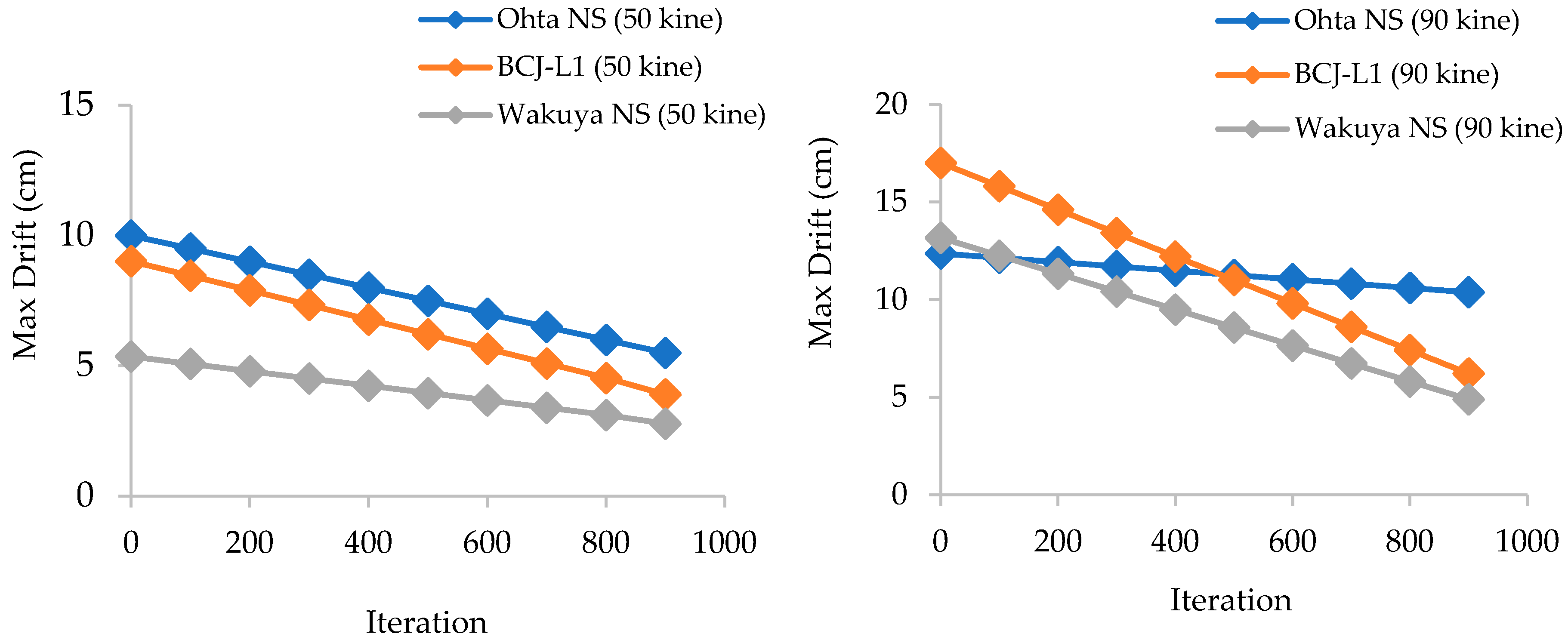
10.2. PSO Convergence Behavior

The convergence behavior of the PSO algorithm was monitored for all seismic input cases to assess its computational efficiency. The convergence histories for all the earthquake records at both 50-kine and 90-kine intensity levels, which are part of the later stage results, are shown in Figure 10.

In most scenarios, PSO achieved stable convergence within approximately 800 iterations, significantly below the maximum allowed 3000 iterations. The smooth and consistent decline in the objective function across all cases indicated stable search behavior, the efficient exploration of the solution space, and the reliable identification of global optimal stiffness distributions.

The PSO convergence behavior for all the seismic inputs is presented. The left subfigure shows the convergence for Ohta NS, BCJ-L1, and Wakuya NS under a 50-kine seismic intensity. The right subfigure shows the convergence for the same earthquake records under a 90-kine intensity. PSO achieved convergence within 800–900 iterations across all cases, confirming the robustness and stability of the optimization framework.

10.3. Relationship Between Stiffness and Ductility

Figure 7 visualizes the relationship between the stiffness ratios and ductility factors. As the LDEB stiffness ratios increased, the ductility factors decreased, reflecting reduced deformation demands. However, excessive stiffness can elevate higher mode participation, potentially introducing detrimental dynamic effects. Therefore, the optimal solution balances sufficient stiffness to suppress drift while maintaining flexibility to avoid adverse higher-mode amplification.

11. Numerical Results Determined by Round-Robin Analysis

This study underscores the suitability of steel construction in earthquake-prone regions and emphasizes the critical concept of seismic resilience. Specifically, this research introduced LDEBs to enhance seismic performance in structural design. The investigation carried out as part of this study focused on steel buildings incorporating LDEBs, which were represented as 2-DOF systems (Figure 1).

Figure 2 and Table 2 present the natural periods of the two-story model. These periods could have been used to inform the initial stiffness ratios for the PSO and round-robin analyses. For instance, knowing the dominant vibration modes (shapes) and corresponding periods could help tailor the stiffness distribution to better counteract specific earthquake frequencies.

Figure 3 showcases a three-velocity response spectrum, revealing how our structure responded to different earthquake scenarios. Under the Ohta NS wave, the first mode swayed a significant 56 kine, while the second mode followed closely, at 100 kine. The BCJ-L1 wave elicited a more subdued response, with 70 kine in the first mode and 28 kine in the second. The Wakuya NS wave was the most potent, sending the first mode rocketing to 117 kine, while the second mode peaked at 58 kine. These insights, along with additional velocity response spectra presented in Figure 3 for various seismic events, could have been leveraged in two key ways: firstly, by strategically choosing scaled velocity levels (50 and 90 kine) for optimization and, secondly, by guiding the initial placement of the stiffness ratios within the optimization algorithms’ search space. This would have ensured that our structure was adequately prepared to handle diverse tremors.

Figure 8 demonstrates the relationship between the maximum story drift and story stiffness ratio determined by the round-robin analysis. The orange data points on the graphs represent the results obtained from the PSO approach, specifically highlighting the minimum solutions achieved through PSO. These figures consistently show valley-shaped response surfaces, illustrating the model’s behavior during significant seismic events. The valley-shaped surfaces consisted of the first- and second-story response surfaces combined. Moreover, the first-story response became the same as the second-story response, and the two stories gave a smaller response locally on the valley lines. Consequently, the PSO solutions were located on the valley lines in almost all cases. The findings from both the PSO and the round-robin experiments validate the PSO minimum solution as the global optimum of the round-robin response surface. Ultimately, these insights highlight the impact of inherent frequency alterations on stiffness ratios, resulting in the structure’s enhanced strength, durability, and usability during moderate seismic events and severe earthquakes.

Figure 8c–f for BCJ-L1 and Wakuya NS wave shows that ${\mu }_1$ decreased as ${\alpha }_1$ increased, and ${\mu }_2$ decreased as ${\alpha }_2$ increased. Consequently, this result formed a valley shape centered on the combined response surface. Meanwhile, the results are difficult to understand in the case of the Ohta wave. Figure 8a,b demonstrates that ${\mu }_2$ significantly increased as ${\alpha }_1$ increased in the small ${\alpha }_2$ region. This difficult-to-understand result shifted the valley shape rightward on the combined response surface. The reason for this result is that increasing ${\alpha }_1$ led to increasing the second mode response. We can observe the first peak at 0.23 s of the natural period on the response spectrum for the Ohta wave, as shown in Figure 3.

Table 2 shows that the natural periods of both the first and second modes decreased as the LDEBs’ stiffness ratio increased. This means that the structures became stiffer as the LDEBs became stiffer. This is because the LDEBs added stiffness to the structure, which reduced the overall stiffness of the system. As a result, the structures vibrated at lower frequencies (longer periods).

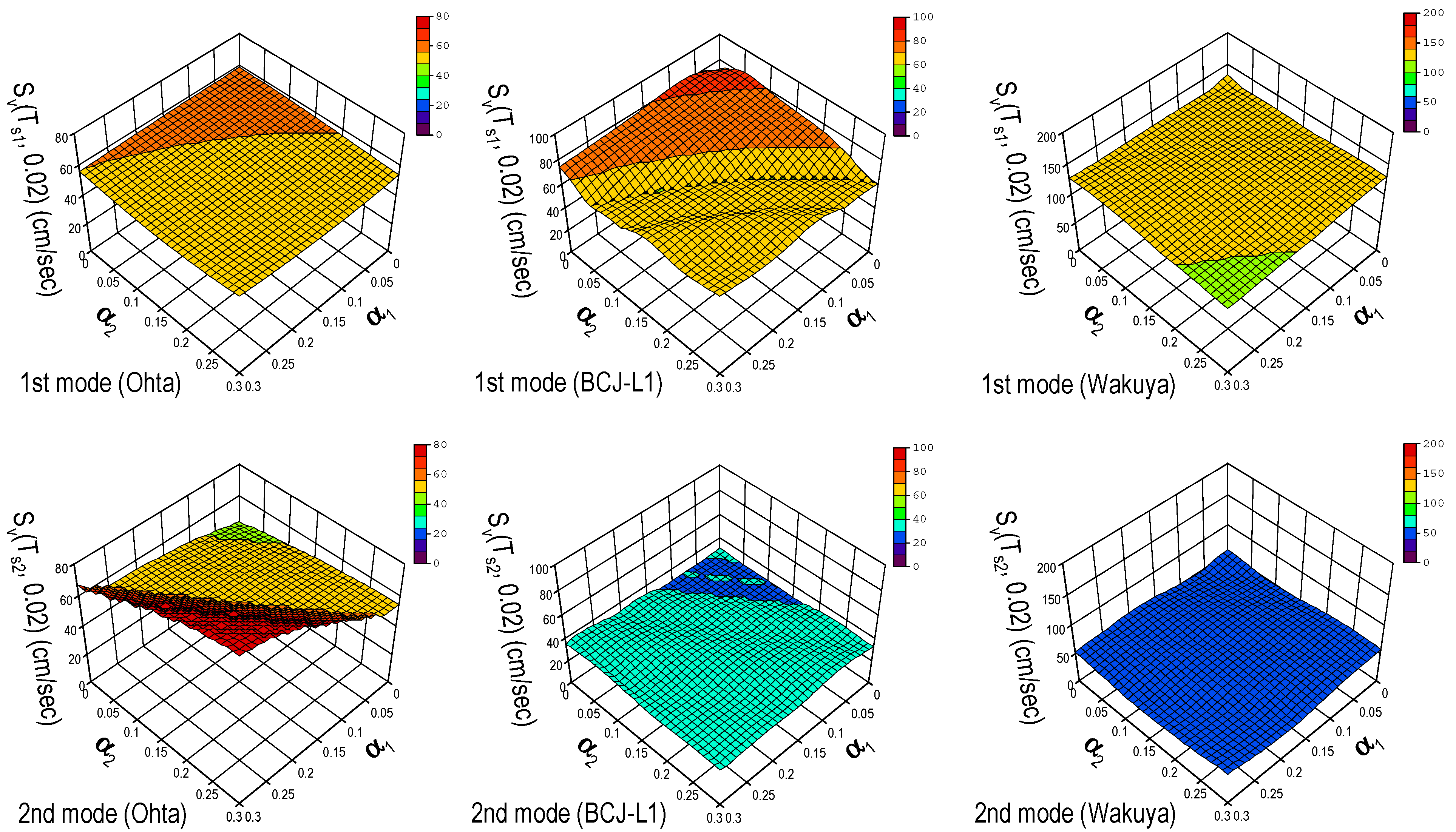
Figure 9 shows the changes in the mode shapes due to the varying stiffness ratio. The mode shapes are plotted as the relative displacement of each floor, with the first floor was fixed at one. As the stiffness ratio increased, the mode shapes became more concentrated in the lower floors. This means that the upper floors vibrated less compared with the lower floors. This is because the LDEBs were on the lower floors, and they added more stiffness to these floors.

Figure 10 shows that the spectral velocity values at both the first and second modes decreased as the LDEBs’ stiffness ratio increased, except for the second mode of Ohta. This means that the structures became stiffer as the LDEBs became stiffer. This is consistent with the observations made in Table 2 and Figure 9, which are illustrated in Figure 10 and discussed in a later section.

This study successfully demonstrated the effectiveness of LDEBs in enhancing the seismic resilience of steel structures. LDEBs, despite seeming to decrease stiffness, led to improved strength, durability, and reduced story drift. Optimizing the LDEBs’ placement and stiffness ratios proved crucial, suggesting potential for wider use in earthquake-prone regions.

12. Limitations

In this paper, response surfaces were visualized for just two-design-variable models (SDOF). In cases with more than three design variables, we can visualize response surfaces on any two-design-variable axes around a PSO optimum solution.

This study adopted a damping model that assumed proportionality to the total stiffness, which included contributions from both the main frame and the LDEBs. Although this approach enables computational efficiency and is widely used in seismic analysis, it cannot fully capture the complex damping behaviors for geometrically nonlinear components. LDEBs may introduce additional damping effects related to their large deformation capacity, restoring forces, and interaction with the main structural frame. Therefore, the current assumption may lead to some simplification of the dynamic response, particularly under strong seismic excitation. Future studies are encouraged to explore more detailed damping models that incorporate these nonlinear effects for a more comprehensive evaluation of LDEBs’ performance.

13. Conclusions

This study showed that LDEBs can effectively improve the seismic performance of steel structures. Using LDEBs can lead to increased strength, durability, and reduced story drift. Optimizing LDEBs’ placement and stiffness ratios proved crucial, suggesting potential for wider use in earthquake-prone regions.

Below are some of the key findings of this study:

• Optimized LDEB stiffness distributions significantly reduced maximum story drifts and ductility demands across different seismic inputs, achieving drift reductions ranging from 15% to over 64%, depending on the earthquake characteristics.
• The optimal stiffness distribution of LDEBs depends on the earthquake intensity, the natural periods of the structure, and the ground motion frequency content. LDEBs dynamically shift natural periods away from resonance regions, suppressing the amplification of the seismic response and minimizing damage.
• PSO is an effective method for finding the optimal stiffness distribution of LDEBs.
• Round-robin analysis can be used to validate PSO results and provide additional insights into the behavior of the structure.

Overall, this study provides valuable insights for designers who are considering using LDEBs to improve the seismic performance of steel structures. By optimizing the placement and stiffness of LDEBs, designers can create structures that exhibit favorable modal behavior, reduce both first- and higher-mode amplifications, and enhance seismic resilience across a wide range of earthquake intensities. In particular, by integrating PSO with round-robin analysis, this study provides a more comprehensive optimization and validation framework, which allows designers to capture global optima while simultaneously visualizing the sensitivity of structural responses across a broad range of stiffness configurations and seismic intensities. This dual approach advances current optimization practices for LDEBs beyond conventional methods.

Furthermore, the PSO-based optimization framework developed in this study holds significant potential for practical engineering applications. In early-stage design, it enables structural engineers to identify optimal LDEB stiffness distributions that shift structural periods away from resonance zones and minimize inter-story drift, leading to enhanced seismic resilience while ensuring material and cost efficiency. In retrofit scenarios, this approach can guide the selective implementation of LDEBs in existing structures, improving seismic performance without requiring major structural alterations. The integrated PSO equipment with round-robin validation guarantees both the overall optimization and the seismic diversity and robustness of these optimum design solutions so engineers can make performance-based decisions for buildings constructed in seismic zones.