
A CCP-Based Decentralized Optimization Approach for Electricity–Heat Integrated Energy Systems with Buildings

Abstract
1. Introduction
2. Optimization Model of EH-IESs, Considering Building Thermal Inertia
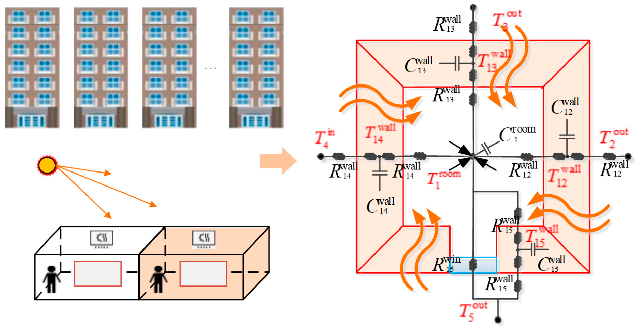
2.1. Detailed Thermal Dynamic Model of Buildings
2.2. Power Flow Model of the ES
2.3. Operation Model of TS
2.3.1. The Model of CHP Units
2.3.2. The Heating Network Model
3. A CCP-Based Optimization Approach for EH-IESs with Buildings
3.1. Objective Function
3.2. Deterministic Transformation of CCP
4. An ADMM-Based Decentralized Solution Method for EH-IESs with Buildings
- The subproblem for ES is as follows:where is the vector composed of Lagrange multipliers on the ES side; is the vector composed of coupled variables; is the vector composed of global variables; is the iteration step size; and is the connecting line that couples two subsystems.
- The subproblem for TS is as follows:where is the vector composed of Lagrange multipliers on the TS side; is the vector composed of coupled variables on the TS side.
5. Case Studies
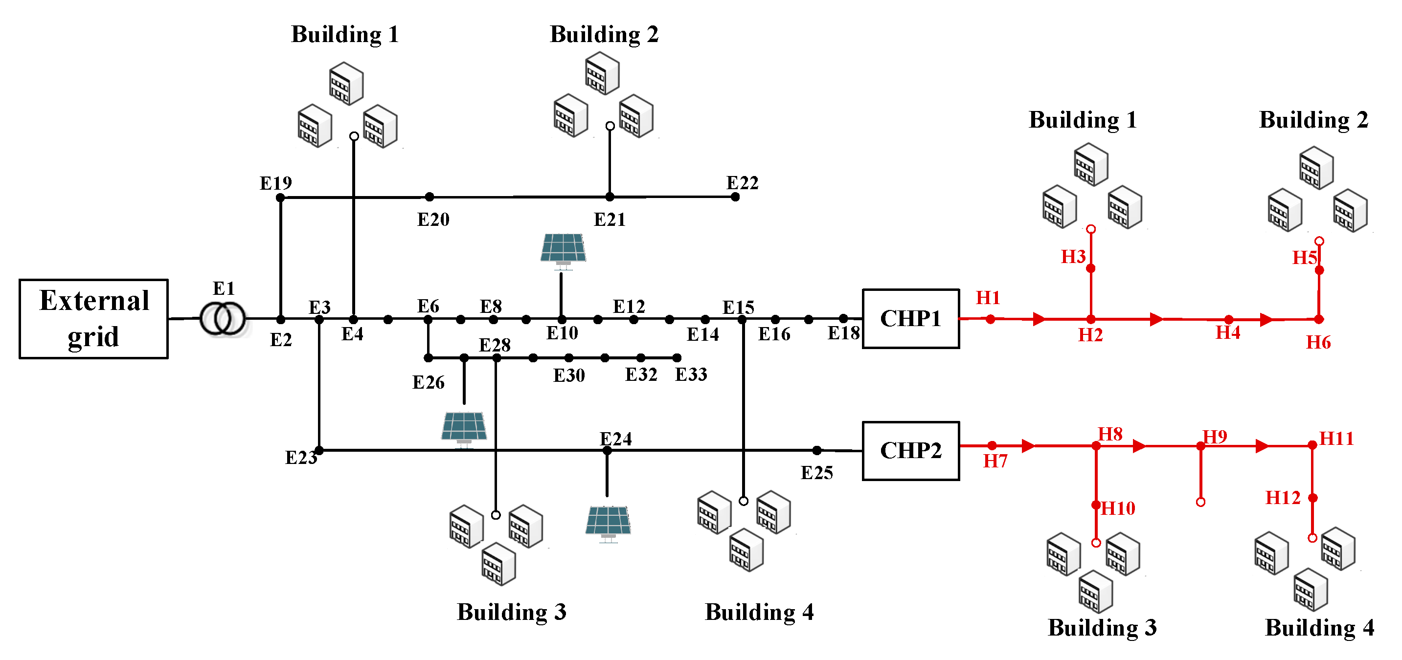
5.1. Case Data
5.2. Case Results and Analysis
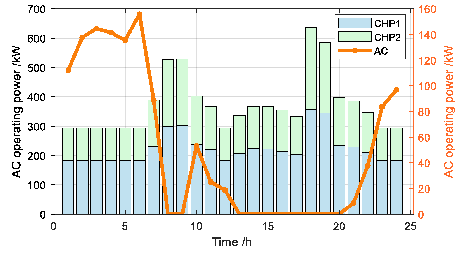
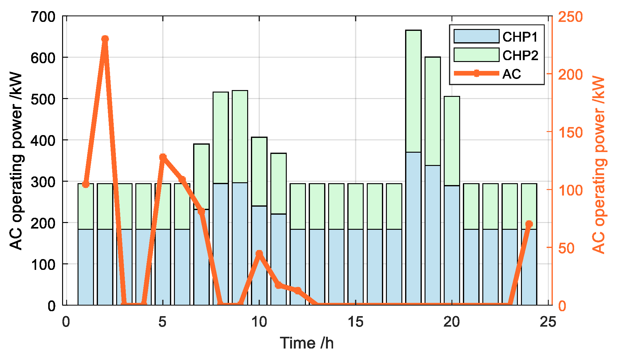
5.2.1. Impact Analysis of Heating Systems and User Comfort Levels on EH-IES Operation
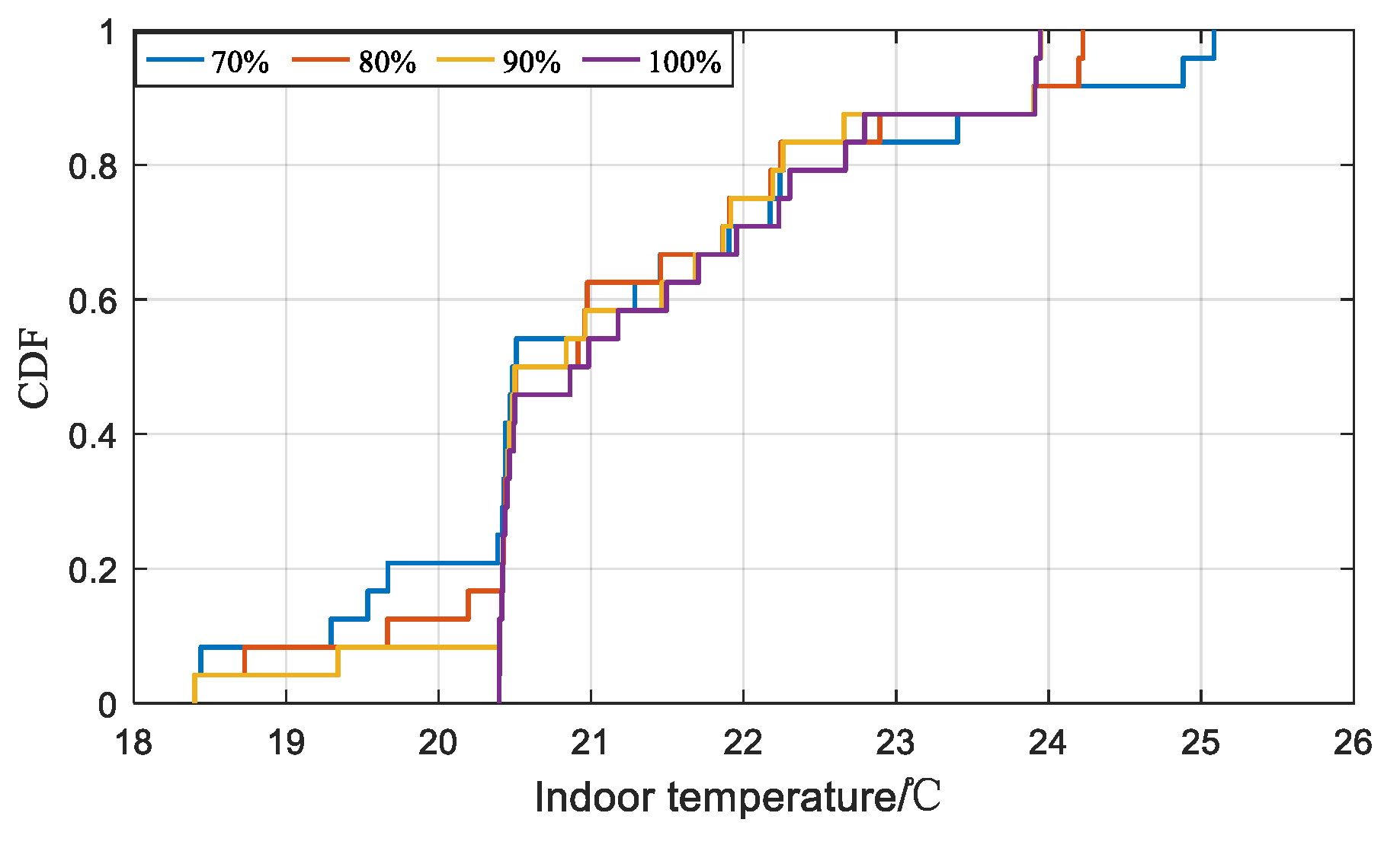
5.2.2. Analysis of EH-IES Optimization Results Based on CCP
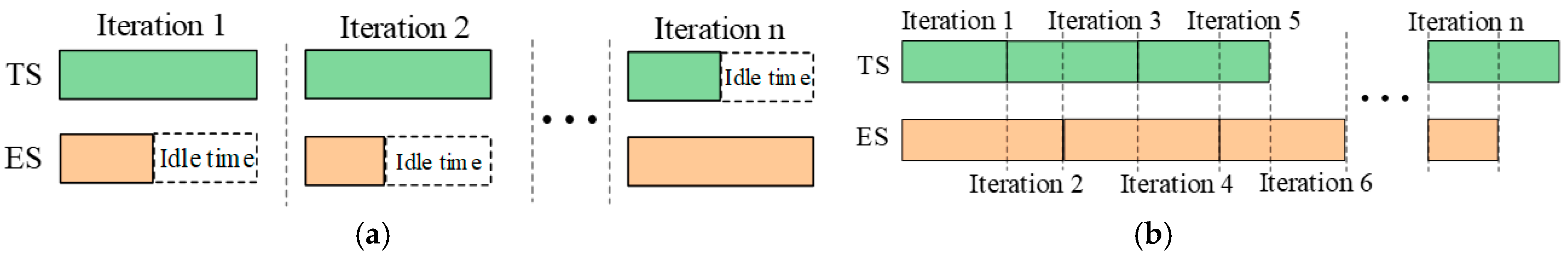
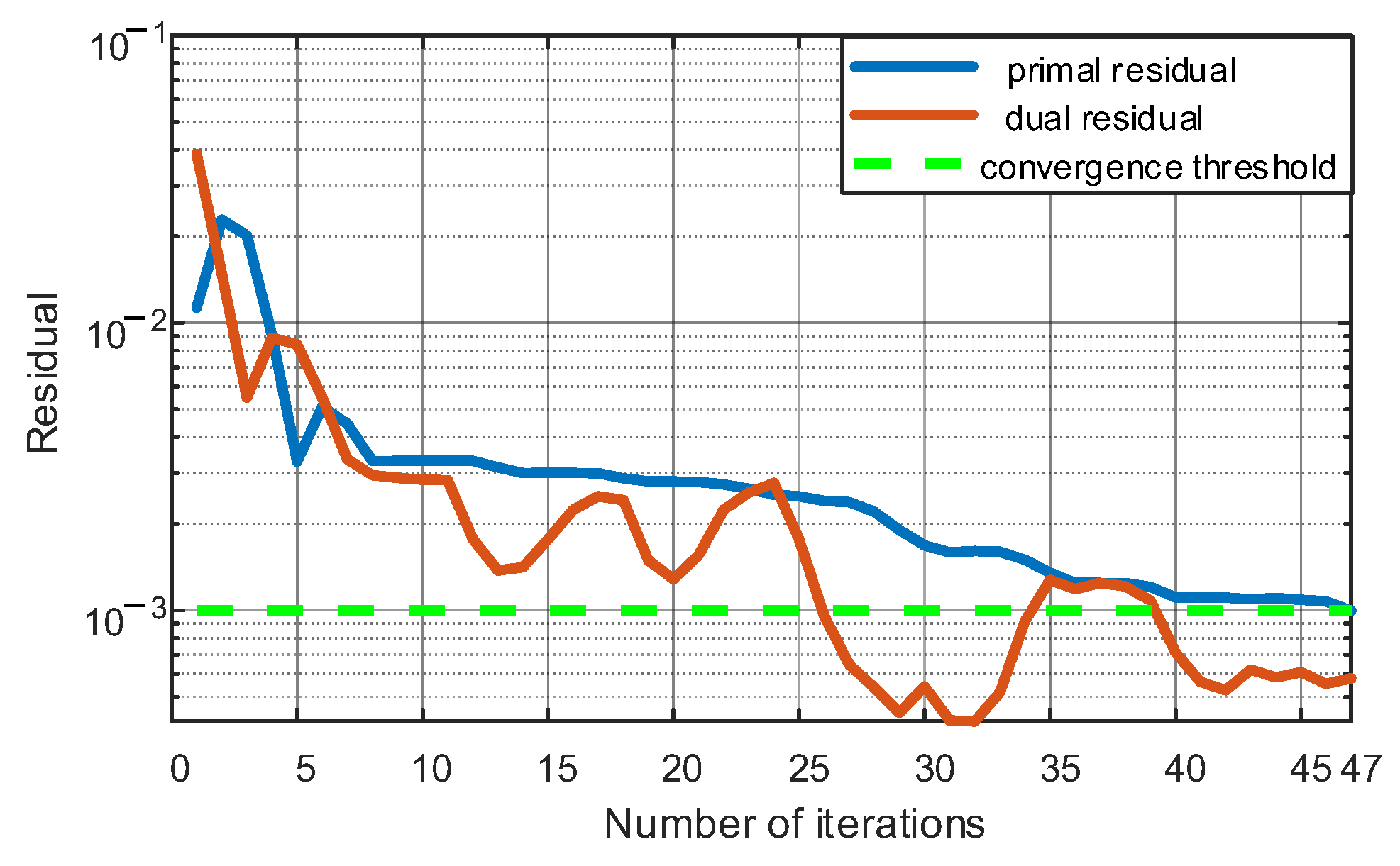
5.2.3. Convergence and Optimality Analysis of the A-AD-ADMM Algorithm
6. Conclusions
Author Contributions
Funding
Data Availability Statement
Conflicts of Interest
References
- Ding, C.; Zhang, X.; Liang, G.; Feng, J. Optimizing exergy efficiency in integrated energy system: A planning study based on industrial waste heat recovery. IEEE Access 2024, 12, 148074–148089. [Google Scholar] [CrossRef]
- Wang, Y.; Hu, J.; Liu, N. Energy management in integrated energy system using energy–carbon integrated pricing method. IEEE Trans. Sustain. Energy 2023, 14, 1992–2005. [Google Scholar] [CrossRef]
- Zhang, Y.; Hao, J.; Ge, Z.; Zhang, F.; Du, X. Optimal clean heating mode of the integrated electricity and heat energy system considering the comprehensive energy-carbon price. Energy 2021, 231, 120919. [Google Scholar] [CrossRef]
- Wang, X.; Li, Z.; Shahidehpour, M.; Jiang, C. Robust Line Hardening Strategies for Improving the Resilience of Distribution Systems with Variable Renewable Resources. IEEE Trans. Sustain. Energy 2019, 10, 386–395. [Google Scholar] [CrossRef]
- Yan, Q.; Zhang, G.; Zhang, Y.; Yu, H. Coordinated scheduling optimization of building integrated energy system with flexible load. Energy Rep. 2024, 12, 3422–3436. [Google Scholar] [CrossRef]
- Liu, X.; Hou, M.; Sun, S.; Wang, J.; Sun, Q.; Dong, C. Multi-time scale optimal scheduling of integrated electricity and district heating systems considering thermal comfort of users: An enhanced-interval optimization method. Energy 2022, 254, 124311. [Google Scholar] [CrossRef]
- Cheng, X.; Liu, L.; Huang, W.; Sun, Y.; Sun, K.; Zhang, X.; Ren, A. Optimal dispatch of the electricity-heat integrated energy system under epistemic uncertainty of thermal-inertia based flexible demand response. In Proceedings of the 2023 IEEE 7th Conference on Energy Internet and Energy System Integration, Hangzhou, China, 15–18 December 2023; pp. 819–823. [Google Scholar]
- Wang, K.; Xue, Y.; Zhou, Y.; Li, Z.; Chang, X.; Sun, H. Distributed coordinated reconfiguration with soft open points for resilience-oriented restoration in integrated electric and heating systems. Appl. Energy 2024, 365, 123207. [Google Scholar] [CrossRef]
- Huang, S.; Wu, Q.; Guo, Y.; Chen, X.; Zhou, B.; Li, C. Distributed voltage control based on ADMM for large-scale wind farm cluster connected to VSC-HVDC. IEEE Trans. Sustain. Energy 2019, 11, 584–594. [Google Scholar] [CrossRef]
- Jiang, L.; Bie, Z.; Long, T.; Xie, H.; Xiao, Y. Distributed energy management of integrated electricity-thermal systems for high-speed railway traction grids and stations. CSEE J. Power Energy Syst. 2020, 7, 541–554. [Google Scholar]
- Wu, Y.; Wang, C.; Wang, Y. Cooperative game optimization scheduling of multi-region integrated energy system based on ADMM algorithm. Energy 2024, 302, 131728. [Google Scholar] [CrossRef]
- Ding, B.; Li, Z.; Li, Z.; Xue, Y.; Chang, X.; Su, J.; Jin, X.; Sun, H. A CCP-based distributed cooperative operation strategy for multi-agent energy systems integrated with wind, solar, and buildings. Appl. Energy 2024, 365, 123275. [Google Scholar] [CrossRef]
- Zhou, J.; Liu, W.; Chen, X.; Sun, M.; Mei, C.; He, S.; Gao, H.; Liu, J. A distributionally robust chance constrained planning method for integrated energy systems. In Proceedings of the 2019 IEEE PES Asia-Pacific Power and Energy Engineering Conference, Macao, China, 1–4 December 2019; pp. 1–5. [Google Scholar]
- An, H.; Lin, W.; Jin, X.; Zhou, Q.; Cen, B. Stochastic multi-objective scheduling approach for integrated community energy system. In Proceedings of the 2018 IEEE International Conference on Energy Internet, Beijing, China, 21–25 May 2018; pp. 321–325. [Google Scholar]
- Jin, X.; Wu, Q.; Jia, H.; Hatziargyriou, N.D. Optimal integration of building heating loads in integrated heating/electricity community energy systems: A bi-level MPC approach. IEEE Trans. Sustain. Energy 2021, 12, 1741–1754. [Google Scholar] [CrossRef]
- Ding, B.; Li, Z.; Li, Z.; Xue, Y.; Chang, X.; Su, J.; Sun, H. Cooperative Operation for Multiagent Energy Systems Integrated With Wind, Hydrogen, and Buildings: An Asymmetric Nash Bargaining Approach. IEEE Trans. Ind. Inform. 2025; early access. [Google Scholar]
- Zhang, R.; Chu, X.; Zhang, W.; Liu, Y. Active participation of air conditioners in power system frequency control considering users’ thermal comfort. Energies 2015, 8, 10818–10841. [Google Scholar] [CrossRef]
- Standard 55-2004; Thermal Environmental Conditions for Human Occupancy. ASHRAE Inc.: Atlanta, GA, USA, 2004.
- Zhang, H.; Li, Z.; Xue, Y.; Chang, X.; Su, J.; Wang, P.; Guo, Q.; Sun, H. A stochastic bi-level optimal allocation approach of intelligent buildings considering energy storage sharing services. IEEE Trans. Consum. Electron. 2024, 70, 5142–5153. [Google Scholar] [CrossRef]
- Wang, X.; Shahidehpour, M.; Jiang, C.; Li, Z. Coordinated Planning Strategy for Electric Vehicle Charging Stations and Coupled Traffic Electric Networks. IEEE Trans. Power Syst. 2019, 34, 268–279. [Google Scholar] [CrossRef]
- Wang, K.; Xue, Y.; Guo, Q.; Shahidehpour, M.; Zhou, Q.; Wang, B.; Sun, H. A coordinated reconfiguration strategy for multi-stage resilience enhancement in integrated power distribution and heating networks. IEEE Trans. Smart Grid 2022, 14, 2709–2722. [Google Scholar] [CrossRef]
- Cui, X.; Liang, L.; Liu, W.; Yin, W.; Liu, J.; Hou, Y. Modeling EV dynamic wireless charging loads and constructing risk constrained operating strategy for associated distribution systems. Appl. Energy 2025, 378, 124735. [Google Scholar] [CrossRef]
- Xue, Y.; Li, Z.; Lin, C.; Guo, Q.; Sun, H. Coordinated dispatch of integrated electric and district heating systems using heterogeneous decomposition. IEEE Trans. Sustain. Energy 2019, 11, 1495–1507. [Google Scholar] [CrossRef]
- Du, Y.; Xue, Y.; Wu, W.; Shahidehpour, M.; Shen, X.; Wang, B.; Sun, H. Coordinated Planning of Integrated Electric and Heating System Considering the Optimal Reconfiguration of District Heating Network. IEEE Trans. Power Syst. 2024, 1, 794–808. [Google Scholar] [CrossRef]
- Fang, X.; Shen, Y.; Zhou, J.; Pantelous, A.A.; Zhao, M. QFD-based product design for multisegment markets: A fuzzy chance-constrained programming approach. IEEE Trans. Eng. Manag. 2020, 69, 2296–2310. [Google Scholar] [CrossRef]
- Li, X.; Li, W.; Zhang, R.; Jiang, T.; Chen, H.; Li, G. Collaborative scheduling and flexibility assessment of integrated electricity and district heating systems utilizing thermal inertia of district heating network and aggregated buildings. Appl. Energy 2020, 258, 114021. [Google Scholar] [CrossRef]
- Chen, H.; Zhang, Y.; Zhang, R.; Lin, C.; Jiang, T.; Li, X. Privacy-preserving distributed optimal scheduling of regional integrated energy system considering different heating modes of buildings. Energy Convers. Manag. 2021, 237, 114096. [Google Scholar] [CrossRef]
- Li, Z.; Su, S.; Jin, X.; Xia, M.; Chen, Q.; Yamashita, K. Stochastic and distributed optimal energy management of active distribution networks within integrated office buildings. CSEE J. Power Energy Syst. 2022, 10, 504–517. [Google Scholar]
- Zhai, X.; Li, Z.; Li, Z.; Xue, Y.; Chang, X.; Su, J.; Jin, X.; Wang, P.; Sun, H. Risk-averse energy management for integrated electricity and heat systems considering building heating vertical imbalance: An asynchronous decentralized approach. Appl. Energy 2025, 383, 125271. [Google Scholar] [CrossRef]
- Li, Z.; Su, S.; Jin, X.; Chen, H. Distributed energy management for active distribution network considering aggregated office buildings. Renew. Energy 2021, 180, 1073–1087. [Google Scholar] [CrossRef]


| Confidence Level | Total Operating Cost /USD |
|---|---|
| 100% | 5002.9 |
| 90% | 4959.6 |
| 80% | 4878.2 |
| 70% | 4756.24 |
| Algorithm | Iterations | Solution Time/s |
|---|---|---|
| Traditional ADMM | 35 | 743.62 |
| SP-ADMM | 35 | 269.64 |
| AD-ADMM | 63 | 133.55 |
| A-AD-ADMM | 47 | 89.34 |
Disclaimer/Publisher’s Note: The statements, opinions and data contained in all publications are solely those of the individual author(s) and contributor(s) and not of MDPI and/or the editor(s). MDPI and/or the editor(s) disclaim responsibility for any injury to people or property resulting from any ideas, methods, instructions or products referred to in the content. |
© 2025 by the authors. Licensee MDPI, Basel, Switzerland. This article is an open access article distributed under the terms and conditions of the Creative Commons Attribution (CC BY) license (https://creativecommons.org/licenses/by/4.0/).
Share and Cite
Zhai, X.; Qin, X.; Zhang, J.; Liu, X.; Bai, X.; Zhang, S.; Ma, Z.; Li, Z. A CCP-Based Decentralized Optimization Approach for Electricity–Heat Integrated Energy Systems with Buildings. Buildings 2025, 15, 2294. https://doi.org/10.3390/buildings15132294
Zhai X, Qin X, Zhang J, Liu X, Bai X, Zhang S, Ma Z, Li Z. A CCP-Based Decentralized Optimization Approach for Electricity–Heat Integrated Energy Systems with Buildings. Buildings. 2025; 15(13):2294. https://doi.org/10.3390/buildings15132294
Chicago/Turabian StyleZhai, Xiangyu, Xuexue Qin, Jiahui Zhang, Xiaoyang Liu, Xiang Bai, Song Zhang, Zhenfei Ma, and Zening Li. 2025. "A CCP-Based Decentralized Optimization Approach for Electricity–Heat Integrated Energy Systems with Buildings" Buildings 15, no. 13: 2294. https://doi.org/10.3390/buildings15132294
APA StyleZhai, X., Qin, X., Zhang, J., Liu, X., Bai, X., Zhang, S., Ma, Z., & Li, Z. (2025). A CCP-Based Decentralized Optimization Approach for Electricity–Heat Integrated Energy Systems with Buildings. Buildings, 15(13), 2294. https://doi.org/10.3390/buildings15132294