Equivalent Input Energy Velocity of Elastoplastic SDOF Systems with Specific Strength

Abstract

This paper presents the results of statistical analyses carried out for the input energy velocity (equivalent velocity to be used for the determination of the input energy) of equivalent single-degree-of-freedom systems with definite strength. An earthquake ground motion database, which includes 268 far-field records and two horizontal components from 134 recording stations located on firm sites, is employed for nonlinear time–history analysis. The probabilistic distribution of the input energy velocity is investigated for the candidate distribution models through a chi-square test, and the lognormal distribution was found as the most representative distribution model. Furthermore, the data used for analysis are classified with respect to the considered strength reduction factors of SDOF systems as a structural parameter and the effective duration of the considered strong ground motions as a ground motion parameter. The effect of those parameters on input energy velocity is investigated by using probabilistic techniques such as t-tests and ANOVAs. It is concluded that the strength reduction factor influences the input energy velocity along the particular period ranges of SDOF systems. Furthermore, the effective duration of the ground motion is another effective parameter on input energy velocity for almost all the considered period ranges. An equation is proposed for the determination of input energy velocity in terms of the aforementioned parameters.

1. Introduction

Structures subjected to earthquake forces, exceeding the design strength specified in seismic codes, may exhibit inelastic behavior during their seismic response, leading to structural damage. Controlling this possible damage is a primary objective in modern seismic design practice. Furthermore, assessing the seismic performance of existing structures to accurately predict potential structural and non-structural damage has always been another major concern of structural engineering. Thus, performance-based design methodologies have been adopted by all seismic design codes. Those methods mainly focus on the estimation of the maximum displacement demand imposed by a ground motion. However, several researchers have emphasized that the reason of structural damage is not solely caused by the peak deformation experienced by the system but also by the hysteretic energy dissipated during a seismic event [1,2,3,4,5,6,7,8,9,10,11]. The concept of energy-based design was first proposed by G. W. Housner [12], who demonstrated that a structure dissipates energy through damping and nonlinear behavior, while the remaining energy is stored as kinetic and elastic strain energy. There are several studies in the literature which investigated the input energy and the hysteretic energy of structures [13,14,15,16,17,18,19,20,21].

Mezgebo and Lui [13] developed input energy and hysteretic energy spectra which take the soil site, hysteretic model, and ductility into consideration for far-fault earthquakes. Mezgebo and Lui [14] also proposed a method for applying input and hysteretic energy spectra, originally developed for single-degree-of-freedom systems, to multi-degree-of-freedom steel moment-resisting frames. Homaei [15] investigated the effect of soil–structure interaction on hysteretic energy demands through nonlinear time–history analysis of single-degree-of-freedom systems and concluded that soil–structure interaction significantly decreases the hysteretic energy demand of systems whose period is relatively shorter. Hasanoğlu et al. [16] investigated constant ductility input and hysteretic energy transferred to different single-degree-of-freedom systems by near-field ground motions. Empirical correlations between energy-based intensity measures and conventional spectrum-based, peak amplitude-based, and cumulative-based measures were investigated based on time–history analyses. Furthermore, predictive models between energy parameters and spectral acceleration were suggested across different ductility levels.

In this paper, results of the statistical analysis carried out for the input energy velocity to be used for the determination of the input energy, are presented for elastoplastic SDOF systems with definite strength. Effect of the hysteresis type on the seismic performance of structural systems have been explored in some previous studies. Rahnama and Krawinkler [22], Foutch and Shi [23], Huang and Foutch [24] have observed that there is no clear correlation between the hysteresis type and the ductility demand. On the other hand, Ibarra et al. [25] have demonstrated that deterioration becomes effective when the system approaches its global collapse state. Furthermore, Dindar et al. [17] observed that hysteretic energy demand spectra of elastoplastic model is conservative comparing that of other models which included different degrading types. Thus, elastoplastic SDOF systems with 5% critical damping have been considered within the scope of this study, since those systems can be defined with a few parameters that represent the structural stiffness and strength. A correlation matrix was generated by considering a number of parameters, which represent the different characteristics of structure and ground motion to investigate the correlation between those considered parameters and the input energy velocity. It is observed that strength reduction factor (R_y) influences the input energy velocity along the particular period ranges, while the effective duration of the ground motion (t_d) is another effective parameter on input energy velocity for almost all considered period ranges. The analyzed data was classified with respect to both considered strength reduction factors of SDOF systems and the effective duration of considered ground motions. The effect of those parameters on input energy velocity was investigated by using probabilistic techniques such as t-tests and ANOVAs. Finally, an equation is proposed for the input energy velocity in terms of strength reduction factor and effective duration of ground motion.

2. Materials and Methods

2.1. Seismic Energy Demand

The equation of motion for an inelastic damped SDOF system, whose elastoplastic force-displacement relationship is shown in Figure 1, subjected to a ground motion can be written as:

$$m\ddot{u}\left(t\right)+c\dot{u}\left(t\right)+f_s\left(u,\dot{u}\right)=-m{\ddot{u}}_g\left(t\right)$$

(1)

where m is the mass, c is the viscous damping coefficient, f_s is the restoring force, u is the relative displacement of the mass with respect to the ground. $\dot{u}$, $\ddot{u}$, ${\ddot{u}}_g$ are velocity, acceleration, and the ground motion acceleration, respectively. The energy balance equation can be written as follows, using the transformation of $du=\dot{u}\left(t\right)dt$

$$\underset{0}{\overset{u}{\int }}m\ddot{u}\left(t\right)du+\underset{0}{\overset{u}{\int }}c\dot{u}\left(t\right)du+\underset{0}{\overset{u}{\int }}{f}_s\left(u,\dot{u}\right)du=-\underset{0}{\overset{u}{\int }}m{\ddot{u}}_g\left(t\right)du$$

(2)

The first term and the right-hand side of Equation (2) represent relative kinetic energy (E_k) and relative input energy (E_i), as defined by Uang and Bertero [18]. The second term corresponds to viscous damping energy, which is dissipated through viscous damping, while the third term represents hysteretic energy, comprising irrecoverable energy and elastic strain energy. E_k vanishes at the end of vibration. A significant portion of the maximum input energy is stored as kinetic energy and elastic strain energy, neither of which contribute to the cumulative damage of the structure. Elastic strain energy results from the structure’s elastic deformation and reduces to zero when the vibration ends, meaning it does not cause permanent damage. The third term of Equation (2), known as hysteretic energy, is associated with the system’s inelastic deformation. As stated by Manfredi [7], the input energy at the end of the ground motion is more appropriate measure for cumulative damage assessment than the maximum input energy, since it includes all the inelastic cycles experienced by the structure. Thus, in this study, the relative input energy accumulated at the end of the ground motion is considered and hereinafter referred to as input energy. It is worth noting that absolute and relative input energies become equal at the end of the ground motion since the relative kinetic energy vanishes. Housner [12] proposed Equation (3) for the input energy per unit mass

$${\displaystyle \frac{E_i}{m}}={\displaystyle \frac{1}{2}}{\left(PSV\right)}^2$$

(3)

where PSV is pseudo-spectral velocity. Akiyama [2] (1985), considering the three ground motion records, stated that Equation (3) is also valid for nonlinear behavior and input energy velocity can be used instead of PSV for the determination of input energy, as follows

$${\displaystyle \frac{E_i}{m}}={\displaystyle \frac{1}{2}}{\left(V_E\right)}^2$$

(4)

Nakashima et al. [19] (1996) concluded that the input energy of a MDOF system can be estimated using the equivalent SDOF system. The estimation of seismic input energy of structures has also been the subject of several investigations [6,7,9,19,20]. All the aforementioned studies estimate the spectral input energy by means of the input energy velocity as given in Equation (5).

$$V_E=\sqrt{{\displaystyle \frac{{2E}_i}{m}}}$$

(5)

Dindar et al. have studied the input and hysteretic energy demand spectra [17]. More recently, Güllü et al. [21] made an experimental assessment and formulated a three-part mass-normalized relative input energy spectrum considering the soil type, ground motion parameters and structural parameters such as corner period, intensity, duration, spectral acceleration, velocity, structural period, and structural damping. Gholami et al. [26] published a state-of-the-art report on energy based seismic design methods. Another investigation on input energy has been performed by Zhou et al. [27] for self-centering single-degree-of-freedom systems. Deniz et al. [28] defined a new energy-based descriptor to be used for the investigation of collapse probability of structures.

2.2. Ground Motions

This study utilized 268 far-field ground motion records from 22 earthquake events worldwide, with magnitudes ranging from 5.2 to 7.9. Near-fault ground motions can induce significantly higher structural responses [29]. There are different definitions in the literature for distinguishing near-fault and far-fault ground motions; however, results obtained from those studies yield inconsistent results [30]. Given this inconsistency and the absence of widely accepted near-fault definition, a criterion based on the earthquake magnitude was not employed in this study. In order to eliminate the effect of near-fault records, only stations with epicentral distance of approximately 40 km and above were selected. However, some records may still exhibit near-fault characteristics despite exceeding this distance. Such records were carefully identified and excluded from the ground motion database.

The earthquake ground motions were categorized into three groups based on the NEHRP local site classification [31]. The first group includes 56 ground motion records from stations located on rock, with average shear wave velocities ranging between 760 m/s and 1500 m/s. The second group comprises 104 records from stations situated on very dense soil or soft rock, where shear wave velocities fall between 360 m/s and 760 m/s. The third group consists of 108 ground motions from stations located on stiff soil, characterized by shear wave velocities between 180 m/s and 360 m/s. According to FEMA 450 (2003) [31], these site conditions correspond to site classes B, C, and D, respectively. A complete list of considered earthquakes is given in Appendix A including earthquake magnitude, local site class, epicentral distance and average shear wave velocity in the upper 30 m of the site profile.

2.3. Input Energy Spectrum

An input energy spectrum can be analyzed by dividing it into two distinct characteristic regions, as shown in Figure 2. For periods shorter than the period corresponding to the peak spectral input energy, the spectrum follows an ascending-sloped shape, while for longer periods, it exhibits a descending-sloped shape. The period at which the peak spectral input energy occurs, referred to as the characteristic period (T_e) throughout this paper, is a key parameter in these approaches.

It is worth noting that the characteristic period can be assumed to coincide with the predominant period of ground motion. Such an approach also has an analytical meaning, since it is known that equivalent input energy velocity spectrum is equal to the Fourier amplitude spectrum of the ground acceleration for undamped systems [32,33]. However, for a given ground motion, the characteristic period is not unique, as it primarily depends on the lateral strength of the system and, to a lesser extent, on its damping properties [20]. There are many previously proposed approaches in the literature to determine the characteristic period [34,35,36,37,38,39]. Hancıoğlu et al. [40] have proposed the following equations for the estimation of the characteristic period T_e

$$T_e=1.23T_s{e}^{\left(-0.18{\displaystyle \frac{T_s}{T_1}}\right)} T_1=2\pi {\displaystyle \frac{{PSV}_{max}}{{PSA}_{max}}}$$

(6)

where T_s is the period at which the peak value of 5% damped pseudo-spectral velocity (PSV_max) occurs while T₁ represents the transition period between the acceleration-controlled and velocity-controlled regions of the response spectrum. PSV_max and PSA_max are the peak values of the response spectra of pseudo-velocity and pseudo-acceleration, respectively. Figure 2 shows input energy spectra of all considered SDOF systems with strength reduction factors of 2 and 6. The Spectra for systems with strength reduction factor 2 is plotted for ground motions recorded on site class B, while the other one shows spectra of ground motions recorded on site class D for systems whose strength reduction factor is 6. All spectra were drawn for SDOF systems with periods ranging from 0.05 s to 3 s, with a constant interval of 0.05 s.

As it can be observed in Figure 3, all spectra have a specific point where the input energy reaches its maximum and follow the characteristic spectral shape mentioned above. All mean spectra for different site classes and strength reduction factors, R_y (1.5, 2, 3, 4, 5 and 6), are given in Figure 4. As shown in Figure 4, input Energy is affected by site class, period of SDOF systems and their strength. Except for systems with relatively short periods, input energy increases with increasing strength. Additionally, input energy also increases as shear wave velocity decreases. Figure 5 shows mean spectra of all the considered SDOF systems for each site class, regardless of strength level.

Input energy spectrum can also be drawn with normalized coordinates, as shown in Figure 6. Figure 6 shows normalized input energy spectra of SDOF systems and ground motions given in Figure 3. Input energy is normalized by the maximum input energy, while the period is normalized by the effective period of the ground motion.

Figure 6 shows that using normalized energy and a normalized period reduces dispersion around the characteristic period. Figure 7 shows normalized mean spectra of all considered SDOF systems with different strength reduction factors. Unless otherwise stated, spectral input energy and maximum spectral energy in input energy spectrum will be referred to as input energy and maximum input energy in the remaining part of the paper.

2.4. Sensitivity Analysis

The SDOF systems under consideration are categorized into six groups based on their strength reduction factors, as shown in

Table 1. Categorization of systems according to strength reduction factors.

Ry Group	Ry
1	1.5
2	2
3	3
4	4
5	5
6	6

. Furthermore, the ground motion database is classified into four groups according to their effective durations, as detailed in

Table 2. Categorization of ground motions according to effective duration.

td Group	td (s)	Number of Records	Mean td (s)
1	td ≤ 12	70	9.3
2	12 < td ≤ 20	84	15.5
3	20 < td ≤ 28	57	23.6
4	td > 28	57	34.0

. The mean spectra of V_e are presented in Figure 8 and Figure 9, categorized by R_y and t_d, respectively.

Figure 8 indicates that the lateral strength of the system significantly affects input energy velocity. The energy input has distinct characteristics in two spectral regions based on R_y. The input energy velocity generally decreases on average as the lateral strength increases, for the systems whose vibration period is shorter than approximately 0.7 T_e. However, the input energy tends to increase on average with increasing lateral strength, for the systems having a vibration period longer than approximately 0.7 T_e. This increase becomes particularly pronounced when the period of the equivalent SDOF system approximates T_e. Figure 9 further illustrates that input energy is highly sensitive to the effective duration of strong motion, especially for ground motions with relatively long effective durations (i.e., exceeding 20 s). The difference between the mean spectra increases with the increasing effective duration.

2.5. Correlation Matrix

Since input energy exhibits inherent randomness due to the unpredictable nature of earthquake ground motion characteristics, a rational analysis should rely on statistical and probabilistic techniques to account for this variability effectively. A correlation matrix is a straightforward table that displays the correlation coefficients for different variables. It illustrates the relationships among all considered parameters within a single table. Each value of matrix represents the correlation coefficient, as defined by Equation (7), indicating the degree of correlation between the variables under consideration.

$$r={\displaystyle \frac{\sum \left[\left(x_i-\overline{x}\right)\left(y_i-\overline{y}\right)\right]}{\sqrt{\sum {\left(x_i-\overline{x}\right)}^2\sum {(yi-\overline{y})}^2}}}$$

(7)

The variables x_i and y_i represent the components of vectors X and Y, corresponding to two measurements of interest, while $\overline{x}$ and $\overline{y}$ denote their respective means. Parameters, whose correlation matrix has been obtained, are period (T), effective period (T_e), normalized period (T/T_e), strength reduction factor (R_y), peak ground acceleration (PGA), peak ground velocity (PGV), pseudo-spectral velocity (PSV), pseudo-spectral velocity at characteristic period (PSV_Te), accelerogram intensity (IE), Cosenza and Manfredi seismic index (ID) [41], spectrum intensity (SI), effective duration of strong ground motion (t_d75 and t_d) [42,43], and uniform duration of strong ground motion (t_uni) [44].

Table 3. Correlation matrix of considered parameters.

	${\mathbf{V}}_{\mathbf{e}}$	$\frac{{\mathbf{V}}_{\mathbf{e}}}{\mathbf{P}\mathbf{S}\mathbf{V}}$	${\mathbf{V}}_{\mathbf{e},\mathbf{maks}}$	$\frac{{\mathit{V}}_{\mathbf{e},\mathbf{maks}}}{\mathbf{P}\mathbf{S}{\mathbf{V}}_{\mathbf{T}\mathbf{e}}}$	Ry	T	T/Te	Te	IE	ID	SI	td75	td	tuni	PGA	PGV	PSV	PSVTe
Ve	1.00
Ve/PSV	−0.07	1.00
Ve,max	0.80	0.01	1.00
Ve,max/PSVTe	−0.10	0.19	−0.07	1.00
Ry	−0.04	0.03	−0.17	−0.41	1.00
T	0.13	−0.34	0.23	−0.22	0.00	1.00
T/Te	−0.24	−0.33	−0.10	0.10	0.00	0.56	1.00
Te	0.39	−0.07	0.37	−0.35	0.00	0.50	−0.30	1.00
IE	0.72	0.02	0.86	−0.06	0.00	0.11	−0.05	0.18	1.00
ID	−0.16	0.22	−0.19	0.70	0.00	−0.17	0.06	−0.23	−0.10	1.00
SI	0.80	−0.05	0.85	−0.28	0.00	0.32	−0.14	0.53	0.76	−0.34	1.00
td75	0.26	0.20	0.20	0.42	0.00	0.16	−0.11	0.35	0.11	0.45	0.12	1.00
td	0.33	0.19	0.28	0.35	0.00	0.19	−0.09	0.33	0.18	0.34	0.19	0.90	1.00
tuni	0.34	0.20	0.29	0.38	0.00	0.21	−0.12	0.41	0.16	0.46	0.21	0.93	0.90	1.00
PGA	0.53	−0.08	0.66	−0.23	0.00	0.01	0.01	−0.03	0.80	−0.37	0.63	−0.30	−0.19	−0.30	1.00
PGV	0.76	−0.06	0.85	−0.28	0.00	0.27	−0.12	0.43	0.79	−0.41	0.95	0.03	0.13	0.12	0.72	1.00
PSV	0.90	−0.31	0.70	−0.22	0.00	0.27	−0.09	0.39	0.63	−0.27	0.79	0.09	0.14	0.15	0.54	0.75	1.00
PSVTe	0.76	−0.04	0.92	−0.34	0.00	0.27	−0.12	0.44	0.82	−0.33	0.92	0.02	0.10	0.11	0.71	0.91	0.74	1.00

shows the correlation matrix of the considered parameters.

The correlation coefficient helps in understanding whether this relationship is increasing or decreasing. As seen in the correlation matrix, spectrum intensity (SI) has a greater effect on input energy velocity than the other considered seismic parameters. The effect of the spectrum intensity is taken into account by estimating the input energy velocity as a function of PSV, since spectrum density corresponds to the integration of PSV. Three different definitions of ground motion duration (t_d, t_d75 and t_uni) have been considered, and their correlation coefficients are very close to each other. This result indicates that all the considered ground motion duration parameters have a similar effect on input energy velocity. However, additional probabilistic techniques are required in cases where a nonlinear relationship exists between the considered parameters, as the correlation coefficients in Table 3 only reflect linear relationships. Thus, additional hypothesis tests, such as the t-test and analysis of variance (ANOVA), have been conducted. Furthermore, the chi-square goodness-of-fit test has been performed to determine the probability distribution of equivalent input energy velocity.

2.6. Probability Distribution of Equivalent Input Energy Velocity

The chi-square goodness of fit test has been used here to test the validity of the candidate theoretical distributions for equivalent input energy velocity. The χ² value is obtained from the chi-square goodness-of-fit test algorithm, which quantifies the squared and normalized deviations of observed frequencies computed based on the assumed theoretical distribution. Then, the chi-square statistic (χ²) of the assumed distribution is compared with the critical value chi-square statistic ${\mathsf{\chi }}_{\mathrm{c}\mathrm{r}}^2$ associated with the specified level of statistical significance (α_c). The assumed theoretical distribution is considered an acceptable model at the significance level of α_c if χ² is less than ${\mathsf{\chi }}_{\mathrm{c}\mathrm{r}}^2$. When comparing various candidate distributions, the one with the smallest χ² value is generally preferred [45,46]. In this study, α_c was taken as 5%, as it is generally accepted. Three commonly used probability distributions, namely exponential, normal, and lognormal, have been taken into consideration as candidates to describe the probability distribution of equivalent input energy velocity. Each candidate distribution model was tested by using the chi-square goodness-of-fit test for each normalized period of vibration. The χ² values obtained for each R_y and t_d group are presented in Figure 10, Figure 11, Figure 12, Figure 13 and Figure 14. It was observed that the input velocity could be adequately described by a lognormal distribution for all groups classified according to the R_y. The dashed lines in the figures indicate the ${\mathsf{\chi }}_{\mathrm{c}\mathrm{r}}^2$ value of each considered probability distribution model. The lognormal distribution has also been verified by other researchers [21].

As seen from Figure 13 and Figure 14, the χ² values calculated for groups classified according to t_d, may exceed ${\mathsf{\chi }}_{\mathrm{c}\mathrm{r}}^2$ at some normalized period of vibration for all candidate distributions. However, χ² values of the lognormal distribution are fairly smaller than the other candidate distributions for all considered normalized periods of vibration. Thus, the lognormal distribution can be accepted as the most appropriate distribution among the other candidate distributions, as well as for the ground motion groups classified according to t_d.

As mentioned above, additional probabilistic tests, such as the t-test for examining the equality of two paired means and Analysis of Variance (ANOVA) for checking the equality of means across all considered ground motions, were performed. Since the most suitable distribution for input energy velocity across all R_y groups was found to be lognormal, and given that the t-test and ANOVA assume normality, these hypotheses tests were applied to the logarithmic values of the equivalent input energy velocity.

2.7. t Test and ANOVA for R_y

The t-test is a test of hypothesis that evaluates the difference between the means of two populations. It determines whether the difference between the two population means is statistically significant or merely due to chance. If the population variances are unknown, the appropriate test statistic is the t-statistic. In such a case, the sample means and standard deviations are used to calculate the t-statistic. The t-statistic, calculated using the sample means and standard deviations obtained from randomly selected samples of two populations, is compared with the critical t-value (t_cr) at the selected significance level. If the calculated t-value is higher than t_cr, the null hypothesis, which states that there is no difference between the means, is rejected, and the alternative hypothesis, which states that the means are different, is accepted. In this study, the significance level was set to 5%. The t-statistic spectra obtained for the 2/3, 2/4, 2/5, 3/4, 3/5, and 4/5 pairs are presented in Figure 15. For each R_y pair, a separate t_cr value is determined for the 0.05 significance level based on the sample size at each normalized vibration period. However, all these critical values are approximately equal to 1.65. Therefore, as shown in Figure 15, the t_cr value is set to 1.65 in all cases.

Figure 15 indicates that input energy is affected by all R_y groups, only at specific spectral ranges, except group 4/5. Each considered group of R_y, except 4/5, has a limit normalized period as the strength reduction factor becomes ineffective (0.35 s, 0.43 s, 0.45 s, and 0.6 s). The increase in t-statistic at vibration periods close to T_e indicates that changes in R_y also affect the maximum value of input energy. The strength reduction factor becomes completely ineffective on equivalent input velocity over periods longer than approximately 1.5T_e.

The equality of means among multiple normally distributed populations can be tested using Analysis of Variance (ANOVA). When comparing only two groups, ANOVA produces the same results as the t-test. The F-statistic, calculated based on the ANOVA algorithm, is compared with the critical F-statistic value (F_cr) at a 5% significance level. If the F-statistic exceeds F_cr, the null hypothesis—stating that the means are equal—is rejected, and the alternative hypothesis, which suggests that the means are different, is accepted. The ANOVA results, presented in Figure 16, indicate that the mean values of input energy velocity for different R_y groups are not all equal for normalized periods lower than approximately 0.6 and for vibration periods close to the characteristic period, similar to the t-test findings. Additionally, it can be concluded that input energy velocity is not affected by the lateral strength of SDOF systems for normalized periods longer than approximately 1.5, similarly observed with a t-test.

2.8. t-Test and ANOVA for t_d

The t-test and ANOVA results are also examined to assess the effect of t_d on input energy. Similar to R_y, hypothesis tests were performed for the logarithmic values of the equivalent input energy velocity for each considered group of t_d since the most proper distribution had been determined as lognormal. The considered groups are listed in Table 2. The t-statistic spectra obtained for all groups are illustrated in Figure 17, where the t_cr value is set to 1.65 in all cases. As shown in the figure, input energy is influenced by t_d across almost the entire spectral range. The t-statistics of pair 1/2 are lower than those of other groups for all periods, indicating that variations in t_d have a more pronounced effect on input energy at longer t_d values. Furthermore, since the t-statistics of the 1/4 and 2/4 pairs are higher than those of other pairs, it can be concluded that the difference in mean V_e increases significantly as the difference in the t_d increases. The results of the analysis of variance, given in Figure 18, indicate that the mean values of each group are not all equal. Moreover, F values calculated at each period are considerably higher than F_cr, confirming that variations in t_d have a significant effect on the input energy.

3. Results

3.1. Regression Analysis

A regression analysis was performed to estimate the input energy demands of SDOF systems, leading to an equation formulated as a function of the strength reduction factor (R_y), normalized vibration period (τ = T/T_e), effective duration of ground motion (t_d), and pseudo-spectral velocity (PSV). The power function presented below was chosen as the regression model for V_e, as it exhibited the highest proportion of the variance among the tested functions.

$$V_e=a {\delta }_1^b {\delta }_2^c {\delta }_3^d {\delta }_4^e$$

(8)

where, a, b, c, d, and e are the regression coefficients, while δ₁, δ₂, δ₃ and δ₄ represent the parameters corresponding to pseudo-spectral velocity, strength reduction factor, normalized vibration period and effective duration of ground motion, respectively. A nonlinear regression analysis [45,46,47] was performed to minimize the least squares loss function given below.

$$L=\left[{\left(V_e\right)}_{exact}-{\left(V_e\right)}_{estimated}\right]$$

(9)

where (V_e)_exact and (V_e)_estimated are the input energy velocity obtained from time history analysis and the estimated value from the proposed equation, respectively. The Equation (10) has been obtained with the regression analysis:

$$V_e=\left\{\begin{array}{c}0.66{\displaystyle \frac{PS{V}^{0.86}{t}_d^{0.27}\hspace{0.17em}\hspace{0.17em}}{R_y^{0.1(T-0.55)}{\left(\frac{T}{T_e}\right)}^{0.2}}}\hspace{1em}\hspace{1em}\hspace{1em}\hspace{1em}\hspace{1em} T<T_e\hfill \\ 0.66{\displaystyle \frac{PS{V}^{0.86}{t}_d^{0.27}\hspace{0.17em}\hspace{0.17em}}{R_y^{0.1(T-0.55)}}}\hspace{0.17em}\hspace{0.17em}\hspace{0.17em}\hspace{0.17em}\hspace{0.17em}\hspace{0.17em}\hspace{0.17em}\hspace{0.17em}\hspace{0.17em}\hspace{0.17em}\hspace{0.17em}\hspace{0.17em}\hspace{0.17em}\hspace{0.17em}\hspace{0.17em}\hspace{0.17em}\hspace{0.17em}\hspace{0.17em}\hspace{0.17em}\hspace{0.17em}\hspace{0.17em}\hspace{0.17em}\hspace{0.17em}T\ge T_e\hfill \end{array}\right\}$$

(10)

The proportion of the variance for the proposed equation (R²) was calculated as 85% for T < T_e and 93% for T ≥ T_e. The scatter plot of the observed and estimated values based on the proposed equation is presented in Figure 19.

3.2. Weighted Mean Error

The weighted mean error (WME) is calculated using Equation (11) to determine whether regression underestimates or overestimates the exact values on average. N represents the number of samples Equation (11). The weighted mean errors were calculated separately for each normalized vibration period to ensure that underestimation in one spectral region does not compensate the overestimation in another one.

$$WME=={\displaystyle \frac{1}{N}}\sum _i^N{\displaystyle \frac{1}{{\left(V_{e,estimated}\right)}_i}}\left[{\left(V_{e,estimated}\right)}_i-{\left(V_{e,observed}\right)}_i\right]$$

(11)

Figure 20 illustrates the weighted mean error for each normalized period (T/T_e). As shown in Figure 20, the weighted mean error reaches its maximum for very short periods (T < 0.30T_e) and for periods approximately equal to T_e. The minimum and maximum values of the weighted mean error are approximately −0.09 and 0.07, respectively.

3.3. Root Mean Squared Error

Comparison of estimated and observed values on average is not sufficient to determine how close the estimated and observed values are. The Root Mean Squared Error (RMSE) given in Equation (12) is used to investigate the scatter in error.

$$RMSE=\sqrt{{\displaystyle \frac{1}{N}}\sum _{i=1}^N{\left[{\left(V_{e,estimated}\right)}_i-{\left(V_{e,observed}\right)}_i\right]}^2}$$

(12)

RMSE is also referred to as the standard error of regression. If the standard error is close to zero, the proposed model is considered relatively useful. Figure 21 shows RMSE of V_e at each T/T_e. The standard error of regression increases for very low T/T_e ratios, reaching a maximum value of approximately 0.10.

3.4. Coefficient of Variation of Error

As an indicator of the scatter in the errors, coefficient of variation of RMSE (COV_RMSE) is calculated using Equation (13) as the ratio of RMSE to the mean of observed values (V_e,observed)_mean. The advantage of the coefficient of variation of RMSE (COV_RMSE) is that it is unitless. Figure 22 shows the variation of COV_RMSE over the considered period range. As shown in this figure, the coefficient of variation for error of proposed equation in estimating the input energy velocity is relatively higher in short-period range (T < 0.5T_e), and the dispersion in this region increases as the T/T_e ratio decreases.

$${CV}_{RMSE}={\displaystyle \frac{RMSE}{{\left(V_{e,observed}\right)}_{mean}}}={\displaystyle \frac{\sqrt{\frac{1}{N}\sum _{i=1}^N{\left[{\left(V_{e,estimated}\right)}_i-{\left(V_{e,observed}\right)}_i\right]}^2}}{{\left(V_{e,observed}\right)}_{mean}}}$$

(13)

4. Discussion

The site class affects the input energy dissipated by an SDOF system. This effect is more pronounced on the intensity rather than the shape of the input energy spectrum (Figure 4 and Figure 5); estimation of the input energy velocity in terms of PSV helps to take this effect into consideration. The use of normalized energy and normalized period reduces scattering near the characteristic period (Figure 6 and Figure 7). The mean input energy velocity exhibits different trends across two spectral regions. It has been observed that the input energy tends to decrease with increasing strength for systems with periods shorter than approximately 0.7T_e and tend to increase for systems whose period higher than 0.7T_e (Figure 8). Sensitivity analyses show that the input energy velocity tends to increase on average as t_d increases. Furthermore, it is seen that the change in t_d is more effective on the input energy with increasing t_d (Figure 9). As seen from the correlation matrix, spectrum intensity (SI) is more effective on input energy velocity than the other considered seismic parameters. The effect of spectrum intensity is incorporated into the input energy velocity estimation using an equation expressed as a function of PSV, since spectrum intensity is the integral of PSV. Three different definitions of ground motion duration (t_d, t_d75 and t_uni) were considered, and their correlation coefficients were found to be similar. This result suggests that all the considered ground motion duration parameters have a comparable impact on input energy velocity. This study considers the effect of t_d on input energy as the main contribution to the existing literature.

5. Conclusions

The purpose of this study was to assess the input energy for the SDOF systems with an elastoplastic hysteretic behavior. Statistical analyses were performed to investigate the influence of Strength Reduction Factor (R_y) and Effective Duration of Ground Motion (t_d) on the input energy, and to obtain an equation for estimating the input energy. The proposed equation allows obtaining the spectra of input energy starting from the knowledge of the pseudo-velocity spectrum, strength reduction factor and effective duration of the strong ground motion.

Conclusions drawn from the results of this study can be summarized as follows:

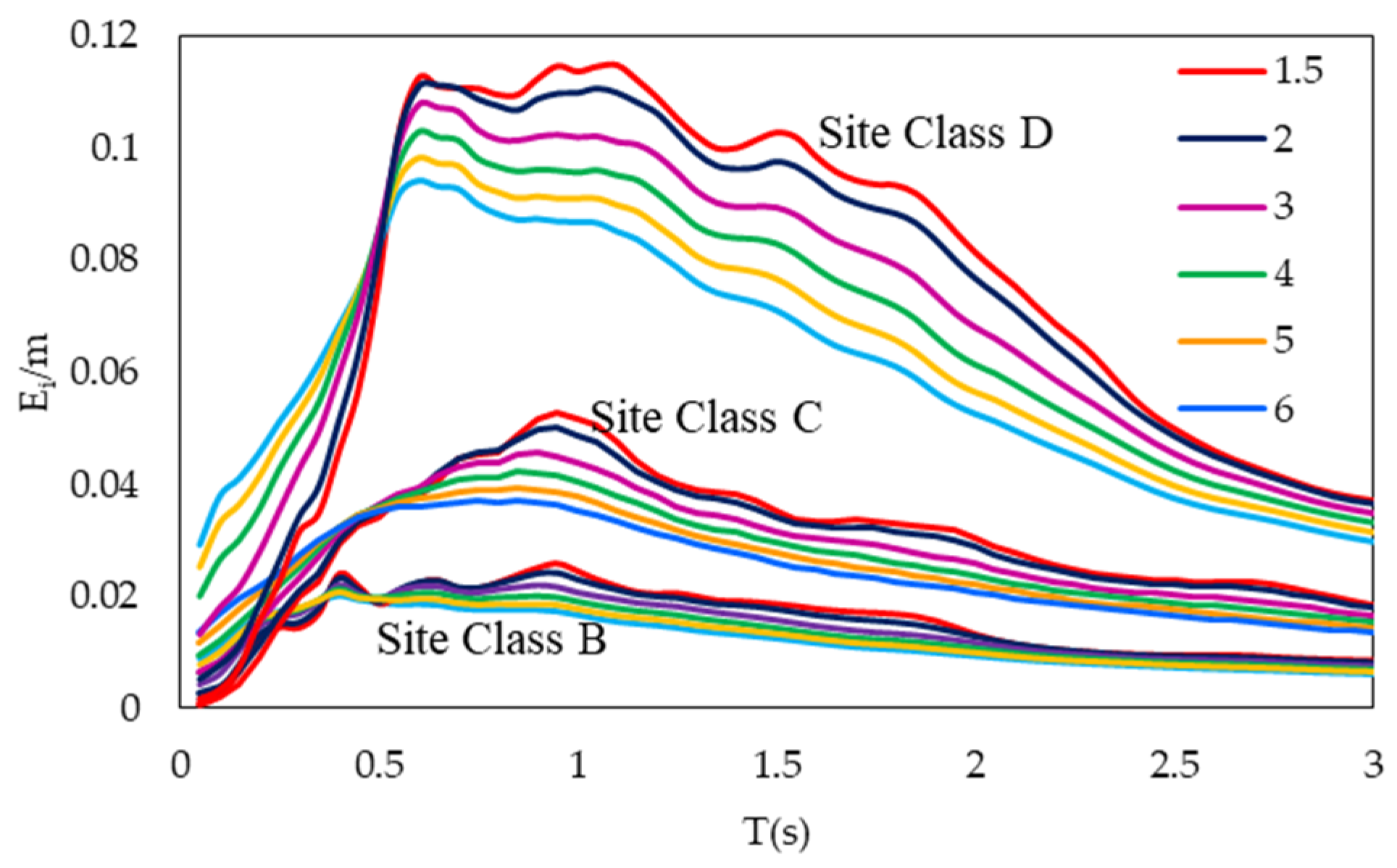
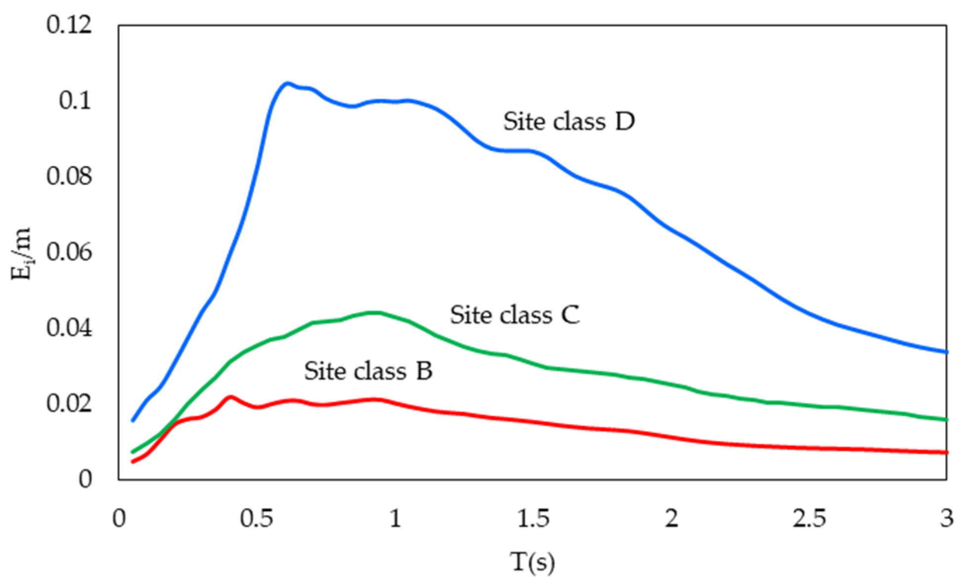
• The site class affects the input energy dissipated by an SDOF system. This effect influences the intensity rather than the shape of the input energy spectrum. Estimating the input energy velocity in terms of PSV helps to take this effect into consideration.
• Using normalized energy and period decreases the scatter at periods close to the characteristic period. (Figure 6)
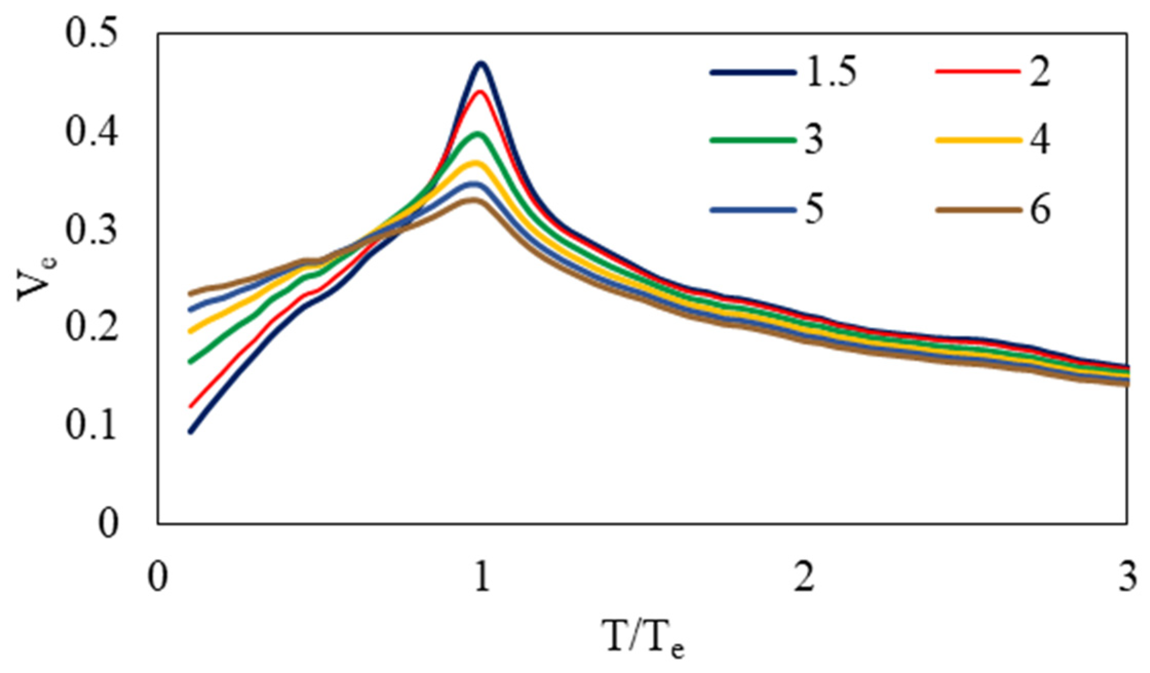
• The mean input energy velocity showed different trends in two spectral regions. It was observed that the input energy tends to decrease with increasing strength for systems with a period less than approximately 0.7 T_e and tend to increase for systems whose period higher than 0.7 T_e (Figure 8).
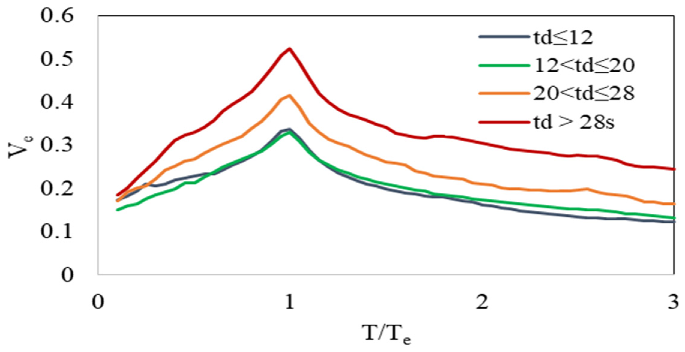
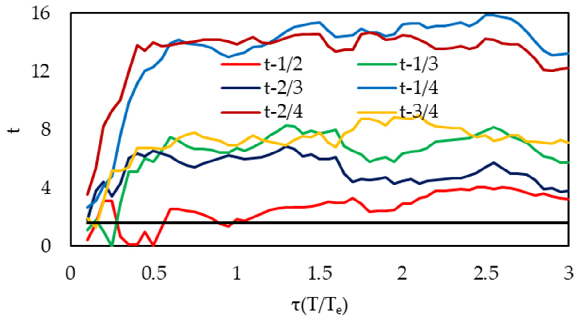
• Sensitivity analyses showed that the input energy velocity tends to increase on average as t_d increases. Furthermore, it was observed that the change in t_d is more effective on the input energy with increasing t_d (Figure 9).
• As seen from the correlation matrix, the spectrum intensity (SI) is more effective on input energy velocity than the other considered seismic parameters. The effect of spectrum intensity is taken into account in the estimation of input energy velocity by using an equation as a function of PSV, since spectrum intensity is the integration of PSV. Three different definitions of ground motion duration (t_d, t_d75, and t_uni) have been considered, and their correlation coefficients are very close to each other. This result shows a similar effect of all the considered ground motion duration parameters on input energy velocity.
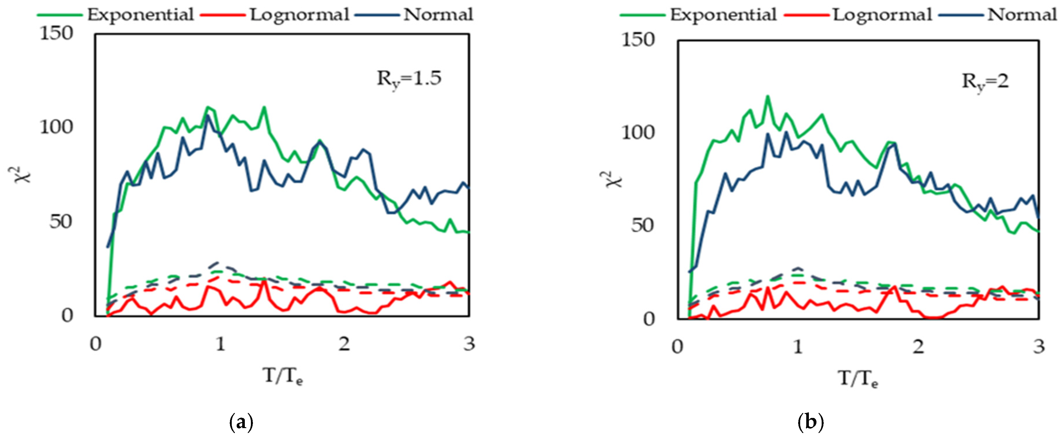
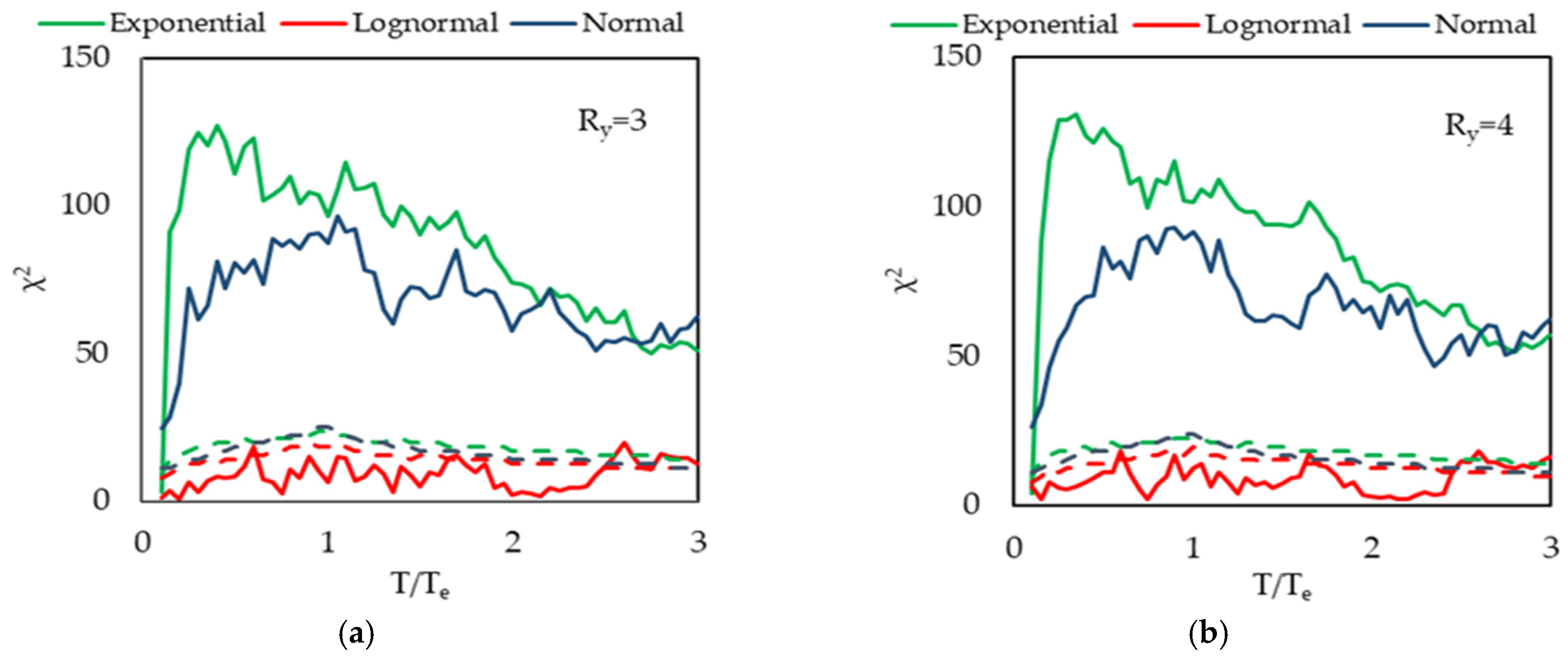
• The lognormal distribution was determined as the most reliable distribution model with the chi-square goodness-of-fit test for different strength reduction factor (R_y) and effective ground motion duration (t_d) groups, along the all T/T_e ranges (Figure 10, Figure 11, Figure 12, Figure 13 and Figure 14). The lognormal distribution has been previously verified by other researchers [21].
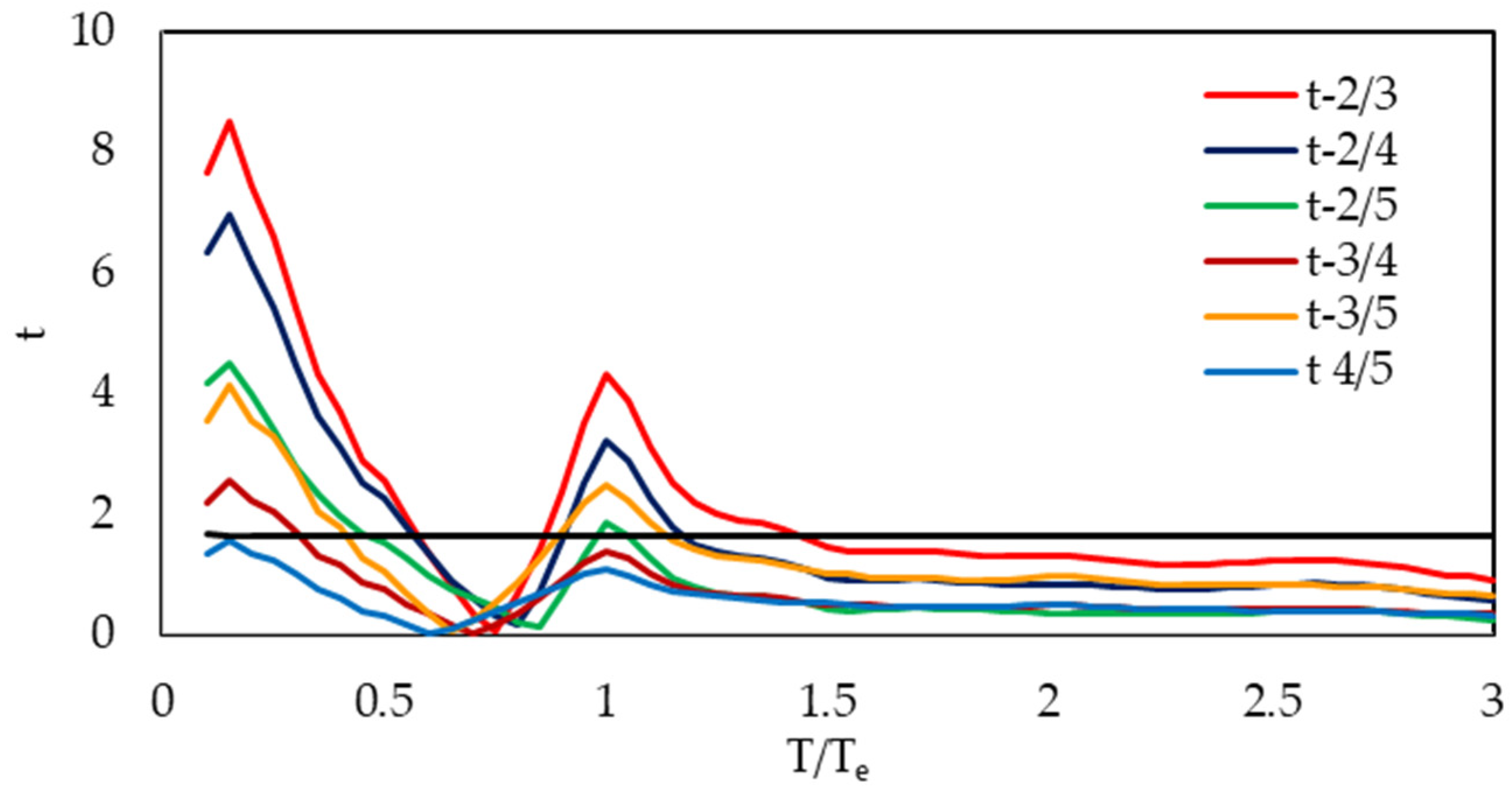
• The t-test and ANOVA results indicate that the mean V_e differs across different R_y groups over specific spectral ranges, except for group 4/5. According to hypothesis testing results at a 5% statistical significance level, strength influences input energy velocity within the ranges of 0.1T_e < T < 0.6T_e and 0.8T_e < T < 1.5T_e, except for group 4/5 (Figure 15 and Figure 16).
• Each considered R_y group, except group 4/5, has a threshold normalized period beyond which the effect of the strength reduction factor becomes negligible (0.35 s, 0.43 s, 0.45 s, and 0.6 s). The significant impact of strength on input energy velocity in the spectral region where the vibration period approximates the characteristic period suggests that it also plays a crucial role in determining the maximum input energy.
• Hypothesis test results show that the effective duration of ground motion (t_d) has an effect on the input energy velocity along almost all specific spectral ranges (Figure 17 and Figure 18).
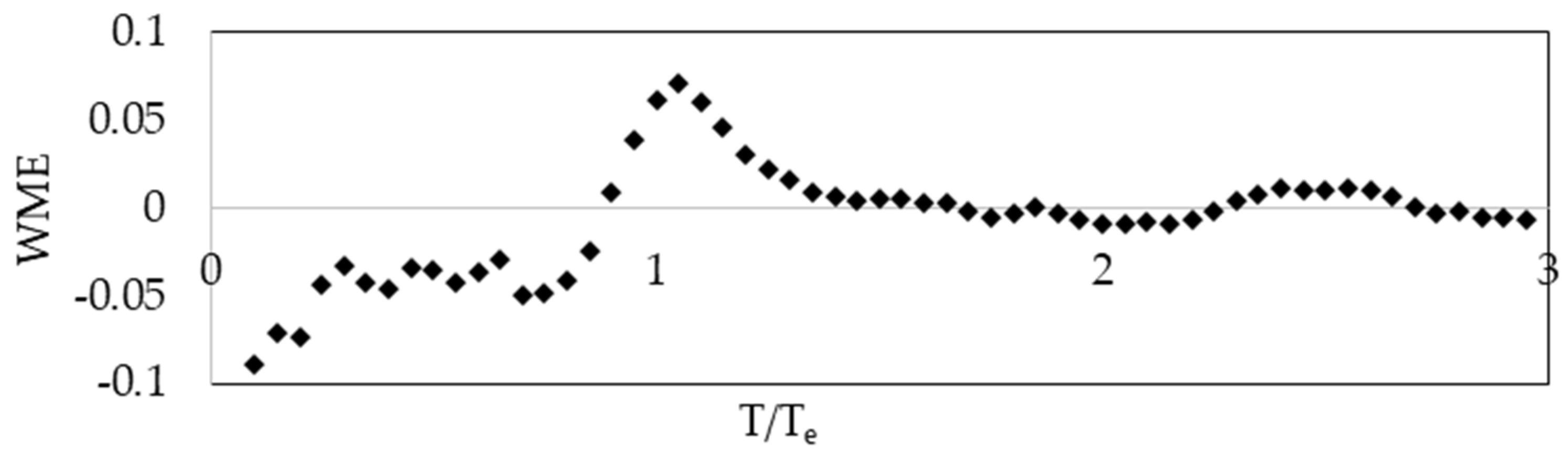
• The weighted mean error reaches the maximum value for very low periods (T < 0.3T_e) and periods approximately equal to T_e (Figure 20).
• The standard error of regression for estimating the input energy velocity is increasing with very low T/T_e ratios (Figure 21).
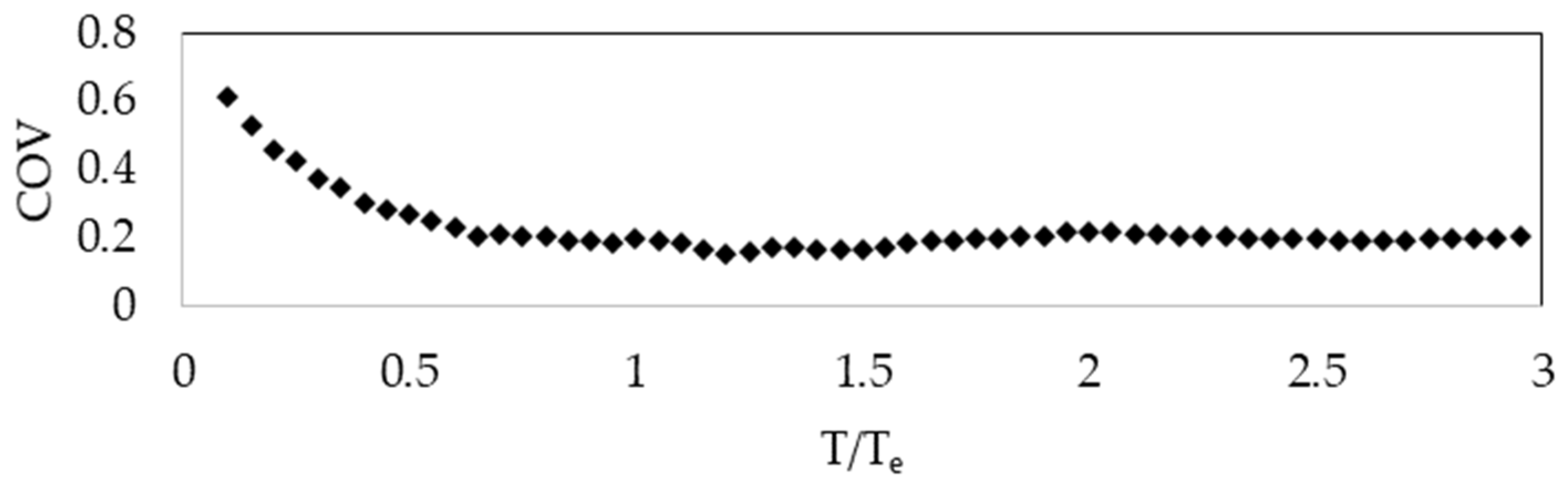
• The coefficient of variation for error of the proposed equation for estimating the input energy velocity is relatively higher in the short-period range (T < 0.5T_e), and the dispersion increases in this region as the T/T_e ratio decreases (Figure 22).

It is worth noting that all conclusions and observations drawn in this study are limited to SDOF systems with periods falling within the investigated period range.

References

1. Zahrah, T.; Hall, J. Earthquake energy absorption in SDOF structures. J. Struct. Eng. 1984, 110, 1757–1772. [Google Scholar] [CrossRef]
2. Akiyama, H. Earthquake-Resistant Limit-State Design for Buildings; The University of Tokyo Press: Tokyo, Japan, 1985. [Google Scholar]
3. Park, Y.J.; Ang, A.H.S. Mechanistic Seismic Damage Model for Reinforced Concrete. J. Struct. Eng. 1985, 111, 722–739. [Google Scholar] [CrossRef]
4. Cosenza, E.; Manfredi, G.; Ramasco, R. The use of damage functionals in earthquake engineering: A comparison between different methods. Earthq. Eng. Struc. Dyn. 1993, 22, 868–885. [Google Scholar] [CrossRef]
5. Fajfar, P.; Vidic, T. Consistent inelastic design spectra: Hysteretic and input energy. Earthq. Eng. Struct. Dyn. 1994, 23, 523–532. [Google Scholar] [CrossRef]
6. Chai, Y.H.; Fajfar, P.; Romstad, K.M. Formulation of duration-dependent inelastic seismic design spectrum. J. Struct. Eng. 1998, 124, 913–921. [Google Scholar] [CrossRef]
7. Manfredi, G. Evaluation of Seismic Energy Demand. Earthq. Eng. Struct. Dyn. 2001, 30, 485–499. [Google Scholar] [CrossRef]
8. Riddell, R.; Garcia, J.E. Hysteretic energy spectrum and damage control. Earthq. Eng. Struct. Dyn. 2001, 30, 1791–1816. [Google Scholar] [CrossRef]
9. Kunnath, S.K.; Chai, Y.H. Cumulative damage-based inelastic cyclic demand spectrum. Earthq. Eng. Struct. Dyn. 2004, 33, 499–520. [Google Scholar] [CrossRef]
10. Arroyo, D.; Ordaz, M. On the estimation of hysteretic energy demands for SDOF systems. Earthq. Eng. Struct. Dyn. 2007, 36, 2365–2382. [Google Scholar] [CrossRef]
11. Kazantzi, A.; Vavatsikos, D. The Hysteretic Energy as a Performance Measure in Analytical Studies. Earthq. Spect. 2018, 34, 719–739. [Google Scholar] [CrossRef]
12. Housner, G.W. Limit design of structures to resist earthquakes. In Proceedings of the 1st World Conference on Earthquake Engineering, Berkeley, CA, USA, 1956. [Google Scholar]
13. Mezgebo, M.G.; Lui, E.M. Hysteresis and Soil Site Dependent Input and Hysteretic Energy Spectra for Far-Source Ground Motions. Adv. Civ. Eng. 2016, 1548319, 1–29. [Google Scholar] [CrossRef]
14. Mezgebo, M.G.; Lui, E.M. A new methodology for energy-based seismic design of steel moment frames. Earthq. Eng. Eng. Vib. 2017, 16, 131–152. [Google Scholar] [CrossRef]
15. Homaei, F. Estimation of the ductility and hysteretic energy demands for soil–structure systems. Bull. Earthq. Eng. 2021, 19, 1365–1413. [Google Scholar] [CrossRef]
16. Hasanoğlu, S.; Güllü, E.; Güllü, A. Empirical correlations of constant ductility seismic input and hysteretic energies with conventional intensity measures. Bull. Earthq. Eng. 2023, 21, 4905–4922. [Google Scholar] [CrossRef]
17. Dindar, A.A.; Yalçin, C.; Yüksel, E.; Özkaynak, H.; Büyüköztürk, O. Development of Earthquake Energy Spectra. Earthq. Spect. 2015, 31, 1667–1689. [Google Scholar] [CrossRef]
18. Uang, C.M.; Bertero, V.V. Evaluation of seismic energy in structures. Earthq. Eng. Struct. Dyn. 1990, 19, 77–90. [Google Scholar] [CrossRef]
19. Nakashima, M.; Saburi, K.; Tsuji, B. Energy Input and Dissipation Behavior of Structures with Hysteretic Dampers. Earthq. Eng. Struct. Dyn. 1996, 19, 77–90. [Google Scholar]
20. Kuwamura, H.; Galambos, T.V. Earthquake Load for Structural Reliability. J. Struct. Eng. 1989, 115, 1446–1462. [Google Scholar] [CrossRef]
21. Güllü, A.; Yüksel, E.; Yalçin, C.; Dindar, A.A.; Özkaynak, H.; Büyüköztürk, O. An improved input energy spectrum verified by the shake table tests. Wiley 2019, 31, 1667–1689. [Google Scholar] [CrossRef]
22. Rahnama, M.; Krawinkler, H. Effects of Soft Soil and Hysteretic Model on Seismic Demands; Report No 108; John A. Blume Earthquake Engineering Center, Stanford University: Stanford, CA, USA, 1993. [Google Scholar]
23. Foutch, D.A.; Shi, S. Effects of hysteresis type on the seismic response of buildings. In Proceedings of the 6th U.S. National Conference on Earthquake Engineering, EERI, Seattle, WA, USA, 31 May–4 June 1998. [Google Scholar]
24. Huang, Z.; Foutch, D.A. Effect of hysteresis type on drift limit for global collapse of moment frame structures under seismic loads. J. Earthq. Eng. 2009, 13, 1363–2469. [Google Scholar] [CrossRef]
25. Ibarra, L.F.; Medina, R.A.; Krawinkler, H. Hysteretic models that incorporate strength and stiffness deterioration. Earthq. Eng. Struct. Dyn. 2005, 34, 1489–1511. [Google Scholar] [CrossRef]
26. Narges Gholami, N.; Garivani, S.; Askariani, S.S. State-of-the-Art Review of Energy-Based Seismic Design Methods. Arch. Comp. Methods Eng. 2021, 29, 1965–1996. [Google Scholar] [CrossRef]
27. Zhou, Y.; Song, G.; Huang, S.; Wu, H. Input energy spectra for self-centering SDOF systems. Soil Dyn. Earthq. Eng. 2019, 121, 293–305. [Google Scholar] [CrossRef]
28. Deniz, D.; Song, J.; Hajjar, J.F. Energy-based sidesway collapse fragilities for ductile structural frames under earthquake loadings. Eng. Struct. 2018, 174, 282–294. [Google Scholar] [CrossRef]
29. Bertero, V.V.; Mahin, S.A.; Herrera, R.A. Aseismic design implications of San Fernando earthquake records. Earthq. Eng. Struct. Dyn. 1978, 6, 31–42. [Google Scholar] [CrossRef]
30. Ambraseys, N.; Douglas, J. ESEE Report No. 00-4-Reapprasial of the Effect of Vertical Ground Motions on Response; Imperial College Civil and Environmental Department: London, UK, 2000. [Google Scholar]
31. FEMA 450 NEHRP Recommended Provisions for Seismic Regulations for New Buildings and Other Structures; Federal Emergency Management Agency: Washington, DC, USA, 2003.
32. Kuwamura, H.; Kirino, Y.; Akiyama, W. Prediction of earthquake energy input from smoothed Fourier amplitude spectrum. Earthq. Eng. Struct. Dyn. 1994, 23, 1125–1137. [Google Scholar] [CrossRef]
33. Ordaz, M.; Huerta, B.; Reinoso, E. Exact computation of input-energy spectra from Fourier amplitude spectra. Earthq. Eng. Struct. Dyn. 2003, 32, 597–605. [Google Scholar] [CrossRef]
34. Fajfar, P.; Vidic, T.; Fischinger, M. Seismic Design in Medium- and Long- Period Structures. Earthq. Eng. Struct. Dyn. 1989, 18, 1133–1144. [Google Scholar] [CrossRef]
35. Vidic, T.; Fajfar, P.; Fischinger, M. Consistent inelastic design spectra: Strength and displacement. Earthq. Eng. Struct. Dyn. 1994, 23, 507–521. [Google Scholar] [CrossRef]
36. Miranda, E.; Ruiz-Garcia, J. Influence of stiffness degradation on strength demands of structures built on soft soil sites. Eng. Struct. 2002, 24, 1271–1281. [Google Scholar] [CrossRef]
37. Ruiz-Garcia, J.; Miranda, E. Inelastic displacement ratios for design of structures on soft soil sites. ASCE J. Struct. Eng. 2004, 130, 2051–2061. [Google Scholar] [CrossRef]
38. Ruiz-Garcia, J.; Miranda, E. Inelastic displacement ratios for evaluation of existing structures. Earthq. Eng. Struct. Dyn. 2003, 32, 1237–1258. [Google Scholar] [CrossRef]
39. Miranda, E. Evaluation of site-dependent inelastic seismic design spectra. ASCE J. Struct. Eng. 1993, 119, 1319–1338. [Google Scholar] [CrossRef]
40. Hancıoğlu, B.; Polat, Z.; Kırçıl, M.S. Estimation of characteristic period for energy based seismic design. In Proceedings of the 2008 Seismic Engineering Conference Commemorating the 1908 Messina and Reggio Calabria Earthquake Parts 1–2, AIP Conference Proceedings, Reggio Calabria, Italy, 8–11 July 2008; Volume 1020, pp. 937–946. [Google Scholar]
41. Cosenza, E.; Manfredi, G. The improvement of the seismic-resistant design for existing and new structures using damage criteria. In Proceedings of the International Workshop on Seismic Design Methodologies for the Next Generation of Codes, Balkema, Bled, Slovenia, 24–27 June 1997; pp. 1–31. [Google Scholar]
42. Somerville, P.G.; Smith, N.F.; Graves, R.W.; Abrahamson, N.A. Modification of empirical strong ground motion attenuation relations to include the amplitude and duration effects of rupture directivity. Seismol. Res. Lett. 1997, 68, 199–222. [Google Scholar] [CrossRef]
43. Trifunac, M.D.; Brady, A.G. A Study on the Duration of Strong Earthquake Ground Motion. Bull. Seismol. Soc. Am. 1975, 65, 581–626. [Google Scholar]
44. Bolt, B.A. Duration of strong ground motions. In Proceedings of the Fifth World Conference on Earthquake Engineering, Rome, Italy, 25–29 June 1973; Volume 1, pp. 1304–1313. [Google Scholar]
45. Ang, A.H.S.; Tang, W.H. Probability Concepts in Engineering Planning and Design, Basic Principles-Vol. 1; Wiley: Toronto, ON, Canada, 1975. [Google Scholar]
46. Sucuoğlu, H.; Yücemen, S.; Gezer, A.; Erberik, A. Statistical evaluation of the damage potential of earthquake ground motions. Struct. Saf. 1998, 20, 357–378. [Google Scholar] [CrossRef]
47. StatSoft Inc. Electronic Statistics Textbook. Tulsa OK. Available online: http://www.statsoft.com/-textbook/stathome.html (accessed on 1 April 2008).
Figure 1. Force-displacement relationship of an elastoplastic SDOF system and its mechanical model.
Buildings 15 02288 g001
Figure 2. Input energy spectrum (drawn schematically).
Buildings 15 02288 g002
Figure 3. Input energy spectra of an SDOF systems for different strength levels and site classes.
Buildings 15 02288 g003
Figure 4. Mean input energy spectra for different strength reduction factors (Ry) for each site class.
Buildings 15 02288 g004
Figure 5. Mean input energy spectra of each considered site class.
Buildings 15 02288 g005
Figure 6. Normalized input energy spectra of SDOF systems for different strength reduction factors (Ry) and site classes.
Buildings 15 02288 g006
Figure 7. Normalized input energy spectra of SDOF systems for different strength levels and site classes.
Buildings 15 02288 g007
Figure 8. Mean spectra of Ve (m/s) for the systems categorized by Ry.
Buildings 15 02288 g008
Figure 9. Mean spectra of Ve (m/s) for the ground motions categorized td.
Buildings 15 02288 g009
Figure 10. The spectra of chi-square goodness-of-fit test results of Ve for different ground motions classified according to Ry: (a) 1.5; (b) 2.
Buildings 15 02288 g010
Figure 11. The spectra of chi-square goodness-of-fit test results of Ve for different ground motions classified according to Ry: (a) 3; (b) 4.
Buildings 15 02288 g011
Figure 12. The spectra of chi-square goodness-of-fit test results of Ve for different ground motions classified according to Ry: (a) 5; (b) 6.
Buildings 15 02288 g012
Figure 13. The spectra of chi-square goodness-of-fit test results of Ve for different ground motions classified according to td: (a) td ≤ 12 s; (b) 12 s < td ≤ 20 s.
Buildings 15 02288 g013
Figure 14. The spectra of chi-square goodness-of-fit test results of Ve for different ground motions classified according to td: (a) 20 s < td ≤ 28 s; (b) 28 s < td.
Buildings 15 02288 g014
Figure 15. The spectra of t-test results of the logarithmic values of Ve for Ry groups.
Buildings 15 02288 g015
Figure 16. The spectra of ANOVA of the logarithmic of Ve values for Ry groups.
Buildings 15 02288 g016
Figure 17. The spectra of t-test results of the logarithmic values of Ve for td groups.
Buildings 15 02288 g017
Figure 18. The spectra of ANOVA results of the logarithmic values of Ve for td groups.
Buildings 15 02288 g018
Figure 19. The scatter plot of Ve for 0.1 ≤ T/Te ≤ 3.0.
Buildings 15 02288 g019
Figure 20. Weighted mean error of regression.
Buildings 15 02288 g020
Figure 21. Root mean squared error of regression.
Buildings 15 02288 g021
Figure 22. Coefficient of variation of error of regression.
Buildings 15 02288 g022