
Study on Piping Layout Optimization for Chiller-Plant Rooms Using an Improved A* Algorithm and Building Information Modeling: A Case Study of a Shopping Mall in Qingdao

Abstract
1. Introduction
1.1. Literature Review
1.1.1. HVAC Piping Network Optimization
1.1.2. Automatic Pipeline Routing Algorithm
1.1.3. Retrofitting of Existing HVAC Systems
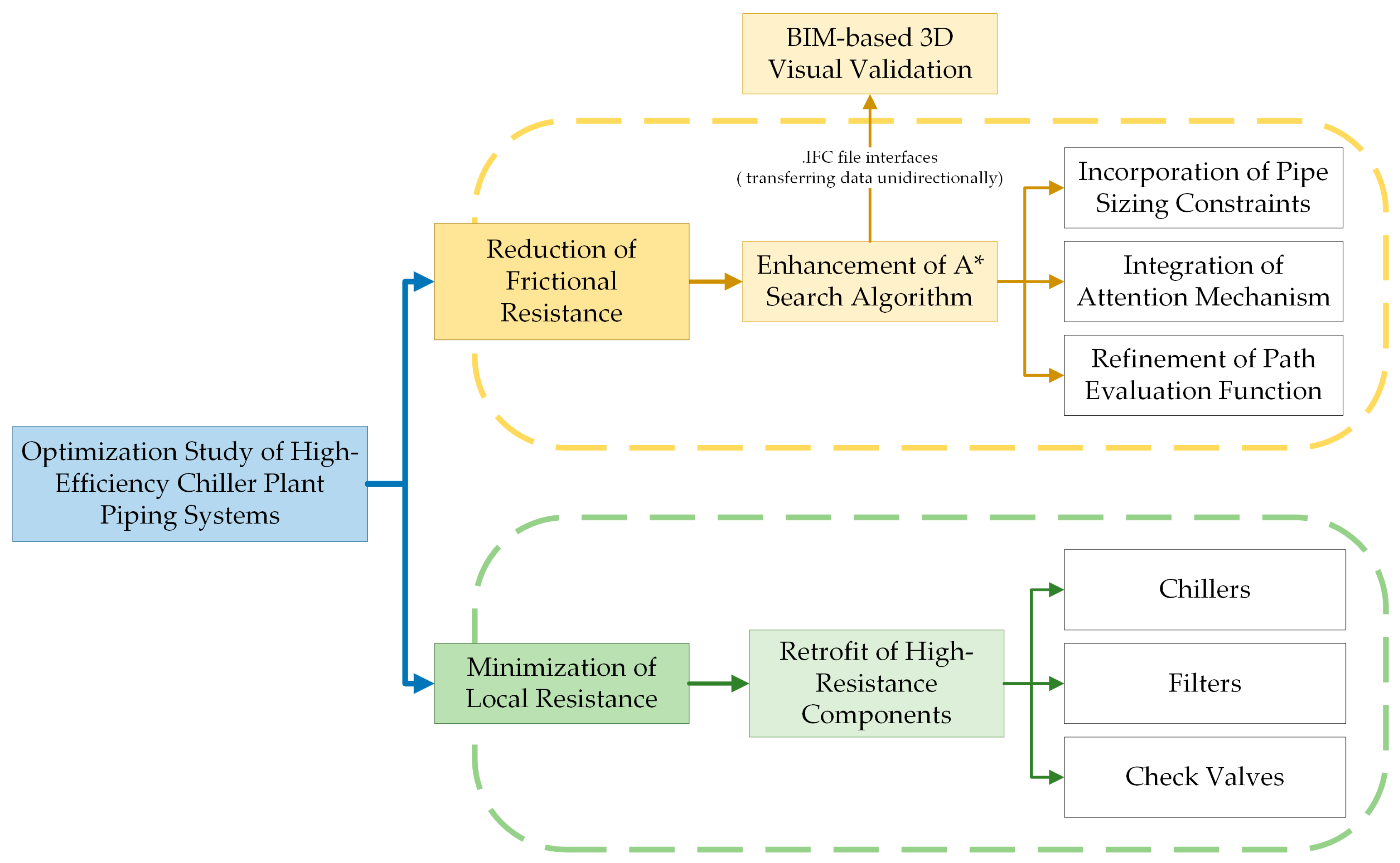
1.2. The Main Aspects and Innovations
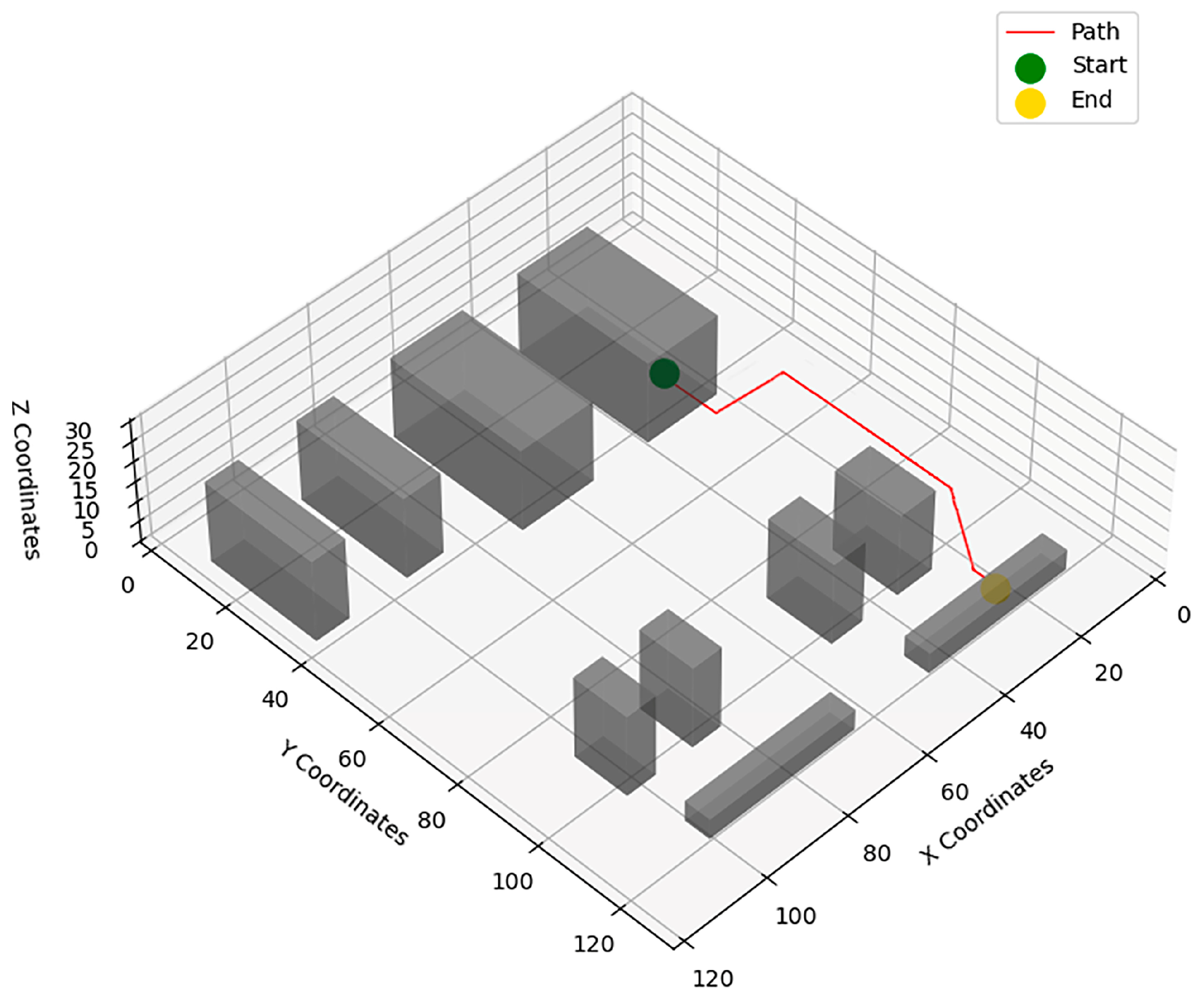
- Path-planning algorithm enhancement: PBZ safety penalties, an attention-weighted heuristic, and a turn-penalty cost enable 98.6% safety-margin compliance on a 120 × 120 × 30 grid while remaining 68% faster than Dijkstra and two orders faster than PSO.
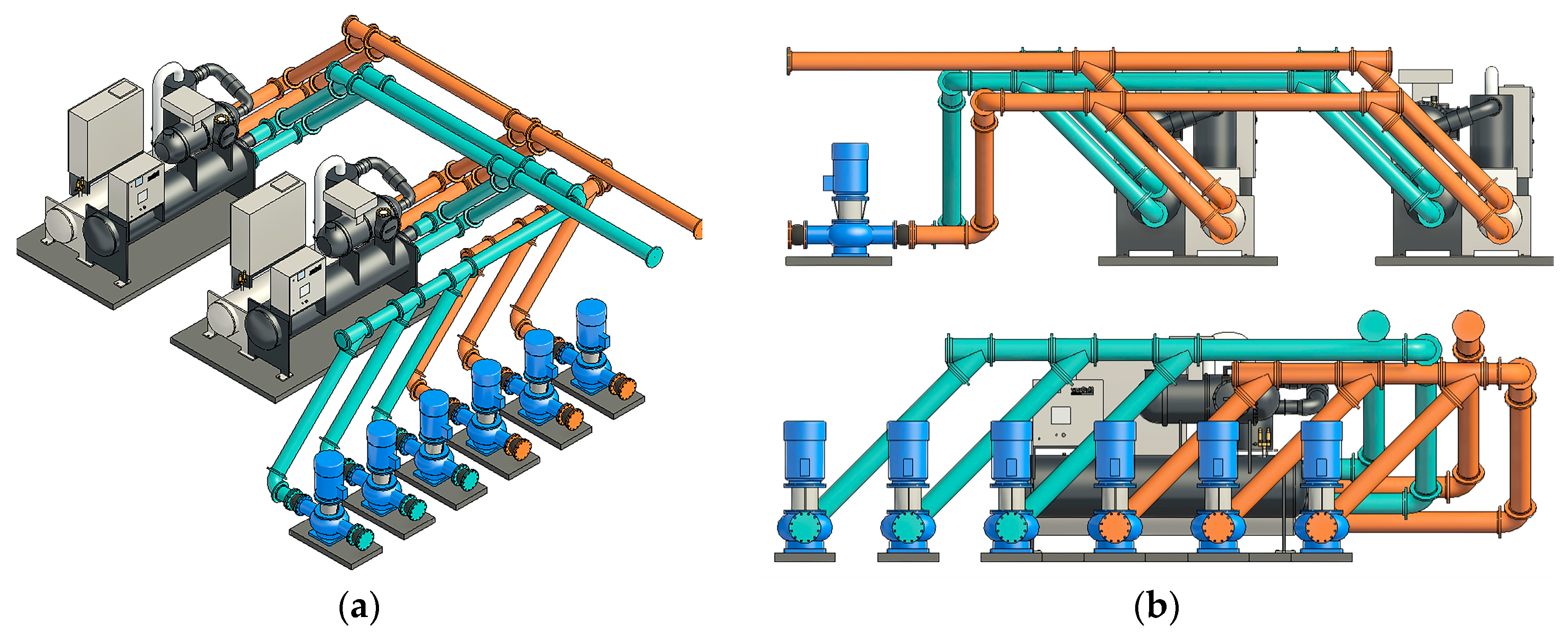
- 3-D modeling and visual clash verification: An automated IFC interface converts algorithmic paths into BIM objects, allowing instant collision checking and intuitive visualization inside Revit.
- Reselection of high-resistance components: Magnetic-bearing chillers, cylindrical strainers, and tilted-disc check valves replace legacy units, reducing local pressure losses by up to 50.8% and synergizing with the smoother pipeline.
- Engineering validation and economic appraisal: In the shopping-mall case, system resistance falls by 239.7 kPa (−47.7%), pump-energy use and maintenance costs drop by 47.7% and 75%, respectively, and a life-cycle cost analysis confirms strong financial viability.
2. Materials and Methods
2.1. Improved A* Algorithm
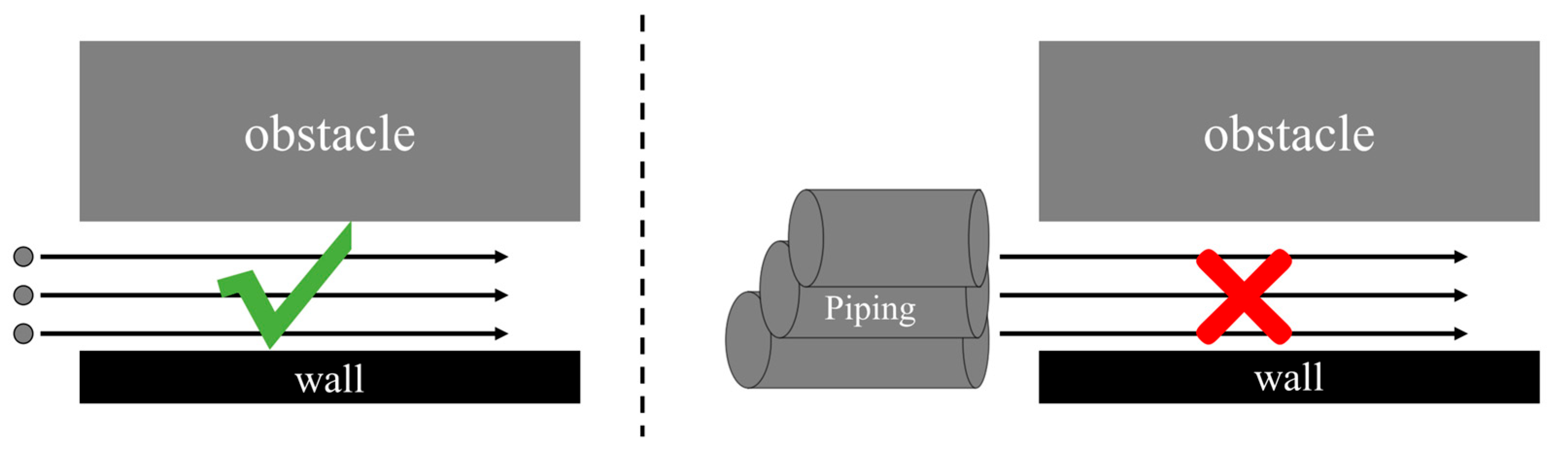
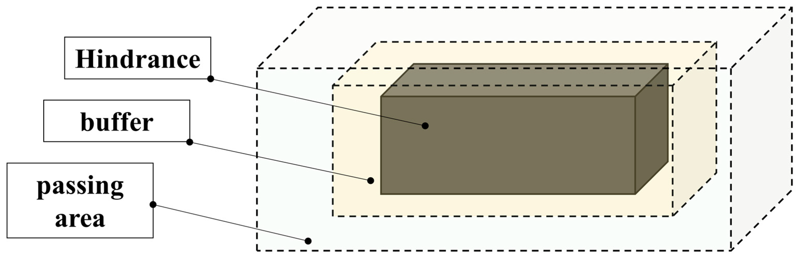
2.1.1. Path Planning with Buffer Protection
2.1.2. Introduction of Attention Mechanisms
2.1.3. Turn Optimization
2.1.4. Development of an Automated Interface Between Path Planning and BIM
2.1.5. Computational Complexity Analysis
2.1.6. Parametric Sensitivity Analysis
2.1.7. Algorithm Benchmarking
2.2. Optimizing Local Resistance in Chiller-Plant Rooms
2.2.1. Optimization of Chiller-Plant Selection
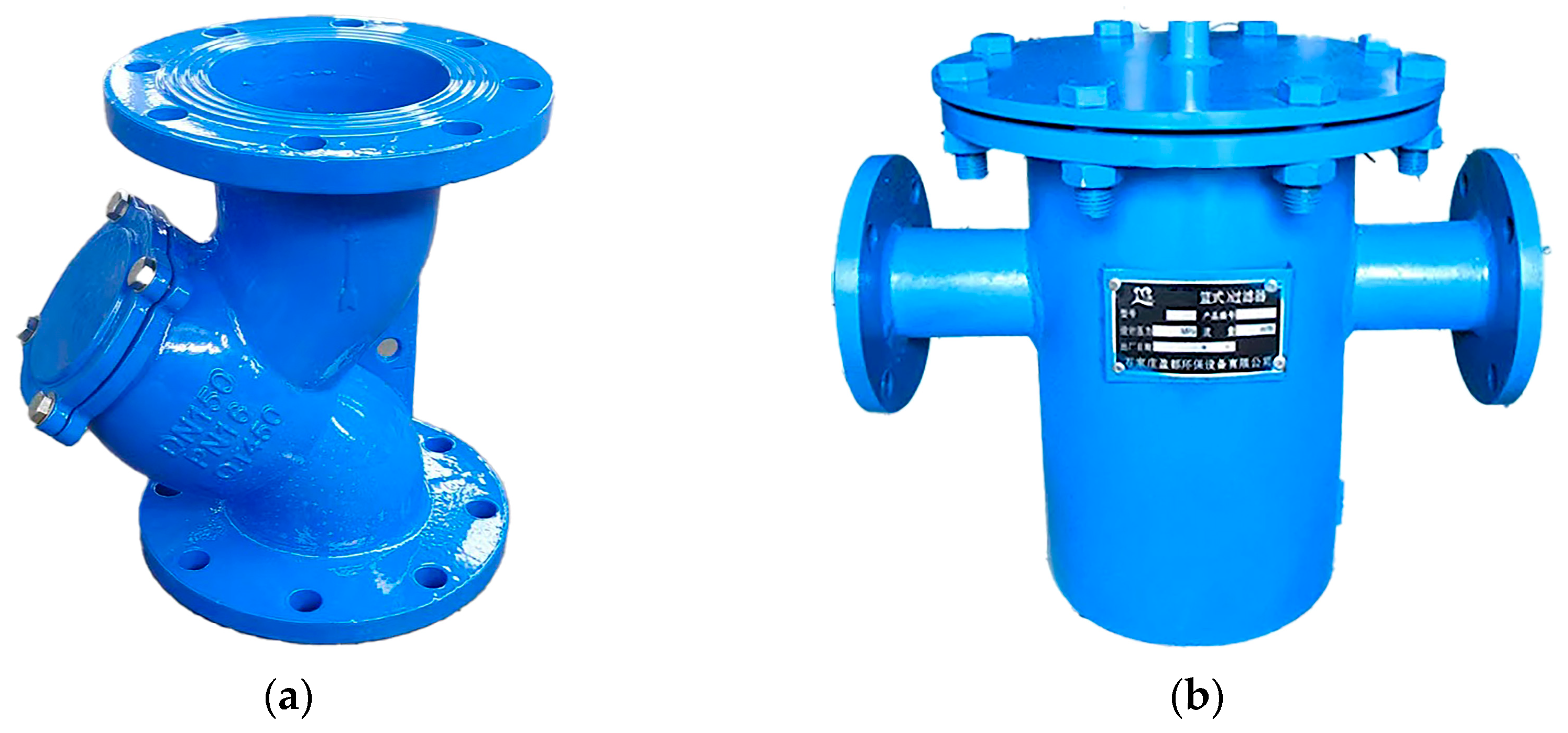
2.2.2. Optimization of Filter Selection
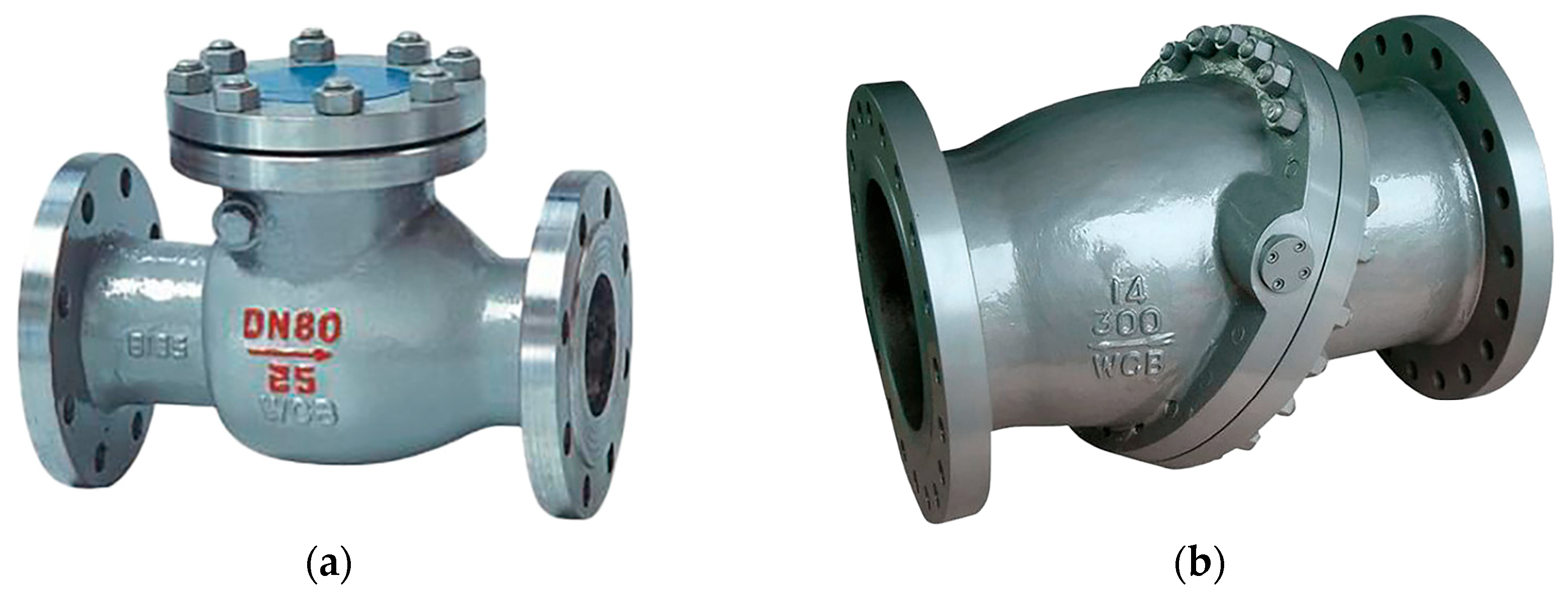
2.2.3. Optimization of Check Valve Selection
2.2.4. Life-Cycle Cost Analysis Framework
3. Case Study
3.1. Project Background
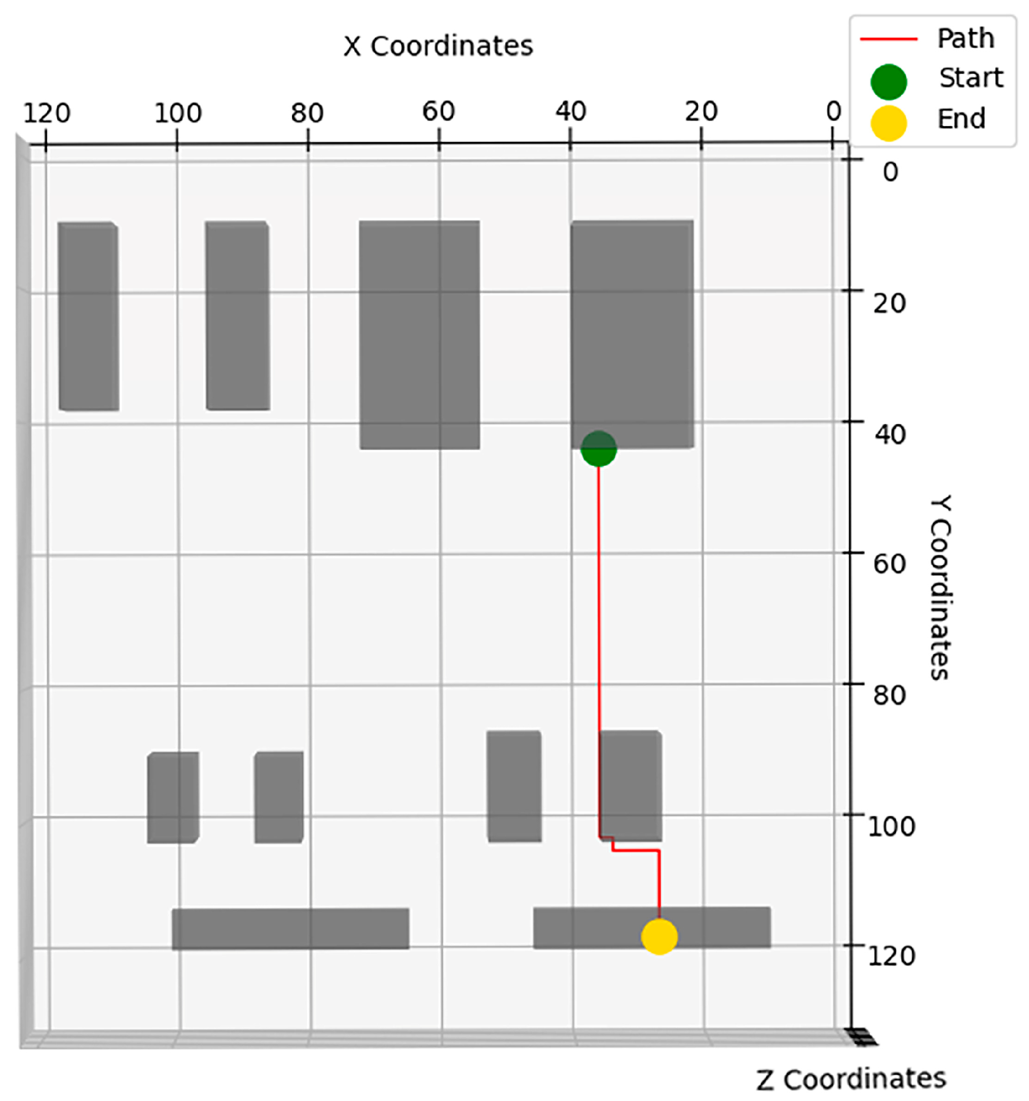
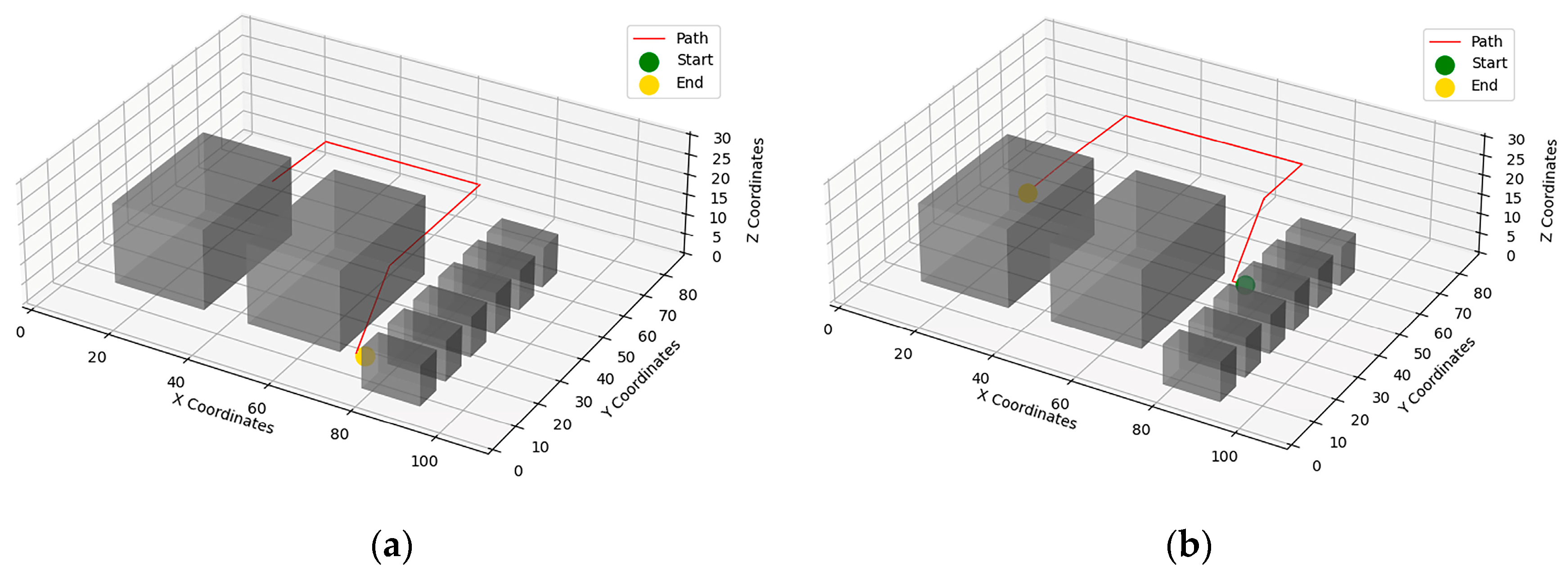
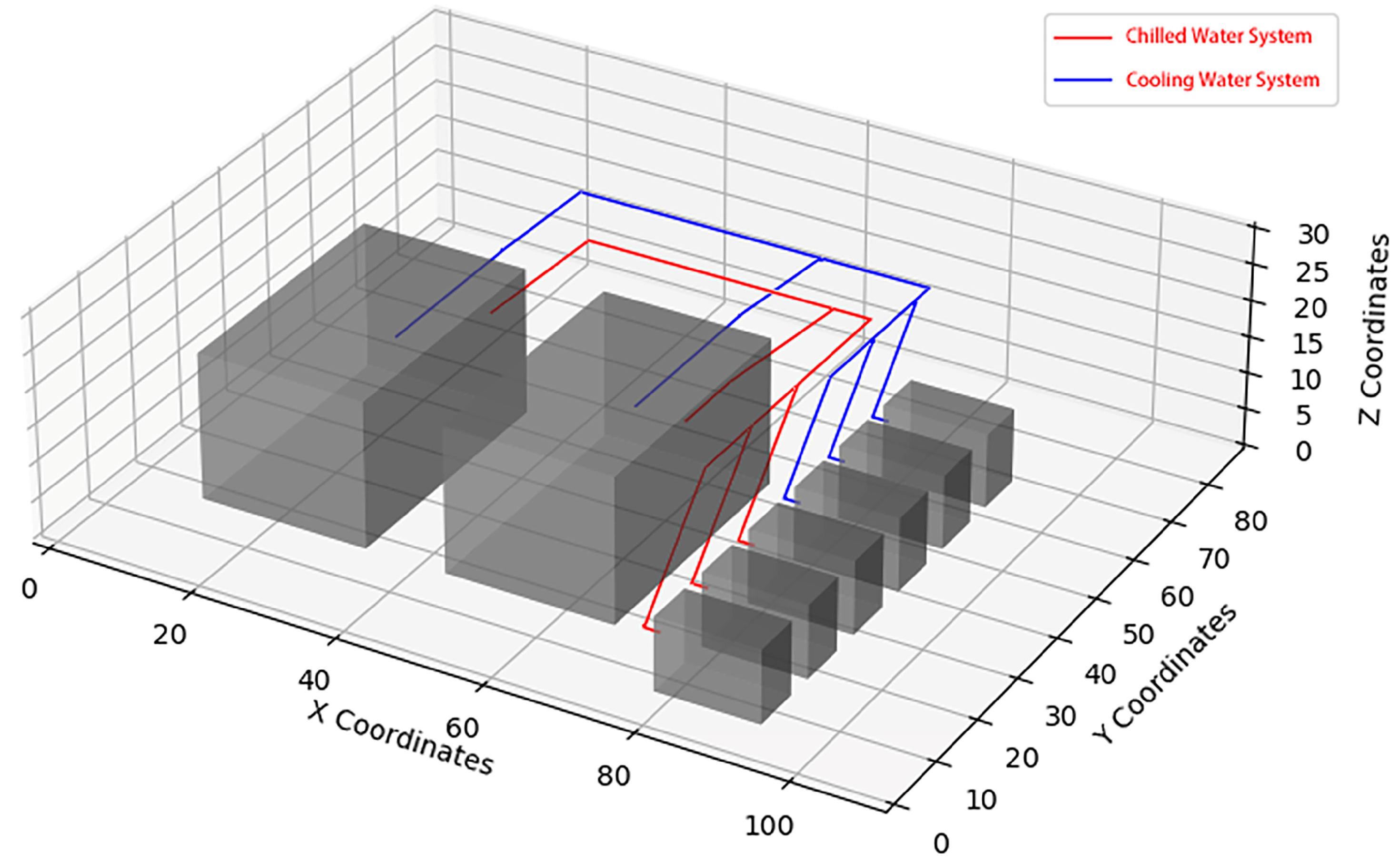
3.2. Pipeline Path Planning
3.3. Optimization of Refrigeration System Components
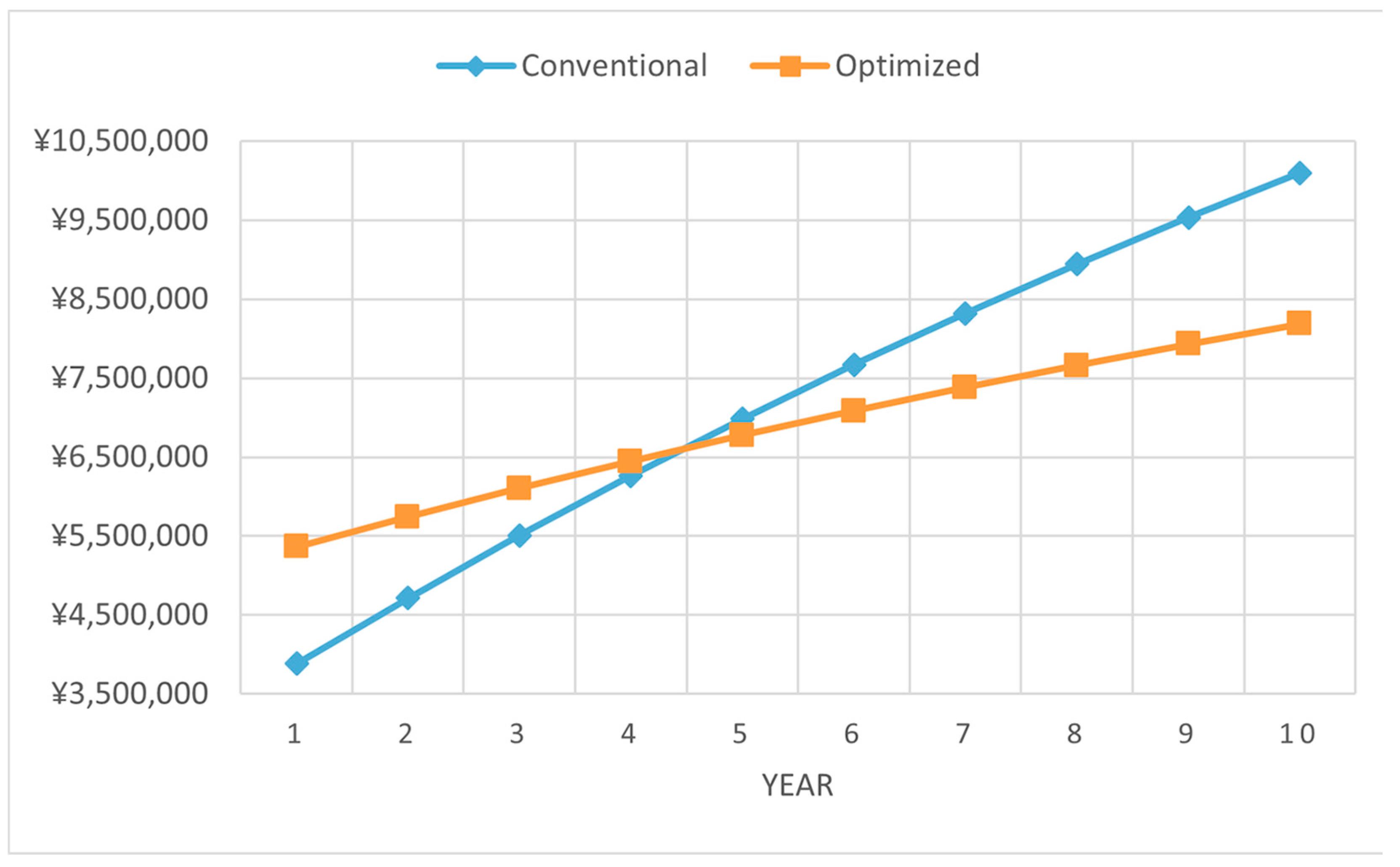
3.4. Life-Cycle Cost Analysis of Equipment Replacement
3.5. Comparison of Piping Resistance in the Server Room Before and After Optimization
4. Discussion and Conclusions
- Introduces Protective Buffer Zones (PBZ) to prevent collisions, a strategy applicable to any confined equipment room layout;
- Employs an attention mechanism to reserve maintenance space, addressing a universal need for operational accessibility;
- Prioritizes 135° large-angle elbows to minimize flow resistance, a hydraulic optimization principle transferable to all piping systems.
4.1. Method Generalizability and Limitations
- Algorithmic adaptability: PBZ safety margins (), attention weights (, ), and turn penalties are user-configurable parameters, enabling adaptation to spatial constraints in hospitals (strict clearance needs), data centers (high-density layouts), or retrofits (legacy space limitations);
- Component optimization universality: Resistance reduction via equipment reselection (Section 2.2) relies on standard hydraulic properties, not building-specific factors.
- Computational efficiency of the improved A* algorithm was validated for a 110 × 88 × 30 grid space with ten obstacles, but its performance in hyper-complex systems (e.g., multi-chiller plants with 50+ obstacles or irregular geometries) remains untested;
- Current research focuses primarily on path optimization for standard refrigeration systems, where computational efficiency for complex system path generation requires further enhancement;
4.2. Future Work
- Cross-building validation demonstrates its adaptability by implementing the method across diverse critical infrastructures: hospitals, data centers, retrofit projects, etc.;
- Significantly improving computational efficiency, particularly processing speed, for hyper-complex systems;
- To enhance credibility, we are committed to conducting field measurements by installing pressure sensors at pump inlets/outlets and critical nodes within the retrofitted mall system. This will enable a direct comparison of pump power consumption before and after optimization (scheduled completion: December 2025);
- Develop self-adaptive learning algorithms for parameters to enhance generalizability.
Author Contributions
Funding
Data Availability Statement
Conflicts of Interest
References
- Enteria, N.; Mizutani, K. The Role of the Thermally Activated Desiccant Cooling Technologies in the Issue of Energy and Environment. Renew. Sustain. Energy Rev. 2011, 15, 2095–2122. [Google Scholar] [CrossRef]
- Alonso, S.; Morán, A.; Prada, M.Á.; Reguera, P.; Fuertes, J.J.; Domínguez, M. A Data-Driven Approach for Enhancing the Efficiency in Chiller Plants: A Hospital Case Study. Energies 2019, 12, 827. [Google Scholar] [CrossRef]
- Katsoyiannis, A.; Cincinelli, A. ‘Cocktails and Dreams’: The Indoor Air Quality That People Are Exposed to While Sleeping. Curr. Opin. Environ. Sci. Health 2019, 8, 6–9. [Google Scholar] [CrossRef]
- Huang, X.; Yan, J.; Zhou, X.; Shen, A.; Yang, Z. Optimization Strategy for Minimizing Energy Consumption of Air Conditioning Terminal System in the Internet Data Center. J. Build. Eng. 2024, 96, 110315. [Google Scholar] [CrossRef]
- Kim, H.-J.; Cho, Y.-H. Optimization of Supply Air Flow and Temperature for VAV Terminal Unit by Artificial Neural Network. Case Stud. Therm. Eng. 2022, 40, 102511. [Google Scholar] [CrossRef]
- Yu, J.; Liu, Q.; Zhao, A.; Chen, S.; Gao, Z.; Wang, F.; Zhang, R. A Distributed Optimization Algorithm for the Dynamic Hydraulic Balance of Chilled Water Pipe Network in Air-Conditioning System. Energy 2021, 223, 120059. [Google Scholar] [CrossRef]
- Wang, H.; Wang, H.; Zhu, T. A New Hydraulic Regulation Method on District Heating System with Distributed Variable-Speed Pumps. Energy Convers. Manag. 2017, 147, 174–189. [Google Scholar] [CrossRef]
- Wijaya, T.K.; Sholahudin; Alhamid, M.I.; Saito, K.; Nasruddin, N. Dynamic Optimization of Chilled Water Pump Operation to Reduce HVAC Energy Consumption. Therm. Sci. Eng. Prog. 2022, 36, 101512. [Google Scholar] [CrossRef]
- Blokland, M.; van der Mei, R.D.; Pruyn, J.F.J.; Berkhout, J. Literature Survey on Automatic Pipe Routing. Oper. Res. Forum 2023, 4, 35. [Google Scholar] [CrossRef]
- Ulum, U.I.P.M.; Santi, I.H.; Chulkamdi, M.T. Implementation of Dijkstra Algorithm in Determining the Fastest Route for Goods Delivery. J. Artif. Intell. Eng. Appl. JAIEA 2025, 4, 1443–1449. [Google Scholar] [CrossRef]
- Gunawan; Hamada, K.; Kunihiro, K.; Utomo, A.S.A.; Ahli, M.; Lesmana, R.; Cornelius; Kobayashi, Y.; Yoshimoto, T.; Shimizu, T. Automated Pipe Routing Optimization for Ship Machinery. J. Mar. Sci. Appl. 2022, 21, 170–178. [Google Scholar] [CrossRef]
- Liang, R.; Wang, C.; Wang, P.; Yoon, S. Realization of Rule-Based Automated Design for HVAC Duct Layout. J. Build. Eng. 2023, 80, 107946. [Google Scholar] [CrossRef]
- Lu, Y.; Da, C. Global and Local Path Planning of Robots Combining ACO and Dynamic Window Algorithm. Sci. Rep. 2025, 15, 9452. [Google Scholar] [CrossRef] [PubMed]
- Zhai, L.; Feng, S. A Novel Evacuation Path Planning Method Based on Improved Genetic Algorithm. J. Intell. Fuzzy Syst. 2021, 42, 1813–1823. [Google Scholar] [CrossRef]
- Yu, Z.; Si, Z.; Li, X.; Wang, D.; Song, H. A Novel Hybrid Particle Swarm Optimization Algorithm for Path Planning of UAVs. IEEE Internet Things J. 2022, 9, 22547–22558. [Google Scholar] [CrossRef]
- Ayawli, B.B.K.; Chellali, R.; Appiah, A.Y.; Kyeremeh, F. An Overview of Nature-Inspired, Conventional, and Hybrid Methods of Autonomous Vehicle Path Planning. J. Adv. Transp. 2018, 2018, 8269698. [Google Scholar] [CrossRef]
- Liu, H.; Zhang, Y. ASL-DWA: An Improved A-Star Algorithm for Indoor Cleaning Robots. IEEE Access 2022, 10, 99498–99515. [Google Scholar] [CrossRef]
- Wang, D.; Liu, B.; Jiang, H.; Liu, P. Path Planning for Construction Robot Based on the Improved A* Algorithm and Building Information Modeling. Buildings 2025, 15, 719. [Google Scholar] [CrossRef]
- Duchoň, F.; Babinec, A.; Kajan, M.; Beňo, P.; Florek, M.; Fico, T.; Jurišica, L. Path Planning with Modified a Star Algorithm for a Mobile Robot. Procedia Eng. 2014, 96, 59–69. [Google Scholar] [CrossRef]
- Liu, C.; Sharples, S.; Mohammadpourkarbasi, H. A Review of Building Energy Retrofit Measures, Passive Design Strategies and Building Regulation for the Low Carbon Development of Existing Dwellings in the Hot Summer–Cold Winter Region of China. Energies 2023, 16, 4115. [Google Scholar] [CrossRef]
- Paven, A.C.; Ion, M.; Carutasu, G. Decision Support Systems for Buildings Energy Efficiency. ACTA Tech. Napoc.—Ser. Appl. Math. Mech. Eng. 2021, 64(1-S1), 253–260. [Google Scholar]
- AMINI Toosi, H.; Lavagna, M.; Leonforte, F.; Del Pero, C.; Aste, N. Life Cycle Sustainability Assessment in Building Energy Retrofitting; A Review. Sustain. Cities Soc. 2020, 60, 102248. [Google Scholar] [CrossRef]
- Ardente, F.; Beccali, M.; Cellura, M.; Mistretta, M. Energy and Environmental Benefits in Public Buildings as a Result of Retrofit Actions. Renew. Sustain. Energy Rev. 2011, 15, 460–470. [Google Scholar] [CrossRef]
- Iwuanyanwu, O.; Gil-Ozoudeh, I.; Okwandu, A.C.; Ike, C.S. Retrofitting Existing Buildings for Sustainability: Challenges and Innovations. Eng. Sci. Technol. J. 2024, 5, 2616–2631. [Google Scholar] [CrossRef]
- Dai, Y.; Liu, J.; Zou, S. Energy-Saving and Economic Analysis of the Data Center Cooling System Using Magnetic Bearing Chillers under Different Climate Conditions. Case Stud. Therm. Eng. 2024, 61, 104915. [Google Scholar] [CrossRef]
- Milenković, I.M.; Reljić, V.L.; Dudić, S.P.; Mladenović, V.S. Energy Efficient Compressed Air Filtration: An Experimental Study on the Effect of Filters Selection and Configuration on Pressure Drop. Therm. Sci. 2024, 28, 377–389. [Google Scholar] [CrossRef]
- Gobinath, P.; Crawford, R.H.; Traverso, M.; Rismanchi, B. Life Cycle Energy and Greenhouse Gas Emissions of a Traditional and a Smart HVAC Control System for Australian Office Buildings. J. Build. Eng. 2024, 82, 108295. [Google Scholar] [CrossRef]
- Scislo, L.; Szczepanik-Scislo, N. Near Real-Time Access Monitoring Based on IoT Dynamic Measurements of Indoor Air Pollutant. In Proceedings of the 2023 IEEE 12th International Conference on Intelligent Data Acquisition and Advanced Computing Systems: Technology and Applications (IDAACS), Dortmund, Germany, 7–9 September 2023; Volume 1, pp. 729–734. [Google Scholar]
- da Costa, G.C.L.R.; Figueiredo, S.H.; Ribeiro, S.E.C. Estudo Comparativo da Tecnologia CAD com a Tecnologia BIM. Rev. Ensino Eng. 2015, 34, 11–18. [Google Scholar] [CrossRef]
- Cao, Y.; Kamaruzzaman, S.N.; Aziz, N.M. Green Building Construction: A Systematic Review of BIM Utilization. Buildings 2022, 12, 1205. [Google Scholar] [CrossRef]
- Ye, Z.; Antwi-Afari, M.F.; Tezel, A.; Manu, P. Building Information Modeling (BIM) in Project Management: A Bibliometric and Science Mapping Review. Eng. Constr. Archit. Manag. 2024, 32, 3078–3103. [Google Scholar] [CrossRef]


| Obstacle Number | Obstacle Coordinates | Equipment Name |
|---|---|---|
| 1 | Chiller 1 | |
| 2 | Chiller 2 | |
| 3 | Plate Type Heat Exchanger 1 | |
| 4 | Plate Type Heat Exchanger 2 | |
| 5 | Chilled Water Pumps 1 | |
| 6 | Chilled Water Pumps 2 | |
| 7 | Cooling Water Pumps 1 | |
| 8 | Cooling Water Pumps 2 | |
| 9 | Water Separator 1 | |
| 10 | Water Separator 2 |
| The Value of γ | Meaning |
|---|---|
| Large | Extremely prioritizes avoiding the Buffer Zone, even if it requires a significantly longer detour to guarantee safety clearance. Paths will be longer but offer absolute safety. |
| Medium | Attempts to follow shorter paths. However, if a short path comes too close to obstacles (entering the Buffer Zone), the increased penalty makes it “appear” longer in the cost evaluation. Consequently, it is replaced by a safer alternative path. |
| Small | Paths resemble those generated by the original A* algorithm. This may result in paths passing close to obstacles (if that path is indeed the shortest). Safety guarantees are weaker. |
| Infinity | Equivalent to treating the Buffer Zone as an impassable area (hard constraint). The path cost for any path entering the Buffer Zone becomes infinite, effectively prohibiting it entirely. |
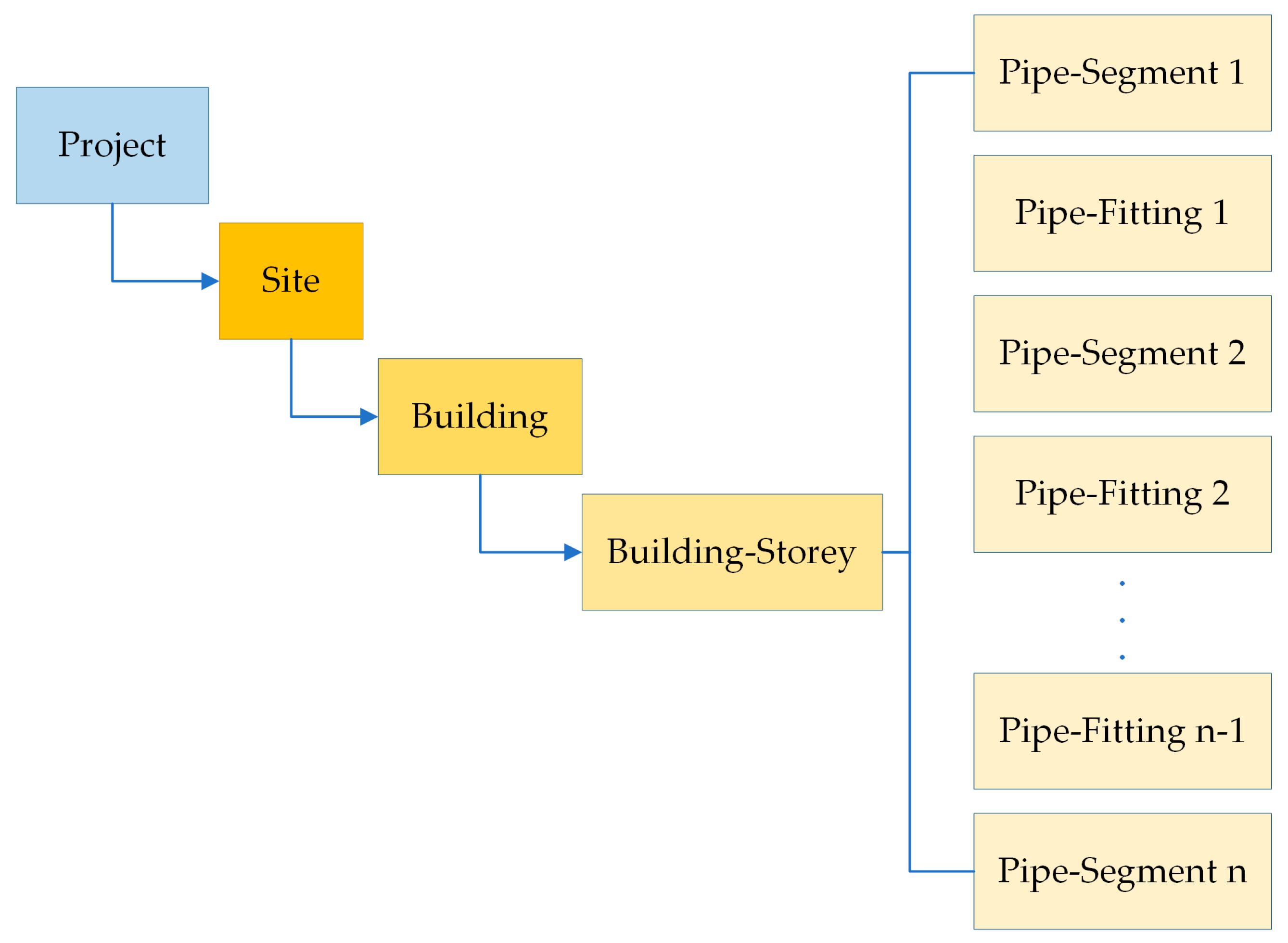
| Level | IFC Entity Type | Purpose |
|---|---|---|
| Root Node | Project | Global container for the entire project. |
| Spatial Positioning | Site | Defines the project site/land parcel. |
| Building | Defines the target building. | |
| Building-Storey | Defines the specific building storey (floor) where the components are located. | |
| Component Entity | Pipe-Segment | Carries the geometric data of the straight pipe segments. |
| Connector | Pipe-Fitting | Carries the type parameters (e.g., angle) of the elbows. |
| Grid Size | Classical A* (s) | Improved A* (s) | Overhead |
|---|---|---|---|
| 50 × 50 × 30 | 0.41 | 0.48 | +17% |
| 100 × 100 × 30 | 1.92 | 2.28 | +19% |
| 150 × 150 × 30 | 4.37 | 5.32 | +22% |
| 200 × 200 × 30 | 8.76 | 10.71 | +22% |
| Param | Value | L/m | /% | /% | Dominant Constraint Shift | |
|---|---|---|---|---|---|---|
| 0.1 | 104.2 | 3.8 | 63.7 | 71.2 | ||
| 0.5 | 107.5 | 3.5 | 82.1 | 73.5 | Path close to obstacles | |
| 1 | 112.3 | 3.2 | 98.6 | 72.8 | Baseline | |
| 5 | 118.7 | 3.0 | 100 | 70.1 | ||
| 10 | 121.9 | 2.9 | 100 | 68.3 | Over-conservative | |
| 2 | 110.1 | 3.4 | 97.8 | 61.3 | ||
| 3 | 111.2 | 3.3 | 98.1 | 68.7 | Moderate maintenance | |
| 4 | 112.3 | 3.2 | 98.6 | 72.8 | Baseline | |
| 5 | 115.8 | 3.1 | 98.9 | 79.4 | Priority to access | |
| 6 | 119.2 | 3.0 | 99.2 | 85.6 | Path detour | |
| 1.125 | 108.7 | 3.6 | 99.1 | 74.2 | Smaller buffer | |
| 1.5 | 112.3 | 3.2 | 98.6 | 72.8 | Baseline | |
| 1.8 | 117.4 | 2.9 | 96.3 | 70.5 |
| Algorithm | L/Units | /% | /s | |
|---|---|---|---|---|
| Dijkstra | 105.9 | 6.1 | 61.3 | 8.97 |
| PSO | 116.7 | 4.8 | 91.2 | 127.6 |
| Improved A* | 112.3 | 3.2 | 98.6 | 2.84 |
| Equipment Name | Evaporator Pressure Drop/ kPa | Condenser Pressure Drop/ kPa |
|---|---|---|
| Evaporative chiller | 90 | 80 |
| Screw chiller | 80 | 90 |
| Magnetic levitation chiller | 50 | 40 |
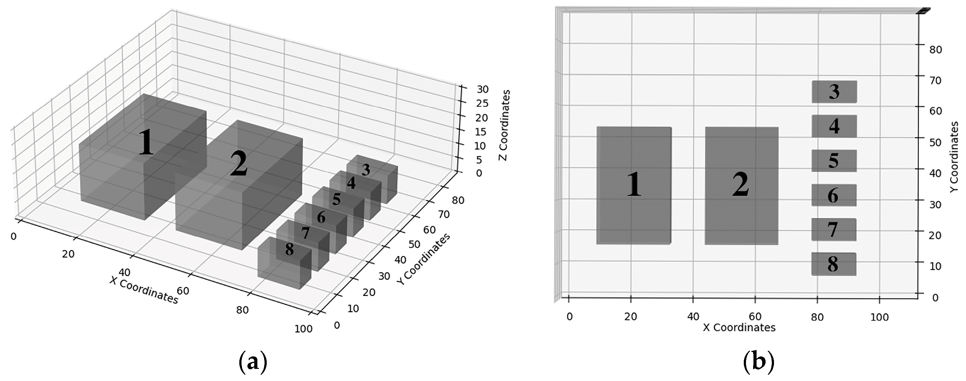
| Obstacle Number | Obstacle Coordinates | Equipment Name |
|---|---|---|
| 1 | Chiller 1 | |
| 2 | Chiller 2 | |
| 3 | Chilled water pumps 1 | |
| 4 | Chilled water pumps 2 | |
| 5 | Chilled water pumps 3 | |
| 6 | Cooling water pumps 1 | |
| 7 | Cooling water pumps 2 | |
| 8 | Cooling water pumps 3 |
| Name | Number of Units/ Units | Cooling Capacity/ kW | Evaporator Pressure Drop/ kPa | Condenser Pressure Drop/ kPa | |
|---|---|---|---|---|---|
| Original Program | Screw Chiller | 2 | 1737 | 87.5 | 77 |
| Optimized Program | Magnetic Levitation Chiller | 2 | 1759 | 46 | 35 |
| Name | Number of Individuals/ Individual | Drag Coefficient | Resistance/ kPa | |
|---|---|---|---|---|
| Original Program | Y-filter | 10 | 6.5 | 9.39 |
| Optimized Program | Cylindrical Filter | 10 | 5 | 5.06 |
| Original Program | Swing Check Valves | 6 | 2 | 2.89 |
| Optimized Program | Swashplate Check Valves | 6 | 0.45 | 0.65 |
| Parameter | Conventional | Optimized | Delta |
|---|---|---|---|
| 3,344,000 | 5,522,000 | +2,178,000 | |
| 600,320 | 313,958 | −286,362 | |
| 300,800 | 75,000 | −225,800 | |
| 334,400 | 552,200 | +217,800 | |
| 5 | 5 | 0 | |
| 10 | 10 | 0 | |
| 10,096,917 | 8,186,428 | −1,910,489 |
Disclaimer/Publisher’s Note: The statements, opinions and data contained in all publications are solely those of the individual author(s) and contributor(s) and not of MDPI and/or the editor(s). MDPI and/or the editor(s) disclaim responsibility for any injury to people or property resulting from any ideas, methods, instructions or products referred to in the content. |
© 2025 by the authors. Licensee MDPI, Basel, Switzerland. This article is an open access article distributed under the terms and conditions of the Creative Commons Attribution (CC BY) license (https://creativecommons.org/licenses/by/4.0/).
Share and Cite
Ma, X.; Cui, H.; Zhang, Y.; Wang, X. Study on Piping Layout Optimization for Chiller-Plant Rooms Using an Improved A* Algorithm and Building Information Modeling: A Case Study of a Shopping Mall in Qingdao. Buildings 2025, 15, 2275. https://doi.org/10.3390/buildings15132275
Ma X, Cui H, Zhang Y, Wang X. Study on Piping Layout Optimization for Chiller-Plant Rooms Using an Improved A* Algorithm and Building Information Modeling: A Case Study of a Shopping Mall in Qingdao. Buildings. 2025; 15(13):2275. https://doi.org/10.3390/buildings15132275
Chicago/Turabian StyleMa, Xiaoliang, Hongshe Cui, Yan Zhang, and Xinyao Wang. 2025. "Study on Piping Layout Optimization for Chiller-Plant Rooms Using an Improved A* Algorithm and Building Information Modeling: A Case Study of a Shopping Mall in Qingdao" Buildings 15, no. 13: 2275. https://doi.org/10.3390/buildings15132275
APA StyleMa, X., Cui, H., Zhang, Y., & Wang, X. (2025). Study on Piping Layout Optimization for Chiller-Plant Rooms Using an Improved A* Algorithm and Building Information Modeling: A Case Study of a Shopping Mall in Qingdao. Buildings, 15(13), 2275. https://doi.org/10.3390/buildings15132275