Finite Element Model Updating of Large-Span-Cable-Stayed Bridge Based on Response Surface

Abstract

Finite element (FE) model updating based on the response surface method using load test data of a cable-stayed bridge. This paper presents a case study of a cable-stayed bridge in which the FE model is refined using the response surface method based on experimental data from dead load and dynamic load tests. The elastic modulus and density of the main girder, tower, and cables are selected as the parameters to be updated, while the mid-span deflection and the first three vertical natural frequencies serve as the responses. The D-optimal experimental design is employed to generate test samples, and F-test analysis is performed to assess the significance of the parameters. The response surface equation is fitted using the least squares method, and the model’s accuracy is subsequently validated. The results show that the discrepancies between the FE model updating, and the experimental data are less than 3% for all responses, indicating a high degree of accuracy. This refined model demonstrates the effectiveness of the response surface method for improving the FE representation of the bridge. It can be applied in the field of damage detection, offering considerable practical value for bridge health monitoring.

1. Introduction

When creating an FE model, some simplifications can introduce computational errors. Additionally, field construction conditions, actual material properties, and noise can affect test data, causing discrepancies between the FE model results and the actual bridge structure test results, which do not meet the requirements for structural safety monitoring and evaluation technology research [1]. When studying the Qingzhou Cable-Stayed Bridge (with a main span of 605 m) on the Minjiang River in Fuzhou, China, it was found that the initial balanced configuration of the bridge has a significant impact on the FE calculations [2]. It is evident that updating the initial FE model to obtain an accurate benchmark FE model is essential. Depending on the different types of measured information, FE model updating methods can be divided into three categories: methods based on static test data, methods based on dynamic test data, and methods based on combined static-dynamic test data [3].The FE model updating method based on combined static and dynamic test data can avoid the shortcomings of separate static or dynamic tests, utilize more comprehensive information, and achieve better updating results [4].

Depending on the method used to adjust parameters, the FE model updating methods include the response surface method and the sensitivity matrix method. An FE model updating method based on multiple response surface data has been proposed, and its benchmark model has been applied to the field of damage identification [5]. An FE model updating method for civil engineering structures’ dynamics based on response surfaces has been proposed. And the main technologies for implementing updating methods have also been discussed [6]. The improved response surface method combining second-order polynomials with radial basis functions has been applied to the FE model updating of a tied-arch bridge, making the corrected FE model of the tied-arch bridge more consistent with the actual structure [7]. Deflection, strain, and frequency were selected as the response of Tongshan Bridge, which was corrected based on the response surface method, and the updating results were more favorable [8]. Based on the response surface and sparrow search algorithm, the model of a cantilever beam is revised. After revision, the errors in the first five natural frequencies of the bridge are all within 1% [9]. A steel-tube concrete composite truss bridge uses a central composite design for experimental design and fits a response surface. The revised model has high precision [10]. The above studies all use the response surface method for FE model updating, achieving good results. However, most of the bridge types targeted are medium- and small-span girder bridges, and the FE model updating methods used are mostly based on dynamic testing. A benchmark model establishment method based on ambient vibration measurement was proposed and validated in the Minjiang-Qingzhou cable-stayed bridge in Fuzhou, China [11]. The study focuses on large-span cable-stayed bridges, and the FE model updating method employed is based on dynamic testing methods. Thus, the model updating method that integrates both static and dynamic data can utilize more comprehensive information, effectively capturing the static and dynamic characteristics of the structure, resulting in improved updating outcomes. The FE model updating based on the response surface method overcomes the limitations of traditional model updating approaches. It offers the advantages of simplicity in computation, fast convergence speed, and high computational accuracy, making it more suitable for application in engineering practice. This paper employs the response surface method and integrates static-dynamic test data to refine the initial FE model of a large-span cable-stayed bridge. The goal is to achieve a more precise FE model to support the safety monitoring and evaluation of bridge structures.

2. FE Model Updating Using the Response Surface Method

Response surface method is a statistical approach based on experimental design, combining mathematical theory and statistical methods to deal with the transformation relationship between input variables and output responses in a system. Because the response surface model can replace the FE model for more effective calculations, it is also known as a model of models [10]. The steps for FE model updating based on the response surface method include selection of characteristic values; experimental design; parameter significance testing; fitting the response surface and precision testing; and optimization solution.

2.1. Experimental Design

Experimental design methods mainly include orthogonal design, D-optimal design, uniform design, and central composite design. Among these, D-optimal design not only significantly reduces the error of the response surface model but also requires fewer experimental samples with good fitting results. Therefore, this paper adopts the D-optimal design to obtain the sample.

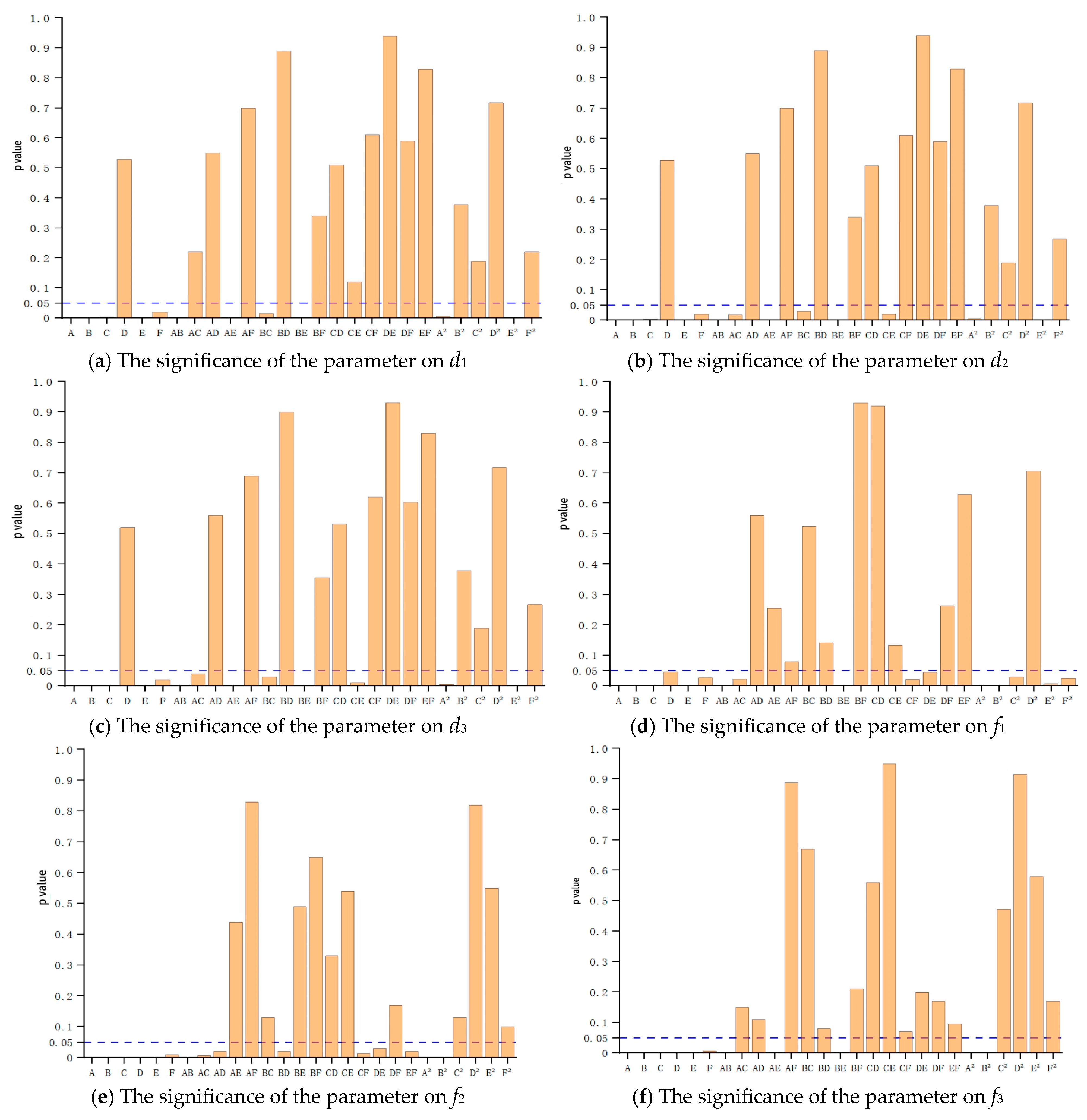
2.2. Parameter Significance Test

Since the selected updating parameters may not all have significant effects on the response, it is necessary to conduct a significance test to eliminate parameters that are not sensitive to the response. The criterion for screening updating parameters using the F-test is:

$$F_A={\displaystyle \frac{S{S}_A/f_A}{S{S}_e/f_e}}~F(J_A,J_e)$$

(1)

where:

• $S{S}_e$ —Sum of squares of deviations caused by experimental error.
• $S{S}_A$—Sum of squares of deviations caused by individual factors.
• $f_A$—Degrees of freedom for factors.
• $f_e$—Degrees of freedom for deviation.
• $F_A\ge F_{I-0.05}(f_A,f_e)$, $P\le 0.05$, the impact of the updated parameter A on the response is significant,
• $F_A\le F_{1-0.05}(f_A,f_e)$, $P>0.05$, the effect of the updated parameter A on the response is not significant, so it is excluded.

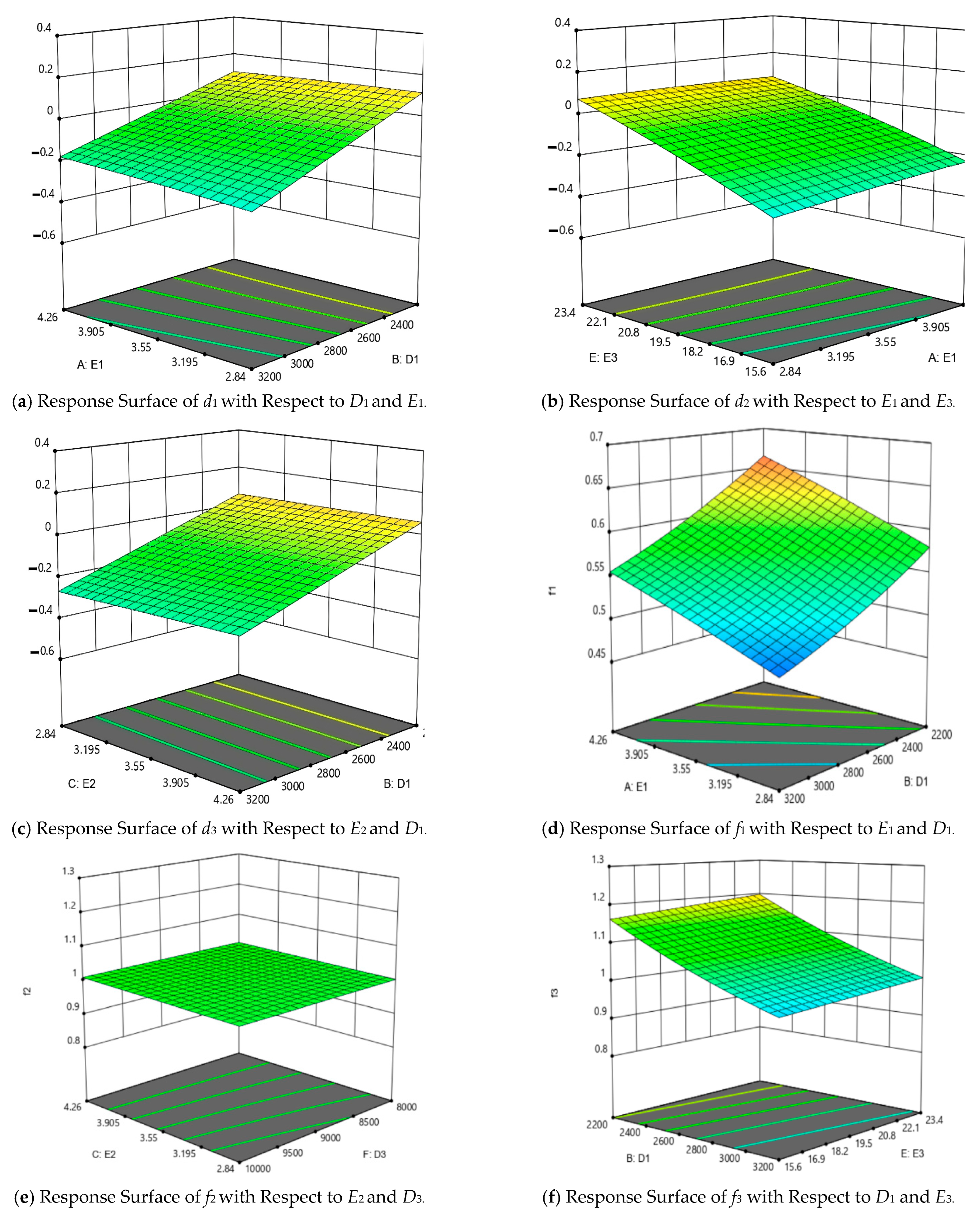
2.3. Fitting the Response Surface and Precision Check

Based on the characteristics of the FE model updating, a quadratic polynomial response surface model is adopted.

$$y={\beta }_0+{\displaystyle \sum _{i=1}^k{\beta }_i{x}_i+{\displaystyle \sum _{i=1}^k{\displaystyle \sum _{j=1}^k{\beta }_{ij}{x}_i{x}_j+{\displaystyle \sum _{i=1}^k{\beta }_{ii}{x}_i^2}}}}$$

(2)

Here, $x_i\in [x_i^l,x_i^n]$, $x_i^l$, $x_i^n$ are the lower and upper bounds of the values of the updated parameter x, respectively, ${\beta }_0$, ${\beta }_i$, ${\beta }_{\mathrm{ii}}$, ${\beta }_{\mathrm{ij}}$ are the regression coefficients.

After the fitting is completed, the accuracy is evaluated based on the $R^2$, $R_{\mathrm{adj}}^2$, $R_{\mathrm{pred}}^2$, respectively.

$$R^2=1-{\displaystyle \frac{S{S}_E}{S{S}_T}}(0\le R^2\le 1)$$

(3)

$$R_{adj}^2=1-{\displaystyle \frac{S{S}_E/d_E}{S{S}_T/d_T}}=1-{\displaystyle \frac{d_T}{d_E}}(1-R^2)(0\le R_{adj}^2\le 1)$$

(4)

$$R_{pred}^2=1-{\displaystyle \frac{PRESS}{S{S}_T}}(0\le R_{pred}^2\le 1)$$

(5)

where

• $S{S}_T\sqrt{a^2+b^2}$—total variance, $S{S}_T=S{S}_E+S{S}_R$
• $S{S}_E$—sum of squared errors,
• $S{S}_R$—Regression sums of squares,
• $d_T$—Total degrees of freedom in the model,
• $PRESS$—Predicted Residual Sum of Squares

The closer $R^2$, $R_{\mathrm{adj}}^2$ and $R_{\mathrm{pred}}^2$ are to 1, the better the fit of the response surface model if the difference between $R_{\mathrm{adj}}^2$ and $R_{\mathrm{pred}}^2$ is less than 0.2, which indicates that the response surface model has sufficient signal and can be used to predict unseen data [11].

2.4. Optimization Solution

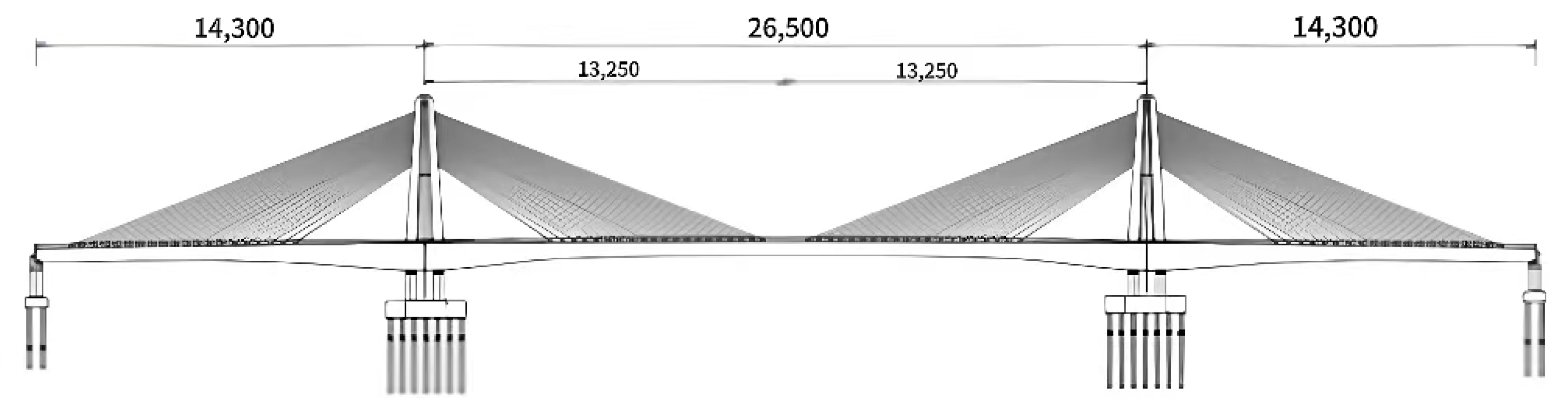
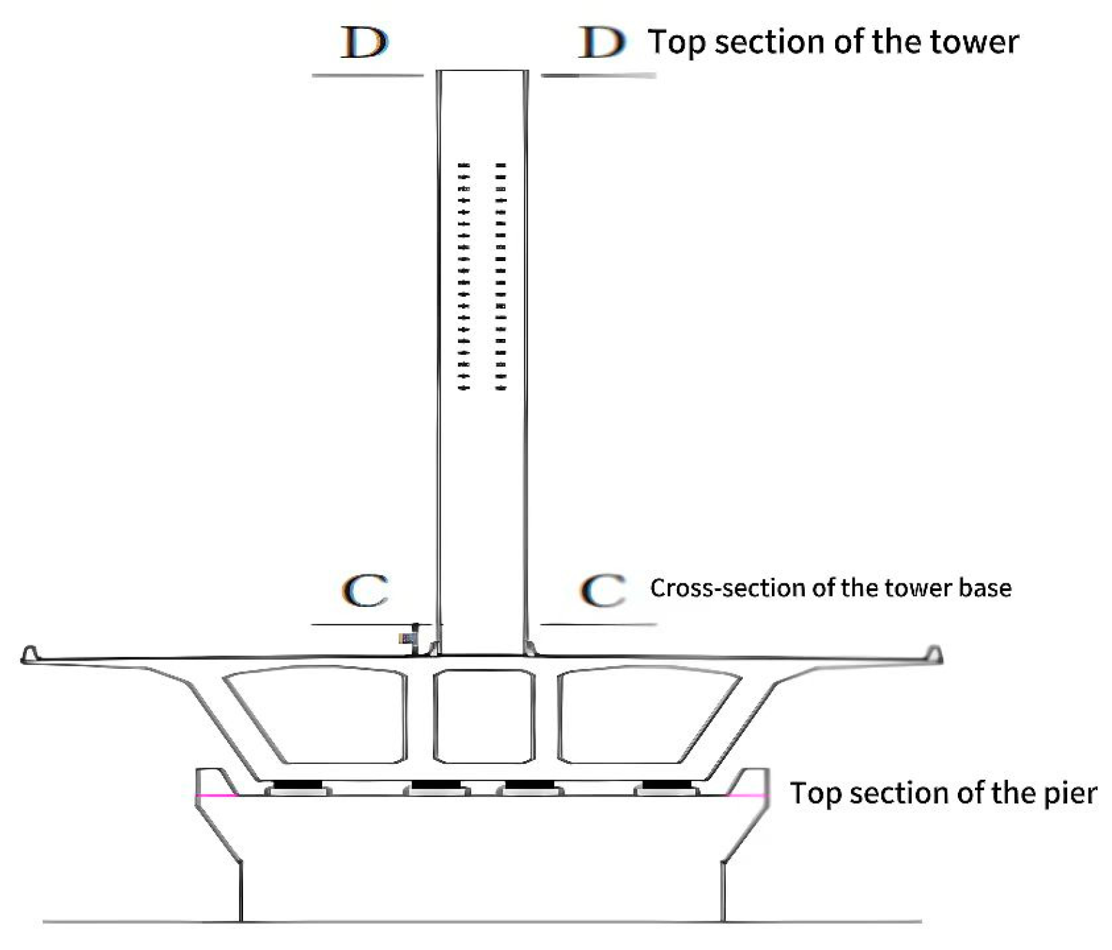
The problem of FE model updating can be formulated as the following optimization problem:

$$\left\{\begin{array}{c}Min\left(F\right(x)\\ lb\le x\le ub\end{array}\right.$$

(6)

In the equation, $F\left(x\right)$ is the objective function, $lb$ and $ub$ represent the lower and upper bounds of the updating parameters, respectively.

3. Project Overview

The overall layout of the Shang Deng Expressway South-to-North Water Diversion Special Bridge is shown in Figure 1. The superstructure adopts a double-tower single-cable-plane prestressed concrete short-tower cable-stayed bridge, with a structural system of tower-beam connection and pier-beam separation. The ratio of side span to middle span is 0.539. The main beam is a three-span prestressed concrete variable-section continuous box girder with spans of 143 m + 265 m + 143 m, designed for highway Class I load, with a design speed of 120 km/h and a secondary load of 162.6 kN/m.

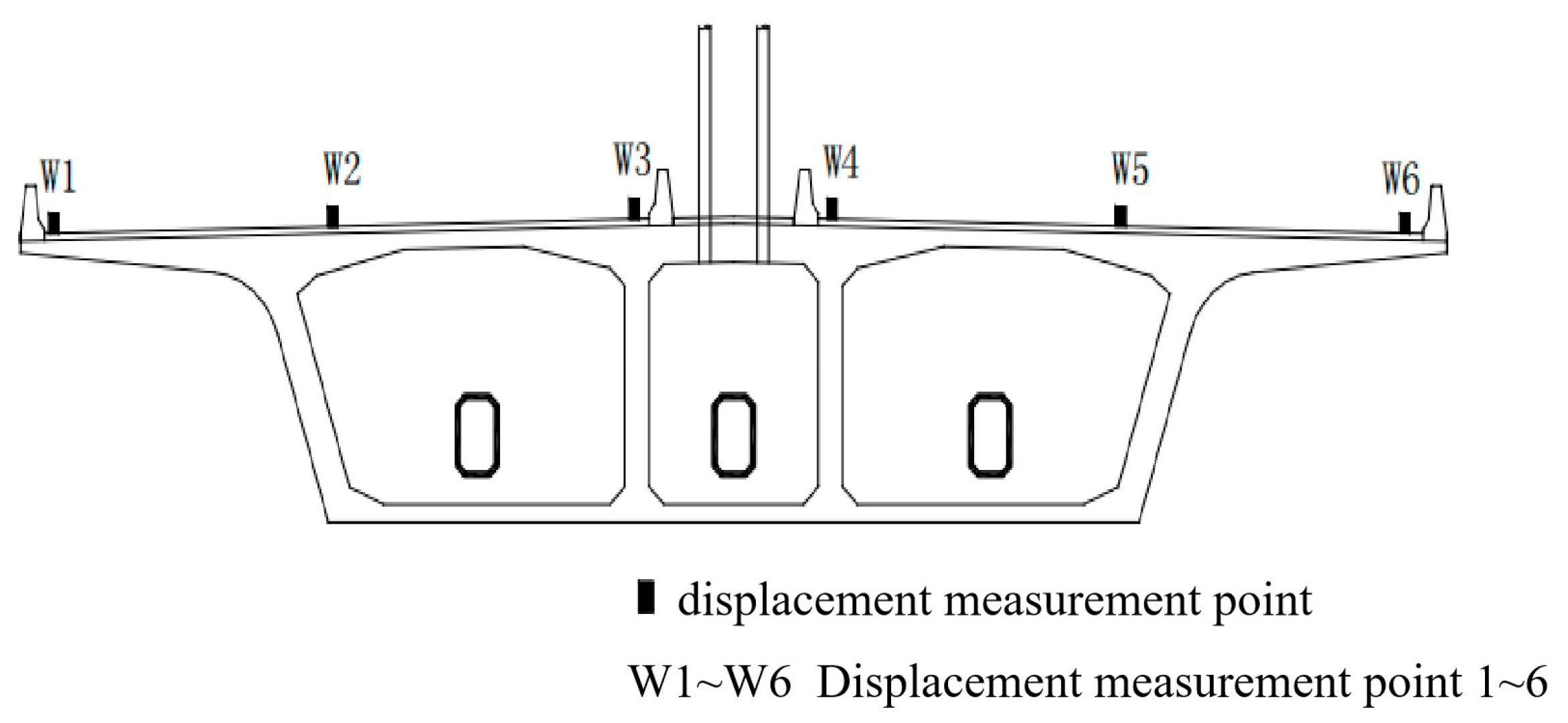
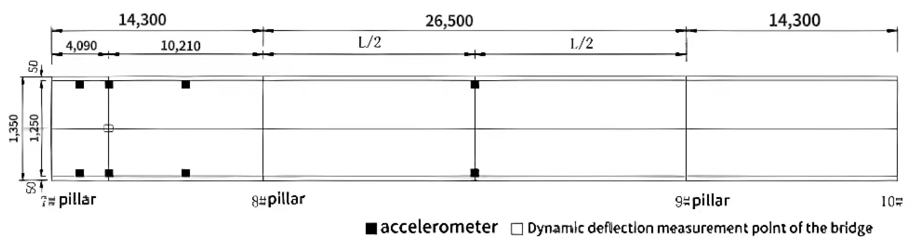
4. Static and Dynamic Load Testing

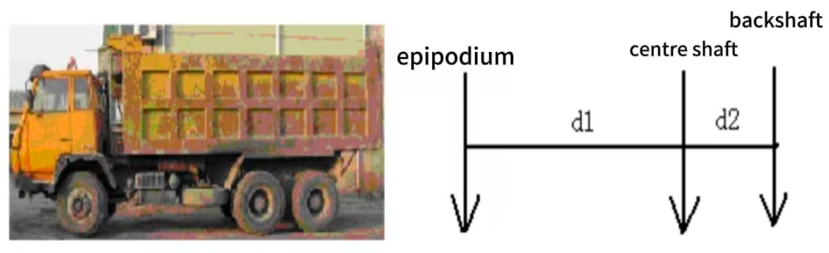
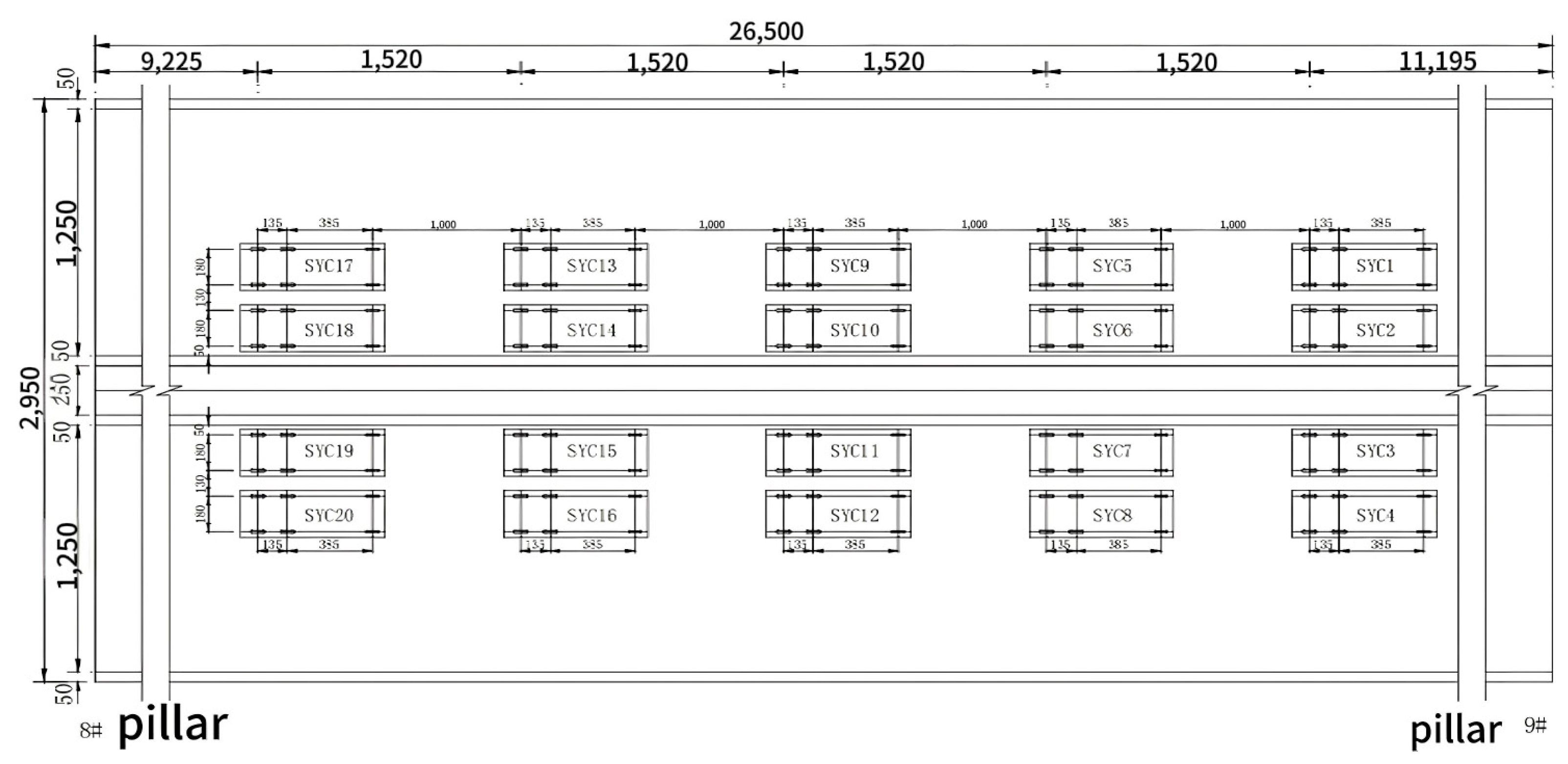
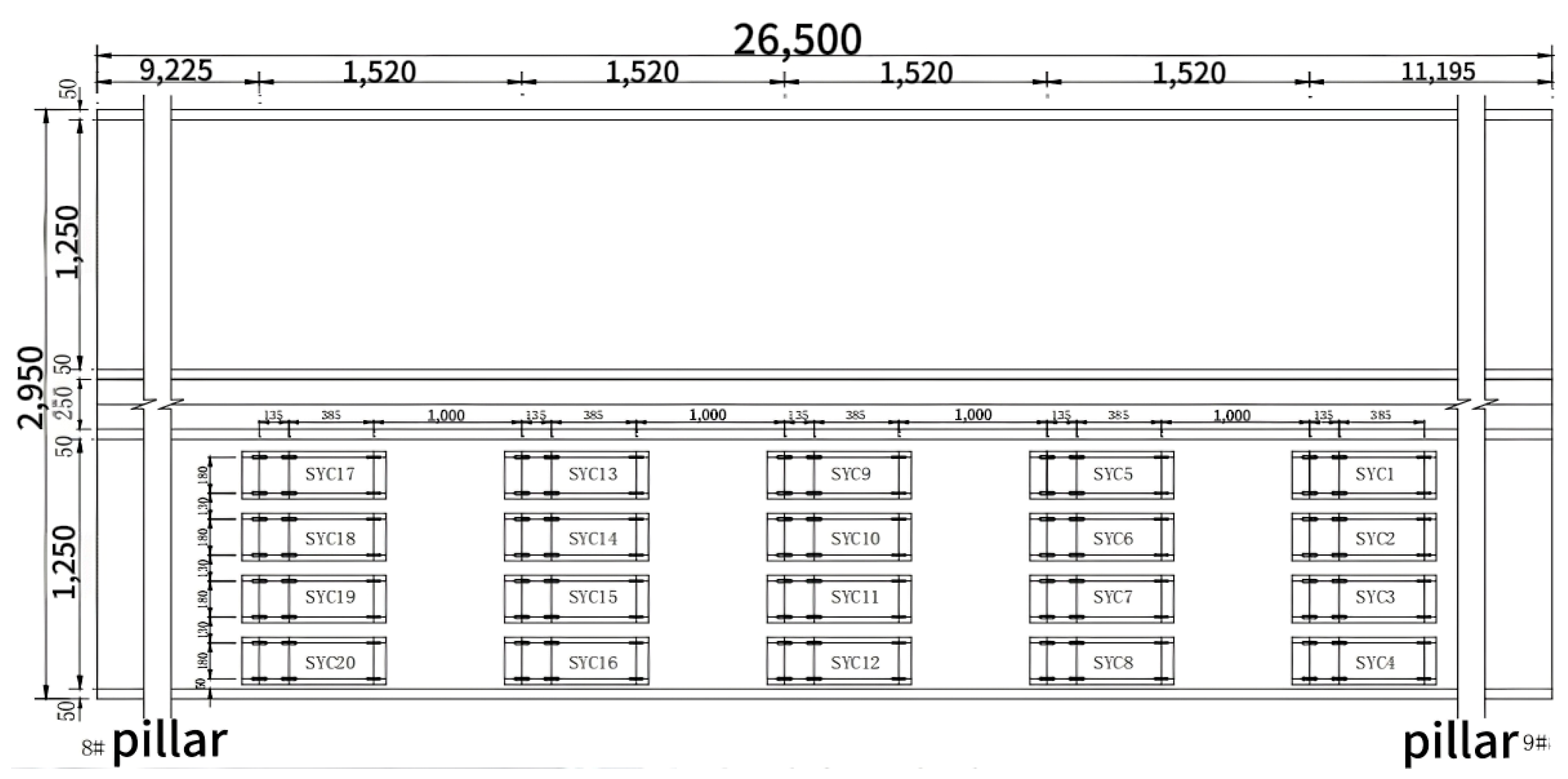
4.1. Static Load Testing

The static load testing was conducted using a dual-axle truck with a gravity load of 350 kN. The truck load was converted into three axle loads. The vehicle load model for the test is shown in Figure 2.

During the testing process, the test load was controlled by staged loading. The layout of the vehicle loading plane for some of the loads is shown in Figure 3 and Figure 4.

The maximum internal forces at the control section of the main girder, the maximum displacement of the main girder, the horizontal displacement at the top of the main tower, the maximum cable force of the stay cables, and the internal forces at the base section of the main tower were tested. Test sections mainly include the section with the maximum bending moment of the main girder, the section with the maximum negative bending moment of the main girder, the section with the maximum bending moment at the foot of the main tower, the section with the maximum longitudinal horizontal displacement at the top of the main tower, and the section with the maximum tensile force of the inclined cable at mid-span. The main girder test sections are shown in A-A and B-B in Figure 1, the main tower test section is shown in Figure 5, and the mid-span displacement measurement points are arranged as shown in Figure 6.

4.2. Dynamic Load Test

Choose a high-sensitivity, bidirectional, low-frequency velocity sensor with a frequency response range of 0.01 Hz to 100 Hz to obtain the first three vertical natural frequencies of the bridge. Six vertical velocity sensors are arranged at the edge spans, and two vertical velocity sensors are placed at the mid-span. One dynamic deflection measurement point is arranged at the middle of the bottom plate at the maximum positive bending moment of the edge span, as shown in Figure 7 (the edge span segment is 143 m, and the mid-span segment is 265 m).

5. FE Model Updating

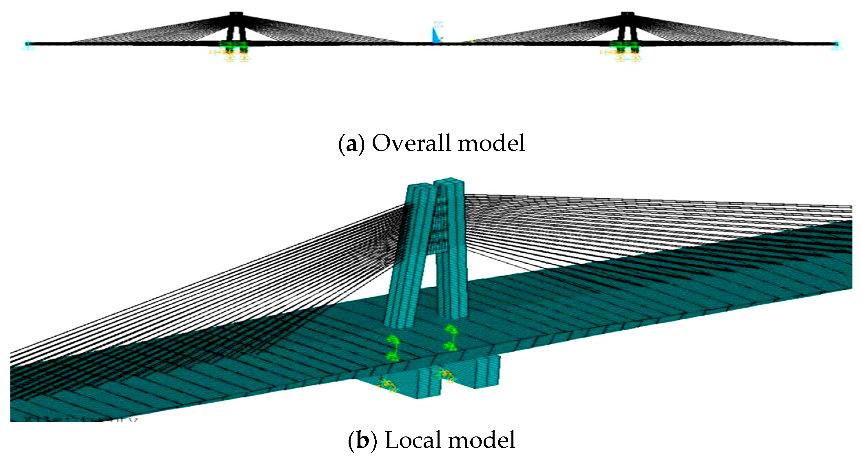
5.1. Initial FE Model

The full-bridge model was established using ANSYS 8.0 FE software, employing a tower-beam connection system. The main girder, bridge tower, and main pier were all modeled using Beam188 elements, the inclined cables were modeled using Link10 elements, and concentrated mass was modeled using Mass21 elements. The full-bridge model consists of 1487 elements and 1162 nodes. The main beam consists of a total of 149 elements, the main tower consists of 640 elements, the bridge pier consists of 68 elements, the stay cables consist of 160 elements, and the transverse beam consists of 320 elements. The modeling approach utilized a fishbone model, with the secondary load applied as a secondary mass uniformly distributed on the main girder. To ensure that the boundary conditions of the initial FE model are consistent with the actual bridge structure, the boundary conditions for each part of the structure were carefully defined during the establishment of the cable-stayed bridge model. The cable-stayed bridge adopts a structural system with tower-beam consolidation and pier-beam separation. Therefore, during the FE modeling, the base of the bridge pier is modeled with consolidation, restricting all its degrees of freedom. The bridge pier and main beam are simulated as supports using coupled nodes, while the main beam and main tower are consolidated and simulated using shared nodes. The full-bridge model is illustrated in Figure 8. The initial material properties of the model are listed in

Table 1. Material properties of the initial model.

	Material	Elastic Modulus/(×104 MPa)	Density (kg/m3)
Main beam	C60 Concrete	3.55	2600
Main tower	C60 Concrete	3.55	2600
Cable	Epoxy Coated Steel Strand	19.5	8500

.

The response measured in the static load test includes midspan deflection, maximum cable force of the cable-stayed bridge, and horizontal displacement at the top of the tower. The dynamic load test mainly measures the first three vertical frequencies of the structure. After comprehensive analysis, the midspan deflection and the first three vertical frequencies were chosen as the responses. After applying external loads equivalent to those in the static load test to the initial FE model, the midspan deflection and the first three vertical frequencies were calculated. The calculated values and measured values are shown in

Table 2. Calculated and measured response values.

	Deflection (cm)	First Vertical Natural Frequency (Hz)	Second Vertical Natural Frequency (Hz)	Third Vertical Natural Frequency (Hz)
Measured value	−5.5	0.586	1.074	1.172
Calculated value	−9.5	0.568	1.027	1.092
Error	72.7%	3.07%	4.38%	6.82%

.

As shown in Table 2, the midspan deflection of the FE model differs significantly from the actual cable-stayed bridge structure. The errors in the first two vertical frequencies are within 5%, while the error in the third vertical frequency is relatively larger. Therefore, the initial FE model has a significant deviation from the cable-stayed bridge, necessitating the FE model updating.

5.2. Selection of Eigenvalues

The main beam, tower, and cables of the cable-stayed bridge structure work together in coordination. The main beam bears most of the load, while the cables share part of the load, and the forces are transmitted to the foundation through the tower and piers. The elastic moduli of the main beam, tower, and cables are selected as parameters E₁, E₂, and E₃, and the densities of the main beam, tower, and cables are selected as parameters D₁, D_2, and D₃ to be updated. The deflections at the mid-span of the main span d₁, d₂ and d₃ and the first three vertical frequencies f₁, f₂, and f₃ under symmetrical load conditions at levels one, three, and five are taken as the responses. The variation range of the elastic moduli of the main beam, tower, and cables is set to ±20% of their initial values. The density range is determined based on engineering experience and several trial calculations, establishing a more reasonable parameter range as shown in

Table 3. Range of updating parameters.

Updating Parameters	Initial Value	Minimum Value	Maximum Value
$E_1$$(\times$104 MPa)	3.55	2.84	4.26
$D_1$ (kg/m3)	2600	2200	3200
$E_2$$(\times$104 MPa)	3.55	2.84	4.26
$D_2$ (kg/m3)	2600	2200	3200
$E_3$$(\times$104 MPa)	19.5	15.6	23.4
$D_3$ (kg/m3)	8500	8000	10,000

.

5.3. Experimental Design of the Case Study

The D-optimal experimental design is used to obtain the sample points, as shown in

Table 4. Experimental design samples.

Samples	${\mathit{E}}_1$$(\times$104 MPa)	${\mathit{D}}_1$ (kg/m3)	${\mathit{E}}_2$$(\times$104 MPa)	${\mathit{D}}_2$ (kg/m3)	${\mathit{E}}_3$$(\times$104 MPa)	${\mathit{D}}_3$ (kg/m3)
1	3.78	2395	2.84	2678.78	23.40	10,000
2	2.91	2200	3.01	2775	19.54	8860
3	2.88	2670	3.88	3030	18.06	10,000
4	3.48	3200	3.68	3200	19.62	8000
…	…	…	…	…	…	…
35	4.26	3062.84	3.05	2985	22.62	8980
36	3.75	2938.96	3.76	2770	18.56	9220
37	3.61	2200	4.26	2602.68	15.60	9550
38	2.84	3200	2.98	3200	15.60	9960

.

The sample points are substituted into the initial FE model to calculate the response values, as shown in

Table 5. Experimental design response values table.

Samples	${\mathit{d}}_1$ (m)	${\mathit{d}}_2$ (m)	${\mathit{d}}_3$ (m)	${\mathit{f}}_1$ (Hz)	${\mathit{f}}_2$ (Hz)	${\mathit{f}}_3$ (Hz)
1	0.18907	0.16116	0.13952	0.62072	1.0929	1.1773
2	0.11761	0.08285	0.05601	0.58204	1.0148	1.0913
3	−0.12124	−0.15648	−0.18369	0.52696	0.9235	0.98392
4	−0.20253	−0.23294	−0.25652	0.51821	0.91904	0.97834
…	…	…	…	…	…	…
35	−0.02534	−0.05112	−0.07120	0.57408	1.0243	1.0934
36	−0.15755	−0.18678	−0.20953	0.55163	0.9894	1.0462
37	−0.05346	−0.08451	−0.10871	0.61601	1.1173	1.1727
38	−0.46964	−0.50687	−0.53575	0.46886	0.83386	0.88289

.

5.4. Parameter Significance Test of the Case Study

Parameter selection is performed based on the F-test method to determine whether the updated parameters significantly affect the response. The significance level is set to 0.05, and the p-values for significance are calculated, as shown in Figure 9. The horizontal axis in the figure represents the selected parameters, where A, B, C, D, and F represent the chosen parameters E₁, D₁, E₂, D₂, E₃, and D₃.

As shown in Figure 9, the parameters A, B, C, E, and F have a highly significant impact on the mid-span deflection and the first three vertical frequencies. Parameter D has a highly significant impact on the first three vertical frequencies but has no significant effect on the mid-span deflection. The quadratic term A² has a very significant impact on all six responses; term B² has a significant impact on the first three vertical frequencies but no significant effect on the mid-span deflection; terms C² and F² have a highly significant impact on the first vertical frequency but no significant effect on the other responses; term D² has no significant effect on any of the six responses; and term E² has a highly significant impact on the mid-span deflection and the first vertical frequency but no significant effect on the second and third vertical frequencies. The interaction term AC has a significant impact on the mid-span deflection and the first and second vertical frequencies under the third and fifth loading conditions. The interaction term AD has a highly significant effect only on the second vertical frequency, with no significant impact on other responses. For other interaction terms, their significance can be inferred based on the F-test. Based on the results of the parameter significance test, parameters that have no significant effect can be excluded, while those that have a significant effect should be retained. After eliminating the insignificant terms, the results of the parameter significance analysis are displayed in Figure 10.

5.5. Fitting and Accuracy Verification of the Response Surface

Through D-optimal experimental design and significance analysis, the regression method using the least squares method was applied to fit each response. The established response surface model is shown in Figure 11.

The accuracy of each response surface model was tested, as shown in

Table 6. Accuracy test values of each response surface model.

Response Surface Function	${\mathit{d}}_1$	${\mathit{d}}_2$	${\mathit{d}}_3$	${\mathit{f}}_1$	${\mathit{f}}_2$	${\mathit{f}}_3$
R-squared	0.9999	0.9999	0.9999	1.0	1.0	0.9999
Adj R-squared	0.9998	0.9998	0.9998	0.9999	0.9999	0.9999
Pred R-squared	0.9996	0.9996	0.9996	0.9998	0.9999	0.9999

. The results indicate that the values for responses $R^2$, $R_{\mathrm{adj}}^2$, and $R_{\mathrm{pred}}^2$ are all close to 1, demonstrating a very high fitting accuracy of the response surface models. The difference between $R_{\mathrm{adj}}^2$ and $R_{\mathrm{pred}}^2$ is less than 0.2, indicating that the signal from the response surface models is strong enough to predict the location data.

5.6. Response Surface Function

Using the obtained response surface equation, optimization is performed within the design range of the parameters to be updated, using the MATLAB Optimization Toolbox. The optimal solution of the objective function (i.e., the updating values) and the comparison with the initial values are shown in

Table 7. Comparison of optimized parameters.

Updated Parameter	Initial Value	Updated Value	Change Range
$E_1$$(\times$104 MPa)	3.55	4.26	20.0%
$D_1$ (kg/m3)	2600	2758.6	6.1%
$E_2$$(\times$104 MPa)	3.55	2.84	−20.0%
$D_2$ (kg/m3)	2600	3017.3	16.1%
$E_3$$(\times$104 MPa)	19.5	20.7	6.2%
$D_3$ (kg/m3)	8500	9854	15.9%

.

5.7. Result Verification

5.7.1. Static Response Verification

The updated values are substituted into the initial FE model for calculation. The calculated deflection at the mid-span of the main span and the measured values are shown in

Table 8. Comparison of updated response calculation values and measured values.

Symmetric Loading	Measured Values (mm)	Initial Values (mm)	Updated Values (mm)	Relative Error Before Updating (%)	Relative Error After Updating (%)
Level 1	−15.0	−11.7	−13.5	22.00	10.00
Level 2	−29.9	−25.9	−26.1	13.38	12.71
Level 3	−37.4	−44.9	−39.1	20.05	4.55
Level 4	−45.3	−58.0	−50.7	28.04	11.92
Level 5	−53.8	−68.3	−59.7	26.95	10.97

.

As shown in Table 8, except for the second-level loading, the relative error of the deflection values under all other loading conditions has decreased by more than half compared to before updating. Moreover, the maximum error between the updated deflection values and the measured values decreased from 28.04% to 12.71%, and the minimum error decreased from 13.38% to 4.55%. The relative errors are all controlled within 15%. Although the relative error in the deflection value has significantly decreased, there are remaining errors. This may be due to the fact that the study did not account for the updating of cable forces and boundary conditions.

5.7.2. Dynamic Response Verification

The comparison of the calculated values and measured values of the first three vertical natural frequencies before and after structural updating is shown in

Table 9. Comparison of the first three vertical natural frequencies.

Order	Initial Value (Hz)	Measured Value (Hz)	Updated Value (Hz)	Relative Error Before Updating (%)	Relative Error After Updating (%)
$f_1$	0.576	0.586	0.595	1.7	1.5
$f_2$	1.026	1.074	1.073	4.5	0.1
$f_3$	1.091	1.172	1.141	6.9	2.7

.

As can be seen from Table 9, the first three vertical frequencies of the updated model are close to the measured values, with errors controlled within 3%. The maximum error between the updated frequencies and the measured values decreased from 6.9% to 2.7%, and the minimum error decreased from 1.7% to 0.1%. Among them, the error for the second vertical frequency is only 0.1%.

6. Conclusions

This paper employs the response surface method and joint static-dynamic testing data to conduct initial FE model updating for a specific cable-stayed bridge. The elastic modulus and density of the main beam, bridge tower, and stay cables of the cable-stayed bridge are selected as the parameters to be updated. The mid-span deflection and the first three vertical frequencies are selected as the response variables. The D-optimal experimental design method is used to design the experimental samples, and the F-test method is applied for parameter significance analysis. Then, response surface fitting is conducted based on the sample data, and the response surface model is validated for accuracy. Finally, the objective function is constructed. Based on the optimal solution provided by the optimization algorithm, the modified benchmark FE model has been obtained. The following conclusions have been drawn:

(1)

The p-values for the elastic modulus and density of the main beam and main tower, as well as the elastic modulus of the cable, are all below 0.05, indicating that their impact on the response is significant. The p-value for the cable’s density is greater than 0.05, indicating that its impact on the corresponding response is not significant.

(2)

The updated FE model more closely resembles the actual cable-stayed bridge, with the relative error of the static response reduced by over 50% and the relative error of the dynamic response now within 3%. It is evident that the model updating based on the response surface method is effective.

(3)

The model updating method that utilizes the response surface method is effective. This approach can be applied to the FE model updating real bridge structures and utilized in subsequent tasks, including health monitoring and damage assessment.

References

1. Wu, Z.; Huang, B.; Fan, J.; Chen, H. Homotopy based stochastic finite element model updating with correlated static measurement data. Measurement 2023, 210, 112512. [Google Scholar] [CrossRef]
2. Ren, W.-X.; Peng, X.-L. Baseline finite element modeling of a large span cable-stayed bridge through field ambient vibration tests. Comput. Struct. 2005, 83, 536–550. [Google Scholar] [CrossRef]
3. Yi, J.; Lunhua, B.; Yuntao, J.; Junjin, L.; Dongmei, Y. Study of load Tests for long-span Continuous Rigid Frame Bridge. J. Build. Sci. Eng. 2017, 34, 105–111. [Google Scholar]
4. Gang, L. Research on Finite Element Method Updating for Beam Bridge Based on Static and Dynamic Response Surface. Master’s Thesis, Southwest Jiaotong University, Chengdu, China, 2018. [Google Scholar]
5. Han, Z.; Wang, H.; Shao, Z.; Fu, H.; Jiang, H.; Wang, W. Finite difference method–based calculation of gravity deformation curve for the large-span beam of heavy-duty vertical lathe. Adv. Mech. Eng. 2016, 8, 1687814016646072. [Google Scholar] [CrossRef]
6. Ren, W.-X.; Chen, H.-B. Finite element model updating in structural dynamics by using the response surface method. Eng. Struct. 2010, 32, 2455–2465. [Google Scholar] [CrossRef]
7. Zhou, Y. Research on Model Correction Method Based on Response Surface and Its Application in Damage Identification of Continuous Girder Bridge. Master’s Thesis, Sichuan Agricultural University, Yaan, China, 2020. [Google Scholar] [CrossRef]
8. Xu, Z.; Xin, J.; Tang, Q. Finite Element Model Updating Based on Response Surface Method and Sparrow Search Algorithm. Sci. Technol. Eng. 2021, 21, 9094–9101. [Google Scholar]
9. Ma, Y.; Liu, Y.; Liu, J. Multi-scale Finite Element Model Updating of CFST Composite Truss Bridge Based on Response Surface Method. J. China Highw. Transp. 2019, 32, 51–61. [Google Scholar] [CrossRef]
10. Lu, P.; Li, D.; Shi, Q.; Chen, Y. Prediction method of Static Load Test Results of Variable Section Bridge Based on Dynamic Load Test Data. J. China Highw. Transp. 2022, 35, 213–221. [Google Scholar] [CrossRef]
11. Ren, W.X.; Lin, Y.Q.; Peng, X.L. Field load tests and numerical analysis of Qingzhou cable-stayed bridge. J. Bridge Eng. 2007, 12, 261–270. [Google Scholar] [CrossRef]
Figure 1. Overall layout (unit: cm).
Buildings 15 02247 g001
Figure 2. Loaded vehicle and vehicle load model.
Buildings 15 02247 g002
Figure 3. Symmetric load application layout (unit: cm).
Buildings 15 02247 g003
Figure 4. Layout of the eccentric load loading plane (unit: cm).
Buildings 15 02247 g004
Figure 5. Schematic diagram of the main tower test section locations.
Buildings 15 02247 g005
Figure 6. Layout of displacement measurement points at the mid-span section.
Buildings 15 02247 g006
Figure 7. Layout of dynamic measurement points.
Buildings 15 02247 g007
Figure 8. Initial model of the cable-stayed bridge.
Buildings 15 02247 g008
Figure 9. Parameter significance analysis chart.
Buildings 15 02247 g009
Figure 10. Significance analysis results of the parameters after removal.
Buildings 15 02247 g010
Figure 11. Response surface model. The closer the color is to red, the higher the value; the closer it is to blue, the lower the value.
Buildings 15 02247 g011