Abstract
Manual geometric modeling of timber structures is time-intensive and error-prone, impeding efficient structural analysis. To overcome this limitation, this study develops an automated framework for the rapid generation of 3D geometric finite element (FE) models directly from LiDAR point clouds. The methodology first employs a region-growing algorithm for component segmentation. This is followed by the integration of geometric feature extraction techniques to robustly determine the position, orientation, boundaries, and dimensions of structural elements. The extracted geometric information is then output as an executable APDL (ANSYS Parametric Design Language) file for parametric geometric modeling, incorporating interfaces for customizing material and connection properties. The proposed framework accurately reconstructs geometries with high fidelity. It effectively addresses challenges arising from occlusions and incomplete point cloud data through boundary inference and contact relationship analysis. This approach demonstrates substantial promise for applications in both heritage conservation and modern timber engineering.
1. Introduction
Wood material has been widely used in the construction of various types of buildings and structures, such as residential buildings, temples, wooden towers, bridges, palaces, etc., before the advent of concrete and steel. The long construction history has left behind countless historical timber structure-based architectural cultural heritages worldwide [1,2,3]. Preserving these heritage structures necessitates rigorous conservation and maintenance to ensure structural safety. Similarly, analyzing the structural integrity of existing timber buildings is crucial for their adaptive reuse. Concurrently, driven by the global demand for sustainable, low-carbon construction, engineered wood products are experiencing a resurgence in modern building applications.
Finite element (FE) models are essential tools for structural health monitoring, seismic analysis, and safety assessment of timber structures [4,5]. These models can simulate structural behavior under various external and internal factors, enabling the prediction of potential damage and failure modes. Generally, 3D FE models can be manually generated from detailed design drawings [6,7,8]. The authors of [9] reported an integrated structural–architectural framework that enables automated optimized structural design based on architectural sketching by importing simplified models to the commercial software SAP2000. S. Boonstra et al. [10,11] proposed a design grammar that enables the automated generation of a structural FEM for a given building’s spatial design. However, complexity, variability, and frequently the absence of original drawings of timber structures make accurate model reconstruction difficult. Traditional methods relying on field measurements and manual drawings are not only time-consuming and labor-intensive but also prone to errors. The limitations of these methods have highlighted the critical need for more efficient, reliable, and automated approaches to generating FE models.
The advent of advanced 3D laser scanning technologies offers a promising solution. Terrestrial laser scanners can efficiently capture high-density point clouds of structures, providing rich geometric data for modeling. Bouzas et al. [12] utilized point cloud data to assist historical drawings in determining the positions and arrangements of original, replaced, and reinforced components, thereby creating a 3D model of a steel bridge. Mol et al. [13] employed terrestrial laser scanners to collect point clouds from timber historical buildings spanning different periods and subsequently created a 3D HBIM (Historic Building Information Model) using BIM software. Beam components were generated using both manual segmentation and automated modeling techniques, and CloudCompare software was used to compare the point clouds of the beam components to assess structural geometric variations. Yang et al. [14] applied a semi-automatic method for manually segmenting steel bridge components and developed algorithms to automatically extract geometric information and create parametric BIMs. Romero-Jarén et al. [15] proposed an automatic method for segmentation, classification, and point cloud modeling to generate 3D surfaces of building elements, including floors, ceilings, walls, and columns; however, these 3D surfaces were not converted into corresponding three-dimensional building model elements. Zhang et al. [16] automatically generated a finite element model of a damaged reinforced concrete (RC) beam using 3D point clouds and 2D images, though the approach was limited to individual beam components. However, a fully automated pipeline for transforming raw point cloud data into complete geometric FE models of timber structures remains an unmet challenge. Ideally, this process should automatically encompass component segmentation, geometric feature extraction, and FE model generation.
Point cloud segmentation of structural components is a critical step in the automated generation of finite element models. The primary goal is to partition the point cloud data into distinct parts, each corresponding to an independent structural component. Common algorithms for point cloud segmentation include Hough Transform, Random Sample Consensus (RANSAC), Principal Component Analysis (PCA), Fast Point Feature Histograms (FPFH), region growing, Connected Components, Graph Cut, and Supervoxelization, among others [17]. Segmentation methods in structural engineering can generally be categorized into two types: those based on manually created models, which focus on specific structural features, and those based on data-driven models. Lu et al. [18] employed a slicing algorithm to classify bridge components, incorporating special component features such as relative length and surface normals during the evaluation process. Hamid-Lakzaeian [19] applied a multi-plane algorithm to classify building components in architectural facades. In recent years, significant advancements have been made in point cloud segmentation using deep learning techniques. Notable methods that directly operate on point clouds include PointNet [20], PointNet++ [21], and PointCNN [22]. Lee et al. [23] proposed HGCNN (Hierarchical DGCNN) for semantic segmentation of electric pole railway bridges, building on the concepts of PointNet and DGCNN (Dynamic Graph Convolutional Neural Network). Kim et al. [24] introduced a subspace partitioning method to enhance the prediction accuracy of the PointNet model for point clouds and performed longitudinal slicing of scanned bridge data to eliminate background noise. However, deep learning-based approaches typically require large volumes of labeled training data and significant computational resources, making them time-consuming and data-intensive. Robust segmentation methods suitable for the intricate geometries and frequent occlusions encountered in timber structures are still needed.
Extracting the geometric information of the target object from the point cloud is essential for generating a parametric finite element model. Yang et al. [14] proposed an algorithm that combines PCA with cross-section fitting techniques to extract the shape and orientation of circular bridge components from point clouds. They also developed an image-assisted edge point extraction algorithm to delineate the boundaries of planar structural components. Arayici et al. [25] investigated the feasibility of applying the point cloud obtained by a 3D laser scanner to generate a 3D CAD model and building information model (BIM) to represent the intensive architectural details of a historical building. A state of research of converting the raw point cloud into a semantically rich BIM is summarized in the literature [26]. Arias et al. [27] conducted FE analysis of a masonry arch bridge based on the geometric shape obtained from computer vision-based measurements. Lu et al. [28] employed a slicing strategy, first generating 3D shapes using the IFC (Industry Foundation Classes) data format and then fitting these shapes to labeled clusters of bridge point clouds. Kassotakis et al. [29] directly generated voxels from masonry structure point clouds for finite element simulation, representing the model as a sum of rectangular blocks connected by zero-thickness interfaces. This method, however, requires high integrity of the point cloud data. Generally, the geometry of structural members can be automatically estimated through feature point and edge extraction of point cloud data obtained by laser scanners or images [30,31,32,33]. However, a major persistent challenge is the incompleteness of point cloud data, especially for ancient timber structures where components are tightly interconnected, making complete scans difficult. Algorithms capable of accurately inferring geometric shapes and component boundaries from partial and occluded data are essential. The typical literature reports on point cloud modeling are summarized in Table 1. Current as-built modeling methods from cloud point data are mostly performed manually using software packages that may take several months depending on workers’ experience and the complexity of the facility.

Table 1.
Summary of typical literature reports on point cloud modeling.
To sum up, prior methods rely on manual intervention or partial automation (Table 1), especially for handling occlusions in complex timber joints. An end-to-end integration that fully automates segmentation, geometric reconstruction, and FE model generation for timber structures from raw point clouds is still massing. To address these critical gaps, this research proposes a novel, fast, and fully automated framework for generating geometric FE models of timber structures directly from 3D LiDAR point clouds. The main contribution lies specifically in integrating boundary inference and contact relationship analysis to overcome data incompleteness from occlusions and enable accurate reconstruction of hidden geometries. Based on this, a fully automated end-to-end workflow integrating region-growing segmentation, geometric feature extraction, and parametric APDL script generation—eliminating manual steps—can be provided. Section 2 introduces the acquisition and preprocessing of point cloud data, component segmentation, geometric information extraction, and the APDL modeling methods. Section 3 presents the validation and analysis of the geometric model through a case study. Section 4 concludes and discusses future work.
2. Methodology
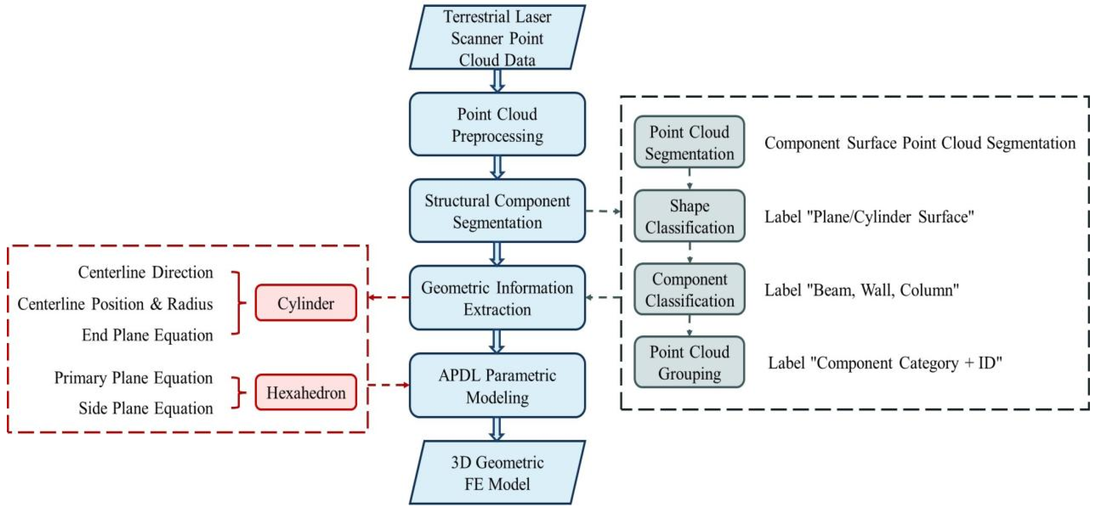
This section outlines the methodology employed for the automatic generation of geometric finite element (FE) models representing timber structures, starting from 3D point cloud data. The approach assumes that the input point clouds provide sufficient resolution. Figure 1 presents the overall process. First, raw point cloud data is collected through scanning equipment and then preprocessed through downsampling to ensure accuracy while maintaining processing efficiency. The consequent phase decomposes the preprocessed 3D point cloud representing the entire timber structure into its constituent structural elements. This segmentation identifies and isolates individual components such as beams, columns, walls, and other primary members. Then, algorithms are employed to extract precise geometric properties for each segmented component identified in the previous phase. Finally, the 3D geometric FE model is established by programmatically constructing APDL commands based on the extracted geometric properties. The detailed methods for each step are introduced in the following section.
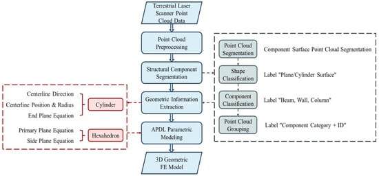
Figure 1.
Flowchart of the proposed method.
2.1. Raw Data Processing
Point cloud data were collected using a terrestrial laser scanner, with registration performed by software compatible with the Leica ScanStation P40. However, raw point cloud data are typically large, which increases the computational complexity. To improve processing efficiency, downsampling is applied to reduce point density while preserving essential information. Additionally, outliers are removed to enhance data quality, using the Open3D Python library.
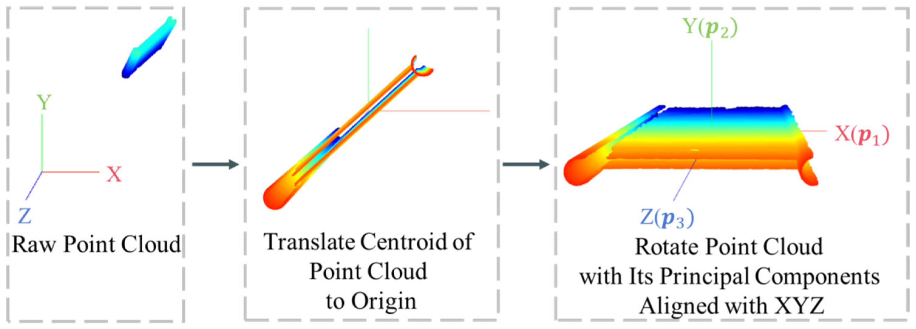
To establish a consistent reference frame for subsequent geometric computations, the raw data are referenced to an absolute coordinate system. To facilitate further calculations, a coordinate transformation is applied by computing the centroid of the point cloud and translating it to the origin . This alignment facilitates subsequent spatial analyses. PCA is then performed to determine the three principal components, , , and , which are aligned with the X, Y, and Z axes, as is shown in Figure 2.

Figure 2.
Coordinate transformation.
Let the point cloud be represented as , where . The mean vector is
The translation vector is
The translated coordinates are
Principal Component Analysis (PCA) decomposes point cloud covariance matrices to identify orthogonal axes of maximum variance [34]. PCA maps n-dimensional features to a k-dimensional space, where the k dimensions represent new orthogonal features, also known as principal components. These components are formed by projecting the original data onto the k-dimensional space. PCA identifies a set of orthogonal axes in the data, with each axis capturing the direction of maximum variance. The first axis captures the most variance, the second is orthogonal to the first, and the third is orthogonal to the first two, continuing until all n axes are determined.
The covariance matrix of the point cloud data is
The eigenvalues and eigenvectors of the covariance matrix are
The eigenvectors (principal components) are sorted in descending order according to their corresponding eigenvalues. These components, , , and , define a new coordinate system, with the rotation matrix:
The rotated coordinates in the new system are
In this process, the principal components capture the primary directions of variation. The Z-axis, representing one of these directions, is treated as a constant to reduce the impact of noise and missing data in the PCA calculation.
2.2. Component Segmentation
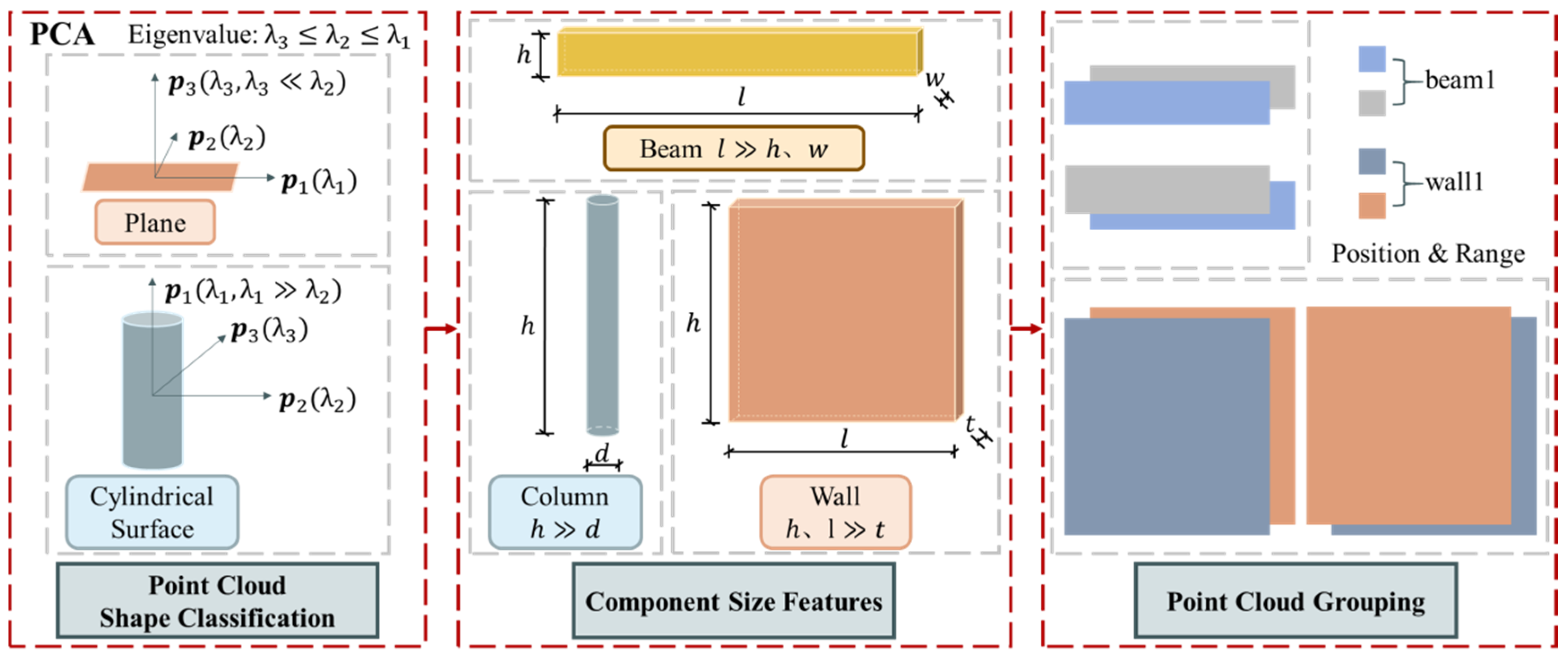
Segmentation partitions the point cloud into distinct structural components (e.g., beams, columns), enabling individualized geometric processing, as described in Figure 3. This study applies point cloud segmentation techniques to extract points corresponding to planes and cylindrical surfaces. Based on the shape and component categories of the segmented point clouds, labels are assigned to the regions. Finally, point clouds belonging to the same component are grouped and assigned a label representing an independent component.
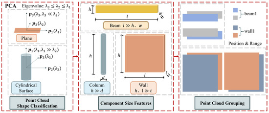
Figure 3.
The process of structural component segmentation.
2.2.1. Point Cloud Segmentation
Point cloud segmentation is the process of partitioning the point cloud based on spatial, geometric, and textural characteristics, ensuring that points within the same region exhibit similar features. The region-growing algorithm is applied to segment the cloud by grouping points with similar curvature and normal vectors. The algorithm involves the following steps:
(1) Set the minimum and maximum number of points in a cluster, denoted as and , respectively, as well as the smoothing threshold and the curvature threshold .
(2) Sort points by curvature and select the one with the smallest curvature as the initial seed point.
PCA is a widely used method for calculating normal vectors and neighborhood curvature. Calculate the eigenvalues of the covariance matrix and their corresponding eigenvectors ,,. The smallest eigenvalue corresponds to the normal vector of point , and the neighborhood curvature is computed as
Neighborhood curvature represents the local surface curvature around a point. A smaller value indicates a flatter surface, closer to a plane. After calculating the curvature for each point, the points are sorted, and the one with the smallest is chosen as the initial seed point.
(3) Initialize an empty sequence for the seed points and an empty cluster region . Add the selected initial seed point to the seed sequence and begin searching for neighboring points.
(4) For each neighboring point, compute the angle between the normal of the neighboring point and the normal of the current seed point. If is smaller than the smoothing threshold , the point is added to the cluster region .
(5) Examine the curvature of each neighboring point. If is smaller than the curvature threshold , add the point to the seed sequence .
(6) Remove the current seed point and continue the growth process using the newly added seed points. Repeat steps 3 to 5 until either the seed sequence is empty or the number of points in the remaining cluster falls below the minimum threshold .
This produces segmented clusters corresponding to candidate components.
2.2.2. Point Cloud Classification
After segmentation, further analysis is required to determine the specific shape features of the point cloud. Shape characteristics are inferred from the covariance eigenvalues, which provide information on the geometric structure of the cloud. On a plane, one eigenvalue is significantly smaller than the others, while on a cylindrical surface, one eigenvalue is much larger than the others [34], as illustrated in Figure 3. The eigenvalues are denoted as .
On a plane, the variation in one direction (typically the normal direction) is much smaller than in the other two directions, resulting in a relatively smaller corresponding eigenvalue. Consequently, the planarity is evaluated by the ratio of the second-largest eigenvalue to the smallest eigenvalue . If this ratio exceeds a threshold, the region is classified as a plane.
On a cylindrical surface, the variation in one direction (typically along the axis of the cylinder) is much greater than in the other two directions, resulting in a relatively larger corresponding eigenvalue. Consequently, the cylindrical surface is evaluated by the ratio of the largest eigenvalue to the second-largest eigenvalue . If this ratio exceeds a threshold, the region is classified as a cylindrical surface.
After classifying the point cloud based on its shape, the corresponding point cloud can be further processed through fitting. Following shape classification, component classification is also necessary to identify the actual structures corresponding to each segmented part, such as beams, walls, and columns. For this study, the focus is on the main structural components of a single-frame structure: beams, columns, and walls. The classification is based on the geometric characteristics of these components, as illustrated in Figure 3.
A beam is typically a long, slender structural element, with its length (along the cross-sectional direction) significantly greater than its width and height. A wall is a large planar structural element, with its height and length usually much greater than its thickness. A column is a vertical structural element, with its height (in the vertical direction) typically much greater than its diameter.
Point clouds are grouped according to component type, with each group labeled as ‘Component Category + ID’ (e.g., ‘beam1’, ‘wall1’).
2.2.3. Component Contact Relationship Determination
The point clouds corresponding to the contact areas between components are often difficult to capture, resulting in a loss of geometric information. To mitigate this, it is essential to determine the contact relationships between components and infer the geometric information of the contact areas. Here, neighboring distances and orientations between components infer contact relationships, which are crucial for boundary reconstruction. The specific judgment method is to traverse all points of all components and obtain the minimum distance between two points in the three directions of xyz. When the minimum value is less than the set threshold, it is considered that the two components are in contact.
2.3. Geometric Information Extraction
This stage extracts parametric geometries (e.g., centerlines, radii, planes) from segmented components, handling occlusions via inferred contacts.
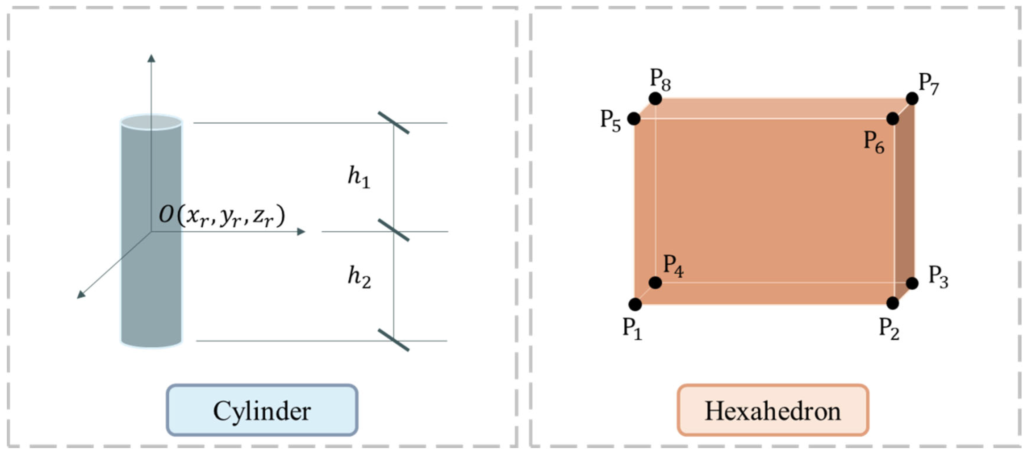
2.3.1. Cylinder
A cylinder is assumed to be a vertical component with its central axis aligned with the global Z-axis, represented by the direction vector (0, 0, 1). To simplify the 3D problem, the points are projected onto the XOY plane, reducing the task to two dimensions. The least squares method is then applied for circle fitting, which ensures accuracy even with sparse point cloud data.
Let the radius of the point cloud be denoted by , and the coordinates of the center by . The error function, based on the least squares principle, is given by
The partial derivatives of the error equation with respect to the parameters , , and are
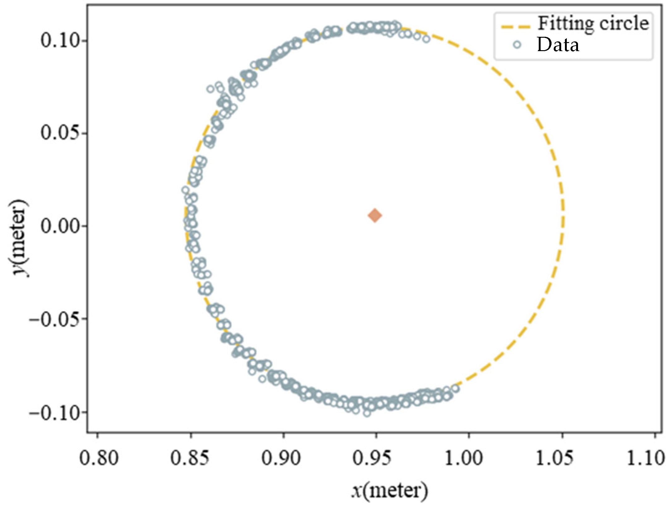
Solving these equations yields the parameters , , and that minimize the error function. The fitting diagram of a cylinder (e.g., wooden column) is shown in Figure 4.

Figure 4.
The fitting diagram of a cylinder.
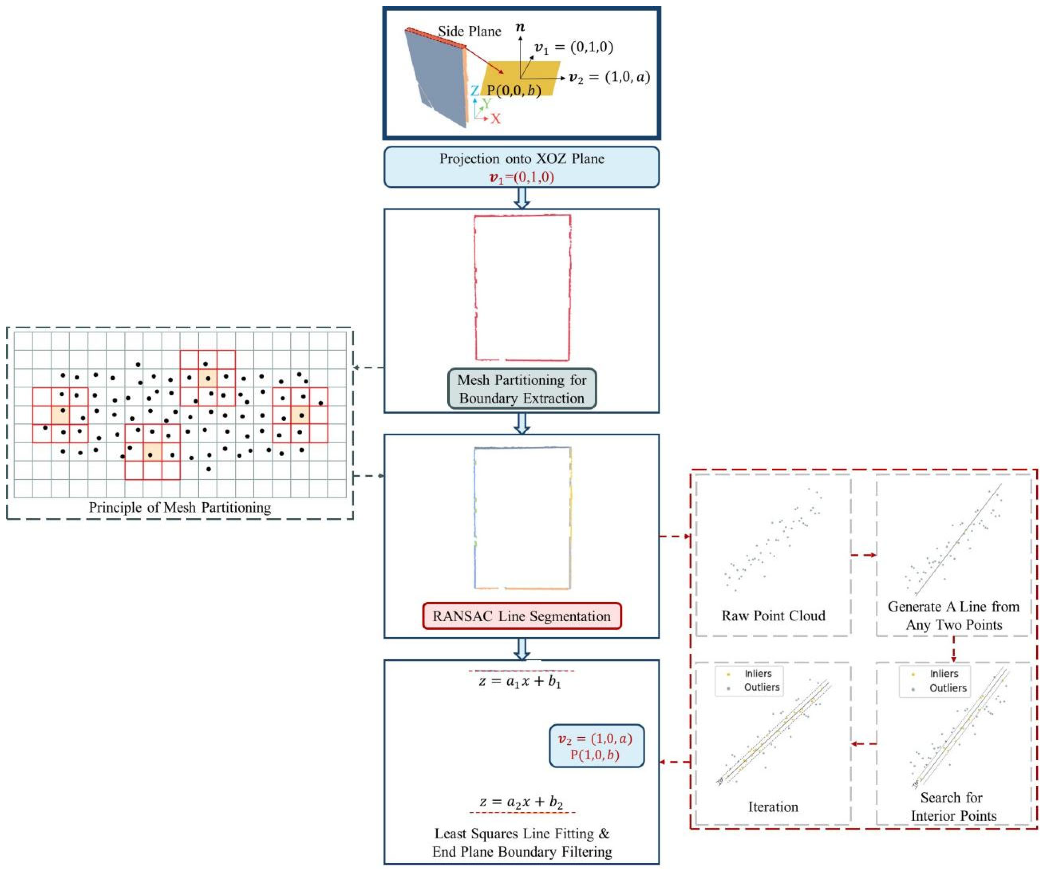
Due to structural occlusion, the point cloud of the cylindrical end plane cannot be directly scanned. However, the end plane parameters can be inferred by recognizing the boundary equation of the cylindrical surface point cloud. Losses at the top and bottom ends of the cylinder may hinder boundary recognition. To address this, boundary recognition utilizes the overall structure, with the top and bottom points on the cylindrical surface treated as the end plane’s boundary points. The point cloud is then projected onto a plane passing through the cylinder’s centerline, reducing the 3D problem to a 2D boundary recognition task. The normal vector of this projection plane becomes one of the direction vectors of the end plane.
Boundary points are first extracted using a mesh partitioning method, followed by point cloud line segmentation with the RANSAC algorithm. The least squares method is applied to derive the line equation parameters, allowing the end plane equation to be established. The whole process of end plane solving is shown in Figure 5.
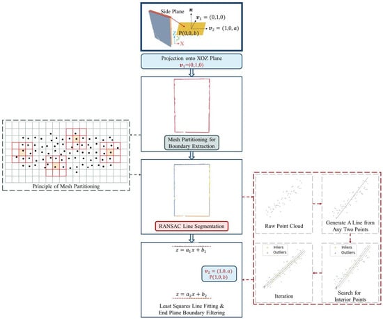
Figure 5.
End plane equation solving.
(1) Grid Division Method for Boundary Extraction
Inspired by edge detection in 2D images, the point cloud is divided into square grids to identify boundary points. The grid side length depends on the point cloud’s density and downsampling rate. The steps are as follows:
(i) Grid Division: The point cloud is projected onto the XOZ plane to obtain the 2D point cloud set q , where . First, traverse all points to obtain , , , , and construct the minimum bounding box of the point set.
The point cloud is projected onto the XOZ plane to obtain the 2D point cloud set q , where . The maximum and minimum values of x and z are determined to construct the point set’s minimum bounding box. The grid side length l is chosen based on point cloud density, and the number of grids in the X and Z directions is calculated as
The points are assigned to corresponding grid cells , where u and v. After assignment, grids are categorized into filled grids (containing data points) and empty grids.
(ii) Boundary Grid Identification: For each filled grid, the number of neighboring empty grids is checked. If at least one of the eight neighboring grids is empty, the current grid is classified as a boundary grid.
(iii) Extract Boundary Points: Boundary points from each identified grid are extracted for subsequent point cloud line segmentation.
(2) RANSAC Algorithm for Point Cloud Line Segmentation
RANSAC (Random Sample Consensus) is an iterative model estimation method that estimates the parameters of a mathematical model from a dataset containing outliers. The basic idea of RANSAC is to repeatedly select random subsets of data to estimate the model and compute the consistency of the model with the entire dataset. The specific steps are outlined below, with steps describing the point cloud fitting process.
- (i)
- Randomly select two points and solve for the line parameters they define.
- (ii)
- Calculate the distance from the remaining points to the line equation, and compare this distance with a preset threshold δ. If the distance is smaller than δ, classify the point as an inlier; otherwise, classify it as an outlier. Then, count the number of inliers.
- (iii)
- Repeat steps (i) and (ii). If the number of inliers for the current model exceeds the previously recorded maximum number of inliers, update the model parameters, retaining the model with the highest number of inliers.
- (iv)
- Iterate steps (i) to (iii) until the preset iteration threshold k is reached, finding the model parameters with the most inliers. Finally, use these inliers to re-estimate the model parameters and obtain the final model parameters.
- (v)
- Remove the inliers found from the original point cloud to form a new point cloud.
- (vi)
- Repeat steps (i) to (v) on the new point cloud until all lines are identified, as shown in Figure 5.
(3) Least Squares Fitting of the Line Equation and Boundary Filtering
The line equation of the segmented point cloud is solved using the least squares method. Let the line equation of the point cloud be . According to the least squares principle, the error equation is written as
The partial derivatives of the error equation with respect to parameters a and b are
By solving the equations where these partial derivatives are equal to zero, the parameter values a and b that minimize the error function can be found.
The parameter a represents the slope of the line, and since the end plane is approximately parallel to the horizontal ground, the slope of the relevant line boundary is close to zero. Using this condition, the line equations corresponding to the end plane are selected. By analyzing the parameter , the lines corresponding to and are determined to define the upper and lower boundaries, as shown in Figure 5.
(4) Calculating the End Pace Equation
The line boundary equations obtained earlier have the direction vector , where . Therefore, two non-parallel direction vectors for the end plane can be determined:
The normal vector of the end plane is
The equation of the plane is given by , and a point P lies on the plane. Thus, the coefficients are
From this, the equation of the end plane can be determined.
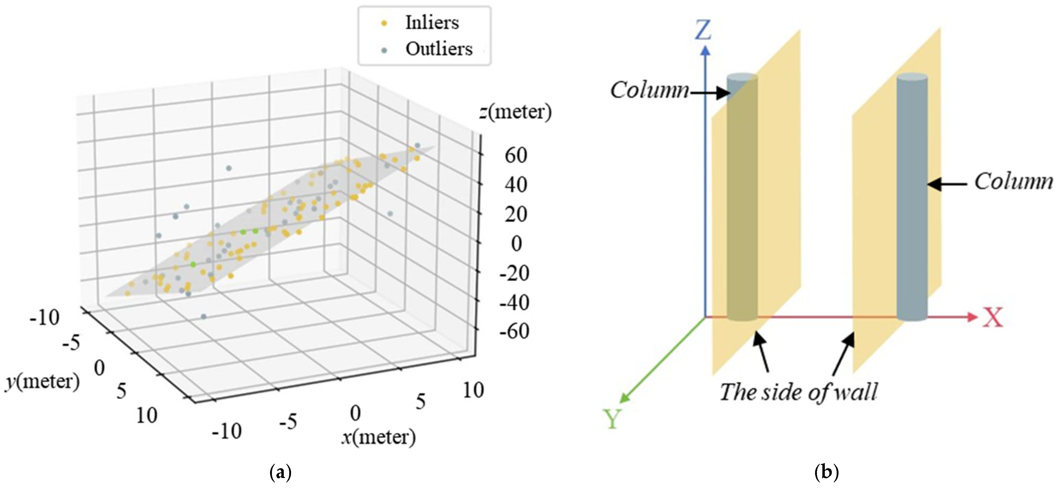
2.3.2. Hexahedron
Hexahedral components (e.g., beams/walls) require fitting six bounding planes. Due to the limited scanning range of the scanner and issues like occlusion of component contact surfaces, the point cloud primarily captures data from the front and rear primary planes. Consequently, the parametric equation of the primary plane can be directly obtained through point cloud fitting (as shown in Figure 6a). However, for the side planes, point clouds must be derived from the boundaries of the primary plane point cloud.
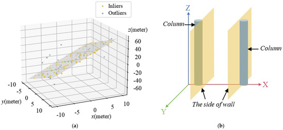
Figure 6.
The diagram of geometry information extraction: (a) RANSAC algorithm plane fitting; (b) side equations acquisition.
In this study, the RANSAC algorithm is used for plane fitting to determine the parametric equation of the primary plane. Three points are randomly selected from the dataset to define the plane model in the form . The distance of all other points from this plane is calculated as the model’s error. A threshold is set, classifying points with distances smaller than this threshold as inliers. If the number of inliers exceeds that of the previous model, the plane model is updated. This process iterates until the preset number of iterations is reached, or a satisfactory model is found. The procedure follows a similar approach to line fitting.
For side planes not in contact with a cylinder, the fitting process follows a method similar to that for cylindrical end planes. The point cloud of the primary plane is projected onto the XOZ plane to extract the boundary. For components in contact, such as beams and walls, the parametric equations of the side planes are obtained, averaged, and adjusted to ensure proper contact.
When the side plane does contact a cylinder, its parametric equation is derived from the cylinder’s equation, ensuring tangency(as shown in Figure 6b). After the coordinate transformation outlined in Section 2.1, the side plane is approximated as parallel to the YOZ plane. Using the cylinder’s central line direction, position, and radius, the equation of the side plane is then determined.
2.4. Automatic Generation of Geometric Finite Element Model
The extracted geometries are converted into an APDL script for parametric FE modeling in ANSYS 19.0. APDL is a parameterized design language for ANSYS that enables users to customize and automate their workflows through scripting. This study employs APDL (ANSYS Parameter Design Language) to automate parametric modeling of FE models. By processing the geometric and positional data from the point cloud, an APDL command file is generated to model the components parametrically, leading to the creation of a geometric FE model of the structure.
For cylindrical components, modeling occurs in their local coordinate system by first translating the coordinate system to the centerline and then inputting the radius and end plane height. For hexahedral components, modeling is performed by generating a solid from eight corner points. The APDL commands for different components are encapsulated in functions. These functions take the geometric parameters and positional data as inputs and output the corresponding APDL file, which is used in ANSYS to generate the FE model for subsequent structural analysis. The modeling process is shown in Figure 7.
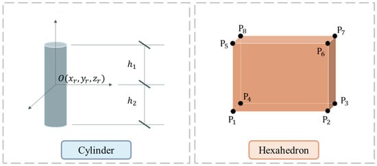
Figure 7.
The process of APDL parametric modeling.
3. Experiments and Discussion
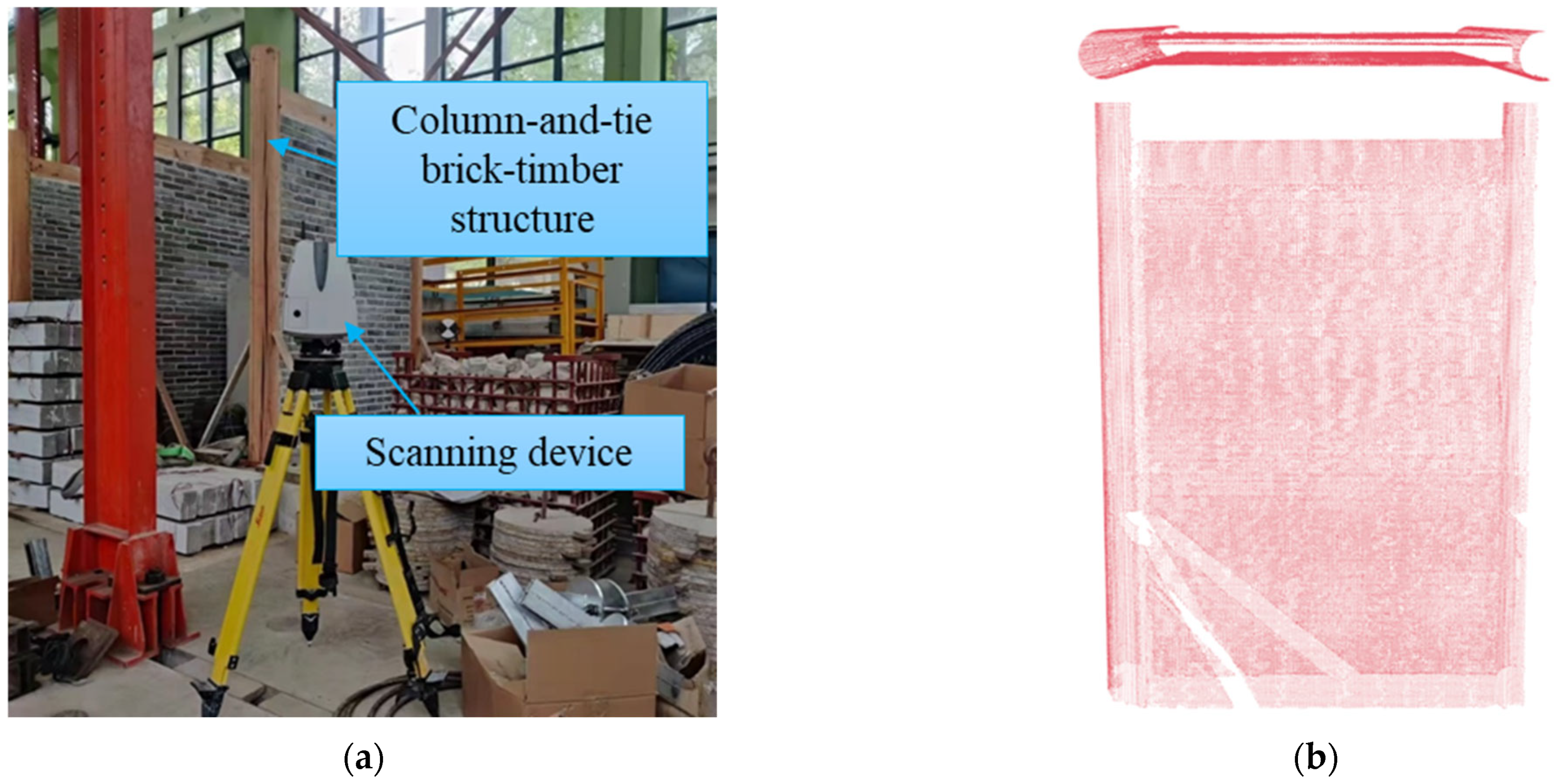
The methodology section presents a technique for quickly and automatically generating a FE model from point cloud data. To validate this method, a case study is conducted on a column-and-tie brick–timber structure.
3.1. Verification of Geometric Model
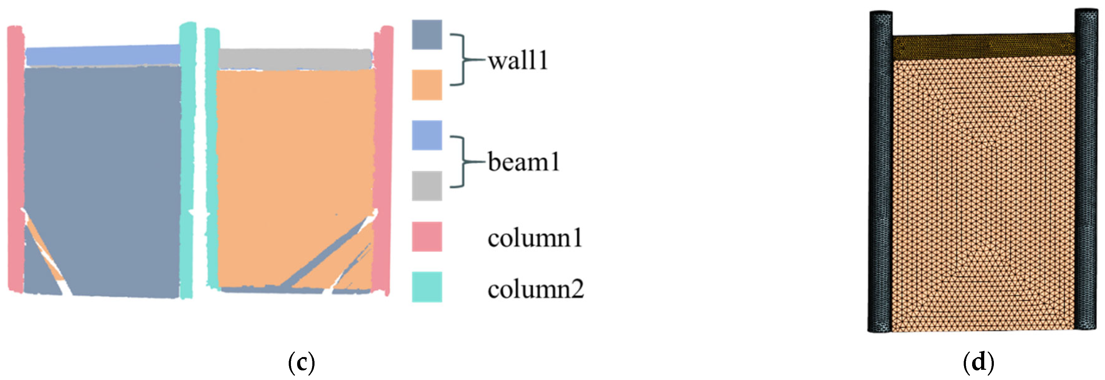
Point cloud data were collected using a Leica ScanStation P40 (perchased from Leica Geosystems AG, München, Germany), with an angular accuracy of 8″ and distance measurement accuracy of 1.2 mm ± 10 ppm. The data collection site is depicted in Figure 8a. Due to the relatively small size of the structure, two stations were used for actual scanning. The point cloud data acquired from both stations were registered and merged using Leica’s proprietary post-processing software. The original dataset consists of 114,854 points, which are downsampled globally to reduce computational burden and speed up processing, as shown in Figure 8b. The original scanning point cloud has low noise and high quality, which is conducive to geometric shape fitting and reduces the difficulty of parameter tuning.
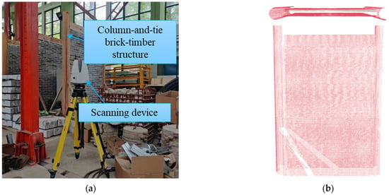
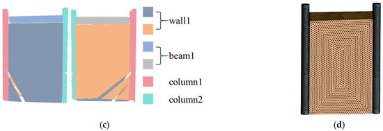
Figure 8.
Validation in the case study: (a) point cloud acquisition; (b) point cloud data; (c) structural component segmentation; (d) geometric FE model.
In the component segmentation process, the region-growing method is applied with smoothing and curvature thresholds of 6° and 0.01, respectively. A feature value ratio of 50 is used to classify the points as either plane or cylinder. Points are grouped by spatial range, and the structural component type is determined. The grouped point clouds are then labeled, as shown in Figure 5.
For point cloud fitting, RANSAC is used for plane fitting with a distance threshold of 0.003 m, and line fitting is performed with a threshold of 0.015 m. Boundary extraction is carried out using a mesh partition method with a grid size of 0.02 m. All key parameters utilized in the proposed method are summarized in Table 2. The selection of parameters would critically influence both geometric accuracy and computational efficiency in the proposed framework. For region-growing segmentation, increasing the smoothing threshold reduces computational burden but risks over-segmentation by merging distinct components with divergent normals. Conversely, stricter thresholds improve boundary precision at the cost of increased iteration time. Similarly, a higher curvature threshold accelerates processing but may misclassify cylindrical surfaces as planar, while lower values enhance shape differentiation at computational expense. In RANSAC-based geometric extraction, enlarging the plane fitting distance tolerance improves convergence speed but introduces surface parameter deviations by incorporating outliers, whereas tighter tolerances yield more accurate plane orientations despite longer processing. The same trade-off applies to line fitting tolerance, where higher values expedite boundary detection but compromise end-plane reconstruction accuracy. For boundary extraction via grid partitioning, larger grid sizes significantly accelerate processing but fail to capture fine edges, while smaller grids improve boundary completeness at a quadratic computational cost.
Table 2.
Key parameters in the proposed framework.
To sum up, increasing any tolerance threshold enhances efficiency but reduces geometric fidelity. The case-specific optimal values (Table 2) balance these competing objectives, though performance remains sensitive to point cloud characteristics—higher noise or occlusion necessitates tolerance relaxation to maintain robustness, whereas clean data supports stricter settings for maximal accuracy.
Notably, the parameters in Table 2 were determined through experimental tuning. This tuning process incorporates a feedback mechanism to ensure parameter selection is both rational and optimal. Cylindrical components are characterized by fitting their centerline positions and radii using least squares, while their end-face planes are derived through mesh partition combined with RANSAC line fitting. The heights of the upper and lower end faces are subsequently determined by calculating their intersection points with the established centerline. Furthermore, parameter sensitivity was rigorously minimized during the tuning phase.
For hexahedral components, the primary plane equation is derived via RANSAC plane fitting, and side planes are obtained from the primary plane boundaries or the geometric information of contacting cylinders. Using these six plane equations, the eight corner points of the component are calculated, and the component is modeled using APDL point generation. Beam and column components have a mesh size of 20 mm, while wall components use a mesh size of 50 mm. The segmentation of all components is depicted in Figure 8c. The resulting APDL-based geometric FE model is shown in Figure 8d.
The case study was executed on a laptop with an 11th Gen Intel® Core™ i7-11800H CPU and Intel® UHD Graphics GPU. The time to generate the geometric model from the point cloud was approximately 9.75 s, demonstrating the method’s efficiency in reducing modeling time and workload. It is worth emphasizing that the efficiency of point cloud modeling is closely related to the complexity of the scanned object. Yang et al. [14] took about 60 min for manual segmentation of their scanner steel structures, then took about 180 min to extract geometry information for all components. One recent study also shows that even with skilled workers, the state-of-the-art software, and special care for time saving, 30 days were spent on the 3D BIM modeling of six commercial buildings from point cloud data [35]. Currently, these modeling methods are mostly performed manually using software packages that may take several months depending on workers’ experience and the complexity of the facility.
To assess the accuracy of the point cloud recognition for geometric shapes, the extracted geometric information was compared with the actual dimensions of the structure. For beam components, length, width, and height were compared; for wall components, length, thickness, and height were considered; and for cylindrical components, radius and height were examined (Table 3). The relative errors for all dimensions were within 3%. The tilt angles of the planes, except for the cylinder’s centerline and the plane in contact with the cylinder, are detailed in Table 4. The absolute angular errors between these planes and the horizontal or vertical planes were all within 1°, confirming that the proposed method achieves sufficient accuracy for structural modeling. Inevitable occlusion during data collection resulted in a partial point cloud missing in the tested wooden structure. Given the structural simplicity of the case study, a geometric feature-based completion technique was employed to address the missing data. However, such incompleteness in the scanned point clouds constitutes a potential source of error. Therefore, when applying this method, ensuring the integrity of the original scanned point cloud data is paramount.
Table 3.
Geometric dimensional accuracy evaluation.
Table 4.
Plane tilt assessment.
The results presented in Table 3 demonstrate that the proposed method achieves high accuracy in identifying simple geometric wooden components. Nevertheless, wooden structures exhibit diverse structural forms, with modern designs frequently incorporating geometrically complex prefabricated glued laminated timber components. The current approach relies primarily on manually defined parameters and rules, which inherently limits its capability to handle components with complex shapes. For instance, determining optimal segmentation strategies often necessitates manual threshold or rule specification, a process that becomes increasingly challenging with complex geometries.
3.2. Analysis of FE Model
Notably, the output of the proposed method is an executable script. The geometric finite element model was obtained by importing the script into the APDL platform. However, since complete finite element analysis requires additional input variables—such as material properties and load conditions—which are not acquired during static scanning, this study incorporates user-defined input interfaces for these parameters within the generated executable file. This facilitates subsequent comprehensive finite element analysis.
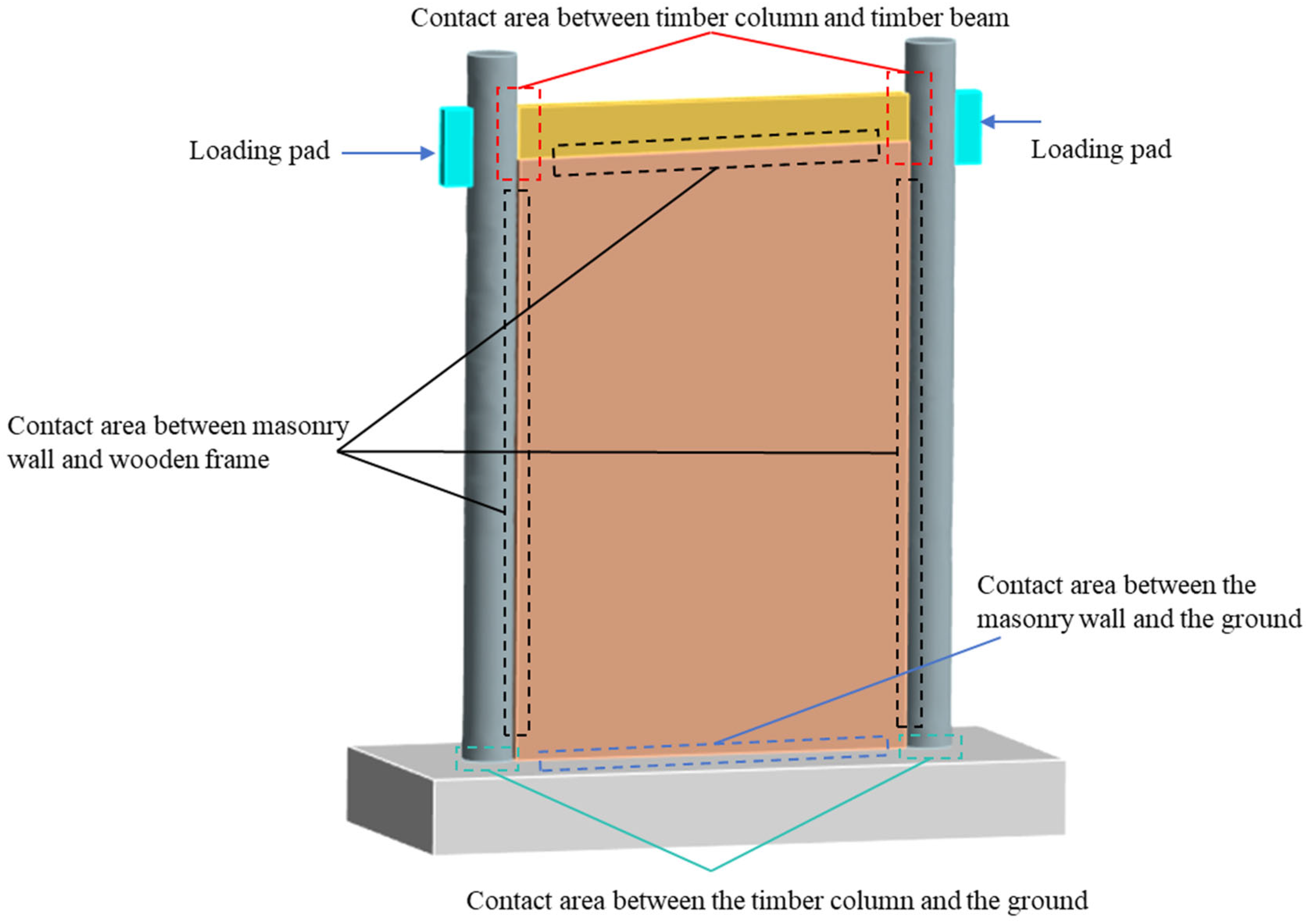
In order to further demonstrate the feasibility of conducting structural finite element analysis on the script generated by the proposed method, assumptions and completion of missing parameters in the script were made based on existing literature research. The material properties of wood and brick masonry are shown in Table 5. The contact relationship between different components is shown in Table 6, and the location of these contact areas is shown in Figure 9. Simulate a set of horizontal overturning loads using displacement loading mode (as shown in Figure 10). Import the APDL script with completed parameters into the ANSYS working platform, and the deformation diagram of the model is shown in Figure 10.
Table 5.
Assumed material parameters.
Table 6.
Assumed contact relationship.

Figure 9.
Contact area diagram.
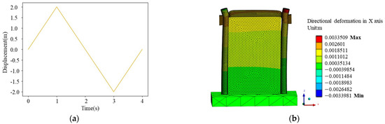
Figure 10.
Finite element analysis case: (a) loading protocol; (b) deformation cloud map.
The results indicate that the geometric finite element model proposed in this article can be used for structural analysis after completing the corresponding parameters.
4. Conclusions
This study proposed an effective method for automatically generating geometric finite element (FE) models of timber structures directly from 3D LiDAR point clouds. The key contribution to the state of the art lies in developing a fully automated end-to-end pipeline that integrates boundary inference and contact relationship analysis to robustly overcome data incompleteness caused by occlusions. This novel integration enables accurate reconstruction of hidden geometries where prior methods require manual intervention.
Validated on a representative timber structure, the method demonstrated high accuracy, with dimensional relative errors consistently below 3% when comparing the automatically generated geometric model to the actual structure. Furthermore, the geometric model generation from point cloud to executable APDL script was achieved in approximately 9.75 s, showcasing significant gains in efficiency compared to manual or semi-automated state-of-practice approaches. Perpendicularity verification of planar elements further confirmed the accuracy and robustness of the proposed algorithm.
By automating segmentation, geometric feature extraction, and parametric APDL script generation, this framework significantly reduces the time and expertise required for FE modeling of timber structures. Future work will investigate deep learning techniques to enhance segmentation performance for geometrically complex timber components.
Author Contributions
Conceptualization, L.C. and H.X.; methodology, L.C.; investigation, L.J.; writing—original draft preparation, L.C.; visualization, L.J.; funding acquisition, L.C. All authors have read and agreed to the published version of the manuscript.
Funding
This research was funded by the National Natural Science Foundation of China (52308327).
Data Availability Statement
The raw data supporting the conclusions of this article will be made available by the authors on request.
Conflicts of Interest
The authors declare that they have no competing interests.
References
- Chen, J.; Xiong, H.; Wang, Z.; Liu, Y. Experimental buckling performance of eucalyptus-based oriented oblique laminated strand lumber columns under centric and eccentric compression. Constr. Build. Mater. 2020, 262, 120072. [Google Scholar] [CrossRef]
- Cao, J.; Xiong, H.; Chen, L. Procedure for parameter identification and mechanical properties assessment of CLT connections. Eng. Struct. 2019, 203, 109867. [Google Scholar] [CrossRef]
- Yuan, C.; Zhang, J.; Chen, L.; Xu, J.; Kong, Q. Timber moisture detection using wavelet packet decomposition and convolutional neural network. Smart Mater. Struct. 2021, 30, 035022. [Google Scholar] [CrossRef]
- Di Re, P.; Lofrano, E.; Ciambella, J.; Romeo, F. Structural analysis and health monitoring of twentieth-century cultural heritage: The Flaminio Stadium in Rome. Smart Struct. Syst. 2021, 2, 27. [Google Scholar]
- Andrea, U.; Alessandro, G.; Francesca, M.; Marco, Z. From scan-to-BIM to a structural finite elements model of built heritage for dynamic simulation. Autom. Constr. 2022, 142, 104518. [Google Scholar]
- Ventura, C.; Brincker, R.; Dascotte, E.; Andersen, P. FEM updating of the heritage court building structure. In Proceedings of the IMAC 19: A Conference on Structural Dynamics, Kissimmee, FL, USA, 5–8 February 2001. [Google Scholar]
- Lord, J.-F.; Ventura, C.E.; Dascotte, E. Automated model updating using ambient vibration data from a 48-storey building in Vancouver. In Proceedings of the 22nd International Modal Analysis Conference, Detroit, MI, USA, 26–29 January 2004. [Google Scholar]
- Lord, J.-F.; Ventura, C.E.; Dascotte, E.; Brincker, R. FEM updating using ambient vibration data from a 48-storey building in Vancouver, British Columbia, Canada. In Inter Noise & Noise Con Congress & Conference Proceedings, Proceedings of the 32nd International Congress and Exposition on Noise Control Engineering, Seogwipo, Republic of Korea, 25–28 August 2003; Institute of Noise Control Engineering: Washington, DC, USA, 2003. [Google Scholar]
- Steiner, B.; Mousavian, E.; Saradj, F.M.; Wimmer, M.; Musialski, P. Integrated structural–architectural design for interactive planning. In Computer Graphics Forum; Wiley Online Library: Hoboken, NJ, USA, 2017; Volume 36, pp. 80–94. [Google Scholar]
- Boonstra, S.; Blom, K.V.; Hofmeyer, H.; Emmerich, M.T. Hybridization of an evolutionary algorithm and simulations of co-evolutionary design processes for early-stage building spatial design optimization. Autom. Constr. 2021, 124, 103522. [Google Scholar] [CrossRef]
- Boonstra, S.; Blom, K.V.; Hofmeyer, H.; Emmerich, M.T.; Schijndel, J.; Wilde, P. Toolbox for super-structured and super-structure free multi-disciplinary building spatial design optimisation. Adv. Eng. Inform. 2018, 36, 86–100. [Google Scholar] [CrossRef]
- Bouzas, Ó.; Cabaleiro, M.; Conde, B.; Cruz, Y.; Riveiro, B. Structural health control of historical steel structures using HBIM. Autom. Constr. 2022, 140, 104308. [Google Scholar] [CrossRef]
- Mol, A.; Cabaleiro, M.; Sousa, H.S.; Branco, J. HBIM for storing life-cycle data regarding decay and damage in existing timber structures. Autom. Constr. 2020, 117, 103262. [Google Scholar] [CrossRef]
- Yang, L.; Cheng, J.C.; Wang, Q. Semi-automated generation of parametric BIM for steel structures based on terrestrial laser scanning data. Autom. Constr. 2020, 112, 103037. [Google Scholar] [CrossRef]
- Romero-Jarén, R.; Arranz, J.J. Automatic segmentation and classification of BIM elements from point clouds. Autom. Constr. 2021, 124, 103576. [Google Scholar] [CrossRef]
- Zhang, C.; Shu, J.; Shao, Y.; Zhao, W. Automated generation of FE models of cracked RC beams based on 3D point clouds and 2D images. J. Civ. Struct. Health Monit. 2022, 12, 29–46. [Google Scholar] [CrossRef]
- Che, E.; Jung, J.; Olsen, M.J. Object recognition, segmentation, and classification of mobile laser scanning point clouds: A state of the art review. Sensors 2019, 19, 810. [Google Scholar] [CrossRef] [PubMed]
- Lu, R.; Brilakis, I. Detection of structural components in point clouds of existing RC bridges. Comput.-Aided Civ. Infrastruct. Eng. 2019, 34, 191–212. [Google Scholar] [CrossRef]
- Hamid-Lakzaeian, F. Point cloud segmentation and classification of structural elements in multi-planar masonry building facades. Autom. Constr. 2020, 118, 103232. [Google Scholar] [CrossRef]
- Qi, C.R.; Su, H.; Mo, K.; Leonidas, J. Pointnet: Deep learning on point sets for 3d classification and segmentation. In Proceedings of the IEEE Conference on Computer Vision and Pattern Recognition, Honolulu, HI, USA, 21–26 July 2017. [Google Scholar]
- Qi, C.R.; Yi, L.; Su, H.; Leonidas, J. Pointnet++: Deep hierarchical feature learning on point sets in a metric space. In Proceedings of the Advances in Neural Information Processing Systems, Long Beach, CA, USA, 4–9 December 2017. [Google Scholar]
- Li, Y.; Bu, R.; Sun, M.; Wu, W.; Di, X.; Chen, B. Pointcnn: Convolution on x-transformed points. In Proceedings of the Advances in Neural Information Processing Systems, Montréal, QC, Canada, 3–8 December 2018. [Google Scholar]
- Lee, J.S.; Park, J.; Ryu, Y.M. Semantic segmentation of bridge components based on hierarchical point cloud model. Autom. Constr. 2021, 130, 103847. [Google Scholar] [CrossRef]
- Kim, H.; Yoon, J.; Sim, S.H. Automated bridge component recognition from point clouds using deep learning. Struct. Control Health Monit. 2020, 27, e2591. [Google Scholar] [CrossRef]
- Arayici, Y. Towards building information modelling for existing structures. Struct. Surv. 2008, 26, 210–222. [Google Scholar] [CrossRef]
- Pătrăucean, V.; Armeni, I.; Nahangi, M.; Yeung, J.; Brilakis, I.; Haas, C. State of research in automatic as-built modelling. Adv. Eng. Inform. 2015, 29, 162–171. [Google Scholar] [CrossRef]
- Arias, P.; Armesto, J.; Lorenzo, H.; Ordóñez, C. Digital photogrammetry, GPR and finite elements in heritage documentation: Geometry and structural damages. In Proceedings of the ISPRS Commission V Symposium: Image Engineering and Vision Metrology, Dresden, Germany, 25–27 September 2006. [Google Scholar]
- Lu, R.; Brilakis, I. Digital twinning of existing reinforced concrete bridges from labelled point clusters. Autom. Constr. 2019, 105, 102837. [Google Scholar] [CrossRef]
- Kassotakis, N.; Sarhosis, V.; Mills, J.; Antonio, M. From point clouds to geometry generation for the detailed micro-modelling of masonry structures. In Proceedings of the 10th International Masonry Conference, Milan, Italy, 9–11 July 2018. [Google Scholar]
- Barazzetti, L.; Banfi, F.; Brumana, R.; Gusmeroli, G.; Previtali, M.; Schiantarelli, G. Cloud-to-BIM-to-FEM: Structural simulation with accurate historic BIM from laser scans. Simul. Model. Pract. Theory 2015, 57, 71–87. [Google Scholar] [CrossRef]
- Jiang, S.; Yang, Y.; Gu, S.; Li, J.; Hou, Y. Bridge Geometric Shape Measurement Using LiDAR–Camera Fusion Mapping and Learning-Based Segmentation Method. Buildings 2025, 15, 1458. [Google Scholar] [CrossRef]
- Wang, D.; Liu, J.; Jiang, H.; Liu, P.; Jiang, Q. Existing Buildings Recognition and BIM Generation Based on Multi-Plane Segmentation and Deep Learning. Buildings 2025, 15, 691. [Google Scholar] [CrossRef]
- Patil, J.; Mohsen, K. Automatic Scan-to-BIM—The Impact of Semantic Segmentation Accuracy. Buildings 2025, 15, 1126. [Google Scholar] [CrossRef]
- Proença, P.F.; Gao, Y. Fast cylinder and plane extraction from depth cameras for visual odometry. In Proceedings of the 2018 IEEE/RSJ International Conference on Intelligent Robots and Systems (IROS), Madrid, Spain, 1–5 October 2018. [Google Scholar]
- Mathew, V.; Amin, R. Optimizing Fast-Paced Sacn-to-BIM Projects Using ReCap, Revit, Navisworks. Available online: https://www.autodesk.com/autodesk-university/class/Optimizing-Fast-Paced-Scan-BIM-Projects-Using-ReCap-Revit-Navisworks-2018 (accessed on 4 February 2019).

Disclaimer/Publisher’s Note: The statements, opinions and data contained in all publications are solely those of the individual author(s) and contributor(s) and not of MDPI and/or the editor(s). MDPI and/or the editor(s) disclaim responsibility for any injury to people or property resulting from any ideas, methods, instructions or products referred to in the content. |
© 2025 by the authors. Licensee MDPI, Basel, Switzerland. This article is an open access article distributed under the terms and conditions of the Creative Commons Attribution (CC BY) license (https://creativecommons.org/licenses/by/4.0/).