DYMOS: A New Software for the Dynamic Identification of Structures

Abstract

Operational modal analysis (OMA) is widely used for its simplicity and reliance on ambient noise. While commercial OMA software exists, they often limit user control. Some researchers develop their own tools, but independent software tools remain scarce. The number of such independent software is limited, and the development of new ones with enhanced features, better performance, and varied user interfaces would be beneficial to spread the informed use of dynamic identification techniques, leading to more reliable and valuable results for structural engineering applications. This work introduces the new DYMOS software for OMA from ambient vibration test recordings. DYMOS includes various state-of-art algorithms and tools for vibration-based modal identification and for optimal sensor placement (OSP), allowing for customization of analysis parameters and procedures with the aim of reducing the gap between the needs of professional practice and research. Additionally, a new graphical tool is introduced for visualizing results in both buildings and bridges. By using CAD drawings as input, it streamlines model construction, making the process faster, more intuitive, and efficient. The article aims to describe DYMOS and to demonstrate its potential for OMA and OSP in civil engineering through the application on two real case studies dynamically tested.

1. Introduction

Operational modal analysis (OMA) has emerged as a vital tool in the realm of civil engineering, offering valuable insights into the dynamic behavior of structures under real operating conditions [1]. Unlike traditional modal analysis techniques that rely on controlled excitation, OMA extracts modal parameters from ambient vibrations induced by natural environmental forces or operational activities (the so-called ambient noise). The modal parameters include natural frequencies, mode shapes, and damping ratios, which play a crucial role in understanding structural performance, safety, and serviceability of structures [2].

In civil engineering, the uses of OMA results are multifaceted. Firstly, OMA facilitates the identification and characterization of dynamic properties of civil engineering structures [3,4,5]. By analyzing the modal parameters extracted through OMA, engineers gain a deeper understanding of the structural response to various dynamic loading conditions, including wind, traffic, and seismic events [6]. Several works in the literature report the successful application of OMA across a wide range of modern structural typologies, e.g., buildings [7], bridges [8], dams [9], stadiums [10], and also ancient structures, e.g., masonry arch bridges [11], churches [12], towers [13], and palaces [14]. Furthermore, OMA is applied in performing the so-called dynamic proof tests of structures; during stage construction and at the end, through which engineers can validate the design assumptions, evaluate the adequacy of structural components; and in identifying potential weaknesses or vulnerabilities that may compromise the safety or serviceability of the structure [15,16]. Also, OMA findings are fundamental in the structural health monitoring (SHM) framework, allowing engineers to continuously assess the condition of structures throughout their service life. By monitoring changes in modal parameters over time, such as shifts in natural frequencies, alterations in mode shapes, or the occurrence of abnormal values of damping ratios, OMA aids in the early detection of structural damage, deterioration, and performance degradation [17,18]. This proactive approach to maintenance and monitoring helps mitigating risks, enhance safety, and optimize maintenance strategies, ultimately prolonging the lifespan of civil engineering structures and infrastructures.

Nowadays, several software packages for OMA are commercially available, and they vary in terms of features, capabilities, and compatibility with different measurement systems and hardware. The most popular ones are MATLAB OMA Toolbox, developed by the Structural Dynamics Research Group at KU Leuven; ARTeMIS, developed by Structural Vibration Solutions; ME’scopeVES, developed by Vibrant Technology; Modal Analysis & Controls Toolkit (MACT), which is a toolkit for LabVIEW developed by National Instruments; Pulse Reflex, developed by B&K; and S2-OMA, developed by S2X. However, the algorithms of these software are often closed to the user, who can only vary some input data. For this reason, some researchers have independently developed software for OMA in order to be able to investigate this topic more thoroughly and test new identification strategies. Many works are available in the literature proposing automatic modal identification tools to be used within continuous dynamic monitoring frameworks, while only a few deal with identification tools designed to analyze one-time dynamic tests. For instance, García-Macías and Ubertini propose a software called MOVA for the dynamic identification of structures [19], which is then coupled with a software for SHM (the latter called MOSS). Also, Pasca et al. [20] propose a software (called PyOMA) developed in Python environment for estimating the operational modal parameters of a structure from output-only vibration measurements in operational conditions. However, the number of such independent software tools is limited, and the development of new ones with enhanced features, better performance, and varied user interfaces would be beneficial to spread the informed use of dynamic identification techniques, leading to more reliable and valuable results for structural engineering applications.

In this work, the new DYMOS (DYnamic MOnitoring of Structures) software for the dynamic identification of structures from AVT recordings is presented. DYMOS gathers in separate modules a collection of the state-of-art algorithms and tools for vibration-based (VB) modal identification and optimal sensor placement (OSP) of structures with the possibility of customizing multiple analysis parameters with the aim of reducing the gap between the needs of professional practice and research. Indeed, this software is conceived for allowing the expert user to operate different choices about methods and parameters to be used until obtaining with awareness a satisfactory result while helping the less experienced user to easily achieve results as well. Furthermore, a new graphical tool is implemented for visualizing results in both buildings and bridges. It simplifies model construction by using CAD drawings as input, making the process faster, more intuitive, and efficient. The scope of this article is to describe the DYMOS software and to show its potentiality for the OMA and OSP of civil engineering structures. To these aims, two real case studies (dynamically tested with AVTs in the recent past) are identified and studied by using the proposed software. All software modules and procedures are in-depth illustrated with reference to the case studies. Additionally, general suggestions are given to the reader on the procedures and parameters to be used for the dynamic identification of such structures. Concerning the paper contents, Section 2 describes the software architecture and its main strengths, as well as its innovative features compared with the existing tools. Section 3 is devoted to introduce the case studies, while in Section 4, the pre-processing of accelerometric signals is addressed. In Section 5, the system identification process is deeply addressed, also treating the basis of the adopted identification methodologies. This section also contains an exhaustive discussion about the mode selection procedure (manual or automatic), which is a strength of this software. Then, in Section 6, the module for the result merging in case of multi-set-up tests is discussed. In Section 7, the innovative tool for the mode shape plot is presented. Finally, Section 8 is devoted to describing the OSP part and the relevant applications to the two case studies.

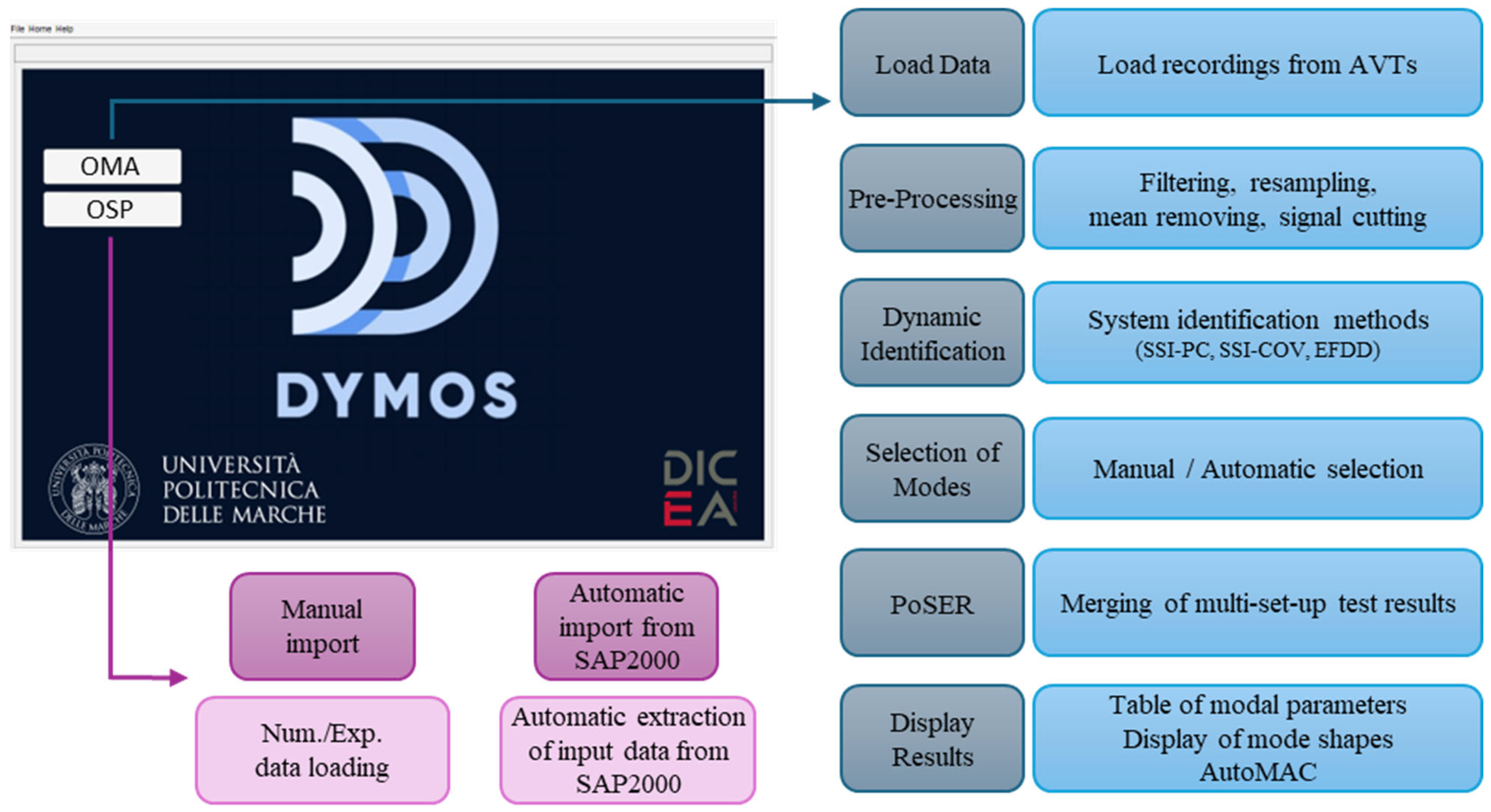
2. Description of the Software Architecture

DYMOS is a software developed in MATLAB environment that is suitable for the comprehensive dynamic identification of structures. To the best of the authors’ knowledge, it is the first software containing the following two main parts (Figure 1): one to perform the OMA, while another to perform the OSP. These two tasks are closely interconnected, as the OSP is a fundamental component for conducting accurate AVTs and the corresponding OMA. In the first part (OMA), a user may find modules for pre-processing of the original data, modal identification, mode selection, merging data from several AVT configurations, and graphical representation of results. The second part (OSP) consists of two modules that differ in how input data is provided. The first module requires manual input, making it compatible with both numerical models and experimental results. The second module automatically loads data from a commercial software (SAP2000), limiting its use to numerical applications.

Thanks to the intuitive graphical user interface, the DYMOS software is suitable for both experienced users and beginners approaching the subject of dynamic identification of structures for the first time. DYMOS stands out from other software due to several key strengths. For example, its mode selection module is separated from the identification module, ensuring a clearer and more customizable mode selection process. Moreover, this choice allows the mode selection to be performed many times without having to repeat the system identification too, considerably reducing the computational efforts. In addition to the classical manual selection of modes, it is also possible to perform a guided mode selection based on criteria adopted in automatic identification algorithms. This dual choice enables expert users to quickly and repeatedly adjust the selection of solutions, allowing them to consciously arrive at a satisfactory and appropriate outcome while assisting less experienced users in determining which modes can be considered real modes of the tested structure. Then, input parameters for mode identification and clustering are fully customizable, thus making the software also suitable for research purposes. In addition, a new tool for the graphical representation of results is implemented, which is suitable for both buildings and bridges. This innovative tool has the great advantage of using CAD drawings (i.e., files in .dxf format) as geometry input data instead of a list of geometric coordinates, making the construction of the geometric model and of the experimental measurement grid much simpler, faster, and more intuitive. Finally, differently from the existing software for the dynamic identification of structures, DYMOS also includes a sub-section for the development of OSP analyses starting from either numerical model outcomes or experimental identification results. The latter is of paramount importance during the planning of dynamic tests, as well as when SHM systems are designed.

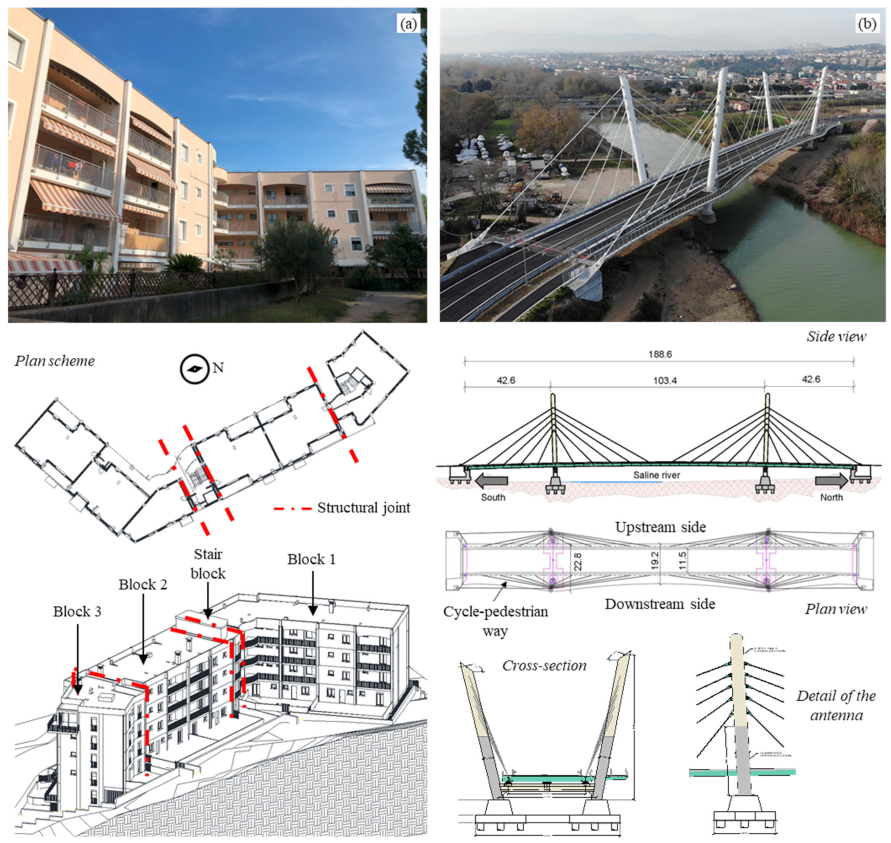
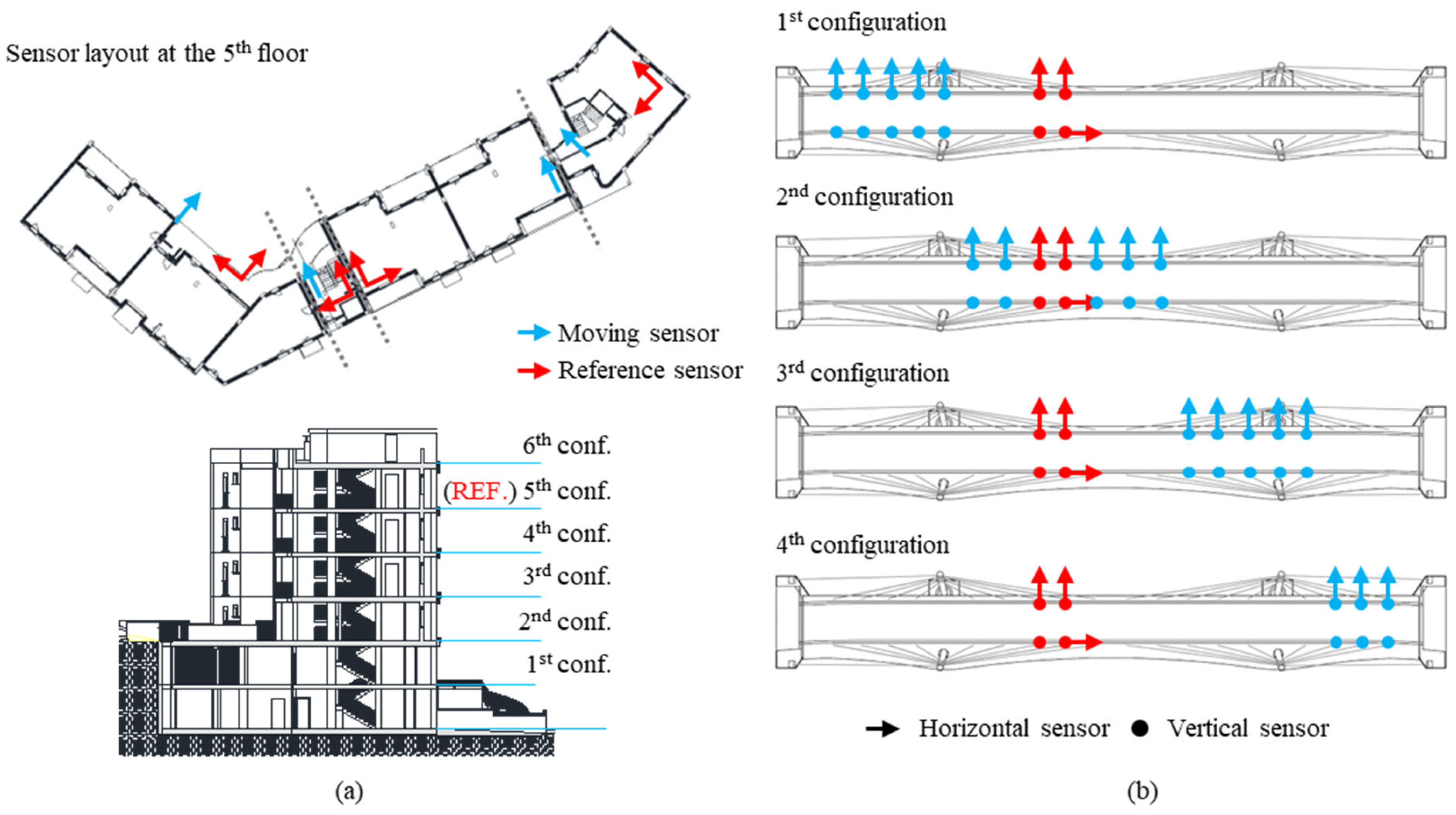
3. Introduction to the Case Studies

In this work, the software potentiality is shown for the dynamic identification of two civil engineering structures that were tested through AVTs. These are articulated structures with complex geometries characterized by non-trivial dynamic behavior requiring a careful and non-simple modal identification phase. The former is a multi-block residential building located in Central Italy (Figure 2a). The whole building is composed of four blocks with RC frame structure and masonry infills separated by structural joints. Planimetrically, the edifice has an almost “L” shape, with a greater length of about 44 m and a lower one of 28 m. All blocks are approximatively 11 m wide and composed of six elevations, for a total height of 18.5 m. The second case study is a newly built cable-stayed bridge located in Central Italy (Figure 2b). The bridge, about 190 m long, has a continuous steel–concrete composite deck with two traffic lanes, with variable width ranging from 19.2 to 22.8 m, and it is supported by 40 diagonal stays. The downstream side of the deck was designated with a curved layout to host a cycle and pedestrian way. Both structures were dynamically tested through AVTs to capture their whole dynamic behavior. The adopted sensors were uniaxial piezoelectric accelerometers with 10,000 mV/g of nominal sensibility and a ±0.5 g measurement range, connected by coaxial cables to three-channel acquisition modules NI-9230 mounted on both four-slot NI cDAQ-9185 and eight-slot NI cRIO-9045 chassis. The acquisition modules were linked together by means of ethernet cables. A self-made software with LabVIEW was used to acquire and save the data.

4. Signal Pre-Processing

4.1. Module for Loading Signal Recordings

The first module of the software (“Load Data”) allows for the loading of signals recorded during dynamic tests with the aim of checking their goodness and detecting any anomalies, also performed by visualizing the relevant spectrum (Figure 3). After selecting the file to be uploaded, the software automatically recognizes the number of columns within the file, which corresponds to the number of the recorded measurement channels (equal to the total number of measurement direction of all the sensors). The user may assign a customized name to each channel, which usually corresponds to the same name assigned at the dynamic test design stage. Then, the correctness of the channel name can be checked by means of the “View Geometry” button, which displays the complete geometry of the tested structure with indication of the direction and the name of each measurement channel. Details on how to create this geometry will be provided later in a dedicated section (Section 7). Another key parameter to be entered at this stage is the signal sampling frequency. By clicking on the “Compute PSD” button, the software allows the power spectral density (PSD) of each signal to be calculated and displayed up to the Nyquist frequency. By acting on the check boxes in the right-hand side menu, it is possible to select the channel to be displayed in the graphs, also being active the option of displaying several channels simultaneously and superimposed. An example of the use of this module and the display of signals and spectrum can be found in Figure 3 for recordings of a dynamic test performed on the building case study.

4.2. Signal Pre-Processing Module

Signal pre-processing is a fundamental step before using measured data as it helps eliminate most noise effects and any abnormal events, ensuring that the processed signals comply with the white noise assumption. The “Pre-Processing” module of the software (Figure 4) allows the common pre-processing procedures to be performed both together and separately by activating the check box of the relevant procedure. The original signal can be filtered by using a Butterworth filter and selecting one of the three most common filter types (low, bandpass, and high). For both case studies, a bandpass filter is used, but with different cutting frequencies (F_cut): the interval 0.1–10 Hz is chosen for the building, while 0.1–2 Hz is chosen for the bridge, being the latter a more flexible structure. The down-sampling frequency could be set to reduce the amount of data and perform faster subsequent analyses. In both case studies, the adopted frequency sampling during the dynamic tests was 1024 Hz due to characteristics of the adopted instrumentation; consequently, a reduced amount of data is employed to perform the modal identification, choosing a re-sampling frequency of 102.4 Hz. Furthermore, linear detrending could be performed as well. Before running the aforementioned pre-processing techniques, parameters to compute the Welch’s PSD estimate have to be provided by the user; the authors suggest using 20 s for the signal windowing with 10 s of overlapping.

The post-processed time histories are then plotted flanked by the PSDs of the original (blue line) and post-processed (orange line) signals in order to individuate possible signal corruption due to the pre-processing procedure. By analyzing these plots, it is also possible to find those parts of the signal that can be manually cut by the user (by defining time intervals in the dedicated table on the top right corner) because of the presence of abnormal events that are not removed by the pre-processing procedure. An example is shown for a dynamic test of the building case study, where the first 10 s and 2 s around a signal spike are removed. The cut signal and the relevant spectrum are plotted below the original (complete) one to control the correctness of the pre-processing activities.

At the end of the procedure, the software allows for the saving of the pre-processed data in a dedicated .csv format file. This makes it possible to obtain pre-processed data packages that can be used whenever deemed necessary, without having to repeat the procedure when a new work session is started on the same data.

5. System Identification

5.1. Basics on the Identification Methods

The software allows for the use of three different identification methods, two of them working in the time and one in the frequency domain. A brief resume of the basic theory of these methods is provided below for clarity and for the better understating of a non-expert reader. Regarding time domain methods, the stochastic subspace identification (SSI) is one of the most widely adopted. SSI means that the structure is excited by unmeasurable input forces and only output measurements (e.g., accelerations) are available. In these identification methods, the deterministic knowledge of the input is replaced by the assumption that the input is a realization of a stochastic process (white noise) [21].

A brief recall of SSI basis is herein reported. Starting from the discrete time formulation, the equation of motion of a multi-degrees-of-freedom (multi-DOF) system can be written as:

$$\mathbf{M}\ddot{\mathit{u}}\left(t\right)+\mathbf{E}\dot{\mathit{u}}\left(\mathit{t}\right)+\mathbf{K}\mathit{u}\left(t\right)=\mathbf{f}\left(t\right)$$

(1)

where M, E, and K are the mass, damping, and stiffness matrices with dimension n × n, where n represents the system DOFs, and f(t) is the loading vector. Equation (1) can be written in matrix form as:

$$\left(\begin{array}{cc}\mathit{E}& \mathit{M}\\ \mathit{M}& 0\end{array}\right)\left(\begin{array}{c}\dot{\mathit{u}}\left(t\right)\\ \ddot{\mathit{u}}\left(t\right)\end{array}\right)+\left(\begin{array}{cc}\mathit{K}& 0\\ 0& -\mathit{M}\end{array}\right)\left(\begin{array}{c}\mathit{u}\left(t\right)\\ \dot{\mathit{u}}\left(t\right)\end{array}\right)=\left(\begin{array}{c}\mathit{I}\\ 0\end{array}\right)\mathbf{f}(t)$$

(2)

If we define the state vector x(t) and matrices P and Q as:

$$\mathit{x}\left(t\right)=\left(\begin{array}{c}\mathit{u}\left(t\right)\\ \dot{\mathit{u}}\left(t\right)\end{array}\right); \mathbf{P}=\left(\begin{array}{cc}\mathit{E}& \mathit{M}\\ \mathit{M}& 0\end{array}\right); \mathbf{Q}=\left(\begin{array}{cc}\mathit{K}& 0\\ 0& -\mathit{M}\end{array}\right)$$

(3)

the second-order equation of motion (Equation (2)) simplifies to a first-order equation:

$$\mathbf{P}\dot{\mathit{x}}(t)+\mathbf{Q}\mathit{x}(t)=\left(\begin{array}{c}\mathit{I}\\ 0\end{array}\right)\mathbf{f}(t)$$

(4)

Multiplying Equation (4) by P⁻¹, we obtain:

$$\dot{\mathit{x}}\left(t\right)=\mathbf{A}\mathit{x}\left(t\right)+\mathbf{B}\mathbf{f}\left(t\right)$$

(5)

with

$$\mathbf{A}=\left(\begin{array}{cc}0& \mathit{I}\\ -{\mathit{M}}^{-1}\mathit{K}& -{\mathit{M}}^{-1}\mathit{E}\end{array}\right); \mathbf{B}=\left(\begin{array}{c}0\\ {\mathit{I}\mathit{M}}^{-1}\end{array}\right)$$

(6)

being A the so-called state space matrix with dimension 2n × 2n. Considering that in an output-only dynamic test the recordings are performed in only some DOFs, the observation equation can be defined as:

$$\mathit{y}\left(t\right)={\mathit{C}}_{\mathit{a}}\ddot{\mathit{u}}\left(t\right)+{\mathit{C}}_{\mathit{v}}\dot{\mathit{u}}\left(\mathit{t}\right)+{\mathit{C}}_{\mathit{d}}\mathit{u}\left(t\right)$$

(7)

where C_a, C_v, and C_d are Boolean matrices that select the l measured DOFs. Isolating $\ddot{\mathit{u}}\left(t\right)$ from Equation (1) and substituting it into Equation (7), the observability equation can be determined as:

$$\mathit{y}\left(t\right)=\mathbf{C}\mathit{x}\left(t\right)+\mathbf{D}\mathbf{f}\left(t\right)$$

(8)

with

$$\mathbf{C}=\left(\begin{array}{cc}{\mathit{C}}_{\mathit{d}}-{\mathit{C}}_{\mathit{a}}{\mathit{M}}^{-1}\mathit{K}& {\mathit{C}}_{\mathit{v}}-{\mathit{C}}_{\mathit{a}}{\mathit{M}}^{-1}\mathit{E}\end{array}\right); \mathbf{D}={\mathit{C}}_{\mathit{a}}{\mathbf{M}}^{-1}$$

(9)

Equations (5) and (8) constitute together the equation of motion formulated into the state space. These equations need to be transformed into the discrete time because the real measurements are taken at discrete time instants; by defining a discrete time interval ∆T, the time t can be defined as $t=k∆T$. Furthermore, in output-only dynamic tests, the input is not measured but assumed as white noise; so, the state space model becomes:

$$\begin{gathered} {\mathit{x}}_{k+1}=\mathbf{A}{\mathit{x}}_{\mathit{k}}+{\mathit{w}}_k \\ {\mathit{y}}_k=\mathbf{C}{\mathit{x}}_{\mathit{k}}+{\mathit{v}}_k \end{gathered}$$

(10)

where w_k and v_k are unmeasurable vectors assumed as zero-mean signal (white noise). Equation (10) can be used to determine the system response at each k instant (${\mathit{y}}_k$) if the system properties are known (A and C), as well as its initial state (${\mathit{x}}_0$). To determine A and C matrices, identification algorithms working in the state space (SSI-COV and SSI-DATA in the software) are used.

The covariance-driven SSI (SSI-COV) [19] method identifies a stochastic state space model from the output covariance matrix. It starts by computing the output correlation matrices R₁ and R_2jb for positive time lags varying from $∆T$ to (2j_b−1)$∆T$, respectively. Afterwards, the covariance matrix is organized in a lj_b-by-lj_b block Toeplitz matrix T:

$$\mathbf{T}=\left[\begin{array}{ccc}{\mathit{R}}_{\mathit{j}\mathit{b}}& {\mathit{R}}_{\mathit{j}\mathit{b}}-1& \begin{array}{cc}\dots & {\mathit{R}}_1\end{array}\\ \begin{array}{c}{\mathit{R}}_{\mathit{j}\mathit{b}+1}\\ \dots \end{array}& \begin{array}{c}{\mathit{R}}_{\mathit{j}\mathit{b}}\\ \dots \end{array}& \begin{array}{cc}\dots & {\mathit{R}}_2\\ \dots & \dots \end{array}\\ {\mathit{R}}_{2\mathit{j}\mathit{b}-1}& {\mathit{R}}_{2\mathit{j}\mathit{b}-2}& \begin{array}{cc}\dots & {\mathit{R}}_{\mathit{j}\mathit{b}}\end{array}\end{array}\right]$$

(11)

Then, the singular value decomposition (SVD) of the block Toeplitz matrix is calculated. The number of non-zero SVs gives the rank of the decomposed matrix, which, in this case, coincides with the dimension of the state space matrix A. On the basis of the SVD, the identification of the state space model matrices A and C is straightforward.

The data-driven SSI (SSI-DATA) [22] principal component (PC) is similar to SSI-COV, but it uses the recorded time histories collected in a block Hankel matrix instead of covariance matrices. The block Hankel matrix is defined as:

$${\mathit{Y}}_{\mathit{h}}=\left[\begin{array}{c}\begin{array}{c}{\mathit{Y}}_{(1:\mathit{N}-2\mathit{s})}\\ {\mathit{Y}}_{(2:\mathit{N}-2\mathit{s}+1)}\end{array}\\ \begin{array}{c}⋮\\ {\mathit{Y}}_{(\mathit{s}:\mathit{N})}\end{array}\end{array}\right]=\left[\begin{array}{c}{\mathit{Y}}_{\mathit{h}\mathit{p}}\\ {\mathit{Y}}_{\mathit{h}\mathit{f}}\end{array}\right]$$

(12)

where Y is the measured response of the system, N is the length of recorded time histories, and 2s the total data shift. The upper half of the matrix (${\mathit{Y}}_{\mathit{h}\mathit{p}}$) is called “past” and the lower half (${\mathit{Y}}_{\mathit{h}\mathit{f}}$) is called “future”. The number of rows of the block Hankel matrix is 2sM (sM is the maximum number of eigenvalues), and the number of columns is N − 2s. In the work of Van Overschee and De Moor [23], projection is introduced as a geometric tool for the determination of matrices A and C.

To gather modal parameters from the equations of the state space model (Equation (10)), the first step is to perform an eigenvalue decomposition of the system matrix A:

$$\mathit{A}=\mathit{\Psi }\left[{\mathit{\mu }}_{\mathit{i}}\right]{\mathit{\Psi }}^{-1}$$

(13)

where ${\mathit{\mu }}_{\mathit{i}}$ and $\mathit{\Psi }$ are the eigenvalue and eigenvector of the i-th mode, respectively. The continuous time eigenvalues can be calculated from the discrete time ones by using the following relationship:

$${\mathit{\lambda }}_{\mathit{i}}={\displaystyle \frac{\mathit{l}\mathit{n}\left({\mathit{\mu }}_{\mathit{i}}\right)}{\mathit{d}\mathit{t}}}$$

(14)

where dt is the discrete time sampling of signal. Once ${\lambda }_i$ is known, modal parameters (frequency f_i, damping ratio $\xi$_i, and mode shape vector ${\mathit{\varphi }}_{\mathit{i}}$) are determined:

$$f_i={\displaystyle \frac{\left|{\mathit{\lambda }}_{\mathit{i}}\right|}{2\mathit{\pi }}}; {\xi }_i={\displaystyle \frac{\mathit{R}\mathit{e}\left({\mathit{\lambda }}_{\mathit{i}}\right)}{\left|{\mathit{\lambda }}_{\mathit{i}}\right|}}; {\mathit{\varphi }}_{\mathit{i}}=\mathbf{C}\mathbf{\Psi }$$

(15)

Parametric identification methods (such as the SSI approach used in this study) face a significant challenge: the need to predefine the dynamic system order (i.e., the number of degrees of freedom). A common strategy to address this issue involves performing the identification across a range of model orders, selected within a predefined interval. This process yields multiple estimates of the modal parameters for each vibration mode, which are then visualized using a stabilization diagram. This inevitably leads to the occurrence of non-physical modes, called spurious poles, which have to be isolated from the real ones and discarded from results. In practice, the order of the model is updated by varying the number of singular values taken into account when performing the singular decomposition of the projection matrix in SSI-DATA. Instead, in SSI-COV, the diagram is built by increasing the number of singular values and vectors of the Toeplitz matrix. The stable poles represent the physical solutions of the system.

Considering the frequency domain, the enhanced frequency domain decomposition (EFDD) [24] method is implemented within the software. The EFDD implies that modes are identified by simple peak-peaking, locating the peaks in SVD plots calculated from the spectral density spectra of the responses [25]. This method is suitable when peaks of modes are clearly identifiable in the frequency domain signal, while it becomes less usable in the case of closed-spaced modes. The EFDD technique is based on the fast Fourier transform analysis (FFT), and the accuracy of the estimated natural frequency depends on the FFT resolution. In the EFDD technique, the simple-DOF PSD function, identified around a peak of resonance, is taken back to the time domain by using the inverse discrete Fourier transform. The natural frequency is obtained by determining the number of zero-crossing as a function of time, and the damping by the logarithmic decrement [26]. In this technique, the relationship between the unknown input and the measured responses can be expressed as:

$$\left[{\mathit{G}}_{\mathit{y}\mathit{y}}\left(j\omega \right)\right]={\left[\mathit{H}\left(j\omega \right)\right]}^I\left[{\mathit{G}}_{\mathit{x}\mathit{x}}\left(j\omega \right)\right]{\left[\mathit{H}\left(j\omega \right)\right]}^T$$

(16)

where ${\mathit{G}}_{\mathit{x}\mathit{x}}\left(j\omega \right)$ is a r × r PSD matrix of the input, r is the number of inputs, ${\mathit{G}}_{\mathit{y}\mathit{y}}\left(j\omega \right)$ is a l × l PSD matrix of the responses, and $\mathbf{H}\left(j\omega \right)$ is a l × r FRF matrix. In Equation (16), symbols “^I” and “^T” denote the conjugate and transpose, respectively. In the EFDD, the first step is to estimate the PSD matrix of the response at discrete frequencies $\mathsf{\omega }={\omega }_i$; then, it is decomposed by taking the SVD:

$$\left[{\mathit{G}}_{\mathit{y}\mathit{y}}\left(j{\omega }_i\right)\right]={\mathit{U}}_i{\mathit{S}}_i{\mathit{U}}_i^H$$

(17)

where the matrix U_i holds the singular vectors u_ij, and S_i is a diagonal matrix holding the scalar singular values s_ij. The first singular vector u_ij is an estimation of the mode shape. For each ${\omega }_i$, the first SV of the PSD function is analyzed around the peak by comparing the mode shape estimation u_ij with the singular vectors around the selected peak. As long as a singular vector with high modal assurance criterion (MAC) value with u_ij is found, the corresponding first SV is assumed belonging to the simple-DOF density function of the investigated mode ${\omega }_i$. The piece of the simple-DOF PSD can be taken back to time domain by inverse FFT, and the natural frequency and damping ratios are simply estimated from the crossing times and by using the logarithmic decrement.

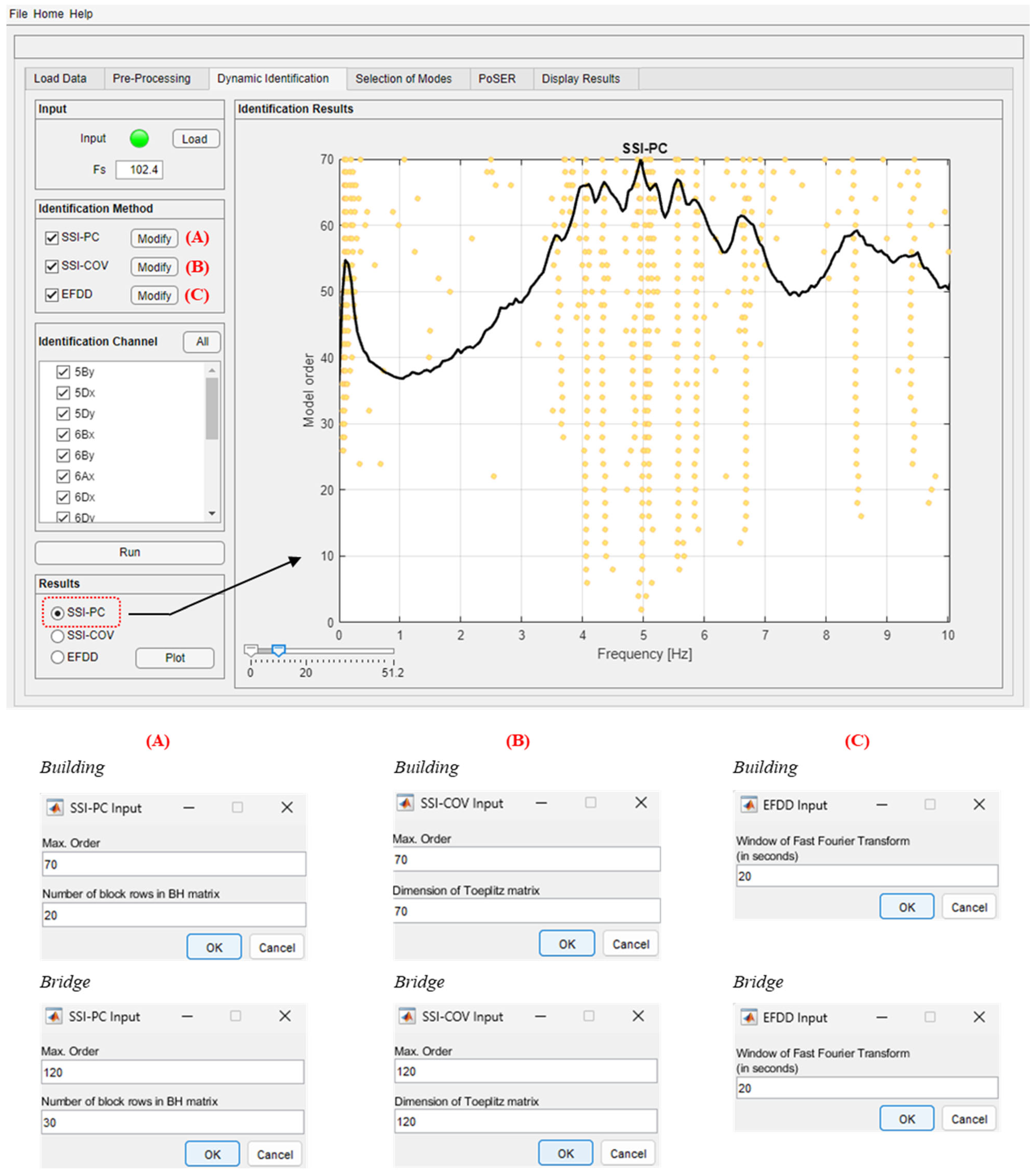
5.2. Dynamic Identification Module

The “Dynamic Identification” module allows the system dynamic identification and the display of the relevant results to be performed. The methods implemented for the modal identification in the DYMOS software are well established and robust, allowing for the identification of a structural system regardless of the sensor layout used. This module makes it possible to operate in continuity with the previous pre-processing phases or to directly load a file collecting pre-processed recordings already available. Obviously, in both cases, the sampling frequency (Fs, original or re-sampled) must be entered. The three identification methods can be selected either individually or together and, when selecting one method, the input parameters must be inserted. In Figure 5, the parameters adopted for the dynamic identification of both case studies and for all three methods are reported. These parameters are obtained after several tests and are the ones that led to the most accurate modal identification.

As an additional option, the user can also select the measurement channels that are used in the identification process in order to carry out either modal identifications with the full set of recordings or with a reduced set of channels. Once the identification is complete, the results for each selected method can be displayed. For time domain methods, the stabilization diagram is displayed with all the identified solutions (represented with yellow dots) superimposed to the 1st SV of the signal spectra (Figure 5). The stabilization diagram is built with a minim model order equal to two (as a default setting) and increasing it by two units at a time up to the maximum order defined by the user. For the EFDD method, only the first SV is displayed at this phase.

5.3. Selection of Modes

The selection of the identified modes can be performed in two alternative ways, manually or automatically. The manual selection, although guided, presupposes a thorough knowledge of the subject by the user. The automatic selection (commonly known as AutoOMA) allows the software to automatically select the stable modes of the system on the basis of a clustering method by simply defining few input parameters. However, even in this case, a basic knowledge of the subject by the user is required in order to avoid defining unrealistic input parameters and, thus, obtaining unreliable results.

After the mode selection, the obtained results are reported in terms of modal parameters for each selected mode. More specifically, a table collecting frequency, damping ratio and modal complexity factor (MCF) values for each mode is reported, together with the modal complexity plot that varies selecting modes in the table. Also, the AutoMAC calculated between all the selected solutions is shown in the relevant AutoMAC matrices. The results can be saved in a dedicated .xlsx format file that collects the frequency, damping ratio, MCF, and modal displacement normalized with respect to the maximum value of each mode. As an example, the modal identification results for the two case studies are reported in Figure 6.

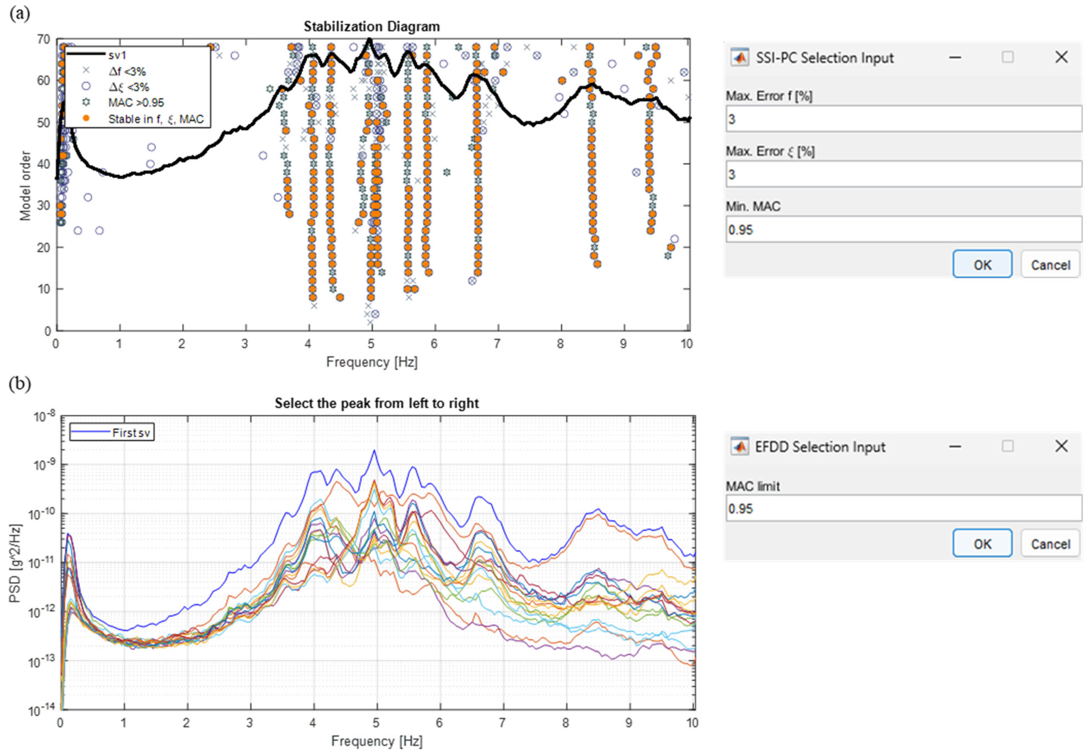
5.3.1. Manual Selection

The manual selection of modes is performed through the opening of interactive windows in which the user can select modes by mouse clicking (Figure 7). Before the opening of these windows, stability criteria between the identified solutions, which vary between time and frequency domain methods, have to be defined.

Considering time domain methods, these criteria are inherent to the variation of the modal parameters between solutions at successive model orders, and they are calculated between the poles of the stabilization diagram. In more detail, the maximum percentage variations in frequency and damping must be defined, as well as the minimum MAC threshold (defined between 0 and 1). From the authors’ experience, reasonable values to obtain a good mode selection could be set at 3% for frequency and damping differences, together with an MAC threshold of at least 0.95. For a clearer understanding, each of these criteria is represented by a different symbol in the representation of the stable pole in the stabilization diagram (cross, circle, and star); if all these conditions are satisfied, the stable pole is represented with an orange circle (Figure 7a), indicating a possible solution of the system. Poles that are not stable in any characteristic are not drawn. Solutions characterized by negative damping are automatically eliminated in the construction of the stabilization diagram as they are deemed to be unrealistic. A mode is manually selected by clicking in one of the solutions of a dot column, which is a candidate for a possible system solution. For the frequency domain method, only the MAC threshold must be defined. The relevant interactive window allows showing both the PSDs of all recordings and their first SV, as depicted in Figure 7b. Here, modes are selected by the peak-picking method.

Considering a dynamic test on the building (Figure 7), it is evident that the spectra (both PSDs and first SV) show peaks around 4 and 7 Hz, as well as in correspondence with about 8.5 and 9.5 Hz. However, these peaks are not well defined or clearly distinguishable from one another; as a result, the mode selection via the frequency domain method may not be so straightforward and may require some attempts (perhaps even many) before arriving at the choice of the final solutions. Contrarily, in this example, the method in the time domain allows for a clearer identification of eight stable modes.

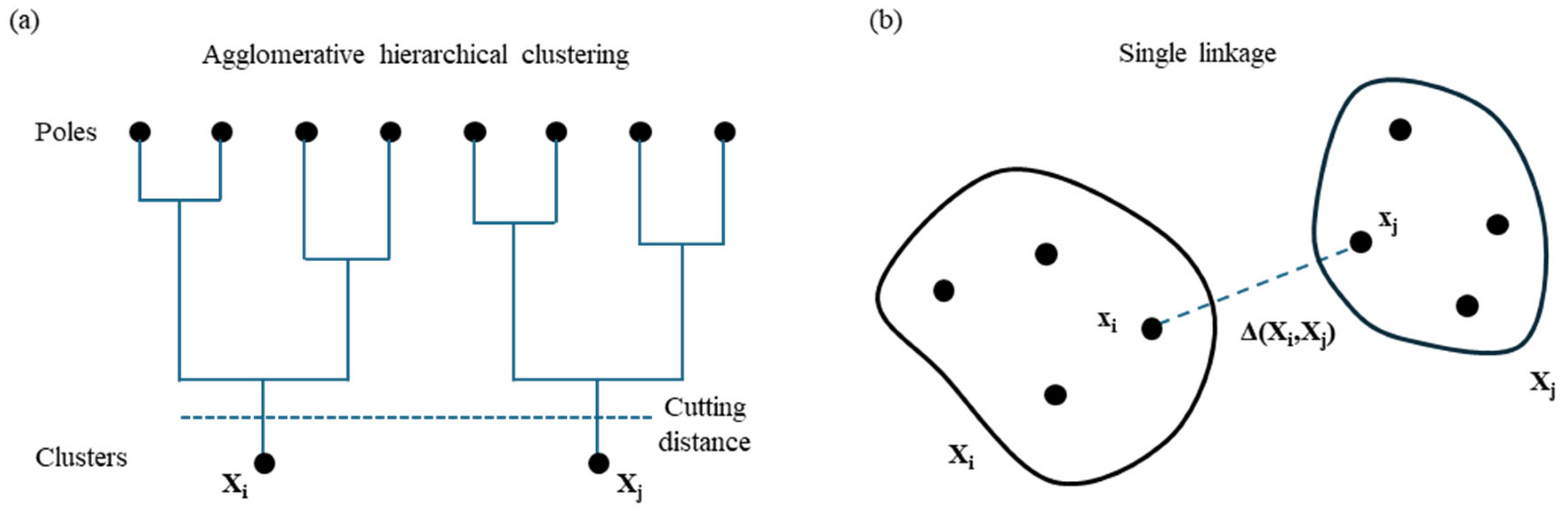
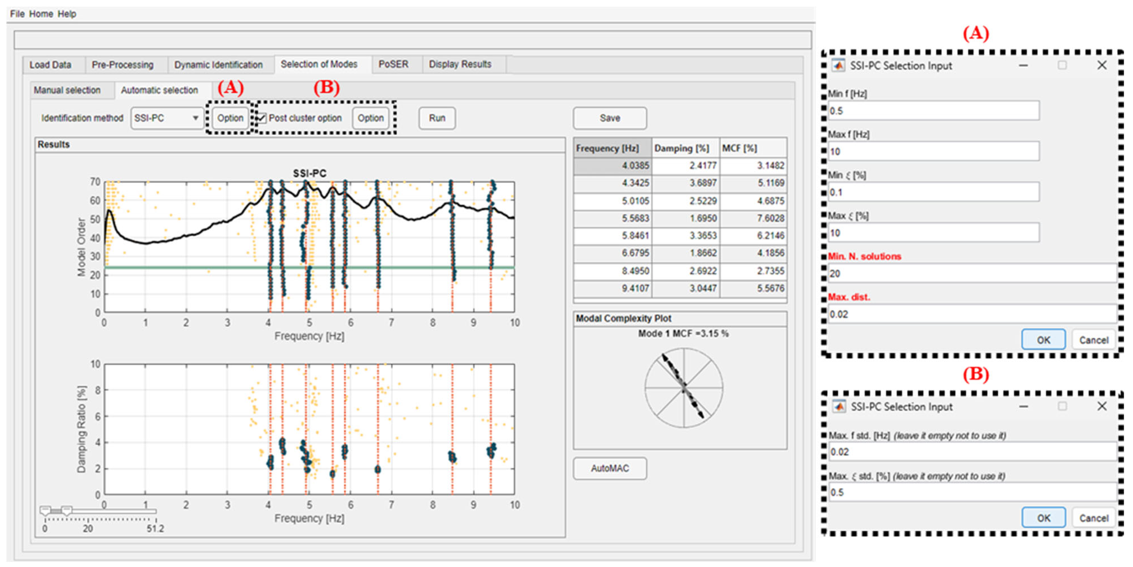
5.3.2. Automatic Selection

The automatic mode selection is implemented for time domain methods through the use of automatic procedures using clustering algorithms. An optional but very useful initial cleaning of the stabilization diagram is recommended by setting frequency and damping ratios thresholds to eliminate solutions (poles) that are outside the frequency range of interest (minimum and maximum frequency values are defined) and cannot be physically meaningful (e.g., very high or negative values of damping ratios). This preliminary step results in a clearer stabilization diagram and reduces the number of unstable poles. This option is completely customizable by the user and configures itself as a strength of this new software.

Next, mode selection is carried out to differentiate real modes from spurious ones. An effective approach to automate this step in OMA is to apply cluster analysis to the results of the stabilization diagram. Cluster analysis is a method that groups elements based on shared characteristics. In the context of stabilization diagram interpretation, it helps group identified modes with similar modal properties. The DYMOS software employs agglomerative hierarchical clustering (AHC) for this purpose. AHC starts by treating each data point as an individual cluster. At each subsequent step, the two closest clusters are merged to form a new, larger cluster. This iterative process continues, progressively reducing the number of clusters while increasing their size through successive aggregations. A schematization of the implemented clustering procedure with the hierarchical tree is represented in Figure 8a. When using a hierarchical agglomerative clustering algorithm, it is essential to define two quantities: distance and linkage. The calculation of the distance between the modal parameters of two poles i and j of the stabilization diagram can be carried out using the following formulas [27]:

$$d_{i-j}={\displaystyle \frac{\left|f_i-f_j\right|}{f_j}}+\left(1-{MAC}_{i,j}\right)$$

(18)

where f_i and f_j are the frequencies of the poles. If the distance between the mode estimates is short, both estimates present similar natural frequencies and mode shapes. Therefore, they probably represent the same physical mode, and they should be included in the same cluster. As already referred, the hierarchical algorithms differ in the way the distance between already formed clusters is assumed. In the proposed software, the single linkage is used, namely, the distance between two clusters is assumed to be equal to the shortest distance between any point of one cluster and any point of the other (Figure 8b):

$$∆\left(X_i,X_j\right)=\underset{x_i\in X_i,x_j\in X_j}{\mathit{min}}d\left(x_i,x_j\right)$$

(19)

where x_i and x_j are elements belonging to cluster X_i and X_j, respectively.

The next step is the selection of the hierarchical tree cut level that consists of imposing an upper limit on the distance between any point of the same cluster (“Max dist.” in the software). The lower the distance is, the higher the number of resulting clusters is. The definition of this distance is not generalizable but depends on the case study under consideration. In fact, depending on the choice of this distance, the clustering results may considerably vary, especially if the poles are spread along the vertical at a certain frequency (quite unstable mode) or in the case of closed-space modes with similar modal shapes (where the difference in MAC is low). In order for the algorithm to select modes in the above two cases, it is advisable to adopt a high distance in the first case and a short distance in the second one. However, another parameter for the cluster selection is to define a minimum number of solutions contained within it (“Min N. solutions” in the software). Indeed, the possibility that the cluster represents a physical mode of the structure increases if the number of solutions grouped within it increases. It is suggested to adopt between 10 and 20 solutions, depending on the maximum model order selected for the identification.

At the end of the clustering, each cluster represents a mode of the system. An example of clustering results for the building case study is illustrated in Figure 9. The stabilization diagram is plotted together with the frequency–damping diagram, and the solutions grouped in different clusters are represented with dark blue dots.

Another key feature of the software is the possibility to remove clusters with high dispersions in frequency and/or damping ratios values (using the “Post cluster option”), as they generally do not represent the real modes of the structure. This is achieved by setting an upper limit to the standard deviation calculated on frequencies and/or damping ratios of the solutions within the same cluster. The software allows the selection of this option simultaneously or separately on both parameters. For instance, in the example of Figure 9, applying a standard deviation of 0.02 Hz for frequency value and 0.5% for the damping ratio value prevents the selection of the mode just below 4 Hz and one just above 5 Hz. The remaining modes have small frequency variations (the blue dot columns are almost perfectly vertical) and small damping ratio variations (whose values for each cluster are highly grouped).

The modal parameters (i.e., frequency, damping ratio, and mode shape) of each selected mode after the clustering correspond to those of the solution belonging to each cluster and relevant to the lowest model order that is common to all clusters (indicated by a horizontal green line in the stabilization diagram). In the case where a common model order cannot be found, the selected modal parameters correspond to the solution with the lowest MCF.

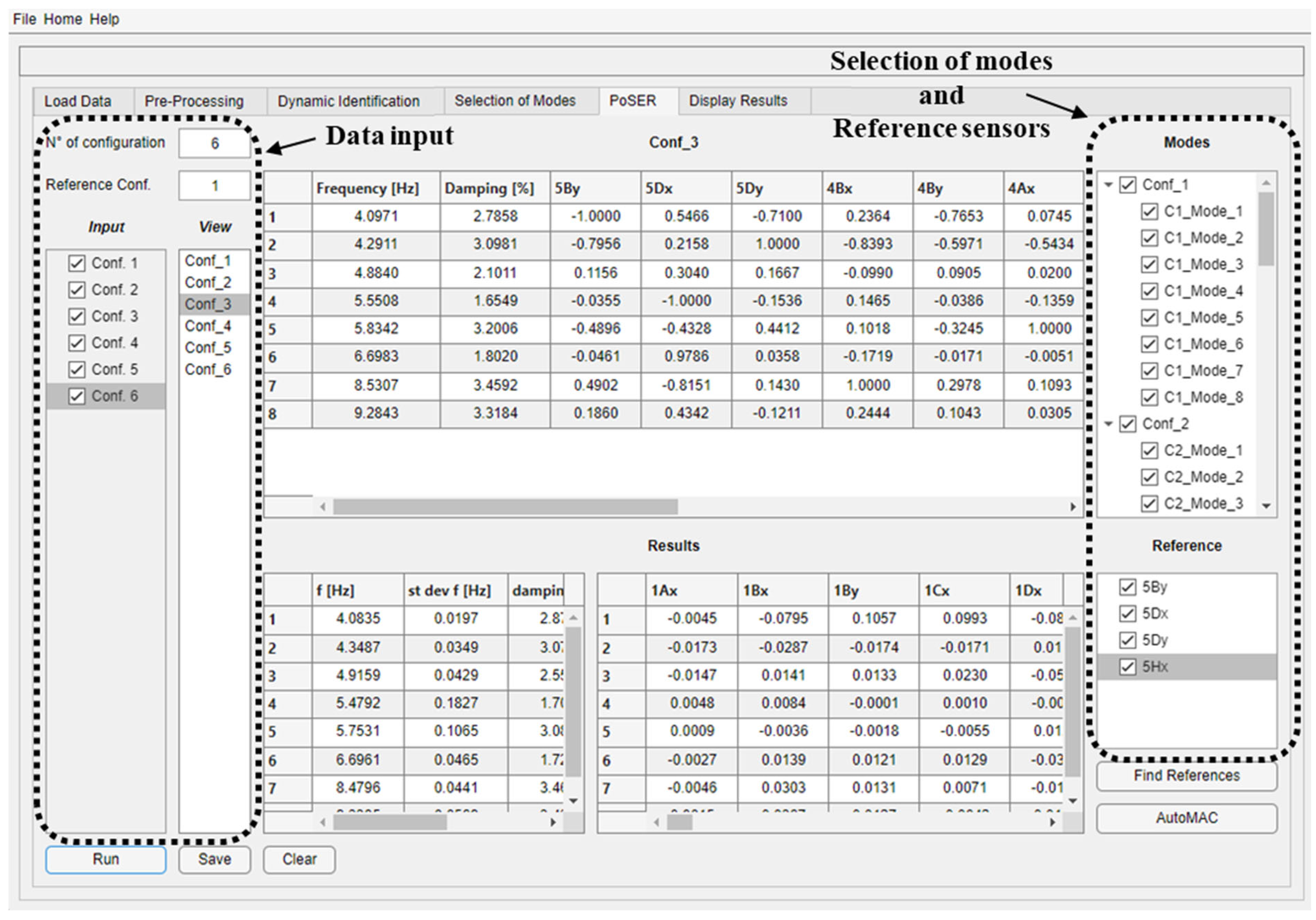
6. Module for Merging Results from Multiple Test Set-Ups

AVTs of civil engineering structures typically require measuring the structure response at numerous locations, ensuring sufficient spatial resolution to effectively catch all modes and accurately characterize mode shapes. Often, the limited number of available sensors or acquisition channels imposes the development of several test set-up, keeping some sensors always in the same position (reference sensors) and moving others (moving sensors) until the whole structure is covered. In these cases, the dynamic identification of a structure involves the use of several non-simultaneous measurement configurations, and the identifications separately performed on each of them can be put together by using reference sensors and adopting different merging techniques. The presented software allows this to be performed using the Post Separate Estimation Re-scaling (PoSER) technique [28]. Typically, the outcomes of a specific configuration where all pertinent modes of the structure are successfully identified serve as a benchmark, referred to as set-up k. Subsequently, results of the other j-th configurations are paired to the reference ones (k) on the basis of frequencies and mode shapes similarities. Thus, for each i-th mode, the modal displacements (collected in the vector $\mathit{\varphi }$) are scaled by a factor $\alpha$ that minimizes the differences with the components of the reference sensors in the reference configuration:

$${\mathit{\varphi }}_i^{j\to k}={\alpha }_i^{j\to k}·{\mathit{\varphi }}_i^j$$

(20)

with

$${\alpha }_i^{j\to k}={\displaystyle \frac{{\left({\mathit{\varphi }}_i^{j,ref}\right)}^H·\left({\mathit{\varphi }}_i^{k,ref}\right)}{{\left({\mathit{\varphi }}_i^{j,ref}\right)}^H·\left({\mathit{\varphi }}_i^{j,ref}\right)}}$$

(21)

where ref identifies the reference sensor modal displacements.

The “PoSER” module of the software (Figure 10) requires loading multiple modal identification results in a predefined format, which matches the format used for saving results in the “Selection of modes” module. Once all configurations are loaded, it is possible to select via a check box on the right-hand side the modes to be considered for each of them, and that must be common to all configurations. The software automatically recognizes the sensors common to all the configurations, i.e., those used as a reference. In addition, it is possible to use a reduced number of reference sensors by simply selecting via check boxes those that are deemed necessary. At the end of the procedure, a table collecting the scaled mode shape displacements can be saved as an .xlsx format file.

To dynamically test both case studies, many sensor configurations (and non-contemporary AVTs) were performed due to the size and complexity of the structures. Reference sensors were always left in the same positions (highlighted in red in Figure 11). For the building case study, six sensor configurations were adopted, as shown in Figure 11a. The same sensor layout was used for all the six floors: for each block, three sensors per floor were used because the in-plane rigid assumption of floors was assumed realistic. Moreover, two sensors per block located at the fifth level were used as a reference. Considering the bridge, three sensors per cross-section were employed to capture the displacement components of bending, torsional, and transverse modes of the deck (Figure 11b). All cross-sections where stay cables are connected to the deck were measured in order to obtain refined modal deformations. Four sensor configurations were necessary to test the whole bridge, and for all of them, two cross-sections approximatively at the mid-length of the bridge were left as a reference. Additionally, in one of these reference sections, a further sensor was positioned, measuring in the longitudinal direction.

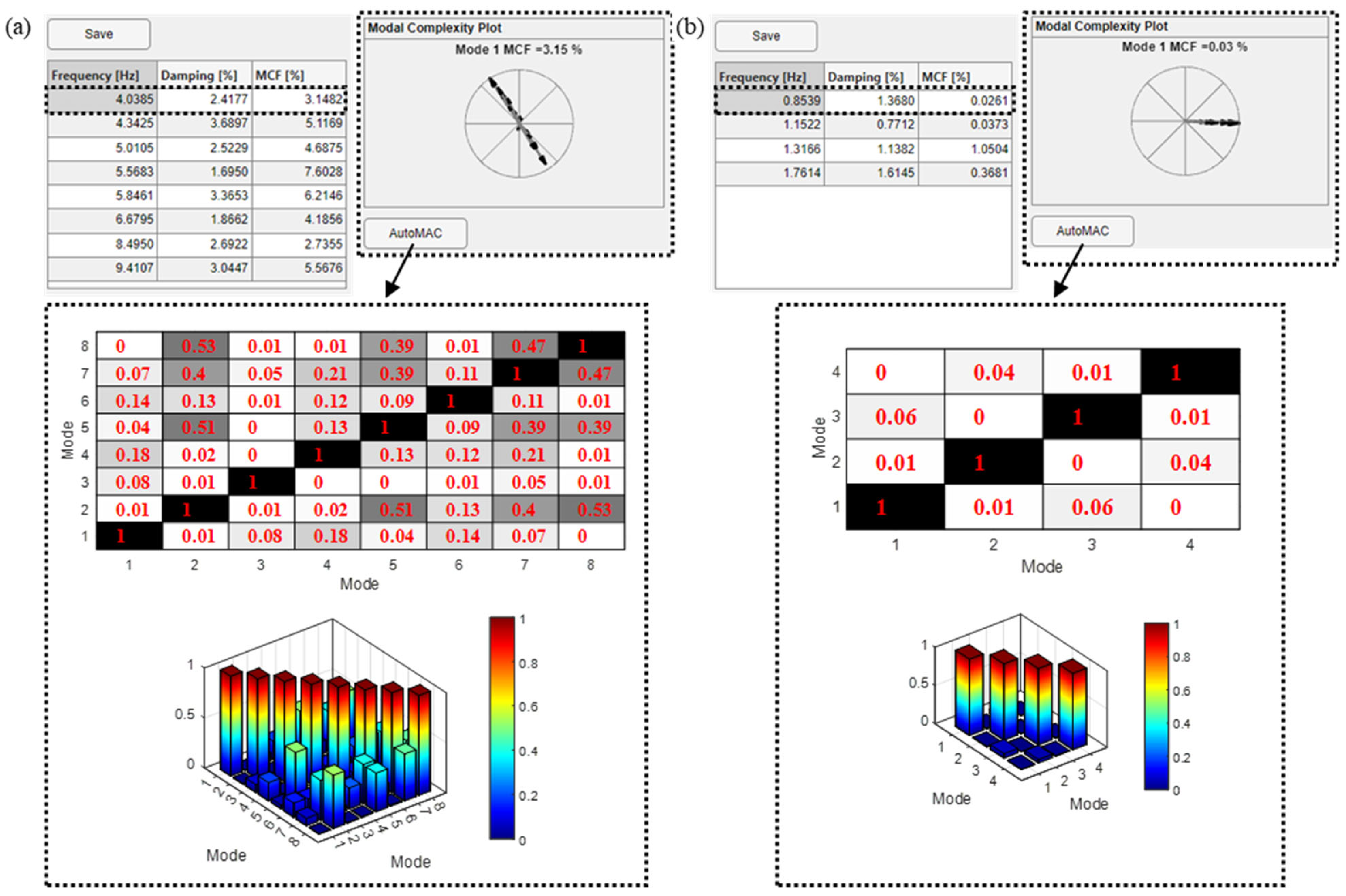
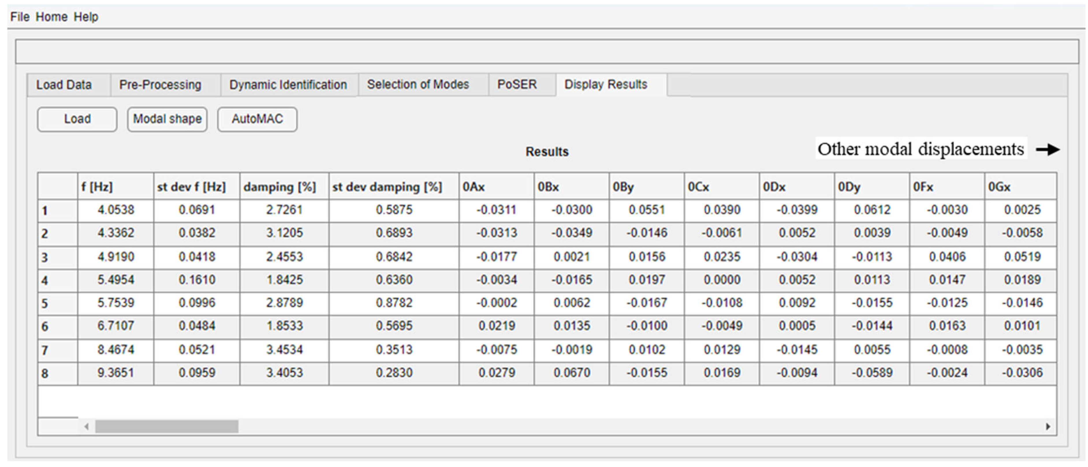
7. Module to Display Results

The “Display Results” module is one of the strengths of DYMOS software as it has the great advantage of using CAD drawings (i.e., files in .dxf format) as geometry input data, making the construction of the geometric model and measurement grid much simpler, faster, and intuitive, thus guaranteeing a simple yet detailed visualization of mode shapes. At the beginning, the loading of modal parameters saved either at the end of the mode selection procedure (in case of a single test configuration) or after the PoSER execution is required. A table summarizing the identified modal parameters is shown (Figure 12), which, in the case of PoSER results, contains the average values of frequencies and damping ratios values of the different modes among all configurations, their standard deviation to quantify the scattering of these modal parameters during the whole test period (“st. dev. f” and “st. dev. damping”), and all the modal displacements of all sensors correctly scaled. The variations of modal parameters of different configurations could be due to the uncertainty in the adopted identification method as well as due to the influence of environmental (e.g., temperature) and operational factors (e.g., anthropic activities within or close to the structure) that may vary during the test operations. Then, the loading of the geometric model of the structure is required as well. After that, the mode shapes are plotted thanks to an interactive window that allows the selection of the mode to be displayed and allows for the definition of the mode shape scaling factor. The geometrical CAD model must be differently created as a function of the tested structural typology. The software has implemented two tools suitable for buildings and bridges with all types of geometries.

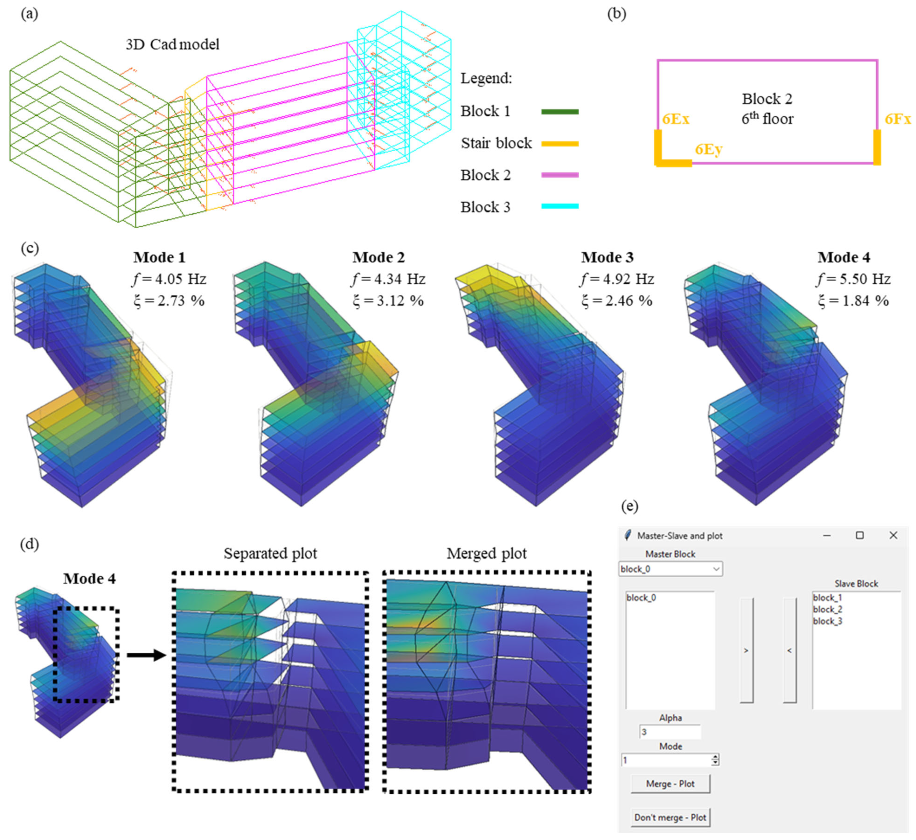
7.1. Tool to Display Mode Shapes for Buildings

This tool makes it possible to visualize the modal shapes of buildings of any geometry, even those composed of multiple blocks separated by structural joints. The initial geometrical model is a 3D model drawn in a CAD environment, where the contour of each building block is drawn with line elements. The representation of the modal shapes of each floor is based on the rigid plane assumption, i.e., the kinematics of the floor is described by three DOFs (two translations and one rotation in the plane). Therefore, if the building has an articulated plan shape (e.g., L-shape), it is necessary to create a spatial model subdivided into several simple blocks (preferably rectangular), in which the rigid plane assumption can be considered valid. The division into multiple blocks is also necessary if the buildings are separated from each other by structural joints. The contours of the various blocks must be drawn in continuity, i.e., they must have one or more sides in common, even in the case of buildings separated by structural joints. For the building case study, the four bodies are divided into different blocks drawn in contact, as illustrated in Figure 13a. The floors are drawn with surfaces with three or four edges; if the floor has an articulated shape, it can be subdivided into several simple surfaces. On each floor of each block, it is necessary to have two measurement points in the plane, one bi-axial and one mono-axial, the latter being necessary for the calculation of the floor rotation. The measuring directions are represented with positively oriented lines according to the measuring sensor direction. Each measurement axis must be associated with a text recalling the name of the sensor axis (the same name assigned in the “Load Data” module). The insertion point of the text must coincide with the end of the line representing the corresponding measurement axis (Figure 13b). All line elements (both structure and sensor directions), surfaces, and text must belong to the same layer, which is different for each of the considered blocks. However, the color of the lines representing the measurement directions must differ from that of the layer to which they belong. The latter is a software requirement for the correct recognition of these elements.

Starting from the modal displacements provided as input, the software enables the visualization of the mode shapes for the various blocks of the building. In the plot, the undeformed shape is also represented with light grey lines to support the mode shape interpretation. Furthermore, the display tool permits the visualization of mode shapes in two different ways. The first option allows the blocks to be separately considered; therefore, the modal deformations are also separately displayed. This option is useful for representing mode shapes of adjacent buildings separated by structural joints. The mode shapes of the first four modes of the building case study are represented by using this option in Figure 13c. The second display option involves joining the edges of separate blocks to form a continuous modal deformation. This second option can be used in the case of buildings with articulated plan shapes but composed by a unique body. In this second case, in order to connect the mode shapes of several blocks, it is necessary to define which of them is the master block, to which the deformations of the slave blocks will be connected. For the sake of clearance, an example of visualization of the two-plot methodology is represented in Figure 13d for the fourth mode shape of the building case study.

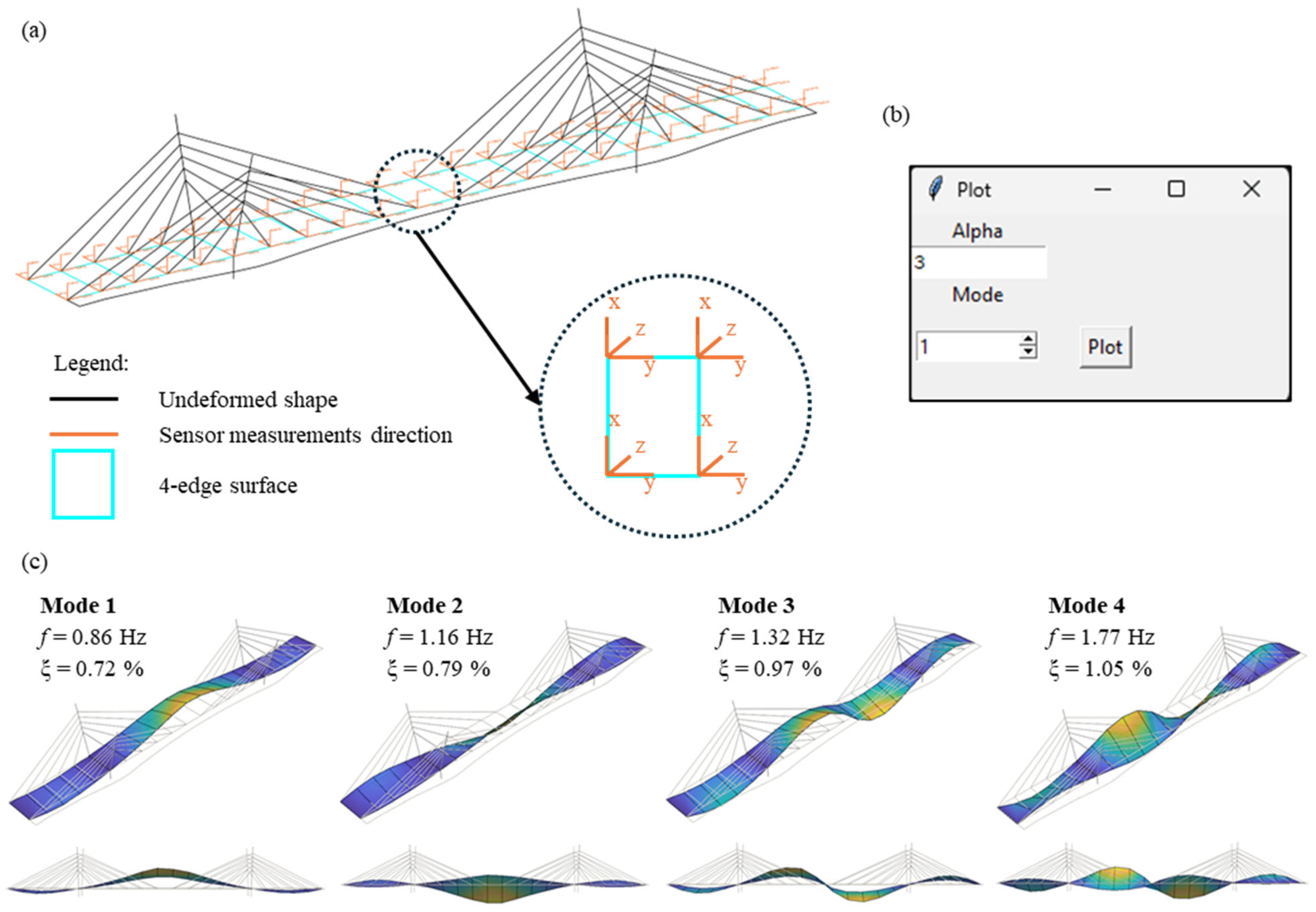
7.2. Tool to Display Mode Shapes for Bridges

This tool makes it possible to visualize the mode shapes of the deck of any type of bridge (e.g., simply supported spans, continuous spans, arch bridges, etc.). The initial geometric model is once again a 3D CAD model (Figure 14a). The bridge deck must be divided into four-edge surfaces drawn in continuity and with a common edge in case bridges with a continuous deck, or separated in case of bridges with a simply supported span deck. The software algorithm deforms each surface according to the 3D displacements of each of the four vertices. Additionally, it is possible to draw the other components of the bridge (e.g., piers, stays, pylons, etc.) with line elements. The latter remain undeformed and compose the shaded undeformed shape in background to the mode shape of the deck. On each edge of the deck surfaces, four tri-axial measuring points must be drawn, two must be horizontal and orthogonal in the plane, and one must be vertical. The measuring directions are represented with positively oriented lines, as for buildings. Each measurement axis must be associated with a text recalling the name of the sensor axis (the same name assigned in the “Load Data” form). The insertion point of the text must coincide with the end of the line representing the corresponding measurement axis.

In the event that four tri-axial points have not been measured for each surface, these must be represented with fictitious names. The software automatically recognizes that these vertices do not correspond to measured points and assigns them zero displacements in the corresponding directions. All lines, surfaces, and text elements must belong to the same layer. The color of the lines of the measurement directions must be different from that of the layer to which they belong. In Figure 14b, the mode shapes of the first four modes identified for the bridge case study are represented.

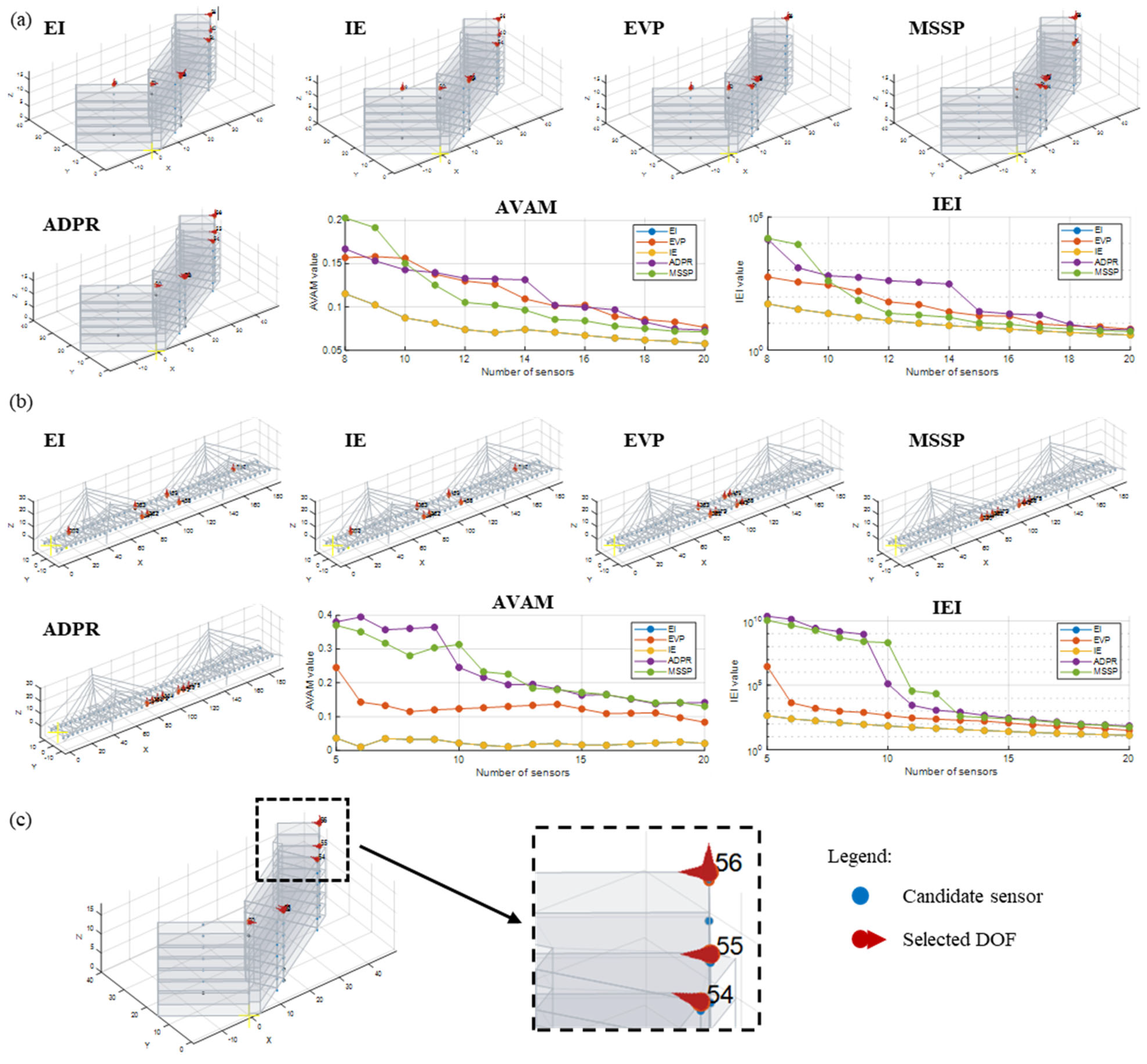
8. Module for the OSP

The second task of the software is dedicated to the OSP. To the best of the authors’ knowledge, it is the first time a OSP module has been integrated in an OMA software, improving its usability and usefulness. This module allows for the execution of OSP analyses, adopting as input either numerical or experimental data. The former can be obtained from a numerical model of the structure, while the latter from OMA. In both cases, the input (in terms of frequencies and modal displacements of selected/all joints) is provided by using standard .xlsx format files in which data must be prepared following a standard format and layout. In addition, numerical data can be directly loaded from the software if the CSI SAP2000 software [29] is used. Indeed, a SAP-MATLAB toolbox [30] is used to create this module that allows for communication with the finite element model (FEM) developed in SAP2000 and the DYMOS software. Only a brief description of the OSP module is given in this manuscript (Figure 15) as this is an up-to-date version of the MATLAB software presented in the work of Nicoletti et al. [31], where the reader may find all the relevant details. Moreover, this paper does not provide a detailed discussion of the adopted OSP methods and their potential and limitations in structural engineering applications, as this topic is addressed in another work already published by the authors [32]. In this work, the use of this module is described with reference to the two case studies.

The OSP module implements five well-known OSP methods from the literature: effective independence (EI), information entropy (IE), eigenvalue vector product (EVP), mode shape summation plot (MSSP), and average driving point residue (ADPR). The selected DOFs at the end of the OSP analysis are shown in both tabular and graphic form. For graphic visualization, the module allows for the background profile of the structure to be displayed (loaded via files in .dxf format, the same used in the “Display Results” module described in the Section 7), with the selected nodes and measurement directions being highlighted by red arrows and identified with their identification numbers from the imported node list. The effectiveness of the OSP-generated configurations is quantitatively assessed using metrics that gauge sensor configuration robustness in identifying mode shapes. Two metrics are implemented, the average value of the off-diagonal terms of the AutoMAC matrix (AVAM) and the information entropy index (IEI). AVAM measures mode shape orthogonality (0 to 1, good to bad results), as well as IEI (the target is to obtain results close to 1). Graphs showing metric changes with the number of sensors are also provided, assisting in determining the optimal number and position of sensor for effectively capturing the dynamic behavior of the structure.

This module of the software is used to find the best sensor configurations to dynamically identify the two case studies investigated in this work. The OSP analyses are performed starting from the experimental data, i.e., by importing the identified modal displacements (after the PoSER application) of the DOFs tested during AVTs. Thus, the manual import option is used as experimental data are considered. A totality of 84 DOFs for the building and 60 for the bridge are considered. Few input data must be defined before performing the analyses: the number of modes to be considered and that need to be clearly identifiable by the reduced set of sensors (eight modes for the building and four for the bridge), the minimum number of sensors to employ (eight for the building and seven for the bridge), and also the maximum one (twenty for both case studies). The latter is required to build metric graphs and to investigate the OSP method performance when the number of sensors increases, aiding finding the right number of sensors to be employed. Instead, the minimum number of sensors should be set at least equal to the number of modes to be identified. A low number of sensors can lead to difficulties in clearly identifying the mode shapes and to the occurrence of the so-called spatial aliasing problem. For the bridge, a greater number of sensors with respect to the minimum required (seven DOFs instead of four) is considered as this bridge is now monitored with this number of sensors [33]; hence, this OSP analysis is used as a confirmation of the correctness of the actual sensor position. The results of the OSP analyses are reported in Figure 16. For each case study, the software allows the sensor layout to be plotted separately for each OSP method. This plot is also interactive, permitting one to zoom and rotate the structure to easily read the results. For the building, all methods select joints (DOFs) at the higher level because they are the ones that experienced the higher modal displacements. For the bridge, the EI and IE methods select joints spread along the bridge deck, while the other methods select joints mainly located at the mid-span. Obviously, the solutions of EI and IE seem to be the best ones as they allow for a better identification of the higher modes too. This is also clear from the metric graph of the bridge as both AVAM and IEI do not show variation for EI and IE by increasing the number of DOFs. The same can be said for the building, even if in this case all metrics improve (namely, decrease) if the sensor number increases, for instance up to 14 sensors.

9. Conclusions

This work introduced the new DYMOS software for the dynamic identification of structures from ambient noise recordings. DYMOS incorporates a collection of state-of-the-art algorithms and tools for vibration-based modal identification and OSP of structures, organized into separate modules with customizable analysis parameters. This approach aims to bridge the gap between professional practice and research needs. The article aimed to describe the DYMOS software and demonstrate its potential for OMA and OSP in civil engineering structures. To achieve this, two real case studies (recently dynamically tested) have been identified and analyzed using the proposed software. The manuscript thoroughly explains all the steps required for the dynamic identification of the two case studies and describes the main functionalities of the software. Pre-processing techniques are applied to the dataset from both case studies, as well as all the identification methods available in the software are used to identify the dynamic behavior of the case studies. The parameters adopted for the OMA and for the mode selection of each case study are stated, providing useful support when dealing with the dynamic identification of such structures. Finally, OSP analyses are performed starting from the experimental results and with the target to obtain the best sensor configurations that could be employed in a dynamic SHM of these structures.

DYMOS software offers several strengths that differentiate it from other similar tools. At first, to the best of the authors’ knowledge, it is the first software containing together one part for performing the OMA and another one for the OSP. These two tasks are closely interconnected as the OSP is a fundamental component for conducting accurate dynamic tests and the corresponding OMA. Secondly, a new graphical tool is implemented for visualizing results in both buildings and bridges. It simplifies model construction by using CAD drawings as input, making the process faster, more intuitive, and efficient. DYMOS also offers other several key features, including a separate mode selection module for clear and customizable mode selection without re-running system identification, reducing computational effort. It supports both manual and guided mode selection, making it accessible to all users. Input parameters for mode identification and clustering are fully customizable, making it also suitable for research purposes. Additionally, it removes clusters with high dispersion in frequency or damping, ensuring accurate mode identification.

In conclusion, the DYMOS software marks a significant advance in the dynamic identification of structures, offering customizable modules that are both suitable for practitioners and researchers. Its unique features, together with its intuitive graphical user interface, streamline the analysis process. The software’s successful application in real case studies highlights its effectiveness and versatility in the civil engineering field. A future target of the authors is to update the software with an additional module for the management and analysis of data collected from both dynamic and static SHM systems installed in civil engineering structures, aiming at facilitating the assessment and management of structures and infrastructure.

References

1. Rainieri, C.; Fabbrocino, G. Development and validation of an automated operational modal analysis algorithm for vibration-based monitoring and tensile load estimation. Mech. Syst. Signal Process. 2015, 60, 512–534. [Google Scholar] [CrossRef]
2. Amador, S.D.R.; Brincker, R. The new Subspace-based poly-reference Complex Frequency (S-pCF) for robust frequency-domain modal parameter estimation. Meas. J. Int. Meas. Confed. 2024, 225, 113995. [Google Scholar] [CrossRef]
3. Maes, K.; Van Meerbeeck, L.; Reynders, E.P.B.; Lombaert, G. Validation of vibration-based structural health monitoring on retrofitted railway bridge KW51. Mech. Syst. Signal Process. 2022, 165, 108380. [Google Scholar] [CrossRef]
4. Giordano, P.F.; Quqa, S.; Limongelli, M.P. The value of monitoring a structural health monitoring system. Struct. Saf. 2023, 100, 102280. [Google Scholar] [CrossRef]
5. Oyarzo-Vera, C.; Ingham, J.; Chouw, N. Vibration-based damage identification of an unreinforced masonry house model. Adv. Struct. Eng. 2017, 20, 331–351. [Google Scholar] [CrossRef]
6. Pereira, S.; Magalhães, F.; Gomes, J.P.; Cunha, Á. Modal tracking under large environmental influence. J. Civ. Struct. Health Monit. 2022, 12, 179–190. [Google Scholar] [CrossRef]
7. Ventura, C.E.; Schuster, N.D. Structural dynamic properties of a reinforced concrete high-rise building during construction. Can. J. Civ. Eng. 1996, 23, 950–972. [Google Scholar] [CrossRef]
8. Anastasopoulos, D.; De Roeck, G.; Reynders, E.P.B. One-year operational modal analysis of a steel bridge from high-resolution macrostrain monitoring: Influence of temperature vs. retrofitting. Mech. Syst. Signal Process. 2021, 161, 107951. [Google Scholar] [CrossRef]
9. Pereira, S.; Magalhães, F.; Gomes, J.P.; Cunha, Á.; Lemos, J.V. Vibration-based damage detection of a concrete arch dam. Eng. Struct. 2021, 235, 112032. [Google Scholar] [CrossRef]
10. Diord, S.; Magalhães, F.; Cunha, A.; Caetano, E. High spatial resolution modal identification of a stadium suspension roof: Assessment of the estimates uncertainty and of modal contributions. Eng. Struct. 2017, 135, 117–135. [Google Scholar] [CrossRef]
11. Borlenghi, P.; Gentile, C.; D’Angelo, M.; Ballio, F. Long-term monitoring of a masonry arch bridge to evaluate scour effects. Constr. Build. Mater. 2024, 411, 134580. [Google Scholar] [CrossRef]
12. Arezzo, D.; Quarchioni, S.; Nicoletti, V.; Carbonari, S.; Gara, F.; Leonardo, C.; Leoni, G. SHM of historical buildings: The case study of Santa Maria in Via church in Camerino (Italy). Procedia Struct. Integr. 2023, 44, 2098–2105. [Google Scholar] [CrossRef]
13. Diaferio, M.; Foti, D.; Giannoccaro, N.I.; Ivorra, S. Model updating based on the dynamic identification of a baroque bell tower. Int. J. Saf. Secur. Eng. 2017, 7, 519–531. [Google Scholar] [CrossRef]
14. Ierimonti, L.; Cavalagli, N.; Venanzi, I.; García-Macías, E.; Ubertini, F. A transfer Bayesian learning methodology for structural health monitoring of monumental structures. Eng. Struct. 2021, 247, 113089. [Google Scholar] [CrossRef]
15. Innocenzi, R.D.; Nicoletti, V.; Arezzo, D.; Carbonari, S.; Gara, F.; Dezi, L. A Good Practice for the Proof Testing of Cable-Stayed Bridges. Appl. Sci. 2022, 12, 3547. [Google Scholar] [CrossRef]
16. Nicoletti, V.; Arezzo, D.; Carbonari, S.; Gara, F. Dynamic monitoring of buildings as a diagnostic tool during construction phases. J. Build. Eng. 2022, 46, 103764. [Google Scholar] [CrossRef]
17. Wah, W.S.L.; Chen, Y.-T.; Roberts, G.W.; Elamin, A. Separating damage from environmental effects affecting civil structures for near real-time damage detection. Struct. Health Monit. 2018, 17, 850–868. [Google Scholar] [CrossRef]
18. Ubertini, F.; Cavalagli, N.; Kita, A.; Comanducci, G. Assessment of a monumental masonry bell-tower after 2016 Central Italy seismic sequence by long-term SHM. Bull. Earthq. Eng. 2018, 16, 775–801. [Google Scholar] [CrossRef]
19. MOVA/MOSS: Two integrated software solutions for comprehensive Structural Health Monitoring of structures. Mech. Syst. Signal Process. 2020, 143, 106830. [CrossRef]
20. Pasca, D.P.; Aloisio, A.; Rosso, M.M.; Sotiropoulos, S. PyOMA and PyOMA_GUI: A Python module and software for Operational Modal Analysis. SoftwareX 2022, 20, 101216. [Google Scholar] [CrossRef]
21. Peeters, B. System Identification and Damage Detection in Civil Engineering; KU Leuven: Leuven, Belgium, 2000. [Google Scholar]
22. Brincker, R. Some Elements of Operational Modal Analysis. Shock Vib. 2014, 2014, 325839. [Google Scholar] [CrossRef]
23. Van Overschee, P.; De Moor, B. Subspace identification for linear systems. In Theory, Implementation, Applications; Springer Science & Business Media: Berlin/Heidelberg, Germany, 1996; Volume 14, p. 254. [Google Scholar] [CrossRef]
24. Brincker, R.; Ventura, C.; Andersen, P. Damping estimation by Frequency Domain Decomposition. In Proceedings of the International Modal Analysis Conference, Kissimmee, FL, USA, 5–8 February 2001. [Google Scholar]
25. Sevim, B.; Bayraktar, A.; Altunişik, A.C.; Adanur, S.; Akköse, M. Modal Parameter Identification of a Prototype Arch Dam Using Enhanced Frequency Domain Decomposition and Stochastic Subspace Identification Techniques. J. Test. Eval. 2010, 38, 588–597. [Google Scholar] [CrossRef]
26. Chopra, A.K. Dynamics of Structures: Theory and Applications to Earthquake Engineering; Pearson: London, UK, 2017. [Google Scholar]
27. Magalhães, F.; Cunha, Á.; Caetano, E. Online automatic identification of the modal parameters of a long span arch bridge. Mech. Syst. Signal Process. 2009, 23, 316–329. [Google Scholar] [CrossRef]
28. Parloo, E. Application of Frequency-Domain System Identification Techniques in the Field of Operational Modal Analysis. Ph.D. Thesis, Vrije Universiteit Brussel, Ixelles, Belgium, 2003. [Google Scholar]
29. SAP2000|STRUCTURAL ANALYSIS AND DESIGN. Available online: https://www.csiamerica.com/products/sap2000 (accessed on 17 June 2024).
30. SAP+MATLAB. 2024. Available online: https://it.mathworks.com/matlabcentral/fileexchange/79271-sap-matlab (accessed on 17 June 2025).
31. Nicoletti, V.; Quarchioni, S.; Martini, R.; Gara, F.; Gaile, L.; Singh, H. A Novel Software Tool for the Optimal Sensor Placement in Civil Engineering Structures. In Proceedings of the 10th International Operational Modal Analysis Conference (IOMAC 2024), Naples, Italy, 22–24 May 2024; Rainieri, C., Gentile, C., Aenlle López, M., Eds.; Lecture Notes in Civil Engineering; Springer Nature: Cham, Switzerland, 2024; Volume 514, pp. 448–455. [Google Scholar] [CrossRef]
32. Nicoletti, V.; Quarchioni, S.; Amico, L.; Gara, F. Assessment of different optimal sensor placement methods for dynamic monitoring of civil structures and infrastructures. Struct. Infrastruct. Eng. 2024. [Google Scholar] [CrossRef]
33. Nicoletti, V.; Amico, L.; Martini, R.; Carbonari, S.; Gara, F.; Dezi, F. The Monitoring System of the New Filomena Delli Castelli Cable-Stayed Bridge. In Experimental Vibration Analysis for Civil Engineering Structures 2023; Limongelli, M.P., Giordano, P.F., Quqa, S., Gentile, C., Cigada, A., Eds.; Lecture Notes in Civil Engineering; Springer Nature: Cham, Switzerland, 2023; Volume 432, pp. 401–411. [Google Scholar] [CrossRef]
Figure 1. Software main screen and description of module contents.
Buildings 15 02194 g001
Figure 2. Case studies adopted for the DYMOS software testing and validation: (a) 4-block building; (b) cable-stayed bridge.
Buildings 15 02194 g002
Figure 3. Example of the “Load Data” module usage for a dynamic test performed on the building case study.
Buildings 15 02194 g003
Figure 4. Example of the “Pre-Processing” module usage for a dynamic test performed on the building case study.
Buildings 15 02194 g004
Figure 5. “Dynamic Identification” module and example of definition of the identification parameters for both case studies.
Buildings 15 02194 g005
Figure 6. Results for the identification of the two case studies: (a) the building; (b) the bridge.
Buildings 15 02194 g006
Figure 7. Interactive windows for the manual selection of modes: (a) time domain methods; (b) frequency domain method.
Buildings 15 02194 g007
Figure 8. Schematization of the clustering procedure: (a) hierarchical tree for the grouping of solutions; (b) assumed distance for the cluster definition (single linkage).
Buildings 15 02194 g008
Figure 9. Example of the software tab for the automatic selection of modes from an AVT on the building.
Buildings 15 02194 g009
Figure 10. DYMOS module for the PoSER module.
Buildings 15 02194 g010
Figure 11. Sensor layouts and configurations to dynamically test the case studies: (a) the building; (b) the bridge.
Buildings 15 02194 g011
Figure 12. Example of table of results for the building case study obtained after the PoSER module and loaded in the “Display Results” module.
Buildings 15 02194 g012
Figure 13. Tool to display the mode shapes of buildings: (a) initial 3D CAD model; (b) minimum sensor layout for each block; (c) visualization of the first 4 mode shapes for the building case study; (d) differences in the visualization of mode shapes (separated and merged plot); (e) interactive window for the mode shape plot of buildings.
Buildings 15 02194 g013
Figure 14. Tool to display mode shapes of bridges: (a) initial 3D CAD model; (b) interactive window for the mode shape plot of bridges; (c) visualization of the first 4 mode shapes for the bridge case study.
Buildings 15 02194 g014
Figure 15. DYMOS module for the OSP.
Buildings 15 02194 g015
Figure 16. OSP results for the case studies: (a) the building; (b) the bridge; (c) enlargement for the visualization of selected DOFs.
Buildings 15 02194 g016
Disclaimer/Publisher’s Note: The statements, opinions and data contained in all publications are solely those of the individual author(s) and contributor(s) and not of MDPI and/or the editor(s). MDPI and/or the editor(s) disclaim responsibility for any injury to people or property resulting from any ideas, methods, instructions or products referred to in the content.