A Study of the Fractal Bending Behavior of Timoshenko Beams Using a Fourth-Order Single Equation

Abstract

In this paper a new generalized fractal equation for studying the behaviour of self-similar beams using the Timoshenko beam theory is introduced. This equation is established in fractal dimensions by applying the concept of fractal continuum calculus $F^{\alpha }$-CC introduced recently by Balankin and Elizarraraz in order to study engineering phenomena in complex bodies. Ultimately, the achieved formulation is a fourth-order fractal single equation generated by superposing a shear deformation on an Euler–Bernoulli beam. A mapping of the Timoshenko principle onto self-similar beams in the integer space into a corresponding principle for fractal continuum space is formulated employing local fractional differential operators. Consequently, the single equation that describes the stress/strain of a fractal Timoshenko beam is solved, which is simple, exact, and algorithmic as an alternative description of the fractal bending of beams. Therefore, the elastic curve function and rotation function can be described. Illustrative examples of classical beams are presented and show both the benefits and the efficiency of the suggested model.

1. Introduction

Fractal geometry is an alternative mathematical framework thanks to its capability to describe natural objects as broccoli, clouds, mountains, and coastlines, among others [1]. The use of fractal geometry has been widely implemented in several areas of science and technology such as hydrology [2], mechanics [3,4], medicine [5], civil engineering [6,7], and so forth.

Many materials and man-made objects possess a complicated architecture with self-similar properties, which are known as fractals. The functions defined in such domains are discontinuous or are not differentiable in some points [8]. So, physical phenomena occurring on a fractal set cannot be described by applying the conventional calculus. Consequently, different methodologies have been introduced to overcome this drawback, for example, fractional [9], fractal [10], and fractal continuum calculus [11,12,13].

In this regard, the above approaches have been used for beam theory in structural engineering in order to describe the stress and strain presented in beams with complex, heterogeneous, or nano geometries.

Modified fractional equations of the original Euler–Bernoulli beam were suggested in references [14,15], and fractional Timoshenko beam theory was introduced in [16], whose formulations use a real-line measure, which is not a fractal measure, such as in classical Timoshenko beam theory [17]. Afterward, generalizations of these theories were introduced using fractal continuum calculus [18]. They employ non-standard measures; the fractal measure has a more complete description of the relevant engineering behavior because the fractal formulations include the geometry and fractal topology of self-similar beams under study.

In this work, the fractal continuum approach is used, specifically, fractal continuum calculus $F^{\alpha }$-CC [12,13], which consists in replacing the fractal body F with a continuum body $F^{\alpha }$ [19] and to characterize it by a set of local fractional differential operators, which make it possible to model the fractal displacement in self-similar beams with the Timoshenko beam principle.

The objective of this manuscript is to introduce a new fractal formulation of Timoshenko beam theory. It is a fourth-order fractal equation with fractal derivatives and integrals, which represent a mapping from their integer-order counterparts, $F\mapsto F^{\alpha }$.

The mathematical model of a Timoshenko beam consists of two conventional partial differential equations [16,18] as it includes the shear deformation [20]. However, some researchers introduced a single equation for Timoshenko beams [21,22] instead of the two well-known classical equations. They expressed it as a fourth-order equation as follows:

$$\begin{array}{c}\hfill {\displaystyle \frac{d^4{u}_3}{d{x}_1^4}}={\displaystyle \frac{q_3}{EI}}-{\displaystyle \frac{1}{KGA}}{\displaystyle \frac{d^2{q}_3}{d{x}_1^2}}.\end{array}$$

(1)

Analytical solutions and applications of the above equation were reported in [23,24,25] using the conventional calculus; meanwhile, in [26], this single equation was extended to fractional calculus for deflection studies.

This paper is organized as follows: In Section 2, the theoretical aspects are given. Section 3 presents a compilation of the terminology and notations of $F^{\alpha }$-CC. The fractal formulation of the Timoshenko fourth-order equation is introduced in Section 4. After that, illustrative examples are presented in Section 5. Meanwhile, Section 6 is devoted to the description of the total response of a fractal beam under different boundary conditions; also, some structural implications are discussed. Finally, the paper concludes with a final summary and some comments on future research in Section 7.

2. Theoretical Aspects

2.1. Mechanical Implications

The present publication aims to contribute to the current discussion regarding the newly applied fractal continuum theory on beams and Timoshenko beam theory. We can take advantage of this $F^{\alpha }$-CC approach in fields like aeronautics (wing spars and empennage design—both applied in drones and small subsonic aircraft), astronautics [27] (structural elements for satellites and rockets), civil engineering (beams, trusses, cable-stayed bridges [28]), mechanical engineering (mechanisms parts and members), robotics (design of robot limbs like arms and legs) [29], and railway engineering (railroad ties, traction rods, bogie frames [30,31,32]).

Therefore, advantages can be drawn from current research; for example, the flexural stiffness that has been found using the $F^{\alpha }$-CC approach is less than that found using classical beam studies (both using Timoshenko and Euler–Bernoulli theories). Another remarkable contribution of this fourth-order equation is its use in the study of buckling in self-similar columns and its future application in the study of a numerical landing gear design [22]. Using a fourth-order differential equation makes the calculation and solvability process easier thanks to its algorithmic nature. This implies that it can be programmed computationally more easily than in the classical two-equation form.

Thus, solving structures of great complexity is much less demanding for the computing process because it only requires establishing one subroutine and is easily programmable on any programming language or numerical analysis platform. The proposed fractal fourth-order single differential equation can also be applied to the probabilistic structural risk analysis of large-scale structures [33,34] such as sustained bridges and skyscrapers. Specifically, it can be applied to beams known as upper-anchorage cable-stayed bridges, like those analyzed in Ref. [33]—beams are porous and have cracks and metallic inclusions with fractal properties, which are built with A36-type steel (see Figure 1). In addition, cantilevers and fixed beams as well as trusses and frames of thoracic tri-cortical pedicles have been used to evaluate the clinical outcomes and mechanical complications in corrective surgery for degenerative kyphoscoliosis in human studies [35].

2.2. Generalization from Integer to Fractal Space

Equation (1) is embedded in the integer space-time $F\in x_k\subset {\Re }^3$, where $u_3$ is the displacement, $EI$ is the bending stiffness depending of the geometry and mechanical properties of the beam with length $0\le x_1\le L$ and under a load $q\left(x_1\right)$, K is called the Timoshenko shear coefficient, G is the shear modulus, and A is the cross-section area. Note that the single equation of the fourth-order can be reduced to the classical Euler–Bernoulli beam equation when $KGA\to \infty$ because it is a particular case for shear-rigid beams.

The generalization of Equation (1) to its fractal form involves an additional fractal parameter $\alpha =d_H-d_A$ representing the fractal dimensions ${\alpha }_k\in (0,1]$ in the different directions of fractal space-time $F^{\alpha }\in {\xi }_k\subset {\Re }^3$ [19], where $d_H$ is the Hausdorff dimension of the fractal beam, and $d_H$ denotes its cross-section area Hausdorff dimension [18]. Then $F^{\alpha }$ approaches F, when $\alpha$ approaches one. This is demonstrated by graphs depicting the structural behavior of fractal beams when the formulation developed is applied in several self-similar beams with classical boundary conditions. Thus, idealizations carried out in the conventional calculation, given by Equation (1), are not valid for beams with complex domains or when the beam materials present damage that may include cracks, inclusions, and/or porosity. Fractal geometry accommodates these drawbacks by using fractal parameters that cover the defects and complexity of the analyzed beams. This is accomplished through the use of fractal operators that convert non-differentiable equations into differential equations using analytical envelopes, as detailed in the following section.

2.3. Scope and Limitations

It is necessary to emphasize that the fractal formulation of the fourth-order equation for the Timoshenko beam theory is limited to the static part of the theory, both in fractal domains and in conventional or Euclidean domains, where the main objective is to determine the lateral deflection of the beam and its rotation.

It should be noted that fractal studies have been carried out that involve only the static aspect of structural behavior in beams by applying the method of stiffness [36] and flexibility [37]. Studies of the dynamic aspect of fractal beams using modal analysis [38,39] have also been published, as well as studies of the eigenvalue spectrum for free vibration with Euler–Bernoulli beam theory [40]. In an upcoming report, the dynamical results for forced vibration on a damped fractal beam using Timoshenko beam theory will be given.

3. Fundamental Definitions of Fractal Continuum Calculus

In this section, some theoretical considerations about $F^{\alpha }$-CC are reviewed and defined, which are needed throughout this study.

3.1. Fractal Continuum Calculus

$F^{\alpha }$-CC is a methodology developed to characterize the behavior of fractal materials. Essentially, a fractal domain with discontinuous properties (displacement, temperature, etc.) is replaced by a fully continuous domain with the same values of its different fractal dimension numbers, whose properties behave as analytic envelopes of non-analytic functions [19]. This transformation is possible thanks to local fractional differential operators defined as follows:

i

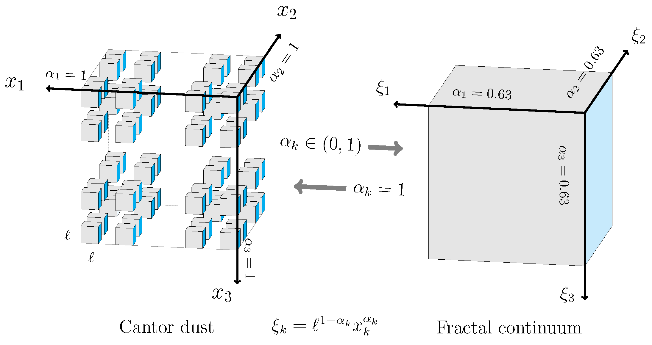
A norm fractal continuum $\Vert N\Vert ={\left[{\sum }_k^3{\xi }_k^{2\beta }\right]}^{1/2\beta }$, where $\beta =d_{ch}/3\le 1$, and the transformation of the integer coordinates $x_k\in {\Re }^3$ to the fractal coordinates ${\xi }_k\in F^{\alpha }\subset {\Re }^3$ is given by the proportionality constant

$$\begin{array}{c}\hfill {\xi }_k={\mathsf{\ell }}^{1-{\alpha }_k}{x}_k^{{\alpha }_k},\end{array}$$

(2)

where ℓ is the box size in the ith-iteration of fractal set. Integer and fractal configurations are shown in Figure 2.

ii

The distance between two points $A,B\in F^{\alpha }$ is defined as $\Delta (A,B)={\left[{\sum }_k^3{\Delta }_k^{2\beta }\right]}^{1/2\beta }$, where ${\Delta }_k=\Vert {\xi }_{ak}-{\xi }_{bk}\Vert$.

iii

The fractal continuum gradient ${\nabla }^{\alpha }={\mathbf{e}}_k{\nabla }_k^{\alpha }$, where ${\mathbf{e}}_k$ denotes basis vectors and

$$\begin{array}{c}\hfill {\nabla }_k^{\alpha }={\left(c_1^{\left(k\right)}\right)}^{-1}{\nabla }_k\end{array}$$

(3)

is the definition of the spatial fractal continuum derivative, with $c_1^{\left(k\right)}={\alpha }_k{\mathsf{\ell }}^{1-{\alpha }_k}{x}_k^{{\alpha }_k-1}$. The divergence operator is ${\nabla }^{\alpha }·\overrightarrow{F}$.

iv

Therefore, the Laplacian is expressed by [13,19] as ${\Delta }^{\alpha }={\nabla }^{\alpha }·({\nabla }^{\alpha }·\overrightarrow{F})={\sum }_k^3{\left(c_1^{\left(k\right)}\right)}^{-2}$$\left[{\nabla }_k^2+{\displaystyle \frac{\beta -{\alpha }_k}{x_k}}{\nabla }_k\right]$.

3.2. Fractal Continuum Elasticity

On the other hand, the elasticity in the fractal continuum concept is suggested in [41], where the governing equations are as follows:

(a)

The momentum conservation equation is

$$\begin{array}{c}\hfill {\nabla }_k^{{\alpha }_k}{\sigma }_{ij}+f_{bi}=0,\end{array}$$

(4)

where ${\sigma }_{ij}$ denotes the stress tensor, $f_{bi}$ represents the body forces, and ${\nabla }_j^{{\alpha }_k}={\partial }^{{\alpha }_k}/\partial x_j^{{\alpha }_k},j,k=1,2,3$.

(b)

The strain tensor is defined in fractal continuum dimensions as follows [18]:

$$\begin{array}{c}\hfill {\epsilon }_{ij}^{\alpha }=2^{-1}\left[{\nabla }_j^{\alpha }{v}_i+{\nabla }_i^{\alpha }{v}_j\right].\end{array}$$

(5)

(c)

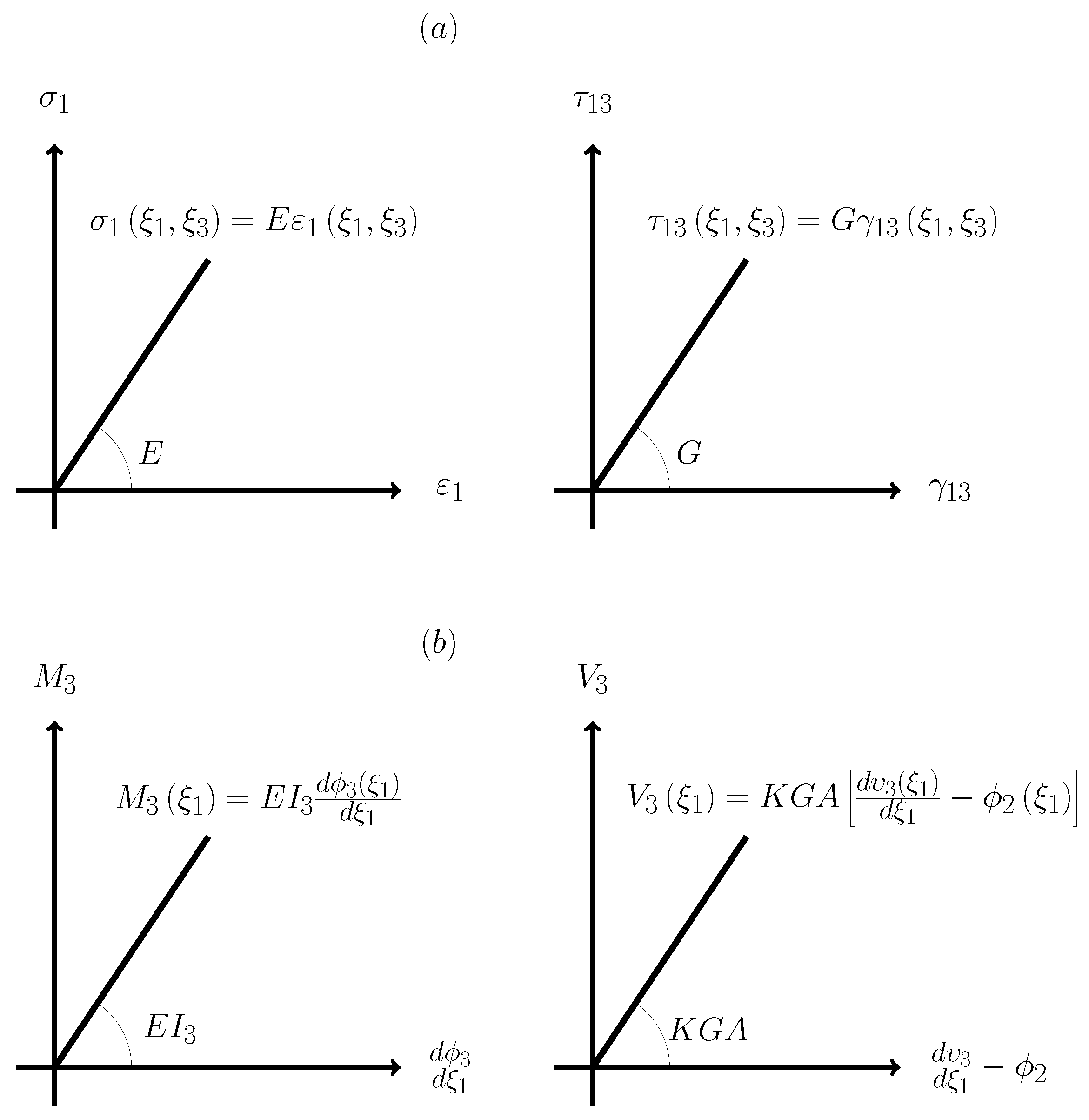
The constitutive relationship between stress and strain for a linear elastic isotropic domain is given as ${\sigma }_{ij}=\mu ({\nabla }_j^{\alpha }{v}_i+{\nabla }_i^{\alpha }{v}_j)+\lambda {\nabla }^{\alpha }{\upsilon }_k{\delta }_{ij}$, where the term in parentheses is the deformation tensor ${\epsilon }_{ij}^{\alpha }$, where $\lambda$ and $\mu$ are the Lamé parameters of the fractal continuum and the components of the fractal displacement vectors ${\upsilon }_k\in F^{\alpha }$ can be expressed in Cartesian coordinates as

$$\begin{array}{c}\hfill {\upsilon }_k={\alpha }_k{\mathsf{\ell }}^{1-{\alpha }_k}{x}_k^{{\alpha }_k-1}{u}_k.\end{array}$$

(6)

where $u_k\in F$ denotes the Euclidean components of the displacement vector.

4. Timoshenko Beam Fourth-Order Fractal Equation

In this section, the fractal single equation of the Timoshenko beam principle is suggested.

Deduction in Fractal Space

The displacement field in a fractal continuum framework is given by ${\upsilon }_1({\xi }_1,{\xi }_3)={\xi }_3\theta \left({\xi }_1\right),$${\upsilon }_2=({\xi }_1,{\xi }_3)=0,{\upsilon }_3({\xi }_1,{\xi }_3)={\upsilon }_3\left({\xi }_1\right)$, where ${\upsilon }_3$ is the cross-section fractal displacement at point $({\xi }_1,0)$, which is located in the middle of the plane, where ${\xi }_3=0$ and $\theta$ denotes the beam cross-section displacement (see Figure 3); therefore the strain displacement relationship is defined by

$$\begin{array}{c}\hfill {\epsilon }_{11}={\displaystyle \frac{\partial {\upsilon }_1}{\partial {\xi }_1}}={\xi }_3{\displaystyle \frac{d\theta }{d{\xi }_1}}\end{array}$$

(7)

and

$$\begin{array}{c}\hfill {\gamma }_{13}={\displaystyle \frac{\partial {\upsilon }_1}{\partial {\xi }_3}}+{\displaystyle \frac{\partial {\upsilon }_3}{\partial {\xi }_1}}=\theta +{\displaystyle \frac{d{\upsilon }_3}{d{\xi }_1}},\end{array}$$

(8)

We define the longitudinal bending displacement as $u\left({\xi }_1,{\xi }_3\right)=-{\xi }_3{\varphi }_2$ in the same way as Euler–Bernoulli beam theory, and the curvature radius is defined by the relationship $\rho =-d{\varphi }_2/d{\xi }_1$.

Therefore, we can apply the differential curvature beam element concept, which is defined by

$$\begin{array}{c}\hfill k=-{\displaystyle \frac{1}{\rho }},\end{array}$$

(9)

since $k=-1/\rho =-d\varphi \left(x_1\right)/d{x}_1$, which can also be written as $k=-1/\rho =-M\left(x_1\right)/EI$—so, $M\left(x_1\right)=-[d\varphi \left(x_1\right)/d{x}_1]EI$.

The total rotation is the slope ${\upsilon }_3$ due to the bending motion, which is $d{\xi }_3/d{\xi }_1$ and is numerically equal to the sum of both rotations $d{\xi }_3/d{\xi }_1={\varphi }_2+{\phi }_2$, where ${\phi }_2\equiv {\gamma }_{13}\Rightarrow d{\xi }_3/d{\xi }_1={\varphi }_2+{\gamma }_{13}$, where ${\gamma }_{13}$ is the angular strain due to shear force.

The definition of curvature is equivalent to the bending moment concept given that $k=-d{\varphi }_2/d{\xi }_1$ increases and decreases proportionally to $ds$; therefore, and according to Timoshenko’s seminal work, the bending moment $M\left(x\right)$ is defined according to Equation (9) such that $k=-1/\rho \equiv -d\theta \left({\xi }_1\right)/d{\xi }_1$ and $k=-1/\rho =-M\left({\xi }_1\right)/EI$. Then

$$\begin{array}{c}\hfill M\left({\xi }_1\right)=-EI{\displaystyle \frac{d\theta \left({\xi }_1\right)}{d{\xi }_1}},\end{array}$$

(10)

as is illustrated in Figure 4. Deriving the bending moment equation and applying the first condition of equilibrium $V\left({\xi }_1\right)=dM\left({\xi }_1\right)/d{\xi }_1$, the follow expression is obtained:

$$\begin{array}{c}\hfill V\left({\xi }_1\right)={\displaystyle \frac{d^2{\varphi }_2}{d{\xi }_1^2}}.\end{array}$$

(11)

Deriving once again the last expression and by applying the second condition of equilibrium $q_3=dV\left({\xi }_1\right)/d{\xi }_1$, the following relationship is deduced:

$$\begin{array}{c}\hfill q_3=-EI{\displaystyle \frac{d^3{\varphi }_2}{d{\xi }_1^3}}.\end{array}$$

(12)

Taking into account the definition of the displacement field ${\gamma }_{13}=d{\upsilon }_3/d{\xi }_1-\varphi$, we may substitute this expression given that $\phi$ represents the strain due to the shear effect obtaining in the following equation (see Figure 4):

$$\begin{array}{c}\hfill V\left({\xi }_1\right)=KGA\left[{\displaystyle \frac{d^2{\upsilon }_3}{d{\xi }_1}}-{\varphi }_2\right].\end{array}$$

(13)

Rearranging and matching Equations (11) and (13), it is possible to write the following:

$$\begin{array}{c}\hfill EI{\displaystyle \frac{d^2{\varphi }_2}{d{\xi }_1^2}}+KGA\left[{\displaystyle \frac{d^2{\upsilon }_3}{d{\xi }_1}}-{\varphi }_2\right]=0.\end{array}$$

(14)

From Equations (11) and (13), the equilibrium condition can be rewritten, respectively, as

$$\begin{array}{c}\hfill q_3=-EI{\displaystyle \frac{d^3{\varphi }_2}{d{\xi }_1^3}}\mathrm{and}{q}_3=KGA{\displaystyle \frac{d^2{\varphi }_2}{d{\xi }_1^2}}-{\displaystyle \frac{d\varphi }{d{\xi }_1}}{q}_3.\end{array}$$

(15)

From Equation (15), the following is obtained:

$$\begin{array}{c}\hfill {\displaystyle \frac{d^2{\upsilon }_3}{d{\xi }_1}}={\displaystyle \frac{d{\varphi }_2}{d{\xi }_1}}-{\displaystyle \frac{q_3}{KGA}}.\end{array}$$

(16)

Matching both equations in (15), we obtain

$$\begin{array}{c}\hfill EI{\displaystyle \frac{d^3{\varphi }_2}{d{\xi }_1^3}}+KGA\left[{\displaystyle \frac{d^2{\upsilon }_3}{d{\xi }_1}}-{\displaystyle \frac{d{\varphi }_2}{d{\xi }_1}}\right]=0.\end{array}$$

(17)

Two-time deriving Equation (17) leads to

$$\begin{array}{c}\hfill {\displaystyle \frac{d^4{\upsilon }_3}{d{\xi }_1^4}}=EI{\displaystyle \frac{d^3{\varphi }_2}{d{\xi }_1^3}}-{\displaystyle \frac{1}{KGA}}{\displaystyle \frac{d^2{q}_3}{d{\xi }_1^2}}.\end{array}$$

(18)

Substituting Equation (15) in Equation (18), we arrive at the following outcome:

$$\begin{array}{c}\hfill {\displaystyle \frac{d^4{\upsilon }_3}{d{\xi }_1^4}}={\displaystyle \frac{q_3}{EI}}-{\displaystyle \frac{1}{KGA}}{\displaystyle \frac{d^2{q}_3}{d{\xi }_1^2}}.\end{array}$$

(19)

This allows us to ultimately obtain the expression that defines the elastic curve function for a fractal Timoshenko beam represented as a fourth-order differential equation in fractal coordinates.

Mapping from fractal to Cartesian coordinates leads us to the final single equation for Timoshenko beam theory in the fractal continuum space, which is given by

$$\begin{array}{c}\hfill {\displaystyle \frac{d^4{\upsilon }_3}{{\xi }_1^{4{\alpha }_1}}}={\displaystyle \frac{q_3}{EI}}-{\mathsf{\ell }}^{2{\alpha }_1-2}{\displaystyle \frac{1}{KGA}}{\displaystyle \frac{d^2{q}_3}{d{x}_1^{2{\alpha }_1}}}.\end{array}$$

(20)

It is a straightforward matter to see that Equation (20) is equal to Equation (1) if ${\alpha }_1=1$.

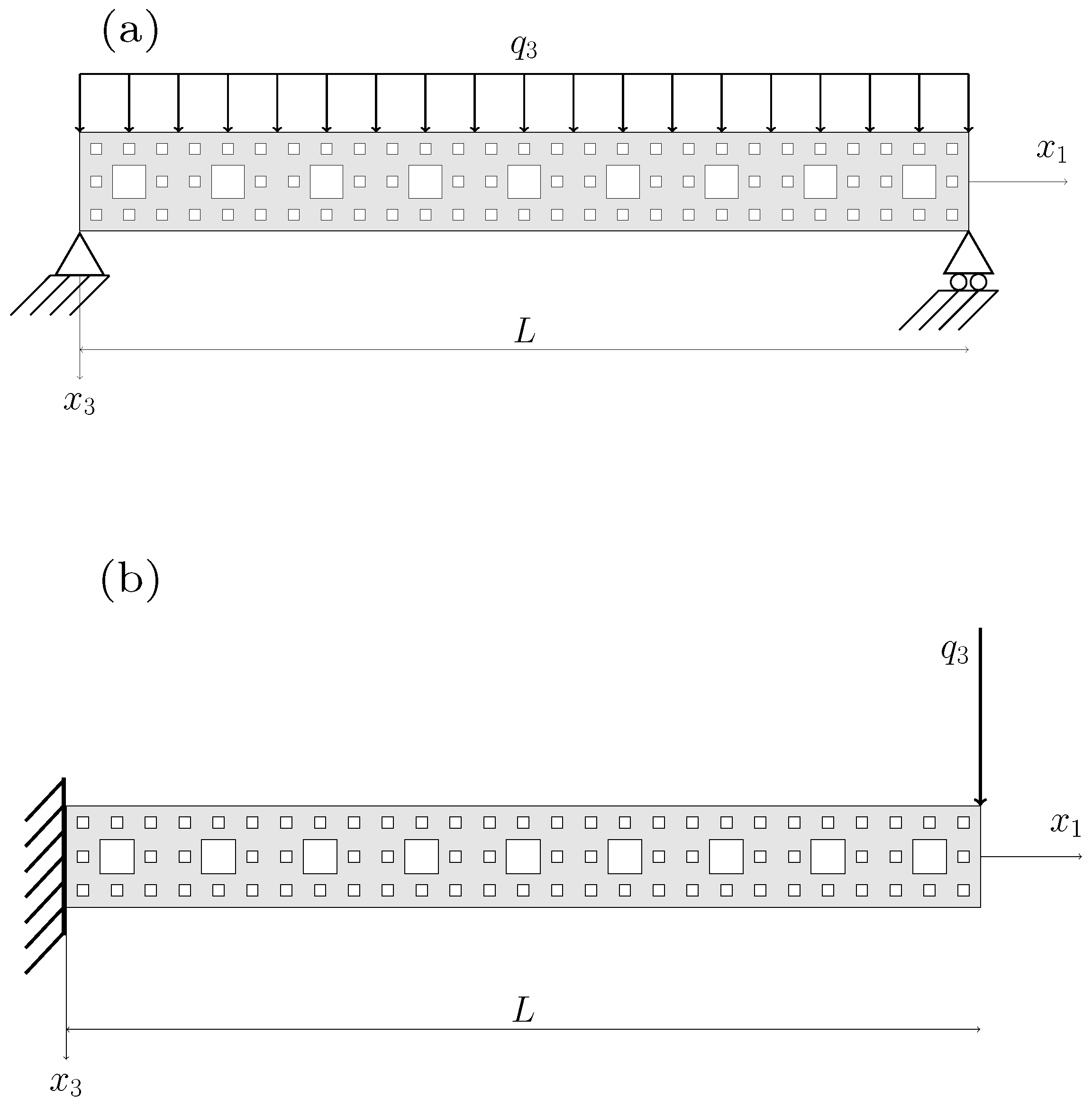
5. Bending and Rotation on Timoshenko Fractal Beams

This section is devoted to applying the Timoshenko fractal beam model on beams with classical boundary conditions.

Fractal Beams

To carry out the relevant numerical applications of the Timoshennko self-similar beam single equation, the following boundary conditions are assumed (Figure 5 shows both beams studied in this work):

1

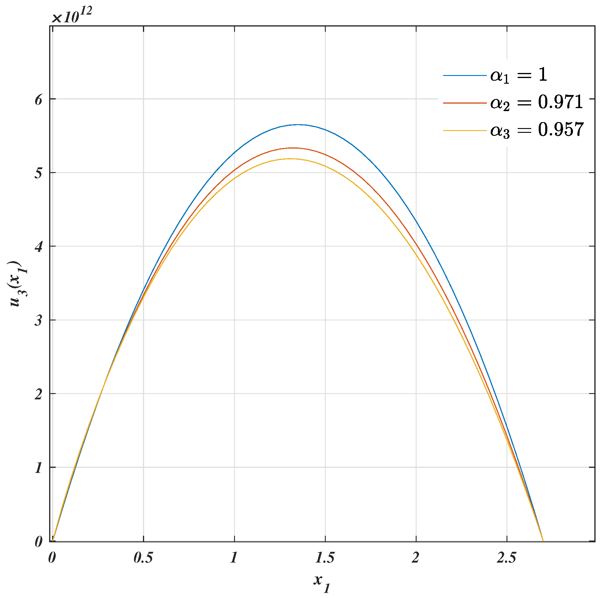
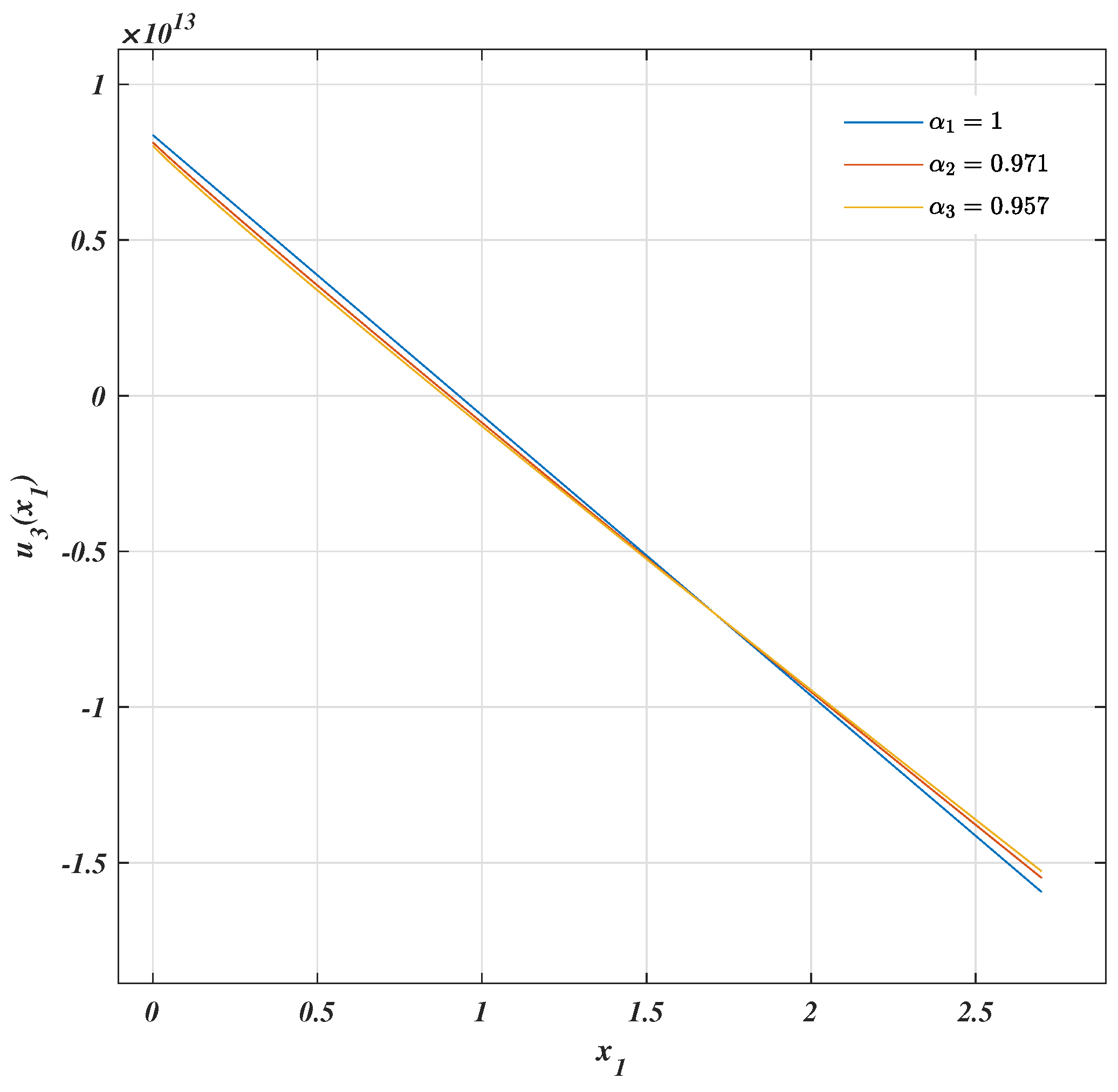
For the simply supported beam with distributed load,

$$\begin{array}{c}\hfill {\upsilon }_3\left(0\right)=M\left(0\right)={\upsilon }_3\left(L\right)=M\left(L\right)=0\end{array}$$

(21)

and then

$$\begin{array}{c}\hfill {\upsilon }_3=-{\displaystyle \frac{q{\xi }_1^4}{24EI}}-{\displaystyle \frac{qL{\xi }_1^3}{12EI}}+{\displaystyle \frac{q{L}^3{\xi }_1}{24EI}}-{\displaystyle \frac{q{\xi }_1^2}{2KGA}}+{\displaystyle \frac{qL{\xi }_1}{2KGA}}\end{array}$$

(22)

$$\begin{array}{c}\hfill {\upsilon }_3={\displaystyle \frac{q}{24EI}}\left[-{\xi }_1^4-2L{\xi }_1^3+L^3{\xi }_1\right]+{\displaystyle \frac{q}{2KGA}}\left[L{\xi }_1-{\xi }_1^2\right]\end{array}$$

(23)

2

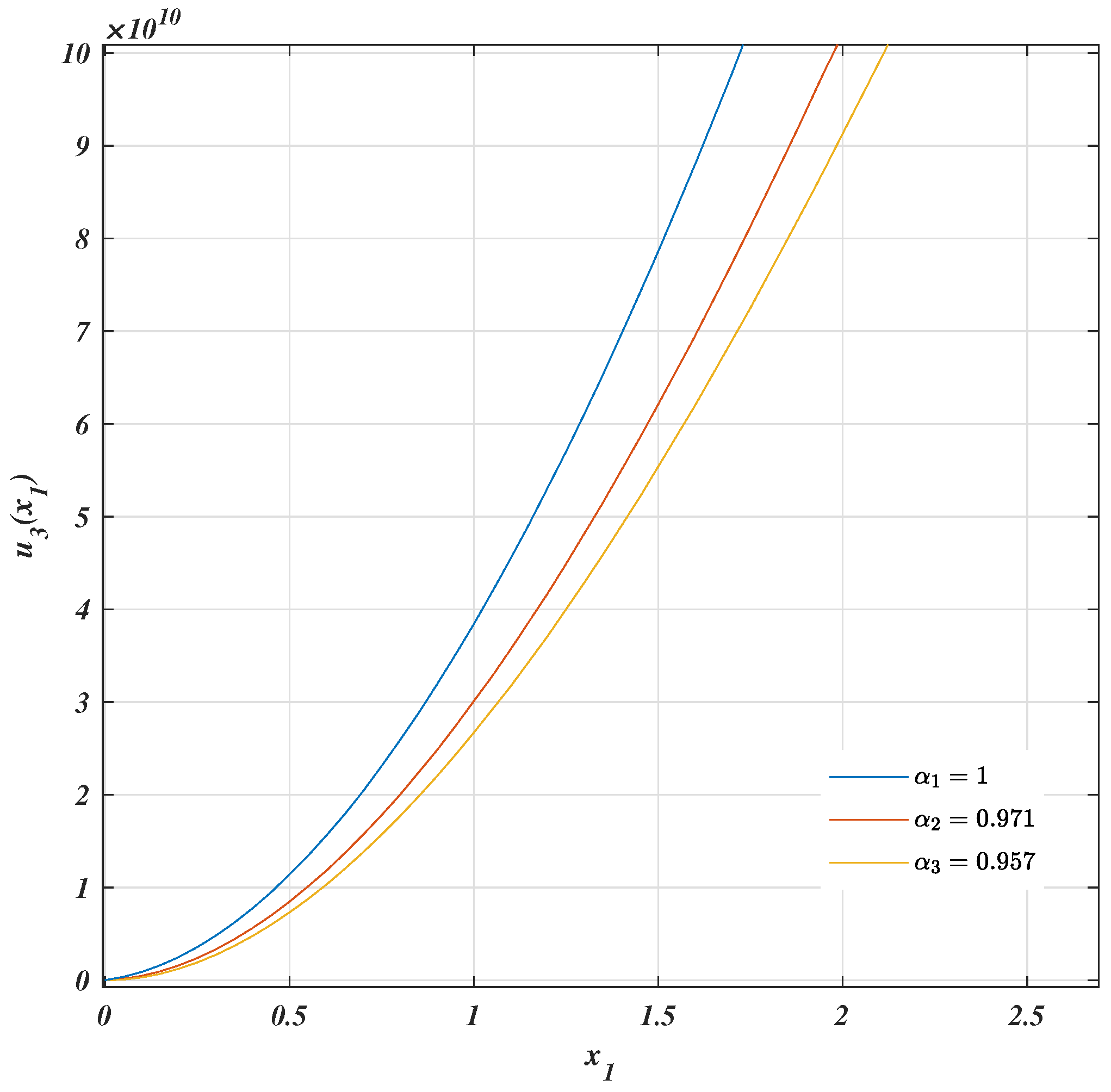
For the cantilever fractal beam with load at the free end,

$$\begin{array}{c}\hfill {\upsilon }_3\left(0\right)=\theta \left(0\right)=M\left(L\right)=V\left(L\right)=0,\end{array}$$

(24)

and therefore

$$\begin{array}{c}\hfill {\upsilon }_3=-{\displaystyle \frac{P{\xi }_1}{KGA}}+{\displaystyle \frac{P{\xi }_1{\left(2L-{\xi }_1\right)}^2}{4EI}}\end{array}$$

(25)

By transforming the above transversal displacement to Cartesian coordinates, these can be written for the simply supported beam as

$$\begin{array}{c}\hfill {\upsilon }_3=-{\displaystyle \frac{q{\mathsf{\ell }}^{4-4{\alpha }_1}{x}_1^{4{\alpha }_1}}{24EI}}-{\displaystyle \frac{q{\mathsf{\ell }}^{3-3{\alpha }_1}{L}^{{\alpha }_1}{x}_1^{3{\alpha }_1}}{12EI}}+{\displaystyle \frac{q{\mathsf{\ell }}^{1-1{\alpha }_1}{L}^{3{\alpha }_1}{x}_1^{{\alpha }_1}}{24EI}}-{\displaystyle \frac{q{{\mathsf{\ell }}^{2-2{\alpha }_1}x}_1^{2{\alpha }_1}}{2KGA}}+{\displaystyle \frac{q{\mathsf{\ell }}^{1-1{\alpha }_1}{L}^{{\alpha }_1}{x}_1^{{\alpha }_1}}{2KGA}},\end{array}$$

(26)

whereas for the cantilever beam, it is expressed by

$$\begin{array}{c}\hfill {\upsilon }_3=-{\displaystyle \frac{P{{\mathsf{\ell }}^{1-1{\alpha }_1}x}_1^{{\alpha }_1}}{KGA}}+{\displaystyle \frac{P{\mathsf{\ell }}^{1-1{\alpha }_1}{x}_1^{{\alpha }_1}{\left(2L^{{\alpha }_1}-x_1^{{\alpha }_1}\right)}^2}{4EI}},\end{array}$$

(27)

We applied the excel^R software and the fractal parameters are presented in

Table 1. Fractal parameters of beams.

Parameter	$\mathit{\eta }=0$	$\mathit{\eta }=1/9$	$\mathit{\eta }=1/5$
$d_{\mathcal{H}}$	3	2.98	2.9317
$d_{\mathcal{A}}$	2	1.99	1.9746
${\alpha }_i$	1	0.97	0.9571
ℓ	0	$2.7/3^4$	$2.7/3^4$
${\mathsf{\ell }}^{1-\alpha }{L}^{\alpha }$	2.70	2.58	2.23
$I$ ($\cdots \times {10}^{-6}$)	675	$674.897$	$673.920$

for both boundary conditions. The fractal bending and rotation for the simply supported beam are shown in Figure 6 and Figure 7, respectively. Meanwhile, the total responses for the cantilever beam are plotted in Figure 8 and Figure 9.

6. Discussion

The aim of this section is to discuss some engineering implications of the phenomenon under study based on the proposed fractal formulation.

First, the model suggested in Equation (20) matches its Euclidean version given in Equation (1) when ${\alpha }_1=1$ and validates our results for the extended fractal continuum version.

Secondly, an increment in the reduction in calculation costs and memory storage requirements is observed in the alternative fractal formulation with a single equation compared with fractional versions or with the fractal version, which have two fractal differential equations. Additionally, Equation (20), called the fourth-order Timoshenko fractal beam single equation, can be similar to the Euler–Bernoulli beam equation when the third term of Equations (1) and (20) is deleted, which is valid when $3EI/KGA{L}^2\ll 1$.

Third, from Figure 6, Figure 7, Figure 8 and Figure 9, it is easy to see the effects of fractality given by ${\alpha }_1=d_H-d_A$, which are linked with its bending stiffness $EI$ through its fractal geometry, such that when ${\alpha }_1$ approaches one the value of $EI$ is lowest.

Finally, as expected in the results, the maximum value of beam deflection is obtained when the slope is zero on the fractal beam.

The results plotted in Figure 6 and Figure 7 obtained with the single fractal equation match the fractal results published in [18], which were obtained using the two classical equations of Timoshenko beams. However, the fractal model introduced in this manuscript has the advantage that it is algorithmic and easier to plot, as sketched in the last two figures.

7. Summary

In this work, the fractal bending of Timoshenko beams based in the fractal continuum framework was studied. A new fractal approach to fractal bending of Timoshenko beams was discussed, which consists of a single equation of the fourth order similar to the Euler–Bernoulli beam equation. Also, it was shown that this Timoshenko beam reduces to Euler–Bernoulli ones when the beams analyzed are shear-rigid beams.

The variable order of the proposed fractal continuum model depends on the fractal dimension of the beam length ${\alpha }_1$, which fluctuates $0<{\alpha }_1<1$, which is linked to the Hausdorff dimension of the beam and the Hausdorff dimension of the cross-sectional area by ${\alpha }_1=d_H-d_A$. The model converges to the traditional model when $d_H=3$ and $d_A$ = 2.

This model represents an alternative solution to calculate mechanical responses in trusses, structures, and frames because it is simple, exact, and algorithmic.

References

- Falconer, K. Fractal Geometry: Mathematical Foundations and Applications; John Wiley and Sons, Ltd.: Chichester, UK, 2014. [Google Scholar]
- Damian-Adame, L.; Gutiérrez-Torres, C.; Figueroa-Espinoza, B.; Barbosa-Saldaña, J.; Jiménez-Bernal, J. A Mechanical Picture of Fractal Darcy’s Law. Fractal Fract. 2023, 7, 639. [Google Scholar] [CrossRef]
- Samayoa, D.; Damián, L.; Kriyvko, A. Map of bending problem for self-similar beams into fractal continuum using Euler-Bernoulli principle. Fractal Fract. 2022, 6, 230. [Google Scholar] [CrossRef]
- Samayoa, D.; Kriyvko, A.; Velázquez, G.; Mollinedo, H. Fractal Continuum Calculus of Functions on Euler-Bernoulli Beam. Fractal Fract. 2022, 6, 552. [Google Scholar] [CrossRef]
- Golmankhaneh-Amirreza, K.; Tunc, S.; Schlichtinger, A.M.; Asanza, D.M.; Golmankhaneh, A.K. Modeling tumor growth using fractal calculus: Insights into tumor dynamics. Biosystems 2024, 235, 105071. [Google Scholar] [CrossRef]
- Zhang, J.; Wang, Y.; Luo, X.; Luan, W.-L. Multi-Viewpoint Assessment of Urban Waterfront Skylines: Fractal and Spatial Hierarchy Analysis in Shanghai. Buildings 2025, 15, 1407. [Google Scholar] [CrossRef]
- Huang, Y.; Gong, A.; Jin, Z.; Peng, Y.; Shao, S.; Yong, K. Synergistic Effects of Alkali Activator Dosage on Carbonation Resistance and Microstructural Evolution of Recycled Concrete: Insights from Fractal Analysis and Optimal Threshold Identification. Buildings 2025, 15, 1742. [Google Scholar] [CrossRef]
- Golmankhaneh, A. Fractal Calculus and Its Applications; World Scientific: London, UK, 2022. [Google Scholar]
- Zhang, Y.; Sun, H.; Stowell, H.; Zayernouri, M.; Hansen, S. A review of applications of fractional calculus in Earth system dynamics. Chaos Solitons Fractals 2017, 102, 29–46. [Google Scholar] [CrossRef]
- Parvate, A.; Satin, S.; Gangal, A.D. Calculus on fractal curves in Rn. Fractals 2011, 19, 15–27. [Google Scholar] [CrossRef]
- Tarasov, V.E. General Fractional Vector Calculus. Phys. Lett. A 2005, 336, 167–178. [Google Scholar] [CrossRef]
- Balankin, A.S.; Elizarraraz, B.E. Hydrodynamics of fractal continuum flow. Phys. Rev. E 2012, 85, 025302(R). [Google Scholar] [CrossRef]
- Balankin, A.S.; Elizarraraz, B.E. Map of fluid flow in fractal porous medium into fractal continuum flow. Phys. Rev. E 2012, 85, 056314. [Google Scholar] [CrossRef]
- Stempin, P.; Sumelka, W. Space-fractional Euler-Bernoulli beam model—Theory and identification for silver nanobeam bending. Int. J. Mech. Sci. 2020, 186, 105902. [Google Scholar] [CrossRef]
- Lazopoulos, K.A.; Lazopoulos, A.K. On fractional bending of beams with A-fractional derivative. Arch. Appl. Mech. 2020, 90, 573–584. [Google Scholar] [CrossRef]
- Stempin, P.; Sumelka, W. Formulation and experimental validation of space-fractional Timoshenko beam model with functionally graded materials effects. Comput. Mech. 2021, 68, 697–708. [Google Scholar] [CrossRef]
- Wang, C.M.; Reddy, J.N.; Lee, K.H. Shear Deformable Beam and Plates; Elsevier: Oxford, UK, 2000. [Google Scholar]
- Samayoa, D.; Alcántara, A.; Mollinedo, H.; Barrera-Lao, F.; Torres-SanMiguel, C. Fractal Continuum Mapping Applied to Timoshenko Beams. Mathematics 2023, 11, 3492. [Google Scholar] [CrossRef]
- Balankin, A.S. A continuum framework for mechanics of fractal materials I: From fractional space to continuum with fractal metric. Eur. Phys. J. B 2015, 88, 90. [Google Scholar] [CrossRef]
- Shan, J.; Zhuang, C.; Loong, C.N. Parametric identification of Timoshenko-beam model for shear-wall structures using monitoring data. Mech. Syst. Signal Process. 2023, 189, 110100. [Google Scholar] [CrossRef]
- Ochsner, A. Classical Beam Theories of Structural Mechanics; Springer Nature: Cham, Switzerland, 2021. [Google Scholar]
- Ahmed, A.; Abdussalam, M. Euler-Bernoulli and Timoshenko Beam Theories Analytical and Numerical Comprehensive Revision. Eur. J. Eng. Technol. Res. 2021, 6, 20–32. [Google Scholar] [CrossRef]
- Li, X.F. A unified approach for analyzing static and dynamic behaviors of functionally graded Timoshenko and Euler–Bernoulli beams. J. Sound Vib. 2008, 318, 1210–1229. [Google Scholar] [CrossRef]
- Jiang, L.; Yan, Z. Timoshenko beam model for static bending of nanowires with surface effects. Phys. E Low-Dimens. Syst. Nanostruct. 2010, 42, 2274–2279. [Google Scholar] [CrossRef]
- Doeva, O.; Masjedi, P.K.; Weaver, P.M. Exact analytical solution for static deflection of Timoshenko composite beams on two-parameter elastic foundations. Thin-Walled Struct. 2022, 172, 108812. [Google Scholar] [CrossRef]
- Pirrotta, A.; Cutrona, S.; Lorenzo, S.D.; Matteo, A.D. Fractional visco-elastic Timoshenko beam deflection via single equation. Int. J. Numer. Methods Eng. 2015, 104, 869–886. [Google Scholar] [CrossRef]
- Lu, G.; Liu, X.; Cai, G.; Sun, J.; Zhu, D. Hybrid control of attitude maneuver and structural vibration for a large phased array antenna satellite. J. Frankl. Inst. 2024, 361, 398–417. [Google Scholar] [CrossRef]
- Guzman-Acevedo, G.M.; Vazquez-Becerra, G.E.; Quintana-Rodriguez, J.A.; Gaxiola-Camacho, J.R.; Anaya-Diaz, M.; Mediano-Martinez, J.C.; Viramontes, F.J.C. Structural health monitoring and risk assessment of bridges integrating InSAR and a calibrated FE model. Structures 2024, 63, 106353. [Google Scholar] [CrossRef]
- Relaño, C.; Muñoz, J.; Monje, C.A.; Martínez, S.; González, D. Modeling and Control of a Soft Robotic Arm Based on a Fractional Order Control Approach. Fractal Fract. 2023, 7, 8. [Google Scholar] [CrossRef]
- Liu, L.; Jiang, L.; Zhou, W.; Liu, X.; Feng, Y. An Analytical Solution for the Geometry of High-Speed Railway CRTS III Slab Ballastless Track. Mathematics 2022, 10, 3306. [Google Scholar] [CrossRef]
- Chen, K.; Wang, R.; Niu, Z.; Wang, P.; Sun, T. Topology design and performance optimization of six-limbs 5-DOF parallel machining robots. Mech. Mach. Theory 2023, 185, 105333. [Google Scholar] [CrossRef]
- Luo, W.; Wang, B.; Wang, W.; Li, Q.; Liu, X. Track structure influence analysis on metro bogie frame dynamic stress with a rigid-flexible coupled model. Eng. Fail. Anal. 2025, 171, 109357. [Google Scholar] [CrossRef]
- Kryvko, A.; González, E.J.B.; Samayoa, D. Failure analysis of anchorage of cable-stayed bridge with internal defects. Sci. Prog. 2021, 104, 368504211041481. [Google Scholar] [CrossRef]
- López, J.A.; Carrión, F.J.; Quintana, J.A.; Samayoa, D.; Lomelí, M.G.; Orozco, P.R. Verification of the Ultrasonic Qualification for Structural Integrity of Partially Concrete Embedded Steel Elements. In Proceedings of the XVII International Materials Research Congress, Cancún, Mexico, 18–21 August 2008; Advanced Materials Research. Trans Tech Publications Ltd.: Zurich, Switzerland, 2009; Volume 65, pp. 69–78. [Google Scholar] [CrossRef]
- Liu, Z.; Tang, Z.; Li, J.; Hu, Z.; Qin, X.; Shi, B.; Mao, S.; Qiu, Y.; Zhu, Z. Tri-cortical pedicle screw fixation in the most cranial instrumented segment to prevent proximal junctional kyphosis. Spine J. 2025, 1–10. [Google Scholar] [CrossRef]
- Carpinteri, A.; Pugno, N.; Sapora, A. Asymptotic analysis of a von Koch beam. Chaos Soliton Fractals 2009, 41, 795–802. [Google Scholar] [CrossRef]
- Loong, C.; Dimitrakopoulos, E. The static stability of evolving fractal beams as a dynamical system. Proc. R. Soc. A 2025, 481, 48120240918. [Google Scholar] [CrossRef]
- Carpinteri, A.; Pugno, N.; Sapora, A. Free vibration analysis of a von Koch beam. Int. J. Solids Struct. 2010, 47, 1555–1562. [Google Scholar] [CrossRef]
- Carpinteri, A.; Pugno, N.; Sapora, A. Dynamic response of damped von Koch antennas. J. Vib. Control 2011, 17, 733–740. [Google Scholar] [CrossRef]
- Méndez-Márquez, E.; Reyes de Luna, E.; De León, D.; Carrión-Viramontes, F.J.; Kryvko, A.; Samayoa, D. Free vibration analysis on fractal beams. Eur. J. Mech. A/Solids 2025, 114, 105719. [Google Scholar] [CrossRef]
- Balankin, A.S. Stresses and strains in a deformable fractal medium and in its fractal continuum model. Phys. Lett. A 2013, 377, 2535–2541. [Google Scholar] [CrossRef]